The Reconstruction of Non-Minimal Derivative Coupling Inflationary Potentials


1
School of Mathematics and Physics, Hubei Polytechnic University, Huangshi 435003, China
2
Department of Astronomy, Beijing Normal University, Beijing 100087, China
3
School of Physics, Huazhong University of Science and Technology, Wuhan 430074, China
*
Author to whom correspondence should be addressed.
Universe 2020, 6(11), 213; https://0-doi-org.brum.beds.ac.uk/10.3390/universe6110213
Submission received: 8 October 2020
/
Revised: 18 November 2020
/
Accepted: 18 November 2020
/
Published: 19 November 2020
(This article belongs to the Special Issue Inflation, Black Holes and Gravitational Waves)
Abstract
:We derive the reconstruction formulae for the inflation model with the non-minimal derivative coupling term. If reconstructing the potential from the tensor-to-scalar ratio r, we could obtain the potential without using the high friction limit. As an example, we reconstruct the potential from the parameterization , which is a general form of the -attractor. The reconstructed potential has the same asymptotic behavior as the T- and E-model if we choose and . We also discuss the constraints from the reheating phase by assuming the parameter of state equation during reheating is a constant. The scale of big-bang nucleosynthesis could put an upper limit on if and a low limit on if .
1. Introduction
In the standard big-bang cosmology, inflation has successfully solved various problems, such as the flatness, horizon and monopole problems. Besides, its quantum fluctuation can produce the seed of the formation of large-scale structure [1,2,3,4]. A scalar field with a flat potential is usually chosen to investigate inflation. The most economical and fundamental candidate for the inflaton is therefore the Standard Model Higgs boson. However, the Higgs boson is disfavored by the observational data [3,5] when minimally coupled to gravity due to its large tensor-to-scalar ratio. If the kinetic term of the scalar field is non-minimal coupled to Einstein tensor, the tensor-to-scalar ratio r could be reduced to being consistent with the observational data, and the effective Higgs self-coupling could be the order of 1 [6,7]. This inflation model with non-minimal derivative coupling belongs to the subclass of the Horndeski theory [8], which is a general scalar–tensor theory, with field equations that are at most of the second-order derivatives of both the metric and scalar field in four dimensions [9]. Therefore, the non-minimal derivative coupling inflation model could save the Higgs model without introducing a new degree of freedom. For more about the non-minimal derivative coupling inflation model, refer to [10,11,12,13,14,15,16,17].
The most important observables of inflation are the spectral tilt and the tensor-to-scalar ratio r. To be compared with the observational data easily, they are usually expressed by the e-folding number N before the end of inflation at the horizon exit of the pivotal scale. Among them, one of the predictions that is greatly favored by the observational data may be the -attractors, and . Numerous inflation models make the -attractors prediction, for example the Starobinsky model [1], the Higgs inflation with a non-minimal coupling in the strong coupling limit [18,19], the pole inflation with the kinetic term being [20] and the T/E model [21,22]. It is therefore worth studying whether there are still other models that can make the prediction of -attractors. In this paper, we consider the non-minimal derivative coupling inflation models to investigate this -attractors issue by reconstructing the potential. Starting from the observational data and parameterizing the observable with N, using the relationships between the observable and the potential, we can then reconstruct the potential [23,24]. By this reconstruction, the model parameters can be constrained easily and the reconstructed potential would always be consistent with the observational data [24,25,26,27,28,29,30,31,32,33,34,35,36,37,38,39,40,41,42,43,44,45,46,47].
After the inflation, it is followed by the reheating phase, which may give additional constraints on the inflation phase [46,48]. Assuming that the effective parameter of state equation during reheating is a constant and the entropy is a conserved quantity, we can relate the e-folding number and the energy scale during reheating to those during inflation [48,49,50,51,52,53,54]. From these relations, the constraints on the energy scale during reheating would transfer to the constraints on the inflation model.
In this paper, we reconstruct the inflationary potentials of the non-minimal coupling inflation models and research the additional constraints from the reheating phase. The paper is organized as follows. In Section 2, we give a brief review about the inflation model with the non-minimal derivative coupling term and the reconstruction method. In Section 3, we reconstruct the potential from the parameterization of tensor-to-scalar ratio r. We discuss the constraints from the reheating in Section 4, and give the conclusion in Section 5.
2. The Relations
In this section, we develop the formulae for the reconstruction of the inflationary potential with the kinetic term non-minimal coupled to Einstein tensor. We start from the action
where we choose the unit and the coupling parameter M is a constant with the dimension of mass. For the homogeneous and isotropic Universe with the Robertson–Walker metric
where in the inflation epoch, the action (1) becomes
The kinetic term of this model is
so there are no ghosts in this model. The scale range of the parameter M is very broad. If M is extremely larger than the Hubble parameter, , the non-minimal derivative coupling term can be neglected and the model reduces to the canonical case. If M is extremely smaller than the Hubble parameter, , the non-minimal derivative coupling term dominates the inflation, and may make some new predictions different from the canonical case.
The Friedmann equation is
where is the friction parameter. The equation of motion for the scalar field is
For the slow-roll inflation, the slow-roll conditions are
Under these slow-roll conditions, the background Equations (5) and (6) become
where . With Equation (8), the friction parameter becomes
The corresponding slow-roll parameters are
Using Equations (8), (9) and (11), we obtain
The derivative of with respect to t is [10]
By using the relation , to the first order of slow-roll parameters, Equation (14) becomes
where N is the e-folding number before the end of inflation at the horizon exit. The power spectrum for the scalar perturbation is [10]
The power spectrum for the tensor perturbation is [10]
The scalar tilt and the tensor-to-scalar ratio r are [10,55]
From Equations (15) and (18), we obtain the relation between and ,
From Equations (5) and (13), we obtain the relation between and N,
where the sign ± depends on the sign of . Without loss of generality, in this paper, we only research the ‘+’ case. Combining Equations (11) and (21), we get the relation between the potential and the slow-roll parameter,
By using Equations (10) and (19), Equations (16), (20) and (22) become
These relations (23)–(25) do not contain the friction parameter F, thus it is possible to reconstruct the potential from the tensor-to-scalar ratio without using the high friction limit. In the following sections, we discuss this issue.
3. The Reconstruction
In this section, we reconstruct the potential from the tensor-to-scalar ratio r. The observational data favor small r, and the -attractor gives , which is small enough to be consistent with the observational data when . In this section, we discuss a general parameterization of the -attractor
where , and accounts for the contribution from the scalar field at the end of the inflation. From the relation (24), we obtain the spectral tilt
With the help of relation (25), we obtain the potential
Combining the slow-roll Friedmann Equation (8) and the power spectrum in Equation (23), we relate the amplitude of the power spectrum to the potential,
Substituting the reconstructed potential (28) into relation (29) and using the parameterization (26), we obtain
Combining Equations (28) and (22), we get the slow-roll parameter
where the amplitude of the friction parameter . From the condition of the end of inflation, , we obtain the relation among , and
Under the GR limit , relation (32) reduces to ; under the high friction limit , relation (32) reduces to . From Equation (26), the tensor-to-scalar ratio r under the high friction limit is therefore smaller than that under the GR limit when and is unchanged. Substituting Equation (31) into Equation (21), we get the relation between and N,
Combining it with Equation (26), the relation becomes
To the first order of tensor-to-scalar ratio r, it becomes
and the solution is
where is the integration constant. Substituting Equation (36) into Equation (28), we get the reconstructed potential
where
Therefore, we reconstruct the potential from the parameterization (26) without using the high friction limit. Furthermore, the potential (37) and parameter (38) show that the effect of the no-minimally derivative coupling term is the rescaling of the inflaton field by a factor . For the -attractors parameterization , under the GR limit , the potential reduces to [39]
If , this potential reduces to
which is asymptotic behavior of the T-model and E-model.
4. Reheating
The inflation ends when the inflaton rolls down to the minimum of the potential; around the minimum, the inflaton field will oscillate to reheat the cold universe. Because the inflation phase is followed by the reheating phase, these two phases may constrain each other, so the reheating phase may give other constraints on the inflation phase. In this section, we research the constraint from the reheating phase on the reconstructed model under the high friction limit and the GR limit .
The relation between the pivotal scale and the present Hubble parameter is
where is the e-folding number during reheating, is the scale factor at the end of reheating, and we assume the radiation domination phase follows the reheating phase immediately and the reheating phase follows inflation phase immediately. Because the physics of the reheating is still unknown, for simplicity, we assume a constant parameter of state equation during reheating, and we get
where the relation between and the temperature is
with denoting the effective number of relativistic species at reheating phase. By using the condition of the entropy conservation, we get the relation between temperature and the present cosmic microwave background temperature ,
where denotes the effective number of relativistic species for entropy, and is the present neutrino temperature. By using the above relations, we obtain [48,49]
The relations (45) and (46) show that and depend on and logarithmically, thus we choose . At the end of inflation, we have ; from Equation (13), we obtain the relation , so we have . By using the observational value of the amplitude of the power spectrum [5], from Equation (16), we have
and Equations (45) and (46) become
By using Equations (28) and (31), under the high friction limit , we obtain the constraint from the reheating process on the model parameters,
where . Under the GR limit , the relations are
where . These two situations make almost the same constraint except the e-folding difference in and the different relations of . Therefore, the friction parameter F has little influence on the reheating phase, and we just consider the high friction limit situation in the following.
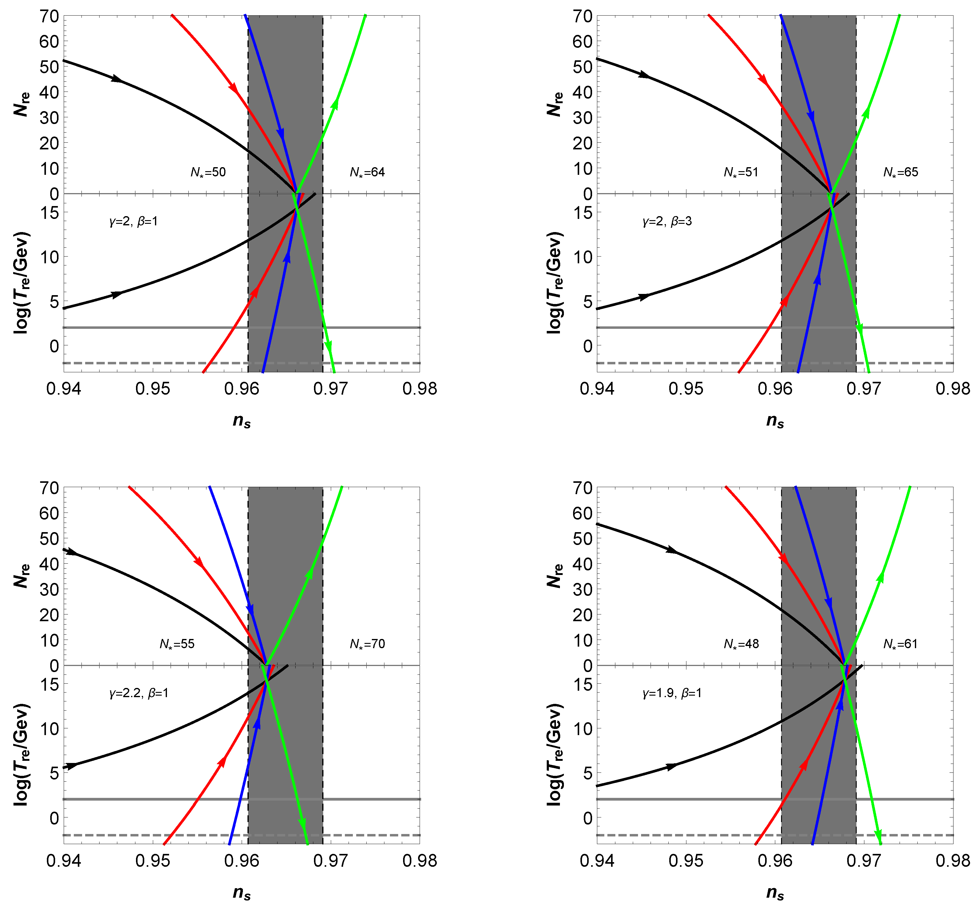
For different kinds of , , N and , by using Equations (27), (50) and (51), we calculate the corresponding spectral tilt , reheating e-folds and reheating temperature , and the results are displayed in Figure 3.
The figures show that different model parameters and and the value of provide different constraints on the reheating e-folds and the reheating temperature , while the parameter almost does not affect the reheating process. For larger spectral tilt , the allowed reheating e-folding number with , 0 and will become smaller, while the allowed reheating e-folding number with will become larger. The scale of big-bang nucleosynthesis put an upper limit on if and a low limit on if .
5. Conclusions
The non-minimal derivative coupling term in the inflation model could reduce the tensor-to-scalar ratio, which can make the large tensor-to-scalar ratio models, such as the Higgs inflation, be consistent with the observations. We derive the reconstruction formulae of the inflation model with non-minimal derivative coupling. To reconstruct the potential without using the high friction limit, we consider the parameterization of the tensor to scalar ratio inspired from the -attractor. For , which is the attractor, we get the same potential as obtained in [39], in the GR limit . When , this potential has the same asymptotic behavior as that of T/E-model. For , the potential is the exponential form. The observational constraints on the parameters are and . The reconstruction also show that the observational data favor the attractor case with .
The constraints on the spectral tilt from the Planck data could provide constraints on the reheating process. Different model parameters provide different constraints on reheating e-folds , reheating temperature and reheating state equation . For larger spectral tilt , the allowed reheating e-folding number with , 0 and will become smaller, while the allowed reheating e-folding number with will become larger. The energy scale of the reheating could also provide additional constraints on the inflation. If , and , the big bang nucleosynthesis scale requires ; if , and , the big bang nucleosynthesis scale requires .
Author Contributions
Conceptualization, Z.Y.; investigation, Q.F.; data curation, Q.F.; writing—original draft preparation, Z.Y. and Y.Y.; and writing—review and editing, Z.Y. All authors have read and agreed to the published version of the manuscript.
Funding
This research was supported in part by the National Natural Science Foundation of China under Grant No. 11947138, the Postdoctoral Science Foundation of China under Grant No. 2019M660514, the Hubei College Students’ innovation and entrepreneurship training program under Grant No. S201910920050 and the Talent-Introduction Program of Hubei Polytechnic University under Grant No.19xjk25R.
Acknowledgments
The authors thank Yungui Gong from Huazhong University of Science and Technology.
Conflicts of Interest
The authors declare no conflict of interest.
References
- Starobinsky, A.A. A New Type of Isotropic Cosmological Models Without Singularity. Phys. Lett. 1980, 91B, 99–102. [Google Scholar] [CrossRef]
- Guth, A.H. The Inflationary Universe: A Possible Solution to the Horizon and Flatness Problems. Phys. Rev. D 1981, 23, 347–356. [Google Scholar] [CrossRef] [Green Version]
- Linde, A.D. Chaotic Inflation. Phys. Lett. 1983, 129B, 177–181. [Google Scholar] [CrossRef]
- Albrecht, A.; Steinhardt, P.J. Cosmology for Grand Unified Theories with Radiatively Induced Symmetry Breaking. Phys. Rev. Lett. 1982, 48, 1220–1223. [Google Scholar] [CrossRef]
- Akrami, Y.; Arroja, F.; Ashdown, M.; Aumont, J.; Baccigalupi, C.; Ballardini, M.; Banday, A.J.; Barreiro, R.B.; Bartolo, N.; Basak, S.; et al. Planck 2018 results. X. Constraints on inflation. Astron. Astrophys. 2020, 641, A10. [Google Scholar] [CrossRef] [Green Version]
- Germani, C.; Kehagias, A. New Model of Inflation with Non-minimal Derivative Coupling of Standard Model Higgs Boson to Gravity. Phys. Rev. Lett. 2010, 105, 11302. [Google Scholar] [CrossRef] [Green Version]
- Germani, C.; Watanabe, Y.; Wintergerst, N. Self-unitarization of New Higgs Inflation and compatibility with Planck and BICEP2 data. J. Cosmol. Astropart. Phys. 2014, 1412, 9. [Google Scholar] [CrossRef] [Green Version]
- Horndeski, G.W. Second-order scalar-tensor field equations in a four-dimensional space. Int. J. Theor. Phys. 1974, 10, 363–384. [Google Scholar] [CrossRef]
- Sushkov, S.V. Exact cosmological solutions with nonminimal derivative coupling. Phys. Rev. D 2009, 80, 103505. [Google Scholar] [CrossRef] [Green Version]
- Yang, N.; Fei, Q.; Gao, Q.; Gong, Y. Inflationary models with non-minimally derivative coupling. Class. Quant. Grav. 2016, 33, 205001. [Google Scholar] [CrossRef] [Green Version]
- Yang, N.; Gao, Q.; Gong, Y. Inflation with non-minimally derivative coupling. Int. J. Mod. Phys. 2015, A30, 1545004. [Google Scholar] [CrossRef]
- Huang, Y.; Gong, Y.; Liang, D.; Yi, Z. Thermodynamics of scalar–tensor theory with non-minimally derivative coupling. Eur. Phys. J. C 2015, 75, 351. [Google Scholar] [CrossRef]
- Gong, Y.; Papantonopoulos, E.; Yi, Z. Constraints on scalar–tensor theory of gravity by the recent observational results on gravitational waves. Eur. Phys. J. C 2018, 78, 738. [Google Scholar] [CrossRef]
- Fu, C.; Wu, P.; Yu, H. Primordial Black Holes from Inflation with Nonminimal Derivative Coupling. Phys. Rev. D 2019, 100, 63532. [Google Scholar] [CrossRef] [Green Version]
- Oikonomou, V.; Fronimos, F. Reviving Non-Minimal Horndeski-Like Theories after GW170817: Kinetic Coupling Corrected Einstein-Gauss-Bonnet Inflation. arXiv 2020, arXiv:gr-qc/2006.05512. [Google Scholar]
- Odintsov, S.; Oikonomou, V.; Fronimos, F. Rectifying Einstein-Gauss-Bonnet Inflation in View of GW170817. Nucl. Phys. B 2020, 958, 115135. [Google Scholar] [CrossRef]
- Gialamas, I.D.; Karam, A.; Lykkas, A.; Pappas, T.D. Palatini-Higgs inflation with nonminimal derivative coupling. Phys. Rev. D 2020, 102, 063522. [Google Scholar] [CrossRef]
- Kaiser, D.I. Primordial spectral indices from generalized Einstein theories. Phys. Rev. D 1995, 52, 4295–4306. [Google Scholar] [CrossRef] [Green Version]
- Bezrukov, F.L.; Shaposhnikov, M. The Standard Model Higgs boson as the inflaton. Phys. Lett. B 2008, 659, 703–706. [Google Scholar] [CrossRef] [Green Version]
- Kallosh, R.; Linde, A.; Roest, D. Superconformal Inflationary α-Attractors. JHEP 2013, 11, 198. [Google Scholar] [CrossRef] [Green Version]
- Kallosh, R.; Linde, A. Universality Class in Conformal Inflation. J. Cosmol. Astropart. Phys. 2013, 1307, 2. [Google Scholar] [CrossRef] [Green Version]
- Kallosh, R.; Linde, A. Non-minimal Inflationary Attractors. J. Cosmol. Astropart. Phys. 2013, 1310, 33. [Google Scholar] [CrossRef] [Green Version]
- Huang, Q.G. Constraints on the spectral index for the inflation models in string landscape. Phys. Rev. D 2007, 76, 61303. [Google Scholar] [CrossRef] [Green Version]
- Gobbetti, R.; Pajer, E.; Roest, D. On the Three Primordial Numbers. J. Cosmol. Astropart. Phys. 2015, 1509, 58. [Google Scholar] [CrossRef] [Green Version]
- Mukhanov, V. Quantum Cosmological Perturbations: Predictions and Observations. Eur. Phys. J. C 2013, 73, 2486. [Google Scholar] [CrossRef] [Green Version]
- Roest, D. Universality classes of inflation. J. Cosmol. Astropart. Phys. 2014, 1401, 7. [Google Scholar] [CrossRef] [Green Version]
- Garcia-Bellido, J.; Roest, D. Large-N running of the spectral index of inflation. Phys. Rev. D 2014, 89, 103527. [Google Scholar] [CrossRef] [Green Version]
- Garcia-Bellido, J.; Roest, D.; Scalisi, M.; Zavala, I. Lyth bound of inflation with a tilt. Phys. Rev. D 2014, 90, 123539. [Google Scholar] [CrossRef] [Green Version]
- Garcia-Bellido, J.; Roest, D.; Scalisi, M.; Zavala, I. Can CMB data constrain the inflationary field range? J. Cosmol. Astropart. Phys. 2014, 1409, 6. [Google Scholar] [CrossRef] [Green Version]
- Creminelli, P.; Dubovsky, S.; López Nacir, D.; Simonović, M.; Trevisan, G.; Villadoro, G.; Zaldarriaga, M. Implications of the scalar tilt for the tensor-to-scalar ratio. Phys. Rev. D 2015, 2, 123528. [Google Scholar] [CrossRef] [Green Version]
- Boubekeur, L.; Giusarma, E.; Mena, O.; Ramírez, H. Phenomenological approaches of inflation and their equivalence. Phys. Rev. D 2015, 91, 83006. [Google Scholar] [CrossRef] [Green Version]
- Barranco, L.; Boubekeur, L.; Mena, O. A model-independent fit to Planck and BICEP2 data. Phys. Rev. D 2014, 90, 63007. [Google Scholar] [CrossRef] [Green Version]
- Galante, M.; Kallosh, R.; Linde, A.; Roest, D. Unity of Cosmological Inflation Attractors. Phys. Rev. Lett. 2015, 114, 141302. [Google Scholar] [CrossRef] [PubMed] [Green Version]
- Chiba, T. Reconstructing the inflaton potential from the spectral index. PTEP 2015, 2015, 73E02. [Google Scholar] [CrossRef] [Green Version]
- Cicciarella, F.; Pieroni, M. Universality for quintessence. J. Cosmol. Astropart. Phys. 2017, 1708, 10. [Google Scholar] [CrossRef] [Green Version]
- Lin, J.; Gao, Q.; Gong, Y. The reconstruction of inflationary potentials. Mon. Not. R. Astron. Soc. 2016, 459, 4029–4037. [Google Scholar] [CrossRef]
- Nojiri, S.; Odintsov, S.D. Unified cosmic history in modified gravity: From F(R) theory to Lorentz non-invariant models. Phys. Rept. 2011, 505, 59–144. [Google Scholar] [CrossRef] [Green Version]
- Odintsov, S.D.; Oikonomou, V.K. Inflationary α-attractors from F(R) gravity. Phys. Rev. D 2016, 94, 124026. [Google Scholar] [CrossRef] [Green Version]
- Yi, Z.; Gong, Y. Nonminimal coupling and inflationary attractors. Phys. Rev. D 2016, 94, 103527. [Google Scholar] [CrossRef] [Green Version]
- Odintsov, S.D.; Oikonomou, V.K. Inflation with a Smooth Constant-Roll to Constant-Roll Era Transition. Phys. Rev. D 2017, 96, 24029. [Google Scholar] [CrossRef] [Green Version]
- Nojiri, S.; Odintsov, S.D.; Oikonomou, V.K. Constant-roll Inflation in F(R) Gravity. Class. Quant. Grav. 2017, 34, 245012. [Google Scholar] [CrossRef] [Green Version]
- Choudhury, S. COSMOS-e′-soft Higgsotic attractors. Eur. Phys. J. C 2017, 77, 469. [Google Scholar] [CrossRef] [Green Version]
- Gao, Q.; Gong, Y. Reconstruction of extended inflationary potentials for attractors. Eur. Phys. J. Plus 2018, 133, 491. [Google Scholar] [CrossRef]
- Jinno, R.; Kaneta, K. Hill-climbing inflation. Phys. Rev. D 2017, 96, 43518. [Google Scholar] [CrossRef] [Green Version]
- Gao, Q. Reconstruction of constant slow-roll inflation. Sci. China Phys. Mech. Astron. 2017, 60, 90411. [Google Scholar] [CrossRef] [Green Version]
- Fei, Q.; Gong, Y.; Lin, J.; Yi, Z. The reconstruction of tachyon inflationary potentials. J. Cosmol. Astropart. Phys. 2017, 1708, 18. [Google Scholar] [CrossRef] [Green Version]
- Koh, S.; Lee, B.H.; Tumurtushaa, G. Reconstruction of the Scalar Field Potential in Inflationary Models with a Gauss-Bonnet term. Phys. Rev. D 2017, 95, 123509. [Google Scholar] [CrossRef] [Green Version]
- Dai, L.; Kamionkowski, M.; Wang, J. Reheating constraints to inflationary models. Phys. Rev. Lett. 2014, 113, 41302. [Google Scholar] [CrossRef] [Green Version]
- Cook, J.L.; Dimastrogiovanni, E.; Easson, D.A.; Krauss, L.M. Reheating predictions in single field inflation. J. Cosmol. Astropart. Phys. 2015, 1504, 47. [Google Scholar] [CrossRef]
- Ueno, Y.; Yamamoto, K. Constraints on α-attractor inflation and reheating. Phys. Rev. D 2016, 93, 83524. [Google Scholar] [CrossRef] [Green Version]
- Kabir, R.; Mukherjee, A.; Lohiya, D. Reheating Constraints on Kähler Moduli Inflation. arXiv 2016, arXiv:gr-qc/1609.09243. [Google Scholar] [CrossRef] [Green Version]
- Di Marco, A.; Cabella, P.; Vittorio, N. Reconstruction of α-attractor supergravity models of inflation. Phys. Rev. D 2017, 95, 23516. [Google Scholar] [CrossRef]
- Dimopoulos, K.; Owen, C. Quintessential Inflation with α-attractors. J. Cosmol. Astropart. Phys. 2017, 1706, 27. [Google Scholar] [CrossRef] [Green Version]
- Gong, J.O.; Pi, S.; Leung, G. Probing reheating with primordial spectrum. J. Cosmol. Astropart. Phys. 2015, 5, 27. [Google Scholar] [CrossRef] [Green Version]
- Tsujikawa, S. Observational tests of inflation with a field derivative coupling to gravity. Phys. Rev. D 2012, 85, 83518. [Google Scholar] [CrossRef] [Green Version]
Figure 1.
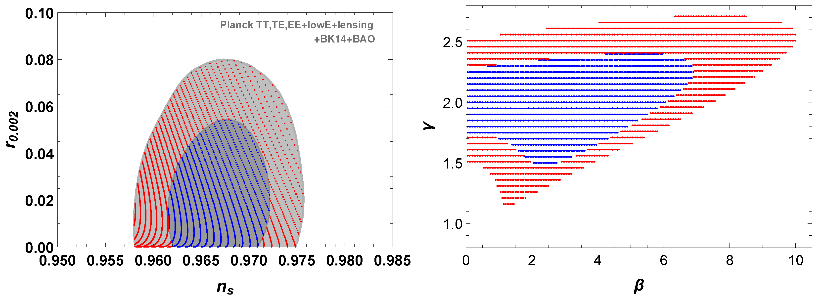
The constraints on and from Planck data [5] and the theoretical predictions for the parameterization (26) in the high friction limit. The Planck constraints on and r are displayed in the left panel and the constraints on and for are displayed in the right panel. The red and blue regions denote the and confidence level, respectively.
Figure 1.
The constraints on and from Planck data [5] and the theoretical predictions for the parameterization (26) in the high friction limit. The Planck constraints on and r are displayed in the left panel and the constraints on and for are displayed in the right panel. The red and blue regions denote the and confidence level, respectively.

Figure 2.
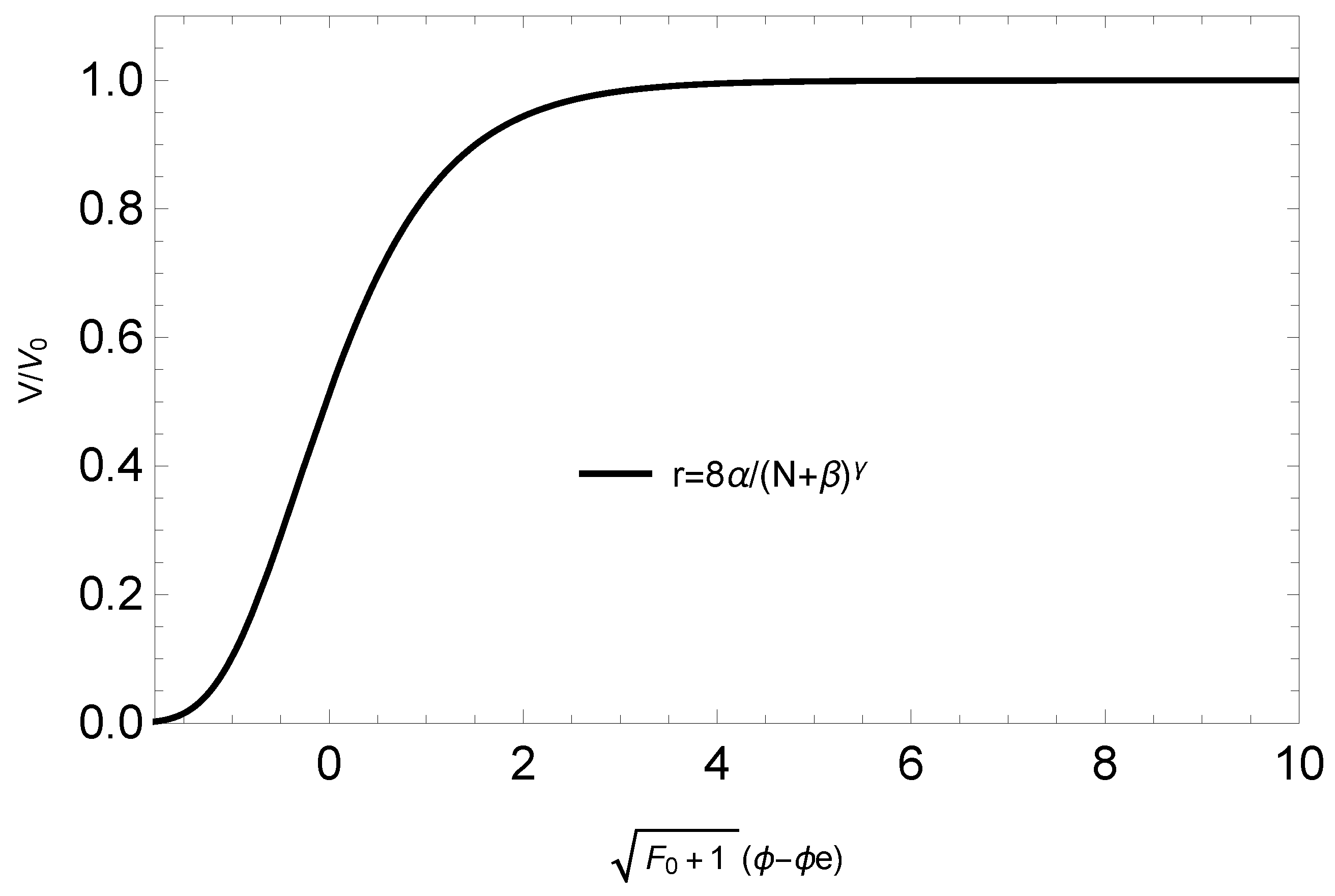
The reconstructed potentials are normalized with from Equation (30), and the inflaton field is normalized with . We choose the value of that could make .
Figure 2.
The reconstructed potentials are normalized with from Equation (30), and the inflaton field is normalized with . We choose the value of that could make .

Figure 3.
(Top) The relations between and ; and (Bottom) the relations between and . The corresponding values of and for each model are indicated in each panel. The Planck constraint [5] is denoted by the gray band, and the Planck constraint on the e-folds N is also indicated. The black, red, blue and green lines correspond to the reheating models with , 0, 1/6 and 2/3, respectively; in each line, the arrow denotes the direction of N enlargement. The horizontal gray solid and dashed lines in the bottom panels denote the electroweak scale GeV and the big bang nucleosynthesis scale MeV, respectively.

Publisher’s Note: MDPI stays neutral with regard to jurisdictional claims in published maps and institutional affiliations. |
© 2020 by the authors. Licensee MDPI, Basel, Switzerland. This article is an open access article distributed under the terms and conditions of the Creative Commons Attribution (CC BY) license (http://creativecommons.org/licenses/by/4.0/).
Share and Cite
MDPI and ACS Style
Fei, Q.; Yi, Z.; Yang, Y. The Reconstruction of Non-Minimal Derivative Coupling Inflationary Potentials. Universe 2020, 6, 213. https://0-doi-org.brum.beds.ac.uk/10.3390/universe6110213
AMA Style
Fei Q, Yi Z, Yang Y. The Reconstruction of Non-Minimal Derivative Coupling Inflationary Potentials. Universe. 2020; 6(11):213. https://0-doi-org.brum.beds.ac.uk/10.3390/universe6110213
Chicago/Turabian StyleFei, Qin, Zhu Yi, and Yingjie Yang. 2020. "The Reconstruction of Non-Minimal Derivative Coupling Inflationary Potentials" Universe 6, no. 11: 213. https://0-doi-org.brum.beds.ac.uk/10.3390/universe6110213
Note that from the first issue of 2016, this journal uses article numbers instead of page numbers. See further details here.