Article

Correlations between Earthquake Properties and Characteristics of Possible ULF Geomagnetic Precursor over Multiple Earthquakes

by
Khairul Adib Yusof
1,2,
Mardina Abdullah
1,3,
Nurul Shazana Abdul Hamid
1,4,*,
Suaidi Ahadi
5 and
Akimasa Yoshikawa
6
1
Space Science Center, Institute of Climate Change, Universiti Kebangsaan Malaysia, Bangi 43600, Malaysia
2
Department of Physics, Faculty of Science, Universiti Putra Malaysia, Seri Kembangan 43400, Malaysia
3
Department of Electrical, Electronic and Systems Engineering, Faculty of Engineering and Built Environment, Universiti Kebangsaan Malaysia, Bangi 43600, Malaysia
4
Department of Applied Physics, Faculty of Science and Technology, Universiti Kebangsaan Malaysia, Bangi 43600, Malaysia
5
Department of Geophysics, Indonesian Agency for Meteorology, Climatology and Geophysics, Jakarta 10610, Indonesia
6
International Center for Space Weather Science and Education, Kyushu University, Fukuoka 812-8581, Japan
*
Author to whom correspondence should be addressed.
Submission received: 1 December 2020 / Revised: 7 January 2021 / Accepted: 15 January 2021 / Published: 19 January 2021
(This article belongs to the Special Issue Space Weather)

Abstract

:
In this study, we improved and adapted existing signal processing methods on vast geomagnetic field data to investigate the correlations between various earthquake properties and characteristics of possible geomagnetic precursors. The data from 10 magnetometer stations were utilized to detect precursory ultra-low frequency emission and estimate the source direction for 34 earthquakes occurring between the year 2007–2016 in Southeast Asia, East Asia, and South America regions. As a result, possible precursors of 20 earthquakes were identified (58.82% detection rate). Weak correlations were obtained when all precursors were considered. However, statistically significant and strong linear correlations ( r     0.60 ,   p   <   0.05 ) were found when the precursors from two closely located stations in Japan (Onagawa (ONW) and Tohno (TNO)) were exclusively investigated. For these stations, it was found that the lead time of the precursor is strongly (or very strongly) correlated with the earthquake magnitude, the local seismicity index, and the hypocentral depth. In addition, the error percentage of the estimated direction showed a strong correlation with the hypocentral depth. It is concluded that, when the study area is restricted to a specific location, the earthquake properties are more likely to have correlations with several characteristics of the possible precursors.

1. Introduction

A useful earthquake prediction must comprise three elements: (i) precursor detection, (ii) estimation of epicenter location, and (iii) determination of earthquake properties (e.g., hypocentral depth, epicentral distance, and magnitude). Researchers have demonstrated various non-seismic approaches to detect any kind of possible precursory proxy appearing before earthquakes. One of the most popular approaches is by studying anomalous low-frequency seismo-electromagnetic (seismo-EM) phenomena, i.e., direct lithospheric [1,2], seismo-ionospheric and seismo-atmospheric emissions [3]. In these phenomena, pre-earthquake seismo-EM emission is assumed to either directly or indirectly originate from the epicenter and is generated by one of these suggested mechanisms: (i) microfracture electrification [4], (ii) electrokinetic effect [5], (iii) electric current induction due to conductivity variation [6], and (iv) piezomagnetic effect [7].
However, the emission generally has very low intensity (~1 nT) relative to the ionospheric- or magnetospheric-originating emissions [8]. An ultra-low frequency (ULF; 0.01–0.10 Hz) emission is only slightly attenuated due to the low-pass filter function of the lithosphere [9], therefore it has the ability to propagate through the lithospheric crust to be eventually detected by ground magnetometers. Besides, the ULF range is well outside frequency ranges associated with other local disturbances, e.g., lightning discharges (extremely low frequency (ELF) radiation; 3 Hz–3 kHz) [10,11], and high-frequency (HF) ionospheric heating (ELF/very low frequency (VLF) radiation; 0.2–6.6 kHz) [12,13], hence the ULF range is unaffected by these phenomena. Thus, the observation of ULF emission holds promising potential in earthquake prediction study. Note that the definition of ULF range used in this study is widely accepted by similar studies [1,2,3,4], which is different from the International Telecommunication Union (ITU) designation, i.e., 300–3000 Hz. Moreover, seismo-EM emission is difficult to be distinguished from the much greater background natural EM field. The polarization ratio analysis (PRA) method was used in many studies where the ratio of vertical (Z) to total horizontal (G) geomagnetic field components is used as a potential precursory parameter, referred to as P Z / G parameter, e.g., [14,15]. The premise of the method is that the seismo-EM emission is assumed to be prevalent in the Z component in contrast to the magnetospheric-originating signal which dominates the G component [16]. In theory, the amplitude of P Z / G would increase anomalously due to the direct lithospheric emission a few weeks to several days before an earthquake. This observation was reported by prior studies [14,15,16].
At the same time, a few studies have questioned the validity of the PRA method as well as the claimed association between ULF anomalies and succeeding earthquakes [17,18]. In these studies, it is asserted that the close correspondence between the precursory parameter with global geomagnetic indices (e.g., Kp ) during certain periods disproves the association, while maintaining that any anomalies detected during other periods were caused by solar-terrestrial interaction. However, if there are no significant solar or magnetic events during the appearance of anomalies, then the assertions can be argued, thus, making the seismogenic origin of the anomalies plausible. Additionally, G component was found to have only moderate correlations with geomagnetic indices (e.g., Dst, Kp, ap), while the ratio of Z/G components exhibits even weaker correlations with the indices [19]. The finding may corroborate the role of the PRA method in effectively eliminating global geomagnetic influences from the precursory parameter.
The capability of the polarization ellipse (PE) method in estimating the direction of ULF/ELF seismo-atmospheric emission source have been shown by prior studies [3,20]. In these studies, the signals filtered in the ELF range ( 3 Hz) were found to be effective for this purpose. Since the highest sampling frequency f s of geomagnetic data available for the present study was 1 Hz, the highest decomposable frequency component would be f s / 2 = 0.5 Hz, which falls in the ULF range. Therefore, the effectiveness of this frequency range for direction estimation was investigated in this study. Meanwhile, the determination of the upcoming earthquake properties can be attained by studying the correlations between the precursor characteristics and the earthquake properties. Prior studies have found several possible correlations between amplitude–epicentral distance [21], lead time–magnitude and lead time–hypocentral depth [22]. Schekotov et al. [3] recently showed a linear dependence of maximum ULF depression on the local seismicity index ( K LS , see Equation (1)).
The present study elaborates the correlations between various characteristics of possible precursors (i.e., amplitude, frequency, lead time and error percentage of estimated direction) and properties of the earthquake that followed (i.e., magnitude, hypocentral depth, epicentral distance, and local seismicity index). Vast geomagnetic field data were processed using the PRA method to detect ULF precursors, and the PE method for direction estimation. The PRA method’s effectiveness was improved by introducing a new normalization process, which was then validated through a statistical analysis. A total of 34 earthquakes in Southeast Asia, East Asia and South America occurring between the years 2007–2016 were included in this study.

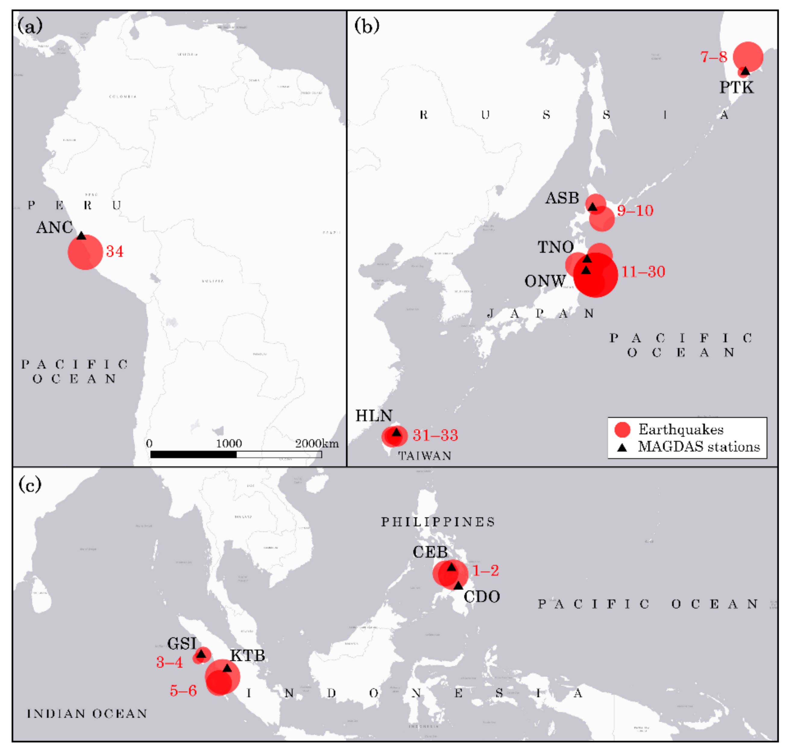
2. Instrumentation and Data Acquisition

The geomagnetic field data were acquired from the Magnetic Data Acquisition System (MAGDAS) magnetometer network through the International Center for Space Weather Science and Education (ICSWSE), Kyushu University website (http://magdas2.serc.kyushu-u.ac.jp/datausage/index.html). The network comprises a wide array of ring-core fluxgate type magnetometers located around the world [23]. The magnetometers measure parallel to three magnetic components, namely magnetic northward (H), magnetic eastward (D) and downward vertical (Z) [24]. Data from 10 MAGDAS stations (each given a code name) located in Southeast Asia, East Asia and South America were utilized in this study and their details are listed in Table 1.
A total of 34 M     5.0 earthquakes that occurred between the years 2007–2016 where the epicenters appeared within the range of 180 km from the nearest MAGDAS station were included in this study (data source: www.emsc-csem.org). The minimum magnitude, M and maximum epicentral distance, d (i.e., the distance between the epicenter and the observatory station) were selected based on the empirical threshold of 0.025 d     M 4.5 [25]. The threshold estimates that an earthquake of a magnitude as low as 4.5 potentially generates detectable ULF emission. Hence, M     5.0 was a reasonable choice since lower magnitude earthquakes occur much more frequently (Gutenberg-Richter law) and typically in swarms that complicate spatial and temporal separation of possible impacts by individual earthquakes. The empirical threshold also predicts that ULF emission generated by an M9.0 (the greatest magnitude in our study) earthquake located 180 km away is detectable. It was decided to use such a distance for all studied earthquakes to maximize the study scope.
In cases where the earthquakes occurred in a sequence, only the mainshock was included. Fundamental earthquake properties such as magnitude, M, hypocentral depth, h, epicentral distance, d, and azimuthal angle of the earthquake epicenter, ϑ EQ (i.e., the angle measured clockwise from the true North at the corresponding station) are listed in Table 2. Additionally, the local seismicity index, K LS [26] was calculated for each earthquake to quantitatively indicate seismicity condition at the station using the following equation:
K LS   =   10 0.75 M d   +   100
The location of the MAGDAS stations and earthquakes utilized in this study are illustrated in maps in Figure 1. In the maps, the earthquakes are represented as red circles and labeled with numbers, corresponding to the ID numbers as assigned in Table 2. The unbalanced distribution of studied earthquakes across the three regions was due to different frequencies of earthquake occurrence, as well as different magnetometer station densities and data availabilities located near earthquakes.
In order to distinguish possible earthquake precursors from other external sources of variation in the geomagnetic field, ap and Dst geomagnetic indices (unit: nT; sampling period: 1 h) were observed (data source: www.omniweb.gsfc.nasa.gov). Since ap and Dst are recorded by several geomagnetic observatories in mid-latitude/sub-auroral and dip-equatorial respectively [27], they were relevant for our regions of interest. Geomagnetic indices generally represent the global geomagnetic activity level which is affected by solar-terrestrial interaction. Values of ap   >   27 nT (equals Kp > 4) indicate planetary geomagnetic disturbances [28]; meanwhile, Dst   <   30 nT indicates the occurrence of at least weak geomagnetic storms [29]. Therefore, anomalies appearing during these hours must be discarded as they are likely to be due to the global geomagnetic condition [30,31]. That being said, it should be stressed that the geomagnetic indices are moderately correlated only with the G component of the raw geomagnetic field [19]. In contrast, the correlation of the indices with the precursory parameter in this study (i.e., P Z / G ) is greatly diminished due to the processing sequence in the PRA method (refer Section 3.1). Therefore, discarding the anomalies during disturbed periods can be considered as an additional precautionary measure to avoid false precursors.

3. Methodology

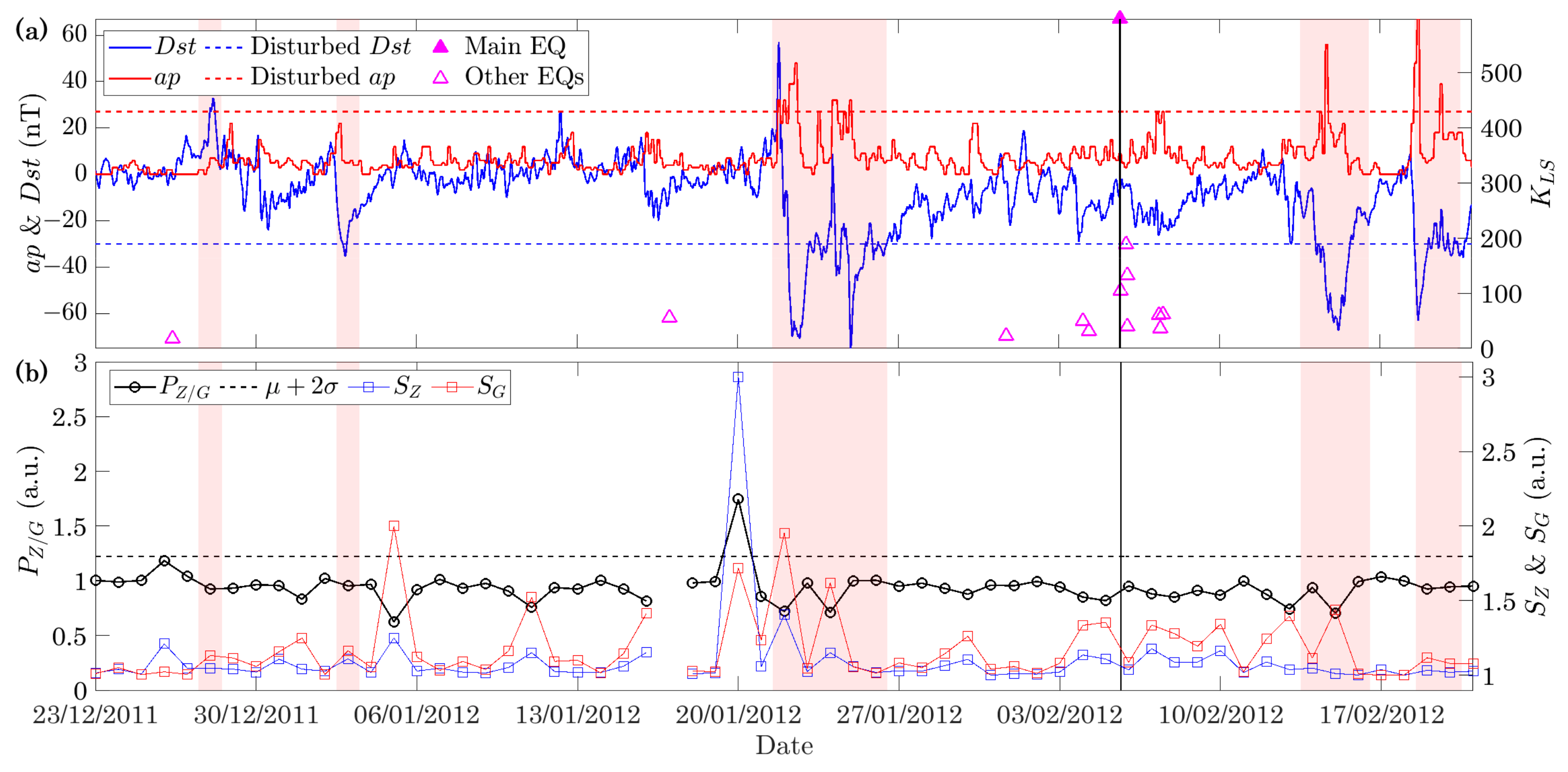
3.1. Precusor Detection

The polarization ratio analysis (PRA) method was first introduced by Hayakawa et al. [32]. The analysis was performed by calculating the ratio of power spectral density (PSD) of vertical (Z) to the PSD of total horizontal (G) field components by using the following formula:
P Z / G f = S Z f Δ f , Δ T S G f Δ f , Δ T
where P Z / G is the daily polarization ratio which is taken as the precursory parameter. In the equation, S Z and S G are the PSDs of vertical and total horizontal (G = H 2   +   D 2 ) components respectively, averaged over a ULF frequency range, Δf and over a local nighttime period, ∆T. This step was to minimize human-made noise during the day. Frequency ranges, Δf in prior studies were arbitrarily chosen [33], hence nine ranges were tested to determine the most effective one for each earthquake: Δf = 0.01–0.02, 0.02–0.03, …, 0.09–0.10 Hz. Similarly, nighttime period, ΔT, also differed across studies; thus, five different periods (ΔT = 22–02, 23–03, 00–04, 01–05 and 02–06 LT) were examined for each earthquake to identify the least geomagnetically disturbed period at which precursors appeared.
An anomaly is identified when the P Z / G value of a particular day exceeds the mean plus two times the standard deviation (μ + 2σ) of the entire period of observation [15]. If the anomaly appeared during an undisturbed period, then the anomaly was assumed to be a possible precursor. Some earthquakes were preceded by several anomalies in multiple Δf or/and ΔT; for these cases, the anomaly having the prominently highest amplitude was regarded as the precursor to the corresponding earthquake. Additionally, it is imperative to check that any increment of P Z / G is due to the significant increase of S Z and not the decrease of S G ; the observations of individual S Z and S G are useful for this purpose.
The PRA method has been improved over the years by employing various signal processing techniques such as standardization [34], and fractal dimension [35]. In this study, the method was further improved by introducing a new range-normalization process since means and standard deviations of both components are not directly comparable. After evaluating several range combinations heuristically, it was decided to normalize S G into the range [1,2] (between 1 and 2), and S Z into [1,3] (between 1 and 3) to give a greater weightage to the Z component, since it is the primary indicator of pre-earthquake anomalies. In addition to the μ + 2σ threshold value, the value of P Z / G must also exceed 1.5 to be considered as an anomaly. This is to ensure the reliability of the P Z / G parameter which requires the normalized value of S Z to be the maximum ( S Z , max   =   3 ) or one of the maximal values so that, when it is divided by any value of S G , the resultant P Z / G value is maintained at 1.5 or higher. It was found that the combination of the normalization ranges and the newly proposed threshold value was an effective modification to the original PRA method in detecting possible precursors of multiple earthquakes in this study.

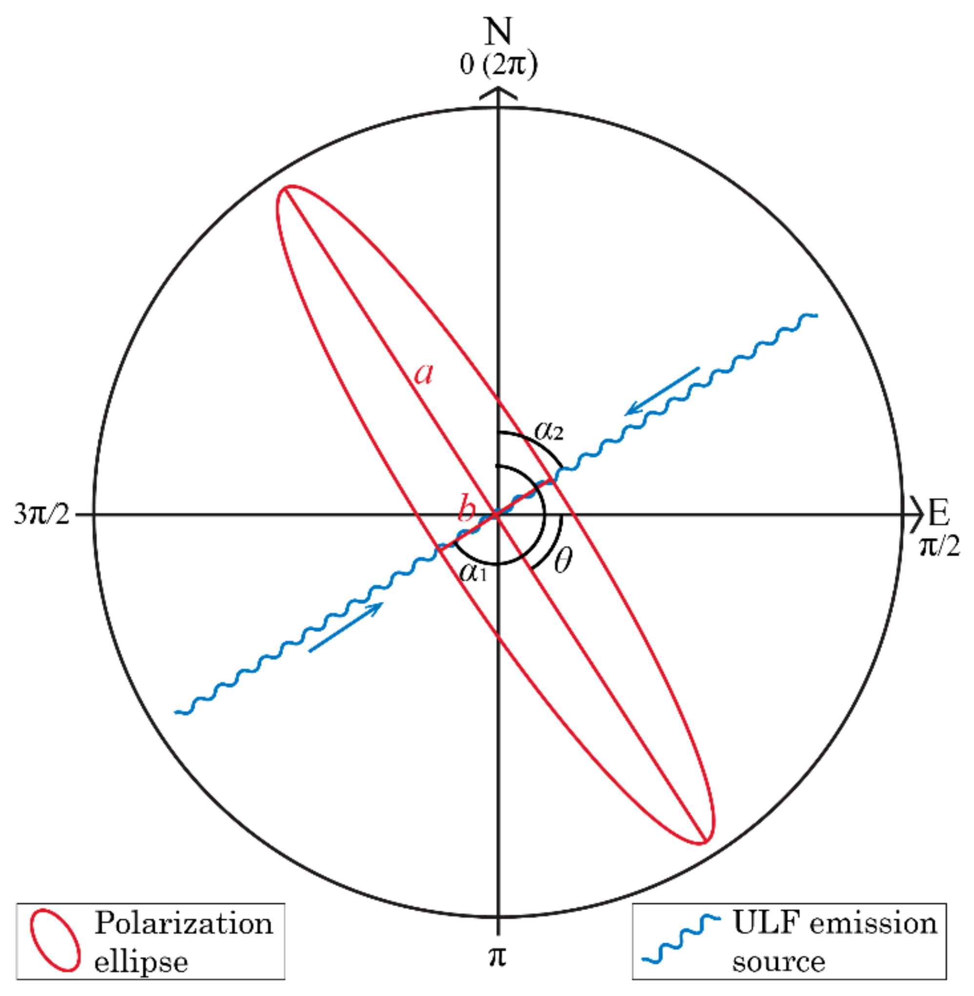
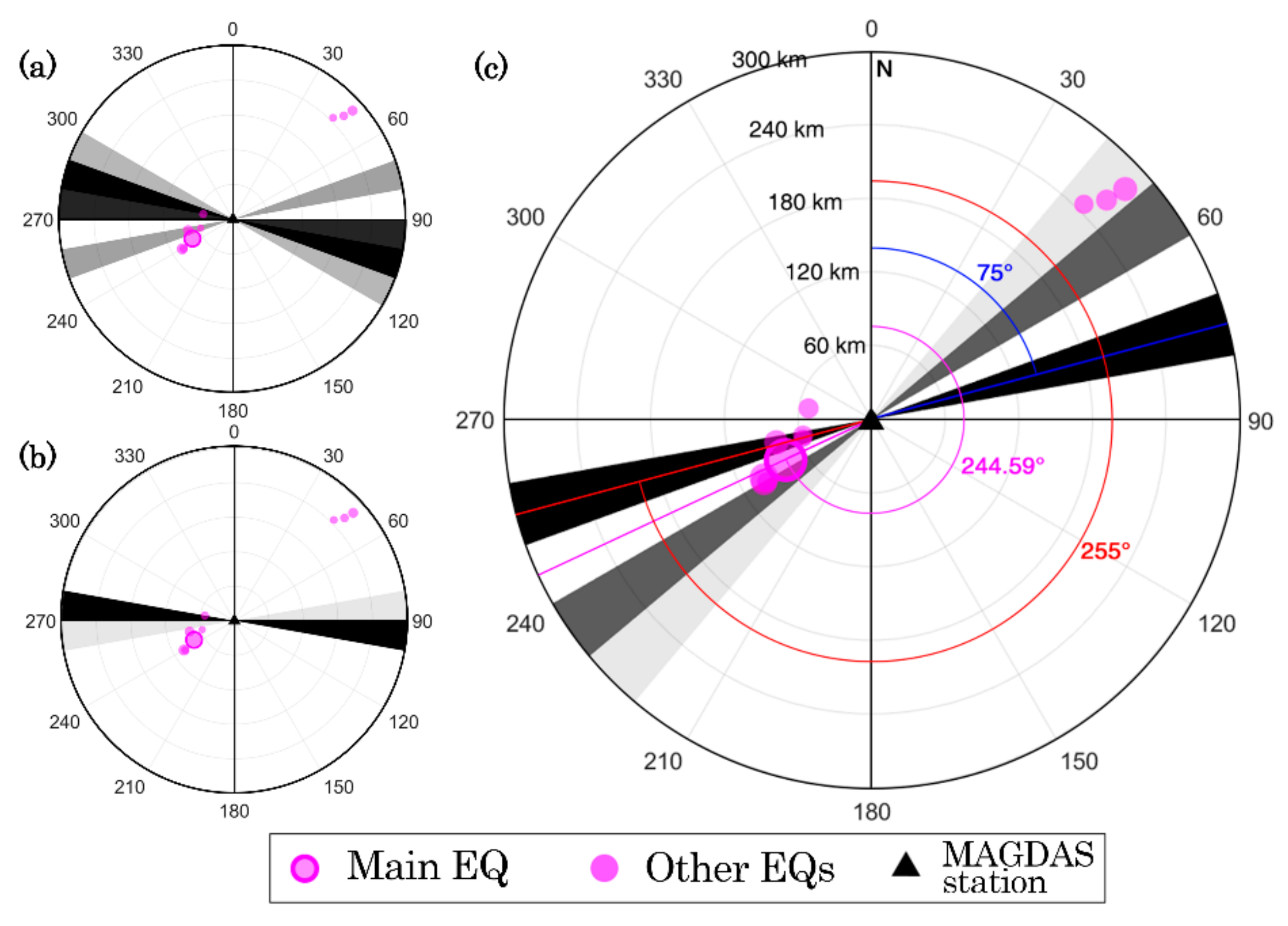
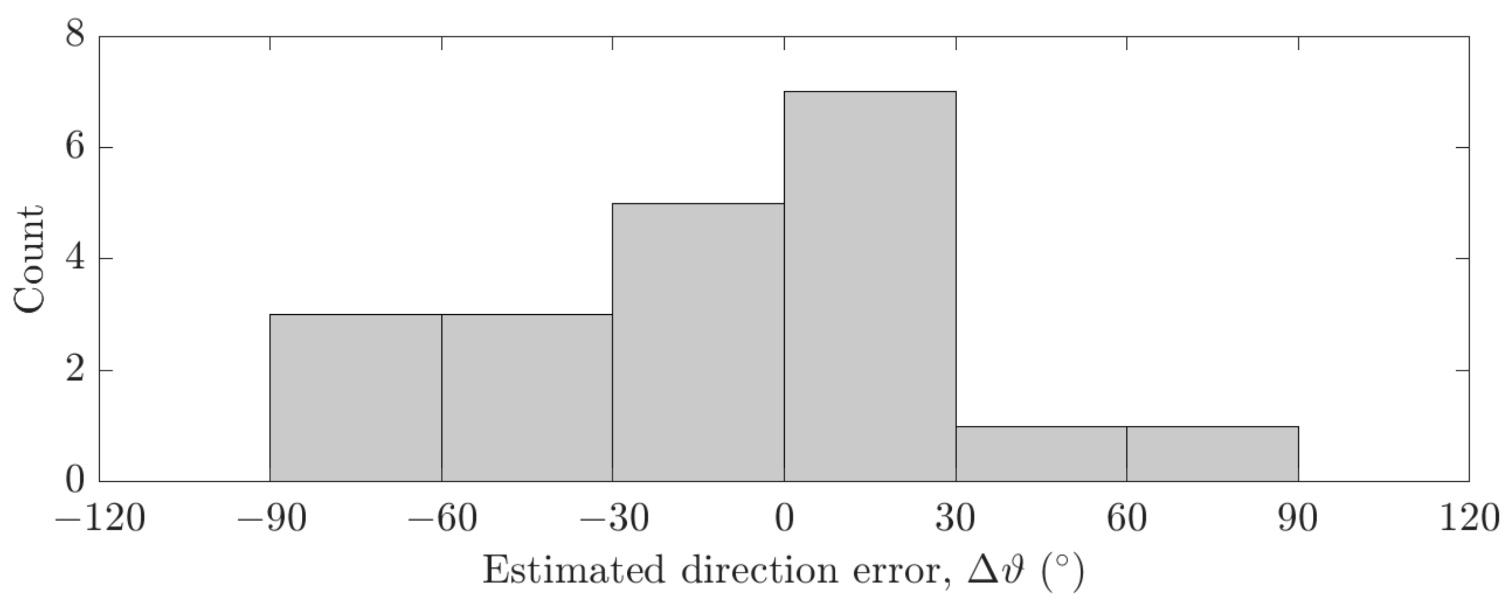
3.2. Direction Estimation

The polarization ellipse method used in this study was mainly based on the description by Schekotov et al. [3] and Ohta et al. [20]. The major angle, θ, is the angle the major axis of polarization ellipse (red line marked by a in Figure 2) makes with the eastward axis (E) with θ   <   0 revolving counterclockwise; its tangent is given by:
tan ( 2 θ )   =   2 A h A d   cos ( φ h φ d )   A d 2 A h 2
The H (northward) and D (eastward) geomagnetic components were first bandpass filtered in a frequency band Δf (determined previously, specific to each earthquake) to obtain quasi-monochromatic signals in the ULF range, U h and U d , respectively. The signals then underwent Hilbert transform to acquire complex signals. From the real and imaginary parts of the complex signals, the instantaneous amplitudes ( A h , A d ) and phase angles ( φ h , φ d ) were calculated to be used in Equation (3) to obtain θ.
The seismo-atmospheric emission is assumed to propagate from two possible directions towards the center of the ellipse as shown by the blue arrows in Figure 2. The azimuthal direction of the emission source (wiggly blue lines in Figure 2) is perpendicular to the major axis, hence, the angle between the direction and the northward axis (N) in the clockwise direction can be obtained by Equation (4):
α 1   =   π     θ
α 2   =   α 1   +   π
where α 1 is the first possible azimuthal direction that exists in the interval of π / 2 ,   3 π / 2 . The second possible direction, α 2 , in the interval of 3 π / 2 , π / 2 was found by calculating the opposite direction of every α 1 using Equation (5). Both α 1 and α 2 were combined to obtain the complete α in the whole interval of 0 ,   2 π .
In order to ensure that the obtained azimuthal angles are reliable in estimating the source direction, only α ( i ) which satisfy the following condition were included in the final plotting of azimuth distribution [20]:
U h 2 ( i )   +   U d 2 ( i )   >   K U h 2   +   U d 2
In Equation (6), the left-hand side is the instantaneous total intensity of horizontal magnetic component while the right-hand side (excluding K coefficient) is its average intensity in a given day. K acts as the minimum requirement coefficient of signal-to-noise ratio, where K = 5 was adopted by prior studies. On the other hand, we found in this study through a heuristic technique that K = 3.5 provides reasonable direction estimations for multiple earthquakes in different regions.

4. Results and Discussion

4.1. Precursor Detection and Direction Estimation

In this section, the investigation of earthquake ID no. 1 is elaborated and shown in Figure 3 and Figure 4 to exemplify the results of precursor detection and direction estimation. For precursor detection, Figure 3b illustrates a typical observation of P Z / G temporal evolution (black solid line). Values of P Z / G from 45 days before until 15 days after the earthquake were observed to identify statistically significant anomalies. It is to be noted that some data gaps existed during the period of observation for several earthquakes; these gaps are shown by disconnections of line, for example on 17th January 2012. As mentioned previously, the P Z / G parameter value must simultaneously exceed (i) μ   +   2 σ (black dashed line), and (ii) 1.5, to be considered as an anomaly. In this example, P Z / G (∆f = 0.01–0.02 Hz, ∆T = 01–05 LT) at CEB station satisfied both conditions on 20th January 2012 in the absence of geomagnetic storm and disturbance, where ap and Dst indices in Figure 3a are less than 27 nT and more than −30 nT respectively. During the date, S Z (blue line in Figure 3b) reached the maximum value of 3; meanwhile, S G (red line) remained at a moderate value of 1.718, thus verifying that the anomaly was due to a severe disturbance in the vertical component. This observation aligns with the premise of the PRA method which assumes that seismo-EM emission is more dominant in the vertical component. Therefore, the anomalous deviation can be assumed as the precursor for the 6th February 2012 M6.7 earthquake; the earthquake is represented by the filled magenta triangle symbol in Figure 3a.
The direction of the ULF emission source on the date of the precursor appearance was estimated for each earthquake. The ‘azimuthal beams’ at Cebu (CEB) station on 20 January 2012 is shown in Figure 4c as an example. The so-called azimuthal beam was obtained by classifying the azimuthal angle, α , into 36 sectors around the station; each sector is 10° wide. In Figure 4c, the darkness of the azimuthal beam represents the number of α falling into that beam; hence, the maximal beams (the darkest) are the most probable directions of the emission source. For each beam, there is an opposite beam, therefore, the maximal beam nearer to the earthquake of interest (outlined magenta circle in Figure 4c) is considered the final estimated direction. Also, the angle which the estimated direction makes with the true North in the clockwise direction is called the estimated azimuthal angle, ϑ . As illustrated in Figure 4c, there were two possible ϑ ’s: 75° (blue) and 255° (red); since ϑ = 255° is nearer to the earthquake of interest, it is taken as the only ϑ.
The azimuthal beams on the day before (19 January 2012) and the day after (21 January 2012) the date of precursor appearance are also shown in Figure 4a and Figure 4b, respectively, to illustrate the background polarization angle, which is influenced by the local electromagnetic condition and underground electrical composition. The maximal beams on 19 January 2012 pointed to 105°/285°; meanwhile the beams pointed to 95°/275° on 21 January 2012. This observation suggests that 95°–105°/275°–285° were the predominant azimuths of the normal background disturbance, thus the departure from these ranges on 20 January 2012 (Figure 4c) was possibly contributed by external influences such as local lithospheric process related to earthquake.
In order to evaluate the performance of the direction estimation, the error in degree and percentage ( Δ ϑ and Δ ϑ % , respectively) were calculated using the following formulae:
Δ ϑ   =   ϑ EQ ϑ ,   Δ ϑ % = Δ ϑ 360 °   ×   100 %
where ϑ EQ is the actual azimuthal angle of the earthquake epicenter as listed in Table 2 ( ϑ EQ = 244.59 in this example). By using Equation (7), we obtained that Δ ϑ and Δ ϑ % of earthquake no. 1 equals 10.41° and 2.892%, respectively. The same calculations were computed for other earthquakes. The histogram of estimated direction error, Δ ϑ , is illustrated in Figure 5 (the values are listed in Table 3), which shows that the majority of Δ ϑ s fall within ± 30 ° indicating that the estimations are sufficiently good with minimal error. The results might also support the association of the ULF emission with the corresponding earthquake.
A total of 20 out of 34 earthquakes (58.82%) were preceded by possible precursors. Four precursor characteristics were recorded in Table 3, which are the amplitude of precursor (A), frequency range (∆f), lead time ( τ , i.e., the number of days before the earthquake when the precursor appeared) and percentage error of estimated direction ( Δ ϑ % ). Additionally, the values of ap and Dst indices during the appearances of the precursor did not exceed the thresholds mentioned in Section 2, indicating that the global geomagnetic activities were low (see Table 3). Earthquake no. 18 which is the 2011 M9.0 Tohoku earthquake was studied previously by Takla et al. [36] in a similar manner in terms of the magnetometer station and method used. The results obtained in this study are in accord with those results regarding the lead time and frequency range. Meanwhile, the results for earthquake no. 10 are rather interesting since τ   =   0 days was observed, indicating that the precursor appeared on the same day as the earthquake occurrence. Upon closer inspection, it was revealed that the precursor was caused by a disturbance appearing in filtered ( Δ f   =   0.03 0.04   Hz ) Z and G components simultaneously 36 s after the earthquake, suggesting that the precursor is a result of co-seismic effect.
The modified PRA method was validated by performing the superposed epoch analysis (SEA) on the geomagnetic field data during ‘no-earthquake’ periods to form the control group. The SEA is a statistical tool that effectively superposes multiple binary (true/false) time series observations to reveal periodicities or a temporal correlation in the data [37,38]. In order to perform the analysis, we identified all 61-day periods of data measured by the 10 magnetometer stations (Table 1) throughout the years when no M     5.0 earthquakes occurred within 180 km from the stations. It was determined that 93 periods were available for the analysis, for which the data were subjected to the modified PRA method as described in Section 3.1. Since the nine frequency ranges, Δ f and five local nighttime periods, Δ T are characteristically unique, a total of 4185 (= 93   ×   9   ×   5 ) P Z / G temporal evolutions were obtained. The number of anomalies during geomagnetically undisturbed days were counted in each evolution and then added together. Figure 6 shows the results as a percentage, divided by the total number of observations ( n   =   4185 ) so that it can be compared with the percentage of precursor detection during the presence of earthquakes (i.e., the test group). The anomalies which appeared in the control group were less than 0.90 % per day throughout the 61-day period with no apparent trend, which suggests that the anomalies were probably random. In total, 5.87% of the observation periods in the control group contained at least one anomaly, which is significantly lower than 58.82% that was observed in the test group. It is concluded that the SEA results provide statistical validity of the modified PRA method in detecting possible earthquake precursors.

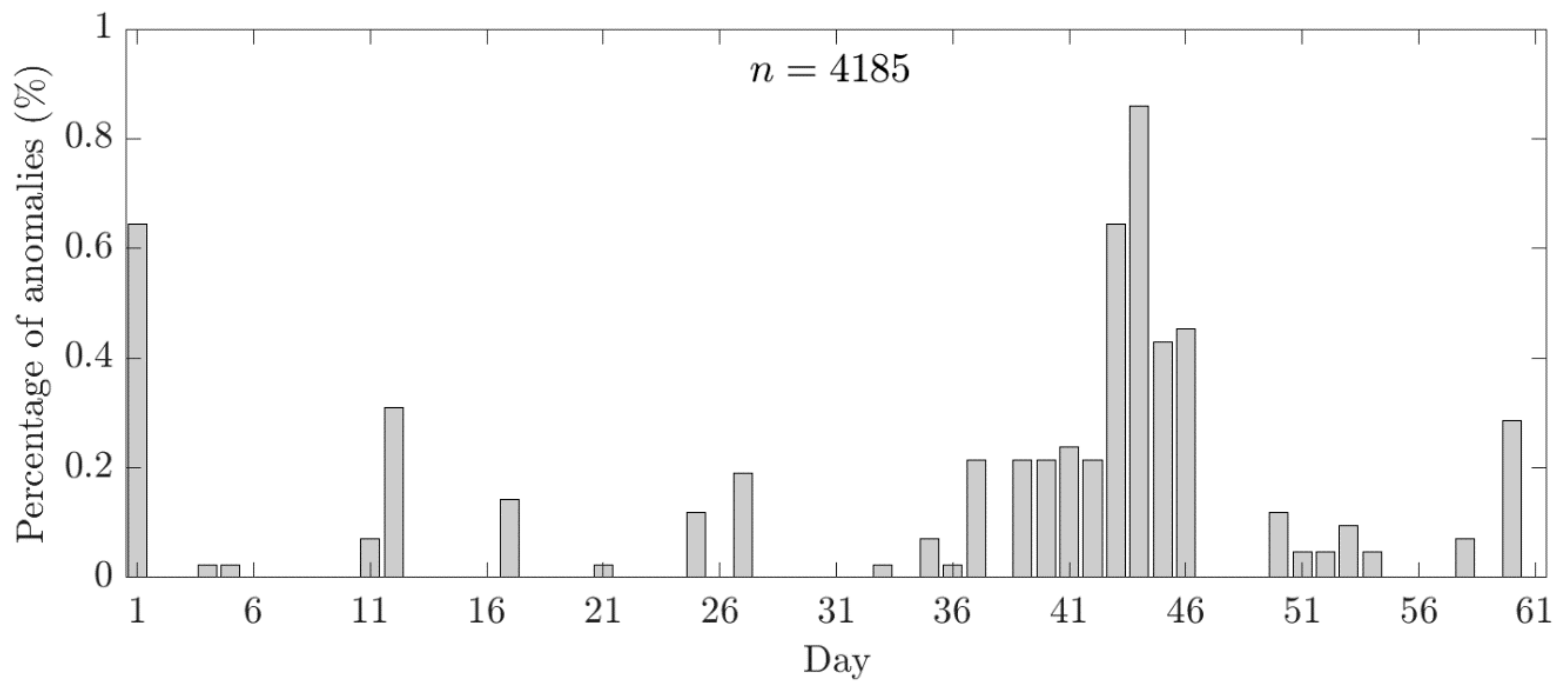
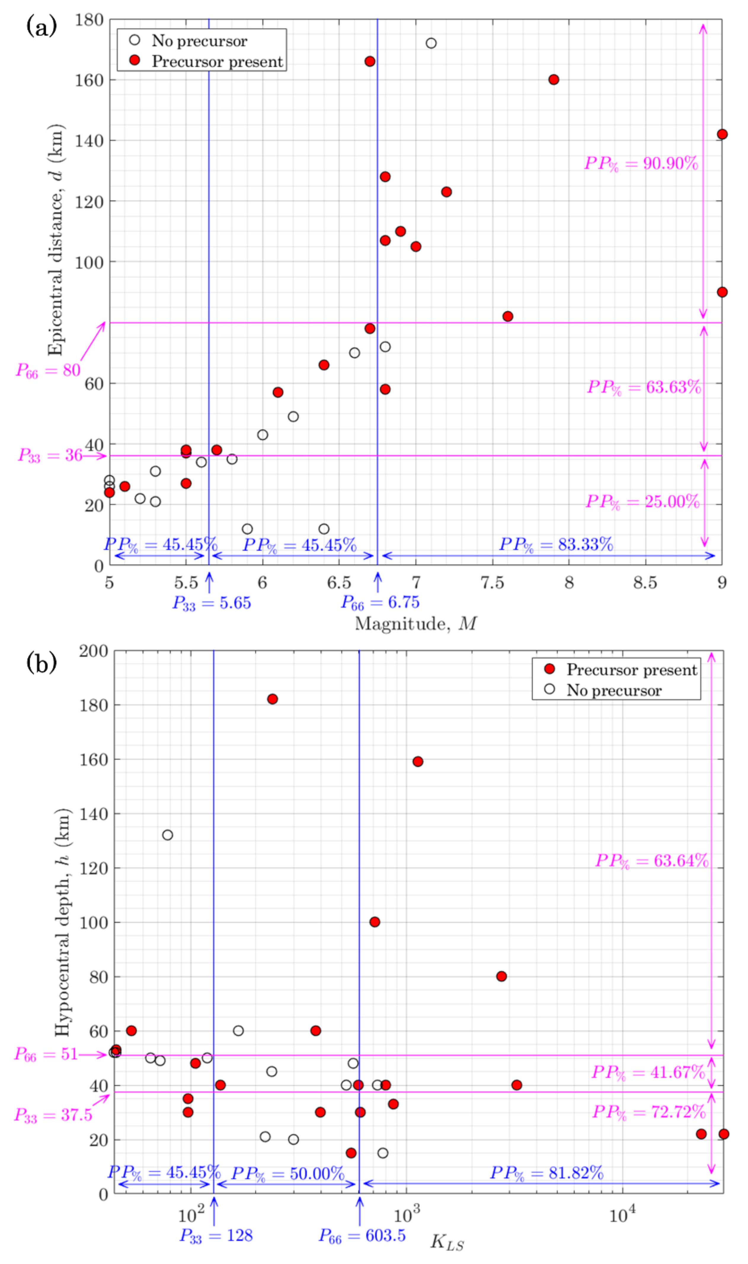
4.2. Statistics of Precursor Presences

A statistical analysis was performed to observe any dependence of precursor presences on different earthquake properties. Grouping earthquakes based on equal-width class intervals (e.g., M5.0–5.9, M6.0–6.9, etc.) will result in groups of unequal size and may cause biases when calculating percentage of precursor presences ( PP % ). Therefore, grouping based on percentile ranks, where earthquakes were divided into three equally sized groups based on their value ranks in terms of all four properties, yields a more accurate statistical representation.
Figure 7 shows the distribution of earthquakes that were and were not preceded by precursors (red and white circles respectively) by plotting their epicentral distance, d, against magnitude, M in Figure 7a, and their hypocentral depth, h, against local seismicity index, K LS in Figure 7b. The blue vertical and magenta horizontal lines are the boundaries between the groups and are labelled with corresponding percentile values. The three groups are (i) the ‘bottom’ group—below the 33rd percentile ( P < 33 ), (ii) the ‘middle’ group—between the 33rd and 66th percentiles ( P 33 66 ), and (iii) the ‘top’ group—above the 66th percentile ( P > 66 ).
From Figure 7a, it is apparent that PP % is the highest for both M and d in their respective top groups, where PP %   =   83.33 % and 90.91%, respectively. The observation regarding M aligns with the assumption that greater-magnitude earthquakes (which also have greater seismicity energy, indicated by higher K LS values) emit higher intensity of electromagnetic emission [3]. This high-intensity emission has a higher chance of being detected by magnetometer stations in the form of geomagnetic variation, thus increasing PP % . On the other hand, the high PP % for more distant earthquakes (indicated by higher d) seems to not agree with previous studies that have been summarized by Hayakawa [25]. However, this observation can be explained by the fact that most earthquakes having higher d in this study coincidentally have higher M, as illustrated in Figure 7a. The same explanation is applicable for the K LS against h plot in Figure 7b, where the majority of deeper earthquakes (higher h) have higher K LS ( K LS grows exponentially with M, see Equation (1)). From this statistical analysis, it is deduced that M and K LS are pivotal properties in determining the presence of precursors. For an earthquake having M   >   6.7 or/and K LS   >   ~ 600 , there was an approximately 80% chance of it being preceded by a precursor. Meanwhile, in order to infer the influences of h and d on PP % , a dataset containing earthquakes having similar M and K LS will be required.

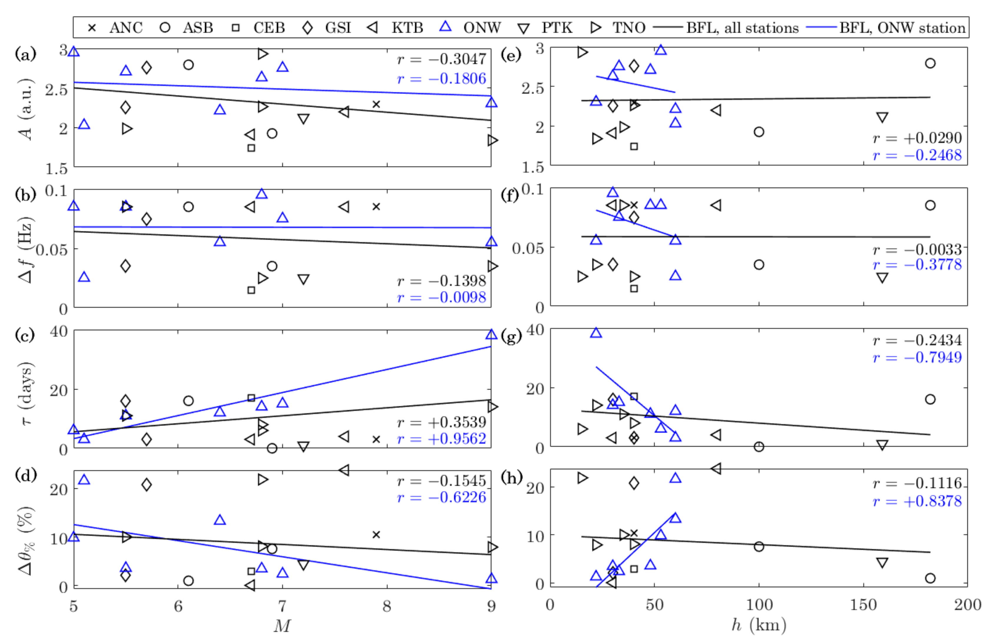
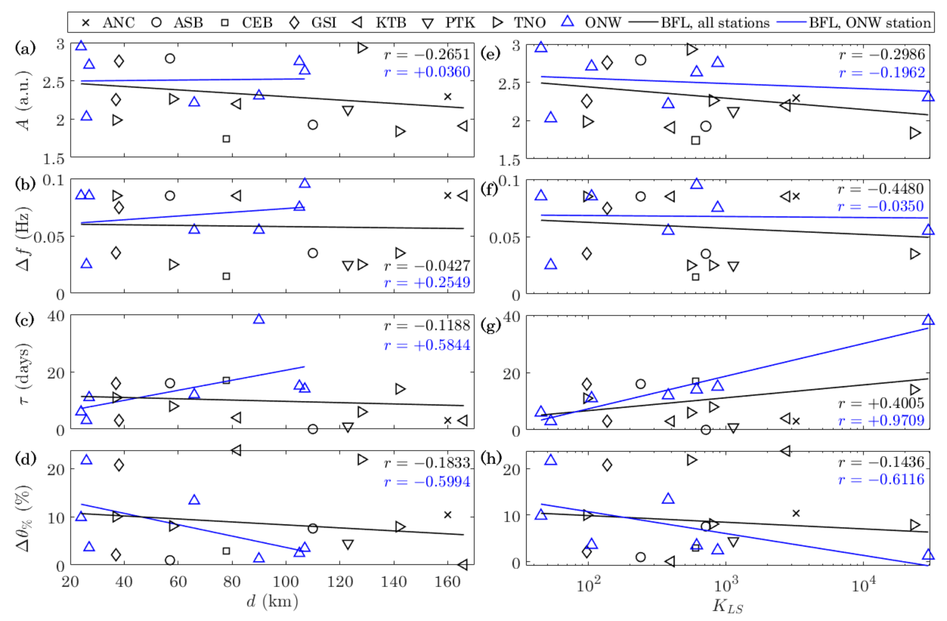
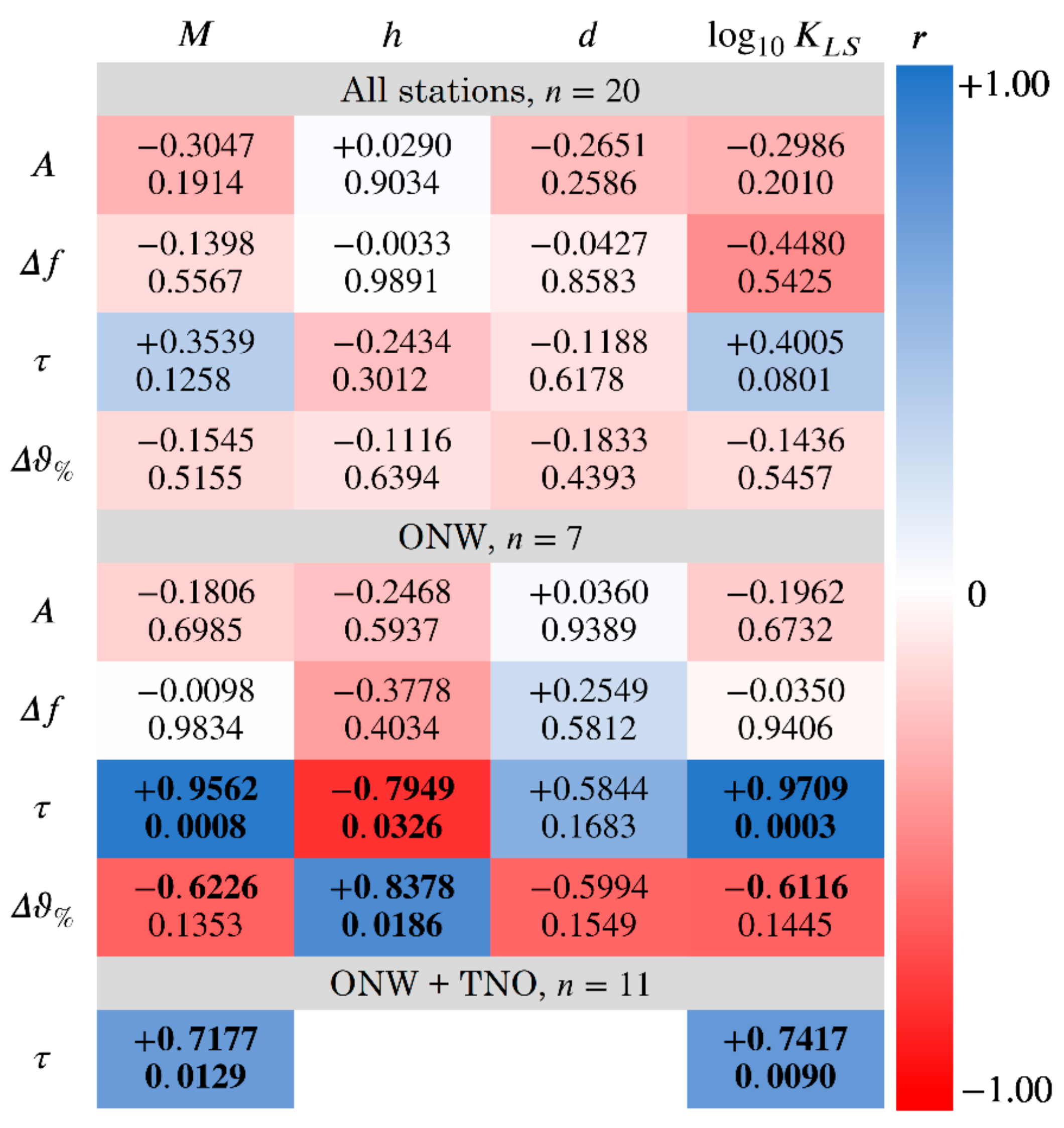
4.3. Correlation Analysis

Since precursors show varying characteristics across different earthquakes, they might possess correlations with the earthquake properties. Therefore, scatter plots of four precursor characteristics (A, Δf, τ and Δ ϑ % ) against four earthquake properties (M, h, d and K LS ) are shown in Figure 8 and Figure 9. The Pearson correlation coefficient, r, was calculated and written in black in the respective subfigure to identify which characteristic–property pairs have strong correlations, together with corresponding best-fit lines. The values of r were interpreted by following the characterizations for correlation strength suggested by Evans [39]: 0.00–0.19 (very weak), 0.20–0.39 (weak), 0.40–0.59 (moderate), 0.60–0.79 (strong) and 0.80–1.00 (very strong). In addition, the corresponding p-value less than 0.05 ( p   <   0.05 ) is considered statistically significant for the null hypothesis (that there is no correlation) to be rejected.
The r values (written in black) were obtained when data points from all stations were included, ranging from | r | =   0.0033 to 0.4480, which show very weak to moderate correlations. These generally weak correlations suggest that there could be a local dependence that affects the characteristics of found precursors. This dependence might be caused by the influences of the observatory station locations on the geomagnetic field components. For instance, a station near the magnetic equator would record a weaker intensity vertical component and stronger horizontal component while a station near the magnetic poles would record contrasting observations. Since the ONW station has the most data points, it was used to see if stronger correlations are exhibited when using data points from this station only; these data points are shown by the blue upright triangles in Figure 8 and Figure 9. Similarly, r values are included in each subfigure, written in blue. We paid attention to the | r |     0.60 to observe strong or very strong correlations.
The value of r   =   + 0.9562 (very strong) was observed for the τM pair (Figure 8c). The positive correlation value suggests that, for greater magnitude earthquakes, the lead time is longer (precursors appear earlier), which corresponds to the study by Ahadi et al. [22]. Similarly, K LS also showed a positive correlation with τ and had r = +0.9709 (very strong), which is the highest, where τ was shown to be longer for higher K LS (Figure 9g). These observations might be due to the greater strain energy accumulated at the focal region, where even if a fraction of this energy is converted into electromagnetic energy, it is sufficiently high to be detected by a near station at any point in time [21]. It is to be noted that the linear correlation between τ K LS was observed when K LS was scaled logarithmically (due to the positively skewed, heavy-tailed data distribution), which means that the correlation actually corresponds to τ log 10 K LS .
Hypocentral depth, h exhibits two correlations, namely with τ and Δ ϑ % , with r   =   0.7949 (strong) and +0.8378 (very strong) respectively. The τh pair (Figure 8g) exhibits a negative correlation which agrees with Ahadi et al. [22], i.e., for earthquakes with hypocenter located deeper underground, the precursor appears later than shallower ones. Additionally, it was shown from Δ ϑ % h correlation (Figure 8h) that the estimated azimuthal direction tends to have a larger error when the hypocentral depth is greater. This finding also means that shallower earthquakes produce higher reliability of direction estimation, thus offering advantages for the potential victims since shallower earthquakes are typically more destructive. There are other pairs which showed | r |     0.60 ; however, their respective p-values did not satisfy the p   <   0.05 condition.
Figure 10 shows a heatmap visualization of how r (the first number in each box) and p-value (the second number) differ across the properties and characteristics. In addition to all stations and ONW station data points, we also analyzed ONW+TNO stations combination, since the stations are just 100 km apart and located on the same tectonic plate, i.e., Okhotsk plate, hence the earthquake precursors detected in these stations might have similar characteristics. It was found that the correlations between τM and τ log 10 K LS continued to be strong, with r = +0.7177 and +0.7417 respectively (the last row in Figure 10). Besides, lead time, τ is more frequently correlated with earthquake properties than other precursor characteristics, which suggests that it is a dependent characteristic and rendering it useful in predicting the properties of upcoming earthquakes. It is worth mentioning that a finding by Chauhan et al. [21] which mentions a high correlation between Ad, and another finding regarding A K LS by Schekotov et al. [3], were not observed in this study. It is to note that Schekotov et al. [3] analyzed a different parameter (i.e., ULF depression), therefore their results might be incomparable with those obtained in this study.

5. Conclusions

In this paper, the correlations between four characteristics of possible geomagnetic precursor (amplitude, A, frequency, Δf, lead time, τ and percentage error of estimated direction, Δ ϑ % ) and four earthquake properties (magnitude, M, hypocentral depth, h, epicentral distance, d, and local seismicity index, K LS ) have been examined by utilizing vast MAGDAS geomagnetic field data on 34 earthquakes. In achieving the main objective, this study has improved the polarization ratio analysis (PRA) method (for precursor detection) by introducing a new normalization process with the following range combination: S Z   =   [ 1 ,   3 ] and S G   =   [ 1 ,   2 ] , while the polarization ellipse method (for direction estimation) has been successfully applied on a ULF range (0.01–0.10 Hz). As a result, 20 possible precursors were found (58.82% detection rate) and characterized. The detection rate is significantly higher than the percentage of anomalies observed during no-earthquake periods (5.87%), suggesting that the detected precursors were not by chance. The percentage of precursor presences was around 80% for earthquakes having M   >   6.7 and/or K LS   >   ~ 600 . The correlation strengths for all stations’ data points were found to be very weak to moderate. In contrast, the analysis of the Onagawa, Japan (ONW) station data points showed four pairs with strong to very strong linear correlations: (i) τ log 10 K LS ( r   =   + 0.9709 ), (ii) τM ( r   =   + 0.9562 ), (iii) Δ ϑ % h ( r   =   + 0.8378 ), and (iv) τh ( r   =   0.7949 ). Additionally, strong correlations were maintained for τ log 10 K LS ( r   =   + 0.7417 ) and τM ( r   =   + 0.7177 ) when the data points from ONW were combined with those from a near station, i.e., Tohno, Japan (TNO). In conclusion, some earthquake properties are strongly correlated with several precursor characteristics. However, the characteristics are locally dependent and exhibit heterogeneity, which is evidenced by the weak correlations for all stations data, but strong correlations for a single station data. It is recommended that more earthquakes having uniform distribution of properties be studied, in order to possibly discover more appreciable correlations.

Author Contributions

Conceptualization, K.A.Y., M.A., N.S.A.H. and S.A.; Data curation, A.Y.; Funding acquisition, M.A. and N.S.A.H.; Investigation, K.A.Y.; Methodology, K.A.Y., M.A., N.S.A.H. and S.A.; Project administration, M.A. and N.S.A.H.; Resources, A.Y.; Supervision, M.A., N.S.A.H. and S.A.; Visualization, K.A.Y.; Writing—original draft, K.A.Y.; Writing—review & editing, M.A., N.S.A.H. and S.A. All authors have read and agreed to the published version of the manuscript.

Funding

This research is supported by the grant FRGS/1/2020/TK0/UKM/01/1 of Ministry of Higher Education Malaysia. The work of A.Y. is supported by JSPS KAKENHI Grant JP20H01961 and JP15H05815.

Institutional Review Board Statement

Not applicable.

Informed Consent Statement

Not applicable.

Data Availability Statement

MAGDAS geomagnetic field data are available on request from Akimasa Yoshikawa ([email protected]). Global geomagnetic indices and earthquake data are publicly available at www.omniweb.gsfc.nasa.gov and www.emsc-csem.org, respectively.

Acknowledgments

The authors are thankful to the International Center for Space Weather Science and Education, Kyushu University for providing MAGDAS geomagnetic field data.

Conflicts of Interest

The authors declare no conflict of interest.

References

  1. Potirakis, S.; Schekotov, A.; Contoyiannis, Y.; Balasis, G.; Koulouras, G.; Melis, N.; Boutsi, A.; Hayakawa, M.; Eftaxias, K.; Nomicos, C. On possible electromagnetic precursors to a significant earthquake (Mw = 6.3) occurred in Lesvos (Greece) on 12 June 2017. Entropy 2019, 21, 241. [Google Scholar] [CrossRef] [PubMed] [Green Version]
  2. Yusof, K.A.; Abdullah, M.; Hamid, N.S.A.; Ahadi, S.; Yoshikawa, A. Normalized polarization ratio analysis for ULF precursor detection of the 2009 M7.6 Sumatra and 2015 M6.8 Honshu earthquakes. J. Kejuruteraan 2020, 3, 35–41. [Google Scholar] [CrossRef]
  3. Schekotov, A.; Chebrov, D.; Hayakawa, M.; Belyaev, G.G.; Berseneva, N. Short-term earthquake prediction in Kamchatka using low-frequency magnetic fields. Nat. Hazards 2020, 100, 735–755. [Google Scholar] [CrossRef]
  4. Molchanov, O.A.; Hayakawa, M. On the generation mechanism of ULF seismogenic electromagnetic emissions. Phys. Earth Planet. Inter. 1998, 105, 201–210. [Google Scholar] [CrossRef]
  5. Fedorov, E.N.; Pilipenko, V.; Uyeda, S. Electric and magnetic fields generated by electrokinetic processes in a conductive crust. Phys. Chem. Earth Part C 2001, 26, 793–799. [Google Scholar] [CrossRef]
  6. Sorokin, V.M.; Pokhotelov, O.A. Generation of ULF geomagnetic pulsations during early stage of earthquake preparation. J. Atmos. Sol. Terr. Phy. 2010, 72, 763–766. [Google Scholar] [CrossRef]
  7. Yamazaki, K. Temporal variations in magnetic signals generated by the piezomagnetic effect for dislocation sources in a uniform medium. Geophys. J. Int. 2016, 206, 130–141. [Google Scholar] [CrossRef]
  8. Dudkin, F.; Korepanov, V.; Yang, D.; Li, Q.; Leontyeva, O. Analysis of the local lithospheric magnetic activity before and after Panzhihua Mw = 6.0 earthquake (30 August 2008, China). Nat. Hazards Earth Syst. Sci. 2011, 11, 3171–3180. [Google Scholar] [CrossRef]
  9. Prattes, G.; Schwingenschuh, K.; Eichelberger, H.U.; Magnes, W.; Boudjada, M.; Stachel, M.; Vellante, M.; Villante, U.; Wesztergom, V.; Nenovski, P. Ultra Low Frequency (ULF) European multi station magnetic field analysis before and during the 2009 earthquake at L’Aquila regarding regional geotechnical information. Nat. Hazards Earth Syst. Sci. 2011, 11, 1959–1968. [Google Scholar] [CrossRef] [Green Version]
  10. Siingh, D.; Singh, A.K.; Patel, R.P.; Singh, R.; Singh, R.P.; Veenadhari, B.; Mukherjee, M. Thunderstorms, lightning, sprites and magnetospheric whistler-mode radio waves. Surv. Geophys. 2008, 29, 499–551. [Google Scholar] [CrossRef] [Green Version]
  11. Berthelier, J.-J.; Malingre, M.; Pfaff, R.; Seran, E.; Pottelette, R.; Jasperse, J.; Lebreton, J.-P.; Parrot, M. Lightning-induced plasma turbulence and ion heating in equatorial ionospheric depletions. Nat. Geosci. 2008, 1, 101–105. [Google Scholar] [CrossRef]
  12. Rietveld, M.T.; Stubbe, P.; Kopka, H. On the frequency dependence of ELF/VLF waves produced by modulated ionospheric heating. Radio Sci. 1989, 24, 270–278. [Google Scholar] [CrossRef]
  13. Papadopoulos, K. The magnetic response of the ionosphere to pulsed HF heating. Geophys. Res. Lett. 2005, 32. [Google Scholar] [CrossRef]
  14. Stanica, D.A.; Stanica, D. ULF pre-seismic geomagnetic anomalous signal related to Mw8.1 offshore Chiapas earthquake, Mexico on 8 September 2017. Entropy 2019, 21, 29. [Google Scholar] [CrossRef] [PubMed] [Green Version]
  15. Yusof, K.A.; Hamid, N.S.A.; Abdullah, M.; Ahadi, S.; Yoshikawa, A. Assessment of signal processing methods for geomagnetic precursor of the 2012 M6.9 Visayas, Philippines earthquake. Acta Geophys. 2019, 142, 1297–1306. [Google Scholar] [CrossRef]
  16. Hirano, T.; Hattori, K. ULF geomagnetic changes possibly associated with the 2008 Iwate–Miyagi Nairiku earthquake. J. Asian Earth Sci. 2011, 41, 442–449. [Google Scholar] [CrossRef]
  17. Masci, F. Comment on “Ultra Low Frequency (ULF) European multi station magnetic field analysis before and during the 2009 earthquake at L’Aquila regarding regional geotechnical information” by Prattes et al. (2011). Nat. Hazards Earth Syst. Sci. 2012, 12, 1717–1719. [Google Scholar] [CrossRef] [Green Version]
  18. Masci, F.; Thomas, J.N. Are there new findings in the search for ULF magnetic precursors to earthquakes? J. Geophys. Res. 2015, 120, 10289–10304. [Google Scholar] [CrossRef] [Green Version]
  19. Potirakis, S.; Hayakawa, M.; Schekotov, A. Fractal analysis of the ground-recorded ULF magnetic fields prior to the 11 March 2011 Tohoku earthquake (Mw=9): Discriminating possible earthquake precursors from space-sourced disturbances. Nat. Hazards 2017, 85, 59–86. [Google Scholar] [CrossRef]
  20. Ohta, K.; Izutsu, J.; Schekotov, A.; Hayakawa, M. The ULF/ELF electromagnetic radiation before the 11 March 2011 Japanese earthquake. Radio Sci. 2013, 48, 589–596. [Google Scholar] [CrossRef]
  21. Chauhan, V.; Singh, O.P.; Pandey, U.; Singh, B.; Arora, B.R.; Rawat, G.; Pathan, B.M.; Sinha, A.K.; Sharma, A.K.; Patil, A.V. A search for precursor of earthquakes from multi-station ULF observation and TEC measurements in India. Indian J. Radio Space 2012, 41, 543–556. [Google Scholar]
  22. Ahadi, S.; Puspito, T.; Ibrahim, G.; Saroso, S.; Yumoto, K.; Yoshikawa, A.; Muzli, M. Anomalous ULF emissions and their possible association with the strong earthquakes in Sumatra, Indonesia, during 2007–2012. J. Math. Fund. Sci. 2015, 47, 84–103. [Google Scholar] [CrossRef]
  23. Yumoto, K.; MAGDAS Group. Space weather activities at SERC for IHY: MAGDAS. Bull. Seismol. Soc. Am. 2007, 35, 511–522. [Google Scholar]
  24. Bello, S.A.; Abdullah, M.; Hamid, N.S.A.; Yoshikawa, A.; Olawepo, A.O. Variations of B0 and B1 with the solar quiet Sq-current system and comparison with IRI-2012 model at Ilorin. Adv. Space Res. 2017, 60, 307–316. [Google Scholar] [CrossRef]
  25. Hayakawa, M. Earthquake Prediction with Radio Techniques; John Wiley & Sons Pte Ltd.: Singapore, 2015; ISBN 1118770161. [Google Scholar]
  26. Molchanov, O.A.; Hayakawa, M. Seismo Electromagnetics and Related Phenomena: History and Latest Results; Terrapub: Tokyo, Japan, 2008; ISBN 978-4-88704-143-1. [Google Scholar]
  27. Rostoker, G. Geomagnetic indices. Rev. Geophys. 1972, 10, 935–950. [Google Scholar] [CrossRef]
  28. Namgaladze, A.; Karpov, M.; Knyazeva, M. Seismogenic disturbances of the ionosphere during high geomagnetic activity. Atmosphere 2019, 10, 359. [Google Scholar] [CrossRef] [Green Version]
  29. Gonzalez, W.D.; Joselyn, J.A.; Kamide, Y.; Kroehl, H.W.; Rostoker, G.; Tsurutani, B.T.; Vasyliunas, V.M. What is a geomagnetic storm? J. Geophys. Res. 1994, 99, 5771. [Google Scholar] [CrossRef]
  30. Yaso, N.; Hasbi, A.M.; Abdullah, M. Investigation of ionospheric and magnetic response during the 2011 Tohoku earthquake using ground based measurement. Indian J. Radio Space 2016, 45, 115–125. [Google Scholar]
  31. Hasbi, A.M.; Mohd Ali, M.A.; Misran, N. Ionospheric variations before some large earthquakes over Sumatra. Nat. Hazards Earth Syst. Sci. 2011, 11, 597–611. [Google Scholar] [CrossRef]
  32. Hayakawa, M.; Kawate, R.; Molchanov, O.A.; Yumoto, K. Results of ultra-low-frequency magnetic field measurements during the Guam Earthquake of 8 August 1993. Geophys. Res. Lett. 1996, 23, 241–244. [Google Scholar] [CrossRef]
  33. Yusof, K.A.; Abdullah, M.; Hamid, N.S.A.; Ahadi, S. On effective ULF frequency ranges for geomagnetic earthquake precursor. In Proceedings of the International Conference on Space Weather and Satellite Application (ICeSSAT 2018), UiTM Shah Alam, Selangor, Malaysia, 7–9 August 2019; Jusoh, M.H., Yaacob, N., Radzi, Z.M., Manut, A., Eds.; IOP Science: Bristol, UK, 2019; pp. 1–8. [Google Scholar]
  34. Ida, Y.; Yang, D.; Li, Q.; Sun, H.; Hayakawa, M. Detection of ULF electromagnetic emissions as a precursor to an earthquake in China with an improved polarization analysis. Nat. Hazards Earth Syst. Sci. 2008, 8, 775–777. [Google Scholar] [CrossRef]
  35. Rawat, G.; Chauhan, V.; Dhamodharan, S. Fractal dimension variability in ULF magnetic field with reference to local earthquakes at MPGO, Ghuttu. Geomat. Nat. Hazards Risk 2016, 7, 1937–1947. [Google Scholar] [CrossRef] [Green Version]
  36. Takla, E.M.; Yumoto, K.; Okano, S.; Uozumi, T.; Abe, S. The signature of the 2011 Tohoku mega earthquake on the geomagnetic field measurements in Japan. NRIAG J. Astron. Geophys. 2013, 2, 185–195. [Google Scholar] [CrossRef] [Green Version]
  37. Singh, Y.P.; Badruddin. Statistical considerations in superposed epoch analysis and its applications in space research. J. Atmos. Sol. Terr. Phy. 2006, 68, 803–813. [Google Scholar] [CrossRef]
  38. Hattori, K.; Han, P.; Yoshino, C.; Febriani, F.; Yamaguchi, H.; Chen, C.-H. Investigation of ULF seismo-magnetic phenomena in Kanto, Japan during 2000–2010: Case studies and statistical studies. Surv. Geophys. 2013, 34, 293–316. [Google Scholar] [CrossRef]
  39. Evans, J.D. Straightforward Statistics for the Behavioral Sciences; Brooks/Cole: Pacific Grove, CA, USA, 1996; ISBN 9780534231002. [Google Scholar]
Figure 1. Maps of (a) South America, (b) East Asia, and (c) Southeast Asia. The circle radii are proportional to the magnitude of the earthquakes. The scale bar in (a) is relevant to the whole figure.
Universe 07 00020 g001
Figure 2. Illustration of the polarization ellipse and possible directions of the ultra-low frequency (ULF) emission source.
Universe 07 00020 g002
Figure 3. Temporal evolution of (a) ap & Dst indices (left axis) and K LS of nearby earthquakes (right axis), and (b) P Z / G parameter and its μ   +   2 σ threshold (left axis), and individual S Z and S G (right axis) at CEB station (December 2011–February 2012). Disturbed days, in which either ap or Dst exceeds their respective disturbed threshold, are shaded red.
Universe 07 00020 g003
Figure 4. Azimuthal beams at CEB station on (a) 19th January 2012, (b) 21st January 2012, and (c) 20 January 2012 (the date of the precursor appearance in Figure 3). The circle sizes indicate the magnitudes of the earthquake. In (c), the angles between the true North (N) and the earthquake of interest, the first ϑ , and the second ϑ are written in magenta, blue and red, respectively.
Universe 07 00020 g004
Figure 5. Histogram of estimated direction error, Δ ϑ . The relatively high counts near 0 ° indicate the estimations are good with minimal error.
Universe 07 00020 g005
Figure 6. Percentage of anomalies during no-earthquake (i.e., the control group) periods throughout 61 days of observation.
Universe 07 00020 g006
Figure 7. Distributions of precursor presences in terms of (a) epicentral distance, d against magnitude, M , and (b) hypocentral depth, h against K LS index. Earthquakes were divided into 3 groups based on their percentile ranks, i.e., P < 33 , P 33 66 and P > 66 . The percentage of precursor presences, PP % is shown for each group.
Universe 07 00020 g007
Figure 8. Scatter plots of amplitude (A), frequency (Δf), lead time (τ) and percentage of error ( Δ ϑ % ) against magnitude (M) in (ad), and against hypocentral depth (h) in (eh). Straight lines show best-fit lines (BFL) using all stations (black) and only ONW station data points (blue). Corresponding r values are written in the respective colors.
Universe 07 00020 g008
Figure 9. Similar to Figure 8, but for A, Δf, τ and Δ ϑ % against epicentral distance (d) in (ad); and against K LS in (eh) where logarithmic scale is used for x-axis.
Universe 07 00020 g009
Figure 10. Heat map of r (the first number in each box) for each property–characteristic pair using three data points: all stations, ONW station and ONW+TNO stations. Corresponding p-values are included (the second number). The values of | r |   0.60 and p   <   0.05 are emboldened.
Universe 07 00020 g010
Table 1. Magnetic Data Acquisition System (MAGDAS) station data used in this study.
RegionCodeLocationLat. (°N) 1Lon. (°E) 1Year (s) 2
Southeast AsiaCEBCebu, Philippines10.36123.912011–2012
CDOCagayan De Oro, Philippines8.46124.632013
GSIGunung Sitoli, Indonesia1.1897.342014–2015
KTBKotatabang, Indonesia−0.20100.322009
East AsiaPTKParatunka, Russia52.94158.252013, 2015–2016
ASBAshibetsu, Japan43.46142.172011–2013
TNOTohno, Japan39.30141.602011, 2013–2015
ONWOnagawa, Japan38.40141.472008, 2010–2013, 2015–2016
HLNHualien, Taiwan23.90121.552009–2013
South AmericaANCAncon, Peru−11.77−77.152007
1 Refer to geographic latitude and longitude respectively throughout this paper. 2 Refers to the year(s) for which data are available.
Table 2. Studied earthquakes and their properties.
ID 1Date (UT)Lat. (°N)Lon. (°E)M2h (km) 3Station 4d (km) 5 K LS   6 ϑ EQ (°) 7
16 February 201210.06123.276.740CEB78597244.59
215 October 201309.92124.107.115CDO172776340.33
314 September 201401.17097.275.530GSI3797247.25
48 May 201501.56097.805.740GSI3813740.22
516 August 2009−01.42099.466.730KTB166398215.17
630 September 2009−00.76099.847.680KTB822754220.60
726 February 201353.06158.015.3132PTK2178309.82
830 January 201654.03158.547.2159PTK12311288.88
921 October 201143.91142.516.1182ASB5723928.53
102 February 201342.79143.176.9100ASB110712132.21
1111 March 201138.30142.509.022TNO14223,214146.48
1231 March 201339.12141.885.535TNO3797138.97
1316 February 201539.87142.946.815TNO12855363.73
1412 May 201538.95141.996.840TNO58799144.12
151 June 200838.51141.775.160ONW265372.77
1613 June 200839.12140.647.033ONW105868316.34
1719 July 200837.63142.136.830ONW107610147.50
1811 March 201138.30142.509.022ONW9029,55499.61
1914 March 201037.82141.616.640ONW70525170.59
2025 January 201238.21141.695.349ONW3172144.32
218 March 201238.63141.665.052ONW264536.48
225 May 201238.25141.545.250ONW2265166.07
2317 June 201238.97141.836.460ONW6637927.15
2429 August 201238.49141.785.548ONW2710577.89
2525 October 201238.33141.845.650ONW34119111.18
2621 November 201238.55141.725.053ONW244559.57
2717 April 201338.53141.565.945ONW1223734.81
284 August 201338.26141.815.860ONW35166124.72
2912 May 201538.95141.996.840ONW7273237.81
3026 April 201638.22141.635.052ONW2844151.81
3119 December 200923.87121.666.448HLN12565106.59
3227 March 201323.84121.136.021HLN43221261.21
332 June 201323.79121.086.220HLN49299255.74
3415 August 2007−13.14−076.717.940ANC1603240162.64
1 Each earthquake is given an ID number. Meaning of the symbols: 2 magnitude of earthquake, 3 hypocentral depth, 4 observatory station (usually the nearest to the epicenter), 5 epicentral distance, 6 local seismicity index, and 7 the azimuthal angle of the earthquake epicenter in reference to the station.
Table 3. Characteristics of found precursors.
ID 1A (a.u.) 2Δf (Hz) 3 τ (Days) 4 Δ T   ( LT )   5 ϑ (°) 6 Δ ϑ   ( ° )   7 Δ ϑ %   ( % )   8 ap, Dst (nT) 9
11.7460.01–0.021701–05255−10.412.8925, −5
32.2540.03–0.041601–05255−7.752.15322, −26
42.7630.07–0.08322–02115−74.7820.7724, −9
51.9110.08–0.09300–042150.170.0473, −7
62.1990.08–0.09422–0213585.6023.7784, 11
82.1260.02–0.03102–0625−16.124.4783, −2
92.7930.08–0.091600–04253.530.98122, −23
101.9260.03–0.040 1022–0210527.217.5587, −18
111.8400.03–0.041400–04175−28.527.9224, 0
121.9870.08–0.091122–02175−36.0310.0089, −28
132.9320.02–0.03600–04345−78.7321.8696, −8
142.2640.02–0.03822–0211529.128.08912, −6
152.0290.02–0.03302–06355−77.7721.60312, −4
162.7520.07–0.081522–02325−8.662.40612, −11
172.6300.09–0.101423–0313512.503.47212, −10
182.3040.05–0.063800–04954.611.28118, −19
232.2130.05–0.061222–0275−47.8513.29227, −26
242.7060.08–0.091101–056512.893.58122, −6
262.9460.08–0.09600–0495−35.439.8423, −23
342.2980.08–0.09302–0612537.6410.4567, −18
1 The IDs match the earthquake IDs in Table 2 (IDs not listed indicate the absence of precursors). Meaning of the symbols: 2 amplitude, 3 frequency range, 4 lead time, 5 nighttime period, 6 estimated azimuthal angle, 7 estimated direction error, and 8 percentage error of the estimated direction. 9 Maximum ap and minimum Dst during the respective nighttime periods. 10 The precursor appeared on the same day of the earthquake event.
Publisher’s Note: MDPI stays neutral with regard to jurisdictional claims in published maps and institutional affiliations.

