
High-Order Multipole and Binary Love Number Universal Relations


1
Department of Physics, The Pennsylvania State University, University Park, PA 16802, USA
2
Institute for Gravitation & The Cosmos, The Pennsylvania State University, University Park, PA 16802, USA
3
Department of Astronomy & Astrophysics, The Pennsylvania State University, University Park, PA 16802, USA
*
Author to whom correspondence should be addressed.
Universe 2021, 7(10), 368; https://0-doi-org.brum.beds.ac.uk/10.3390/universe7100368
Submission received: 2 September 2021
/
Revised: 25 September 2021
/
Accepted: 29 September 2021
/
Published: 30 September 2021
/
Corrected: 23 November 2021
(This article belongs to the Special Issue Properties and Dynamics of Neutron Stars and Proto-Neutron Stars)
Abstract
:Using a data set of approximately 2 million phenomenological equations of state consistent with observational constraints, we construct new equation-of-state-insensitive universal relations that exist between the multipolar tidal deformability parameters of neutron stars, , for several high-order multipoles (), and we consider finite-size effects of these high-order multipoles in waveform modeling. We also confirm the existence of a universal relation between the radius of the NS, and the reduced tidal parameter of the binary, , and the chirp mass. We extend this relation to a large number of chirp masses and to the radii of isolated NSs of different mass M, . We find that there is an optimal value of M for every such that the uncertainty in the estimate of is minimized when using the relation. We discuss the utility and implications of these relations for the upcoming LIGO O4 run and third-generation detectors.
1. Introduction
Due to the constraints imposed by general relativity and causality, there exist quasi-universal relations between various bulk physical properties of neutron stars (NSs) that are mostly insensitive to the actual equation of state (EOS) of nuclear matter [1,2,3,4,5,6,7,8,9,10,11,12,13,14]. Since the nuclear EOS in the high-density regime of NSs is still unknown, these universal relations are a great utility for gravitational wave (GW) astronomy. Universal relations reduce a group of several seemingly independent physical properties to a family characterized by only a few parameters. Ideally, this allows one to break the degeneracies between parameters in the analysis of GW data as well as in waveform modelling.
A robust set of universal relations (called multipole Love relations) holds between the l-th order dimensionless gravitoelectric tidal deformability coefficients of NSs [12], , which are defined by
where is the compactness of the NS (here we take ) and is its l-th order gravitoelectric tidal Love number [15]. The GW waveform of a binary NS (BNS) merger is, quite understandably, highly sensitive to these tidal parameters. How deformable a NS is in a tidal potential affects how its mass ultimately gets distributed during the inspiral of a merger, which, in turn, shapes the GW waveform, especially during the late stages of the inspiral [15,16,17,18,19]. The tidal parameters enter into the waveform at different post-Newtonian orders; however, they are degenerate in the signal [12]. The multipole relations allow this degeneracy to be broken by reducing all of the tidal deformabilities to a family determined by a single parameter. This parameter is always chosen to be the quadrupolar tidal deformability , which is the source of the leading-order finite-size effect in the GW signal and, consequently, is the easiest to measure [12]. Thus, higher-order () tidal deformabilities can be expressed through the multipole Love relations as functions of . The authors and others have demonstrated that the improvements to the accuracy of tidal deformability measurements, to parameter estimation, and to GW modelling offered by the multipole Love relations are significant [12,14,15,20,21] and will become particularly important with the increased sensitivity of upcoming third-generation GW detectors like LIGO III, the Einstein Telescope, and Cosmic Explorer [12,15,22,23,24,25].
Motivated by these potential improvements, we present entirely new fits to several previously un-fitted high-order multipole Love relations, specifically for and 8. Though the finite-size effects of these orders of tidal parameters are currently smaller than measurement error, they will become more measurable with increased sensitivity; hence, faithful GW waveform modelling will need to incorporate them. Previosu studies, such as Flanagan and Hinderer [26] and Damour et al. [27], have discussed the finite-size effects of the multipoles.
Zhao and Lattimer [19], De et al. [28] have demonstrated the existence of an intriguing EOS-insensitive relation for BNSs between the radius of the NS, and the reduced tidal deformability (also called the binary tidal deformability), . The quadrupolar deformabilities of the individual NSs enter into the GW signal of the merger via , which is defined as
where and are the deformabilities of the primary and the secondary stars, respectively. The quadrupolar tidal Love number is known to scale roughly as independently of the EOS [15,29]. According to Equation (1), this means scales approximately as . In an apparently analogous fashion, seems to go as , where is the chirp mass of the BNS given by
Combining this observation with the definition of in the manner done by Zhao and Lattimer [19] yields a mostly EOS-insensitive estimate of in terms of and that is also mostly insensitive to the binary mass ratio q:
The immediate utility of this relation is the ability to produce an EOS-agnostic estimate of from just tidal parameter measurements. This is an alternative to the more involved method of using the universal relation for binaries between the symmetric and antisymmetric combinations of and [14,30] combined with the relation for individual NSs between and the compactness C [14,31] (a relation which intuitively follows from the definition of in Equation (1)). One would first use the symmetric-antisymmetric relation to break the degeneracy between and and estimate them individually from , and then use the -C relation and the masses of the binary to extract the radii of both stars. The LIGO/VIRGO analysis of GW170817 is an example of this latter approach [28,32,33]. One need not appeal to universal relations to estimate stellar radii, however. Instead, one could perform an inference of the EOS directly using a parametric representation of the EOS, as was also done in the LIGO/VIRGO analysis [32], or using a much more sophisticated nonparametric representation, as described in Essick et al. [34].
It is an appealing question, then, whether this relation can be extended using the radius of a NS with a generic mass M, . A – relation would allow one to use measurements of tidal parameters and to place robust constrains on directly without the need for a more complicated procedure. Hence, our motivation in this work is to provide a phenomenological study of the – relation. We look at the relation for several values of M. For a given M, we compute fits to the relation for twelve fixed values of between and . We then generalize the fit for all by interpolating the fitting parameters as functions of . Fitting to the relation from across a vast set of phenomenological EOSs incorporates the effects of higher-order terms that are dropped when one analytically derives the expression in Equation (4) as was done in [19]. Equation (4) assumes that the - relation (and, by extension, the – relation) is only linearly dependent on , i.e., that simply scales the relation but does not change its dependence on . A phenomenological study permits us to observe directly the effect changing has on the relation.
The outline of this paper is as follows. In Section 2, we describe the parameterization scheme and algorithm by which we generate our phenomenological EOS data and the statistics for our analyses. In Section 3, we present the fitting parameters of the high-order multipole Love relations, followed in Section 4 by an phenomenological analysis of and fits to the - relation as well as to the general – relation. We also discuss the implications of these new fits to GW waveform analysis for the LIGO O4 run. A concluding summary is given in Section 5.
2. Methods
We parameterize the space of all possible EOSs consistent with theoretical calculations and astronomical observations using the piecewise polytropic interpolation developed in Read et al. [35], with the only modification being that we allow the transition densities and to vary. We then generate random piecewise EOSs using a Markov chain Monte Carlo (MCMC) algorithm, with the basic summary as follows. For a given candidate EOS, the algorithm first computes a series of solutions to the Tolman-Oppenheimer-Volkoff (TOV) equation using the publically available TOVL code described in Bernuzzi and Nagar [36] and Damour and Nagar [17], and then accepts the EOS if and only if it satisfies three weak physical constraints:
- Causality of the maximum mass NS is preserved (i.e., the maximum sound speed is less than the speed of light c below the maximum stable central density);
- The maximum stable mass of a non-rotating NS, , is greater than , and
- for the NS.
The full details of parameterization and the MCMC algorithm can be found in Godzieba et al. [14]. With this scheme, we generate a set of 1,966,225 phenomenological EOSs.
To study the multipole Love relations, for each EOS in our data set, we solve the TOV equation for sixteen evenly spaced central densities between and the maximum stable central density of that EOS, and then extract for through from each solution.
To study the – relation, we follow a similar procedure. First, we choose a fixed value of . Next, for each EOS in a random sample of a quarter of all EOS in the data set, we generate twenty random binary NSs (BNSs). We uniformly sample the binary mass ratio (where ) on the interval . This range is not intended to represent the complete range of values that q could take in Nature, but rather simply to capture the general behavior of q based on observational and theoretical considerations. Observations of the most massive known pulsars indicate that [37,38,39,40,41,42], and the analysis of GW170817 suggests that [43,44,45,46,47]; though, as we await upcoming precision measurements of millisecond pulsar radii by NICER, we cannot as of yet categorically rule out the possibility of extreme EOSs with [48]. Meanwhile, the least massive known pulsar has a mass of [49], and, depending on the true nuclear EOS, the minimum stable gravitational mass, , could be as low as [50]. Hence, , and the vast majority of BNSs, being far from either mass extreme, will fall well within this range.
The TOV equation is then solved with the corresponding EOS for NSs with these two masses, and is extracted from both solutions to compute . We apply this procedure for twelve different values of between and . The values are then plotted versus for eight different values of M. These values are pulled from our EOS data set.
3. High-Order Multipole Relations
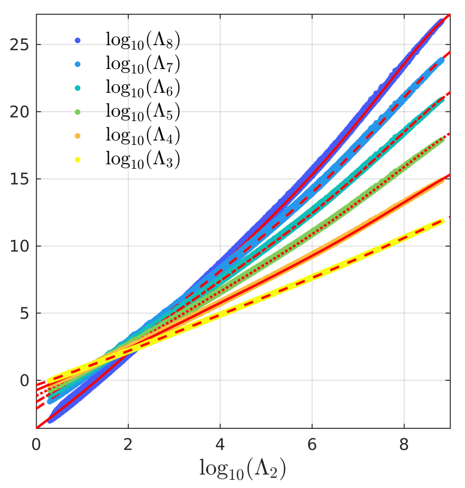
From our phenomenological EOS data set, we compute 21,994,104 valid individual NS solutions to the TOV equation as our statistics for analyzing the multipole Love relations. , , , , , and are plotted against in Figure 1, and one can appreciate the universality of each relation across a vast range of scales. (We observe that all the intersections between the six curves lie around , but we are not sure why this is the case.) As in the authors’ previous work [14], we employ a fitting function of the form
which is an extended version of the fitting function originally used by Yagi and Yunes [11]. The fitting parameters for each relation are given in Table 1.
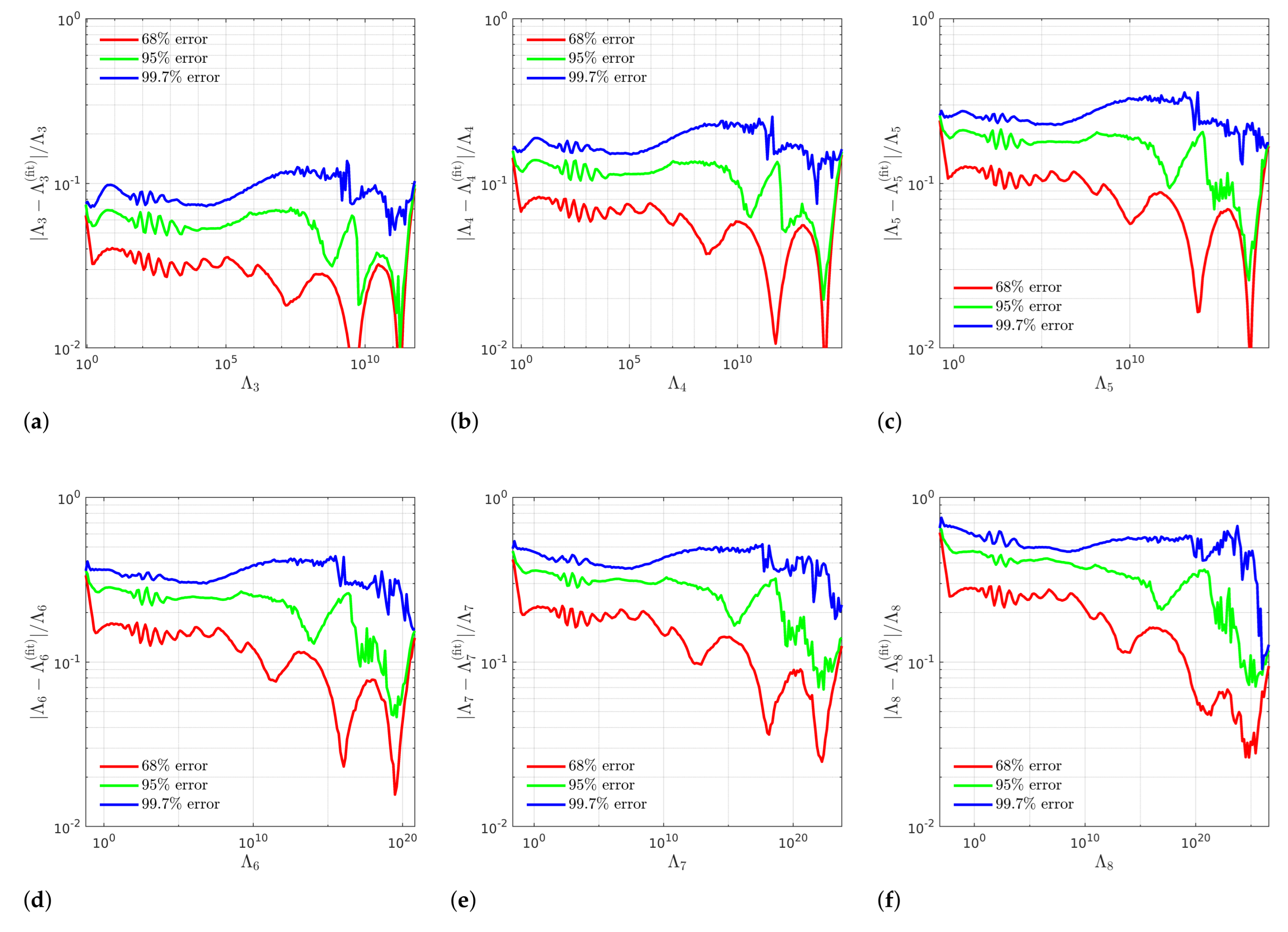
In Figure 2, we show the 68%, 95%, and 99.7% relative error of each fit. For each line in the error plot, the corresponding percentage of data points lie below it. We restrict our attention to the domain , as this is the range of most relevant to current LIGO measurements. The estimate error of each over this range stays mostly flat with a slight downward trend. (The small ripples that can be seen in the error plots over this range are simply artifacts of how the distribution of NS solutions was computed.) The universality of the multipole relations weaken gradually as l increases, as can be seen in the increasing thickness of the distributions in Figure 1. This then increases the maximum estimate error of for larger l despite the faithfulness of each fit to the shape of the corresponding relation (see Figure 1). While 95% of estimate errors are smaller than ∼7% for the – relation, 95% are only smaller than ∼50% for –.
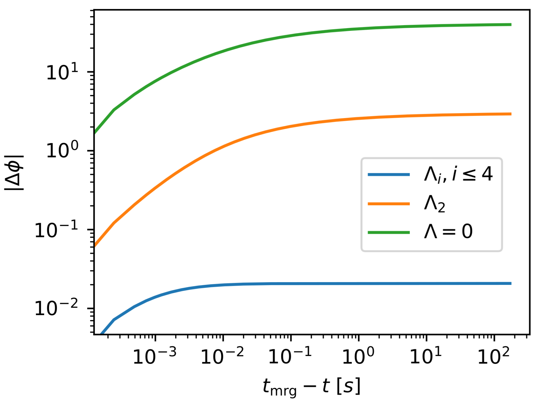
The phase of a GW in waveform modelling is affected by the highest order out to which one carries finite-size corrections (The leading-terms of the finite-size correction from is given in [12]). We demonstrate this with a baseline model of a binary with and using the spin-aligned effective-one-body waveform model TEOBResumS [18]. Often when universal relations are not employed, all finite-size effects are dropped except for the leading-order () effect. In the baseline model, just the correction alone contributes a phase difference of 36.7 radians compared to a waveform model with no tidal corrections. Further corrections from the and effects using the – and – relations, respectively, incur an additional 2.89 radians. Finally, including the , 6, 7, and 8 corrections using the relations given in this work adds 0.02 radians of dephasing on top of that. (The dephasing between the waveform model and models with fewer corrections is plotted in Figure 3 as a function of time. For all models, most of the dephasing is accumulated in the last 5 milliseconds before the merger.) Combined, the corrections contribute 2.91 radians of dephasing. This demonstrates the importance of the multipole Love relations for faithful waveform modelling.
The dephasing of the corrections are currently smaller than GW detector uncertainties, but this could only have been known after fitting to the multipole relations. Additionally, with the greater sensitivity of future detectors, the finite-size effects will start to come into view. The order out to which one should carry finite-size corrections in the waveform analysis of actual GW data is dependent on several factors (the EOS model, the signal-to-noise ratio of the merger, etc.); however, in general it is recommended that corrections up to be included in the analysis of data from current detectors [12,14,27].
4. - Relation
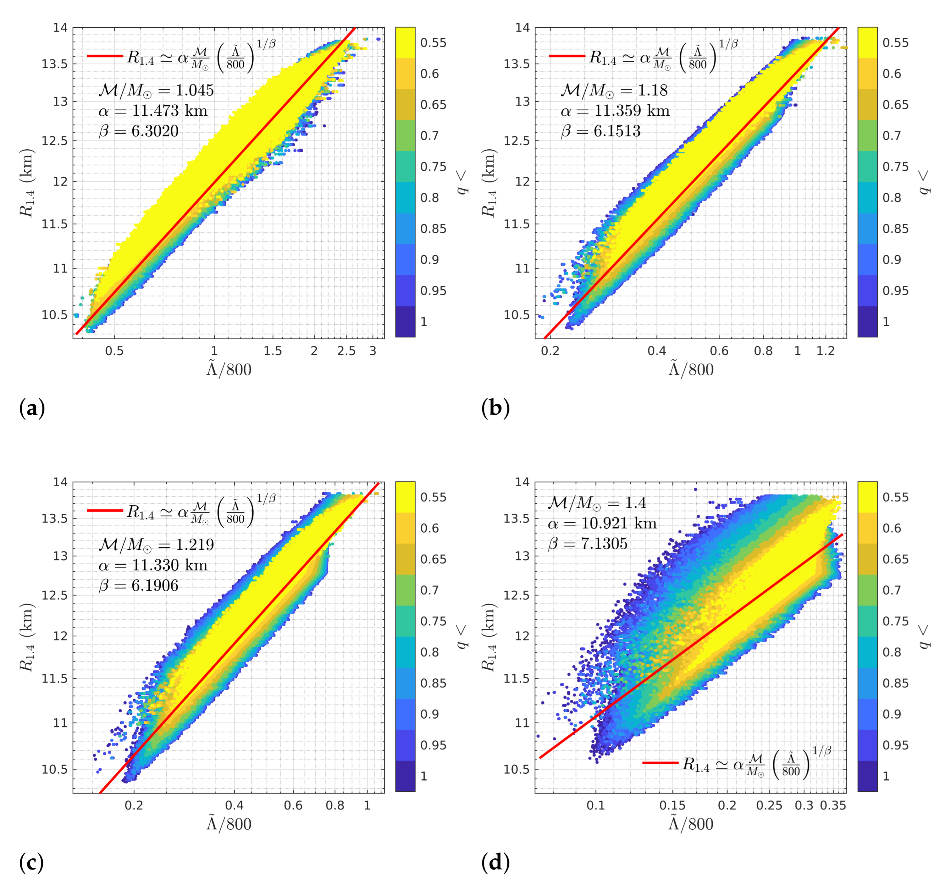
We analyze the - relation at twelve different fixed values of the chirp mass , which are given in Table 2. We compute between 750,000 and 1,000,000 valid individual binaries for each value of . Several example plots of the relation are shown in Figure 4. The relation’s dependence on the binary mass ratio q is illustrated by the coloring of the points in these plots. Each point in the plot represents a BNS. Points with smaller values of q are plotted on top. An important conclusion to draw from these plots is that the relation does not depend upon both stars having the same radius [19]. For , the relation remains fairly tight for all values of q. Further, for (The smallest physical value can take is when (see Section 2). Using Equation (3), this gives us . Since we permit and to be less than , we are able to reach as low as .), the relation actually becomes tighter as q decreases (i.e., as the radii of the two stars differ more and more), which can be understood by considering the definition of in Equation (2). For fixed , the range of possible values can take is constrained by q. When , the masses of the binary can span the range from the minimum to the maximum mass, . Hence, , and . As q decreases, the bounds for both and shrink and no longer overlap, causing the same to happen for and . This, as we see, also shrinks the bounds on . Thus, we expect the relation to tighten as q decreases.
We construct a fitting function for the - relation by considering a slightly generalized form of Equation (4):
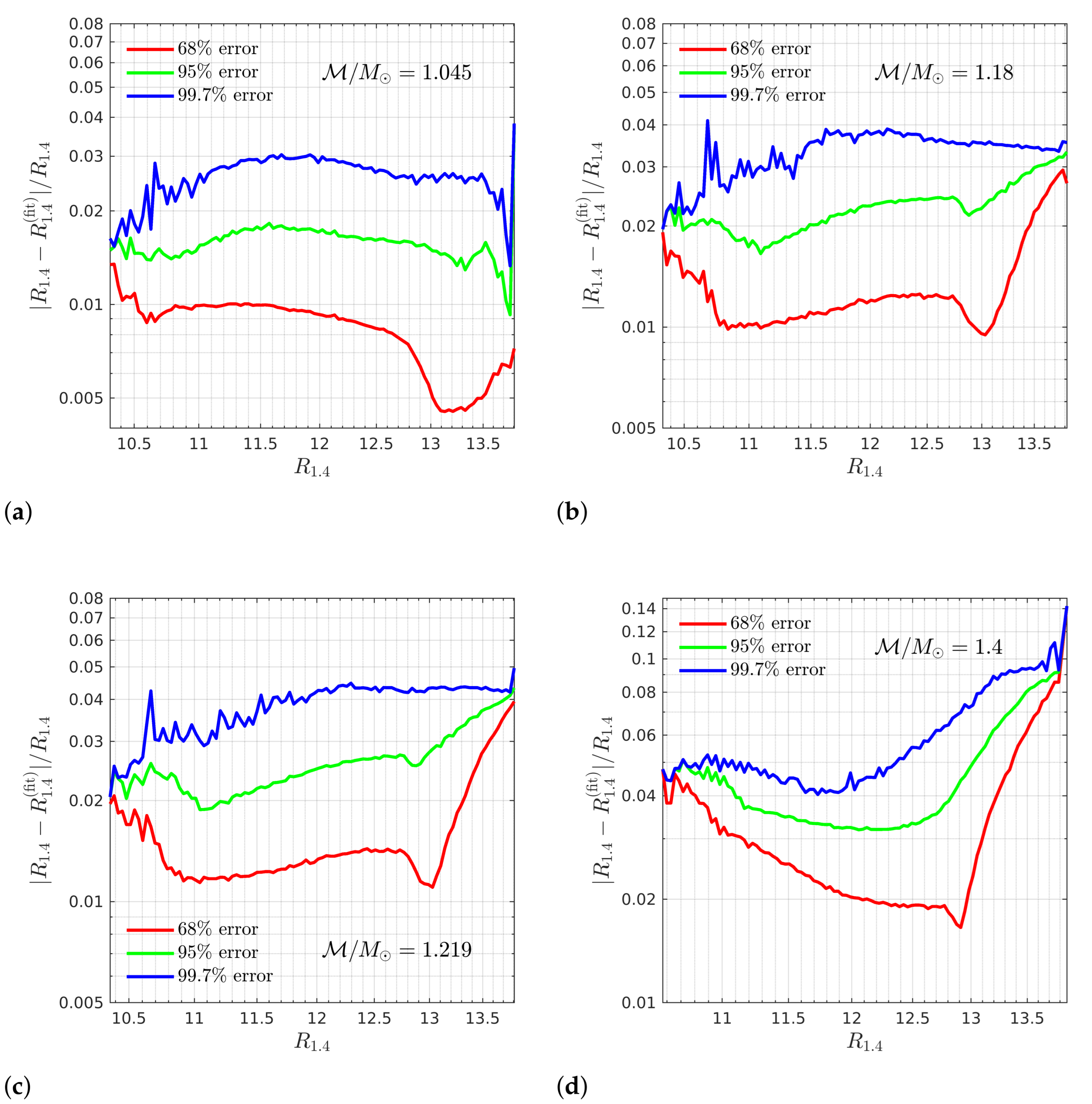
where, in this case, . Here the proportionality constant and the inverse exponent are the fitting parameters and, consequently, will be dependent on . These fits are also shown in Figure 4. The fitting parameters for all values of are given in Table 2. A sense of the accuracy of the estimated value of from the fit can be gathered from Figure 5, where we plot the 68%, 95%, and 99.7% relative error of the example fits. Overall, the estimates are accurate to within error for all values of , and are, in fact, accurate to within ∼5% for most values of .
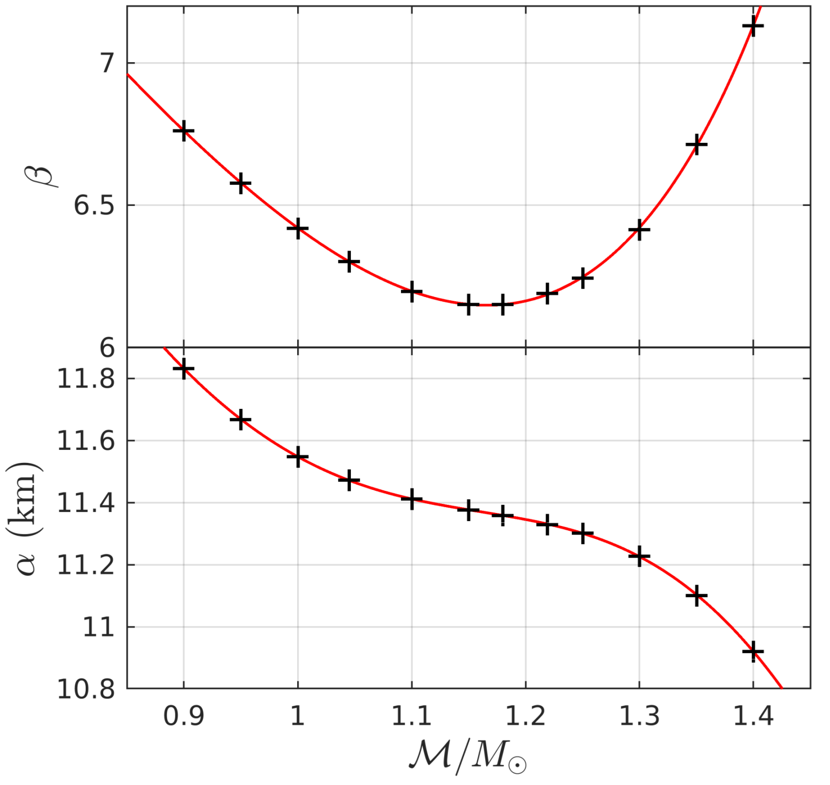
We can extend our fitting results to all by fitting the dependence of and on . We construct the rational fitting functions
where , , and . These fits, which are in excellent agreement the values in Table 2, are shown in Figure 6. The fitting parameters and for and are given in Table 3. What is interesting is that the inverse exponent is not monotonic. Rather, it has a minimum at . A possible contributor to this effect is the decrease in the variety of possible binaries as increases. The maximum value could take for a given EOS is found by letting in Equation (3), which yields . For , and are bounded by
Hence, as increases, the relation becomes gradually dominated by (1) EOSs with and (2) only those BNSs from each EOS that lie in the increasingly narrow range in Equation (9). This decrease of BNS variety could play a role in the non-monotonic behavior of .
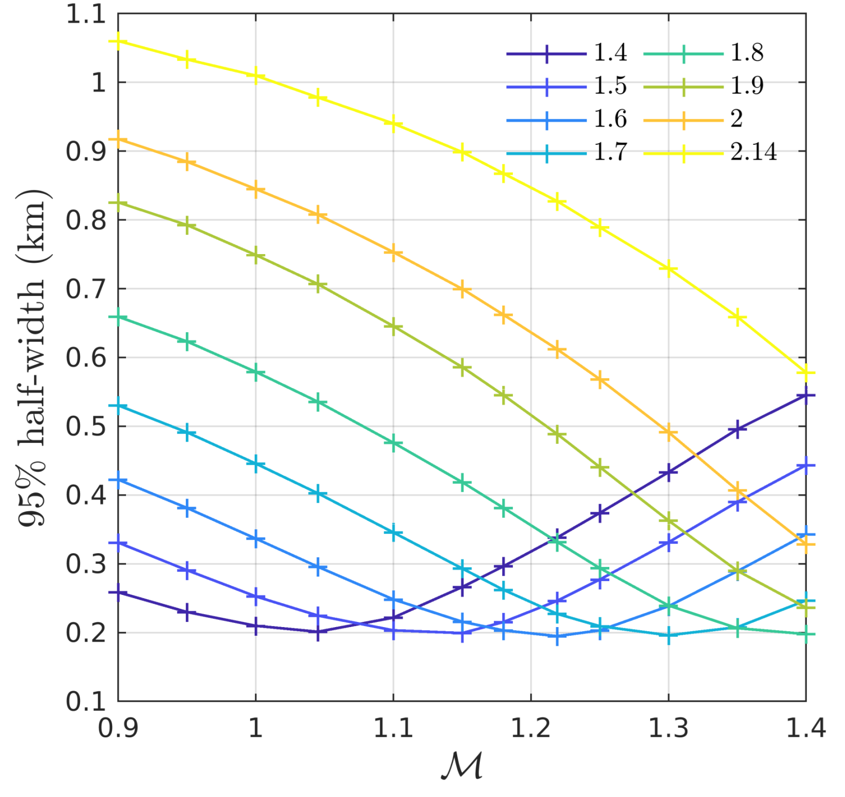
One could, of course, consider more generally the relation between and the radius of a NS with some mass M, . We pursue this thought by looking at – for , , , , , , 2, and . Just as for the - relation, we utilize the fitting function in Equation (4), and then find and as functions of x using Equation (8). In Table 3, we show the fitting parameters and of and for each M. The tightness of the – relation (and thus the general quality of the estimate from the fit) is dependent on both M and . We illustrate this in Figure 7 by plotting the approximate uncertainty of the estimated value of as a function of for several values of M. Since our EOSs and BNSs do not come from prior probability distributions, we non-stringently define the uncertainty here as the half-width of the symmetric interval centered at that encloses 95% of the data points in the histogram of for fixed . Interestingly, the uncertainty for each M reaches a minimum at some particular value of , with the minimum uncertainty for each M being around 0.2 km in the range of we considered. The minima for through are visible in Figure 7. This reveals that there is an optimal M for each such that is maximally constrained by the – relation at that . Thus, for example, a chirp mass of would yield the best estimate of , while a chirp mass of would yield the best estimate of . Further, there appears to be a linear dependence of the optimal M on ; however, a wider range of would need to be considered to confirm this. The change in the variety of BNSs as increases, as previously described, may contribute to this. At larger , the relation becomes dominated by larger mass NSs; thus, the relation may become more sensitive to the radii of larger mass NSs as increases.
The – relation, then, allows one to use any binary to place a robust, EOS-agnostic constraint on using just and . This offers great prospects for the upcoming LIGO O4 run and for third-generation detectors. The O4 run expects to see detections within a search volume of Mpc year [51]. Every BNS detection can be transformed into a maximum constrain on some . However, even the weaker constraints afforded by – are of still great utility. Just 10 weak constraints on using the - relation will yield a reliable value for . Further, a reduction in statistical uncertainty thanks to increased sensitivity improves the effectiveness of universal relations, as, for example, the systematic errors of fits to multipole relations are generally smaller than statistical uncertainty [12].
5. Conclusions
We supplement the tool set of GW analysis and waveform modelling by presenting entirely new fits to several universal relations between high-multipole-order dimensionless gravitoelectric tidal deformabilities and to the universal relation for BNS between the radius of the NS, , and the reduced tidal deformability . We compute these utilizing a data set of nearly two-million phenomenological EOS sampled from across a broad parameter space using an MCMC algorithm.
First, we present fits to the multipole relations. Previous fits [12,14] had been made to just the – and – relations. We extend the library of fits by looking at the –, –, –, and – relations. The tightness of the relations weakens as l increases. Consequently, though the fits are faithful to the shapes of the relations, the maximum estimate error of the fits increases to the order of 50% for . The inclusion of the finite-size effects of the multipoles in waveform analysis can incur as much as 0.02 radians of dephasing compared to including only the effects. Collectively, the effects contribute as much as 2.91 radians of dephasing, and it is recommended that finite-size corrections for multipoles be included in the analysis of GW data wherever they are at least comparable to detector uncertainties. The full usefulness of these relations in GW data analysis will be realized with the increased sensitivity of the upcoming third-generation GW detectors like LIGO III [22], the Einstein Telescope [23,24], and Cosmic Explorer [25], as the finite-size effects of these multipole orders are currently smaller than measurement error.
Next, we analyze the - relation. The original derivation of the relation [19] yields an expression, given in Equation (4), that is linearly dependent on the chirp mass of the BNS. Fitting the relation for different fixed values of reveals any nonlinear dependence the relation may have on and allows us to compute an expression that more accurately estimates . We do this for twelve different values of between and , using the fitting function in Equation (7). We then interpolate the fitting parameters to all by fitting them as functions of . The accuracy of the estimate of for any value of is found to be quite good. 95% of the estimates are within ∼5% of .
We then consider a generalized form of the relation – for a generic NS mass M. We perform the same analysis as for the - relation for seven other values of M. We find that the level of uncertainty in the estimate of depends on both M and . There is, in fact, an optimal value of M for each such that is maximally constrained by the relation at that value of . Therefore, this relation will be an excellent tool for combining the results from multiple GW detections of BNSs into constraints on NS radii.
The parameter space of possible EOS explored by our MCMC algorithm to compute our EOS data set can be further restricted with the inclusion of possible future LIGO/Virgo/KAGRA O4 constraints, laboratory constraints, such as those from heavy-ion collisions [52] and PREX [53], X-ray burst observations from NICER [54,55,56], and by combining the phenomenological EOSs with results from pQCD calculations [57].
Author Contributions
D.A.G. generated and analyzed the TOV data, D.A.G. and D.R. interpreted the results and wrote the manuscript. Both authors have read and agreed to the published version of the manuscript.
Funding
This research was funded by U.S. Department of Energy, Office of Science, Division of Nuclear Physics under Award Number(s) DE-SC0021177 and from the National Science Foundation under Grants No. PHY-2011725 and PHY-2116686. Computations for this research were performed on the Pennsylvania State University’s Institute for Computational and Data Sciences Advanced CyberInfrastructure (ICDS-ACI).
Data Availability Statement
EOS parameters and bulk properties of reference NSs generated for this work are publicly available on Zenodo [58].
Acknowledgments
The authors gratefully wish to acknowledge R. Gamba for waveform dephasing calculations and S. Bernuzzi for discussions that motivated us to start this work.
Conflicts of Interest
The authors declare no conflict of interest. The funders had no role in the design of the study; in the collection, analyses, or interpretation of data; in the writing of the manuscript, or in the decision to publish the results.
Abbreviations
The following abbreviations are used in this manuscript:
| EOS | Equation of state |
| NS | Neutron star |
| BNS | Binary neutron star |
| GW | Gravitational wave |
| MCMC | Markov chain Monte Carlo |
| TOV | Tolman-Oppenheimer-Volkoff |
References
- Andersson, N.; Kokkotas, K.D. Gravitational Waves and Pulsating Stars: What Can We Learn from Future Observations? Phys. Rev. Lett. 1996, 77, 4134–4137. [Google Scholar] [CrossRef] [PubMed] [Green Version]
- Andersson, N.; Kokkotas, K.D. Towards gravitational wave asteroseismology. Mon. Not. R. Astron. Soc. 1998, 299, 1059–1068. [Google Scholar] [CrossRef] [Green Version]
- Benhar, O.; Berti, E.; Ferrari, V. The imprint of the equation of state on the axial w-modes of oscillating neutron stars. Mon. Not. R. Astron. Soc. 1999, 310, 797–803. [Google Scholar] [CrossRef] [Green Version]
- Benhar, O.; Ferrari, V.; Gualtieri, L. Gravitational wave asteroseismology reexamined. Phys. Rev. D 2004, 70, 124015. [Google Scholar] [CrossRef]
- Tsui, L.K.; Leung, P.T. Universality in quasi-normal modes of neutron stars. Mon. Not. R. Astron. Soc. 2005, 357, 1029–1037. [Google Scholar] [CrossRef] [Green Version]
- Lau, H.K.; Leung, P.T.; Lin, L.M. Inferring Physical Parameters of Compact Stars from their f-mode Gravitational Wave Signals. Astrophys. J. 2010, 714, 1234–1238. [Google Scholar] [CrossRef] [Green Version]
- Bejger, M.; Haensel, P. Moments of inertia for neutron and strange stars: Limits derived for the Crab pulsar. Astron. Astrophys. 2002, 396, 917–921. [Google Scholar] [CrossRef] [Green Version]
- Lattimer, J.M.; Schutz, B.F. Constraining the Equation of State with Moment of Inertia Measurements. Astophys. J. 2005, 629, 979–984. [Google Scholar] [CrossRef] [Green Version]
- Urbanec, M.; Miller, J.C.; Stuchlík, Z. Quadrupole moments of rotating neutron stars and strange stars. Mon. Not. R. Astron. Soc. 2013, 433, 1903–1909. [Google Scholar] [CrossRef] [Green Version]
- Yagi, K.; Yunes, N. I-Love-Q: Unexpected Universal Relations for Neutron Stars and Quark Stars. Science 2013, 341, 365–368. [Google Scholar] [CrossRef] [Green Version]
- Yagi, K.; Yunes, N. I-Love-Q relations in neutron stars and their applications to astrophysics, gravitational waves, and fundamental physics. Phys. Rev. D 2013, 88, 023009. [Google Scholar] [CrossRef] [Green Version]
- Yagi, K. Multipole Love relations. Phys. Rev. D 2014, 89, 043011. [Google Scholar] [CrossRef] [Green Version]
- Yagi, K.; Stein, L.C.; Pappas, G.; Yunes, N.; Apostolatos, T.A. Why I-Love-Q: Explaining why universality emerges in compact objects. Phys. Rev. D 2014, 90, 063010. [Google Scholar] [CrossRef] [Green Version]
- Godzieba, D.A.; Gamba, R.; Radice, D.; Bernuzzi, S. Updated universal relations for tidal deformabilities of neutron stars from phenomenological equations of state. Phys. Rev. D 2021, 103, 063036. [Google Scholar] [CrossRef]
- Hinderer, T.; Lackey, B.D.; Lang, R.N.; Read, J.S. Tidal deformability of neutron stars with realistic equations of state and their gravitational wave signatures in binary inspiral. Phys. Rev. D 2010, 81, 123016. [Google Scholar] [CrossRef] [Green Version]
- Hinderer, T. Tidal Love Numbers of Neutron Stars. Astrophys. J. 2008, 677, 1216–1220. [Google Scholar] [CrossRef]
- Damour, T.; Nagar, A. Relativistic tidal properties of neutron stars. Phys. Rev. D 2009, 80, 084035. [Google Scholar] [CrossRef] [Green Version]
- Nagar, A.; Messina, F.; Rettegno, P.; Bini, D.; Damour, T.; Geralico, A.; Akcay, S.; Bernuzzi, S. Nonlinear-in-spin effects in effective-one-body waveform models of spin-aligned, inspiralling, neutron star binaries. Phys. Rev. D 2019, 99, 044007. [Google Scholar] [CrossRef] [Green Version]
- Zhao, T.; Lattimer, J.M. Tidal deformabilities and neutron star mergers. Phys. Rev. D 2018, 98, 063020. [Google Scholar] [CrossRef] [Green Version]
- Yagi, K.; Yunes, N. Approximate universal relations for neutron stars and quark stars. Phys. Rep. 2017, 681, 1–72. [Google Scholar] [CrossRef] [Green Version]
- Gamba, R.; Breschi, M.; Bernuzzi, S.; Agathos, M.; Nagar, A. Waveform systematics in the gravitational-wave inference of tidal parameters and equation of state from binary neutron star signals. arXiv 2020, arXiv:2009.08467. [Google Scholar]
- Adhikari, R.X. Gravitational radiation detection with laser interferometry. Rev. Mod. Phys. 2014, 86, 121–151. [Google Scholar] [CrossRef]
- Einstein Telescope. Available online: http://www.et-gw.eu/ (accessed on 29 September 2021).
- Hild, S.; Chelkowski, S.; Freise, A. Pushing towards the ET sensitivity using ’conventional’ technology. arXiv 2008, arXiv:0810.0604. [Google Scholar]
- Reitze, D.; Adhikari, R.X.; Ballmer, S.; Barish, B.; Barsotti, L.; Billingsley, G.; Brown, D.A.; Chen, Y.; Coyne, D.; Eisenstein, R.; et al. Contribution to Gravitational-Wave Astronomy beyond LIGO. Bull. Am. Astron. Soc. 2019, 51, 35. [Google Scholar]
- Flanagan, É.É.; Hinderer, T. Constraining neutron-star tidal Love numbers with gravitational-wave detectors. Phys. Rev. D 2008, 77, 021502. [Google Scholar] [CrossRef] [Green Version]
- Damour, T.; Nagar, A.; Villain, L. Measurability of the tidal polarizability of neutron stars in late-inspiral gravitational-wave signals. Phys. Rev. D 2012, 85, 123007. [Google Scholar] [CrossRef] [Green Version]
- De, S.; Finstad, D.; Lattimer, J.M.; Brown, D.A.; Berger, E.; Biwer, C.M. Tidal Deformabilities and Radii of Neutron Stars from the Observation of GW170817. Phys. Rev. Lett. 2018, 121, 091102. [Google Scholar] [CrossRef] [Green Version]
- Postnikov, S.; Prakash, M.; Lattimer, J.M. Tidal Love numbers of neutron and self-bound quark stars. Phys. Rev. D 2010, 82, 024016. [Google Scholar] [CrossRef] [Green Version]
- Yagi, K.; Yunes, N. Binary Love relations. Class. Quantum Gravity 2016, 33, 13LT01. [Google Scholar] [CrossRef] [Green Version]
- Maselli, A.; Cardoso, V.; Ferrari, V.; Gualtieri, L.; Pani, P. Equation-of-state-independent relations in neutron stars. Phys. Rev. D 2013, 88, 023007. [Google Scholar] [CrossRef] [Green Version]
- Abbott, B. GW170817: Observation of Gravitational Waves from a Binary Neutron Star Inspiral. Phys. Rev. Lett. 2017, 119, 161101. [Google Scholar] [CrossRef] [Green Version]
- Abbott, B. GW170817: Measurements of Neutron Star Radii and Equation of State. Phys. Rev. Lett. 2018, 121, 161101. [Google Scholar] [CrossRef] [Green Version]
- Essick, R.; Landry, P.; Holz, D.E. Nonparametric inference of neutron star composition, equation of state, and maximum mass with GW170817. Phys. Rev. D 2020, 101, 063007. [Google Scholar] [CrossRef] [Green Version]
- Read, J.S.; Lackey, B.D.; Owen, B.J.; Friedman, J.L. Constraints on a phenomenologically parametrized neutron-star equation of state. Phys. Rev. D 2009, 79, 124032. [Google Scholar] [CrossRef] [Green Version]
- Bernuzzi, S.; Nagar, A. Gravitational waves from pulsations of neutron stars described by realistic Equations of State. Phys. Rev. 2008, D78, 024024. [Google Scholar] [CrossRef] [Green Version]
- Demorest, P.; Pennucci, T.; Ransom, S.; Roberts, M.; Hessels, J. Shapiro Delay Measurement of A Two Solar Mass Neutron Star. Nature 2010, 467, 1081–1083. [Google Scholar] [CrossRef]
- Fonseca, E. The NANOGrav Nine-year Data Set: Mass and Geometric Measurements of Binary Millisecond Pulsars. Astrophys. J. 2016, 832, 167. [Google Scholar] [CrossRef]
- Arzoumanian, Z. The NANOGrav 11-year Data Set: High-precision timing of 45 Millisecond Pulsars. Astrophys. J. Suppl. 2018, 235, 37. [Google Scholar] [CrossRef] [Green Version]
- Antoniadis, J. A Massive Pulsar in a Compact Relativistic Binary. Science 2013, 340, 6131. [Google Scholar] [CrossRef] [PubMed] [Green Version]
- Cromartie, H.T. Relativistic Shapiro delay measurements of an extremely massive millisecond pulsar. Nat. Astron. 2019, 4, 72–76. [Google Scholar] [CrossRef] [Green Version]
- Linares, M.; Shahbaz, T.; Casares, J. Peering into the dark side: Magnesium lines establish a massive neutron star in PSR J2215+5135. Astrophys. J. 2018, 859, 54. [Google Scholar] [CrossRef]
- Margalit, B.; Metzger, B.D. Constraining the Maximum Mass of Neutron Stars From Multi-Messenger Observations of GW170817. Astrophys. J. Lett. 2017, 850, L19. [Google Scholar] [CrossRef]
- Shibata, M.; Fujibayashi, S.; Hotokezaka, K.; Kiuchi, K.; Kyutoku, K.; Sekiguchi, Y.; Tanaka, M. Modeling GW170817 based on numerical relativity and its implications. Phys. Rev. 2017, D96, 123012. [Google Scholar] [CrossRef] [Green Version]
- Rezzolla, L.; Most, E.R.; Weih, L.R. Using gravitational-wave observations and quasi-universal relations to constrain the maximum mass of neutron stars. Astrophys. J. Lett. 2018, 852, L25. [Google Scholar] [CrossRef]
- Ruiz, M.; Shapiro, S.L.; Tsokaros, A. GW170817, General Relativistic Magnetohydrodynamic Simulations, and the Neutron Star Maximum Mass. Phys. Rev. 2018, D97, 021501. [Google Scholar] [CrossRef] [Green Version]
- Shibata, M.; Zhou, E.; Kiuchi, K.; Fujibayashi, S. Constraint on the maximum mass of neutron stars using GW170817 event. Phys. Rev. 2019, D100, 023015. [Google Scholar] [CrossRef] [Green Version]
- Godzieba, D.A.; Radice, D.; Bernuzzi, S. On the Maximum Mass of Neutron Stars and GW190814. Astrophys. J. 2021, 908, 122. [Google Scholar] [CrossRef]
- Martinez, J.G.; Stovall, K.; Freire, P.C.C.; Deneva, J.S.; Jenet, F.A.; McLaughlin, M.A.; Bagchi, M.; Bates, S.D.; Ridolfi, A. Pulsar J0453+1559: A Double Neutron Star System with a Large Mass Asymmetry. Astrophys. J. 2015, 812, 143. [Google Scholar] [CrossRef] [Green Version]
- Suwa, Y.; Yoshida, T.; Shibata, M.; Umeda, H.; Takahashi, K. On the minimum mass of neutron stars. Mon. Not. R. Astron. Soc. 2018, 481, 3305–3312. [Google Scholar] [CrossRef] [Green Version]
- Abbott, B.P. Prospects for observing and localizing gravitational-wave transients with Advanced LIGO, Advanced Virgo and KAGRA. Living Rev. Relativ. 2020, 23, 3. [Google Scholar] [CrossRef]
- Danielewicz, P.; Lacey, R.; Lynch, W.G. Determination of the Equation of State of Dense Matter. Science 2002, 298, 1592–1596. [Google Scholar] [CrossRef] [Green Version]
- Reed, B.T.; Fattoyev, F.J.; Horowitz, C.J.; Piekarewicz, J. Implications of PREX-2 on the Equation of State of Neutron-Rich Matter. Phys. Rev. Lett. 2021, 126, 172503. [Google Scholar] [CrossRef]
- Steiner, A.W.; Lattimer, J.M.; Brown, E.F. The Equation of State from Observed Masses and Radii of Neutron Stars. Astrophys. J. 2010, 722, 33–54. [Google Scholar] [CrossRef]
- Lattimer, J.M. The Nuclear Equation of State and Neutron Star Masses. Annu. Rev. Nucl. Part. Sci. 2012, 62, 485–515. [Google Scholar] [CrossRef] [Green Version]
- Özel, F.; Freire, P. Masses, Radii, and the Equation of State of Neutron Stars. Ann. Rev. Astro. Astrophys. 2016, 54, 401–440. [Google Scholar] [CrossRef] [Green Version]
- Annala, E.; Gorda, T.; Kurkela, A.; Nättilä, J.; Vuorinen, A. Evidence for quark-matter cores in massive neutron stars. Nat. Phys. 2020, 16, 907–910. [Google Scholar] [CrossRef]
- Godzieba, D.A.; Radice, D.; Bernuzzi, S. Phenomenological EOS Data Set. Zenodo 2020. [Google Scholar] [CrossRef]
Figure 1.
Universal multipole Love relations for through from the collection of phenomenological EOSs. We use the fitting function function in Equation (6), and the fit to each relation is plotted in red.
Figure 1.
Universal multipole Love relations for through from the collection of phenomenological EOSs. We use the fitting function function in Equation (6), and the fit to each relation is plotted in red.

Figure 2.
68%, 95%, and 99.7% relative errors of the fits to (a) –, (b) –, (c) –, (d) –, (e) –, and (f) – relations. The small ripple in the error seen at small values of each is simply an artifact of how the distribution of NS solutions were generated. The fits are faithful to the shape of the curves of the relations; however, universality weakens and the distributions of points spread out as l increases, resulting in the maximum error of the estimate increasing with l.

Figure 3.
An example of dephasing between different waveform models (one with no tides, one with only the correction, and one with all corrections up to ) and the full model (all corrections up to ). The overall dephasing is very small between the model and the full model. Most of the dephasing is accumulated in the last 5 milliseconds, just a few orbits prior to the merger.

Figure 4.
Example fits to the - relation for (a) , (b) , (c) , and (d) . Each point represents a BNS and is colored according to the value of the binary mass ratio . Points with smaller values of q are drawn on top. The upper limit on the value of for each derives from the cutoff for the NS imposed on the EOSs generated by our algorithm (see Section 2). The relation does not depend on both NSs having the same radius, and indeed for it becomes tighter as q decreases.

Figure 5.
68%, 95%, and 99.7% relative errors of the fits to the - relation for (a) , (b) , (c) , and (d) . The error overall stays below , with 95% of the estimates generally below 4–5% error, for all values of .
Figure 5.
68%, 95%, and 99.7% relative errors of the fits to the - relation for (a) , (b) , (c) , and (d) . The error overall stays below , with 95% of the estimates generally below 4–5% error, for all values of .

Figure 6.
Fitting parameters and of the - relation as functions of . does not vary monotonically with x, but has a minimum.
Figure 6.
Fitting parameters and of the - relation as functions of . does not vary monotonically with x, but has a minimum.

Figure 7.
The approximate uncertainty of the estimated value of computed using the – relation as a function of . Each curve is colored according to the value of M (given in units of ). The uncertainty is defined as the half-width of the symmetric interval centered at that encloses 95% of the data points in the histogram of . For every M, there is an optimal value of such that this uncertainty is minimized.


Table 1.
Fitting parameters of the multipole Love relations given in Equation (6).
Table 1.
Fitting parameters of the multipole Love relations given in Equation (6).
| Relation | |||||||
|---|---|---|---|---|---|---|---|
| – | |||||||
| – | |||||||
| – | |||||||
| – | |||||||
| – | |||||||
| – |
Table 2.
Fitting parameters of the general - relation given in Equation (7) for different values of .
Table 2.
Fitting parameters of the general - relation given in Equation (7) for different values of .
| (km) | ||
|---|---|---|
| 0.900 | 11.832 | 6.7621 |
| 0.950 | 11.668 | 6.5775 |
| 1.000 | 11.548 | 6.4189 |
| 1.045 | 11.473 | 6.3020 |
| 1.100 | 11.412 | 6.1972 |
| 1.150 | 11.377 | 6.1515 |
| 1.180 | 11.359 | 6.1513 |
| 1.219 | 11.330 | 6.1906 |
| 1.250 | 11.302 | 6.2441 |
| 1.300 | 11.228 | 6.4147 |
| 1.350 | 11.102 | 6.7139 |
| 1.400 | 10.921 | 7.1305 |
Table 3.
Fitting parameters and for and as functions of , where and for several values of M. The fitting functions are given in Equation (3).
Table 3.
Fitting parameters and for and as functions of , where and for several values of M. The fitting functions are given in Equation (3).
| 1.4 | - | 1 | ||||||
| 1 | ||||||||
| 1.5 | - | 1 | ||||||
| 1 | ||||||||
| 1.6 | - | 1 | ||||||
| 1 | ||||||||
| 1.7 | - | 1 | ||||||
| 1 | ||||||||
| 1.8 | - | 1 | ||||||
| 1 | ||||||||
| 1.9 | - | 1 | ||||||
| 1 | ||||||||
| 2 | 63,061 | - | 1 | |||||
| 1 | ||||||||
| 2.14 | 93,209 | - | 12,686 | 1 | ||||
| 58,353 | 1 |
Publisher’s Note: MDPI stays neutral with regard to jurisdictional claims in published maps and institutional affiliations. |
© 2021 by the authors. Licensee MDPI, Basel, Switzerland. This article is an open access article distributed under the terms and conditions of the Creative Commons Attribution (CC BY) license (https://creativecommons.org/licenses/by/4.0/).
Share and Cite
MDPI and ACS Style
Godzieba, D.A.; Radice, D. High-Order Multipole and Binary Love Number Universal Relations. Universe 2021, 7, 368. https://0-doi-org.brum.beds.ac.uk/10.3390/universe7100368
AMA Style
Godzieba DA, Radice D. High-Order Multipole and Binary Love Number Universal Relations. Universe. 2021; 7(10):368. https://0-doi-org.brum.beds.ac.uk/10.3390/universe7100368
Chicago/Turabian StyleGodzieba, Daniel A., and David Radice. 2021. "High-Order Multipole and Binary Love Number Universal Relations" Universe 7, no. 10: 368. https://0-doi-org.brum.beds.ac.uk/10.3390/universe7100368
Note that from the first issue of 2016, this journal uses article numbers instead of page numbers. See further details here.