
Almost-Pseudo-Ricci Symmetric FRW Universe with a Dynamic Cosmological Term and Equation of State


1
Department of Mathematics, Birla Institute of Technology and Science-Pilani, Hyderabad Campus, Hyderabad 500078, India
2
Department of Mathematical and Actuarial Sciences, Universiti Tunku Abdul Rahman, Jalan Sungai Long, Cheras 43000, Malaysia
3
Institute of Mathematical Sciences, University of Malaya, Kuala Lumpur 50603, Malaysia
*
Author to whom correspondence should be addressed.
Universe 2021, 7(7), 205; https://0-doi-org.brum.beds.ac.uk/10.3390/universe7070205
Submission received: 15 May 2021
/
Revised: 6 June 2021
/
Accepted: 9 June 2021
/
Published: 22 June 2021
(This article belongs to the Special Issue Cosmological Tests of Theories of Gravity)
Abstract
:The objective of the present paper is to investigate an almost-pseudo-Ricci symmetric FRW spacetime with a constant Ricci scalar in a dynamic cosmological term and equation of state (EoS) scenario. Several cosmological parameters are calculated in this setting and thoroughly studied, which shows that the model satisfies the late-time accelerating expansion of the universe. We also examine all of the energy conditions to check our model’s self-stability.
1. Introduction
Ricci calculus in semi-Riemannian manifolds has a very rich history in the literature, which might have started from the concept of local symmetry, where the curvature tensor is parallel in the sense that , and later extended to conformally symmetric manifolds [1], recurrent manifolds [2], conformally recurrent manifolds [3], pseudo-symmetric manifolds [4], weakly symmetric manifolds [5], weakly Ricci symmetric manifolds [6], pseudo-Ricci symmetric manifolds [7], etc., as well as their interactions with general relativity. It should be noted that the standard theory of gravity governed by Einstein’s field equations (EFEs), which were introduced in 1915, is a very complicated system of partial differential equations and that different types of symmetries are commonly used to find the exact solutions; these kinds of restrictions on Riemannian or Ricci curvature tensors or on their covariant derivatives are very popular for such uses. In the present paper, we will consider an almost-pseudo-Ricci symmetric manifold , which was defined by Chaki and Kawaguchi [8] as a non-flat semi-Riemannian manifold whose Ricci curvature tensor is not identically zero and satisfies the condition
where and are the associated covariant tensors. The geometrical aspects of can be found in [9,10] and the references therein. This concept was introduced as a more generalized version of the pseudo-Ricci symmetric manifold [7], which is defined as a non-flat semi-Riemannian manifold whose Ricci curvature tensor is not identically zero and satisfies the condition
While studying curvature restrictions on a certain kind of conformally flat space of class one, the authors [11] obtained the expression of the covariant derivative of the Ricci curvature, which motivated the introduction of the . When in (1), reduces to . A vital result in is that if its Ricci scalar is constant, then it is considered Ricci scalar flat [7].
If the Ricci tensor of a Lorentzian manifold satisfies (1), then it is said to be an almost-pseudo-Ricci symmetric spacetime. In [9], the authors proved the existence of a conformally flat with a non-zero and non-constant Ricci scalar with a non-trivial example. Some geometric properties of were studied in [10], and a sufficient condition for such a spacetime to be perfect fluid was obtained; a conformally flat case was also briefly considered, and non-trivial examples were constructed. A perfect fluid spacetime solution of Einstein’s field equations without a cosmological constant was investigated in [12]. The authors of [13] showed that a conformally flat reduced to a Robertson–Walker spacetime, and in Einstein’s field equations with a cosmological constant, the stress–energy tensor was a perfect fluid with non-constant pressure and energy density when the underlying metric was . spacetimes were very recently studied with respect to modified gravity theories in [14]. It was shown that under certain conditions that were imposed on its scale factor, a Robertson–Walker spacetime was and vice-versa. Investigations of various energy conditions were carried out in some popular models of -gravity in spacetime.
The original field equations of general relativity introduced in 1915 by Einstein were amended by him after a couple of years in order to abolish the provision of a non-static universe in his theory by introducing the so-called cosmological constant . Einstein’s field equations with the cosmological constant are expressed as
where R is the trace of the Ricci curvature tensor and is the stress–energy tensor describing the matter content, which is assumed to be a perfect fluid and is given by , where and p are the energy density and the isotropic pressure, respectively, and the timelike is the velocity vector field of the fluid.
Moreover, at one point in the history of cosmological research, the cosmological constant turned into “the greatest blunder," which was pointed out by Einstein after the emergence of observational evidence of an expanding universe in the 1930s. Several studies were performed to explain this late-time inflation, but without any concrete conclusions. More recently, the present generation of cosmologists proposed the existence of an as-yet undetected dark energy (DE) that drives the evolution of the late-time universe, and the cosmological constant regained the limelight as the simplest contributing factor of the DE. However, currently, cosmologists believe that the accelerated expansion of the universe is driven by the unknown form of energy called “dark energy”, but the actual properties of dark energy are still unknown to us. The cosmological constant is the only candidate on the fundamental level of gravity that describes the accelerated expansion of the universe—i.e., in GR—as an alternative to dark energy. Moreover, “What is the value of the cosmological constant?” is a long-debatable question. Nevertheless, if string theory is the ultimate quantum gravity theory, then according to the second of the swampland conjectures, there is evidence that exact de Sitter solutions with a positive cosmological constant cannot account for the fate of the late-time universe [15,16]. Therefore, the above arguments motivate us to study the cosmological models with a time-dependent cosmological constant. Therefore, so-called constant is now considered as a time-varying dynamic variable in order to remove some fundamental problems that it has faced as the central character of DE. There are innumerable dynamic models in the literature; one of the oldest and most popular is the model , which was introduced by Carvalho et al. [17] and Waga [18]. In addition, Z. Yousaf investigated some interesting cosmological models based on [19,20]. In addition, p and in the stress–energy tensor are assumed to be related by an equation of state of the form . However, the choice of the constant EoS parameter is too restrictive [21], and thus, amongst a variety of possibilities, researchers considered linear and periodic functional forms of the EoS as alternatives [22,23,24].
The present paper is organized as follows: In Section 2, we construct the cosmological model and calculate the Hubble parameters (H). In Section 3, we discuss the cosmological parameters, such as the Hubble (H), deceleration (q), jerk (j), snap (s), and lerk (l) parameters, and present their profiles for two different cases of time-varying EoS models. In Section 4, we examine the energy conditions to check the self-consistency of our models. Finally, we discuss our results in Section 5.
2. The Field Equations
In an , the covariant derivative of the Ricci tensor satisfies (1). Hence, we have
which, on contraction over j and k, gives us
Again, the trace of (3) gives
Combining these, we conclude that
Using the EoS parameter , (8) gives
In an FRW spacetime with a decay law , the above equation ultimately gives us
Now, one can explore the evolution of the cosmological models by fixing the forms of , calculating the Hubble parameter from (10), and continuing from there.
3. Cosmological Parameters
Cosmological parameters, such as the Hubble, deceleration, jerk, snap, and lerk parameters, are the coefficients in the Taylor series expansion of the scale factor , i.e., the derivatives of . The study of these parameters gives us more insight into the evolution of the universe, and it also helps us compare theoretical measurements to existing observational values. Moreover, many investigations have been performed on cosmological parameters, such as by Mandal et al., who studied the accelerated expansion of the universe by presuming special deceleration parameters that evolved in all phases of the universe [25], used them to check the self-stability of cosmological models that focused on the present scenario of the universe [26], used them to constrain the Lagrangian function with the latest Pantheon data [27], and so on. The Taylor series expansion of the scale factor up to its fifth order can be written as
Here, the coefficients are nothing but the cosmological parameters, and the subscript “0” indicates the values of the parameters for the present time. represent the Hubble, deceleration, jerk, snap, and lerk parameters, respectively. These parameters are given by
The Hubble parameter and deceleration parameter , which are constrained by observations, predict the rate of expansion and the evolution of the universe (i.e., different phases of the universe), respectively. The jerk parameter explains the deceleration parameter’s evolution and predicts the future. Furthermore, the other two parameters, the snap and lerk, give helpful directions for the emergence of sudden future singularities [28].
3.1. Model 1:
To proceed further, we presume an equation-of-state parameter that is dependent on the cosmic time t [22]:
where and b are arbitrary constants. Using this in (10), we calculate the Hubble parameter as
where
and km/s/Mpc [29].
Using Equation (13), we can write the deceleration parameter as follows:
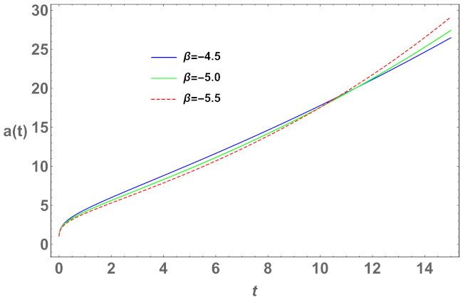
The evolution profile of the scale factor is depicted in Figure 1 by using software due to the complex expression of H. It evolves with cosmic time. From Figure 2, it is observed that the Hubble parameter decreases as time goes on. This result shows that the universe is presently expanding at a speed that is nearly identical from time to time. The profile of the deceleration parameter is presented in Figure 3. One can see that it evolves from a deceleration phase to an acceleration phase. The jerk, lerk, and snap parameters’ behaviours are shown in Figure 4. The jerk and lerk parameters decrease as time goes on and lie in their positive range, while the snap parameter is an increasing function and completely lies in its negative range, as shown in Figure 4.
3.2. Model 2:
In this subsection, we consider an equation-of-state parameter that is dependent on a trigonometric function [22], which is presented in Equation (15).
where and k are arbitrary constants.
Then, we calculate the following expression for the Hubble parameter:
Furthermore, we can write the deceleration parameter for the second model as
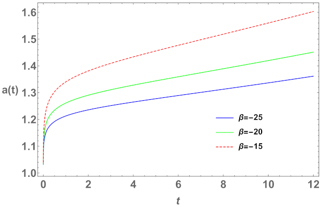
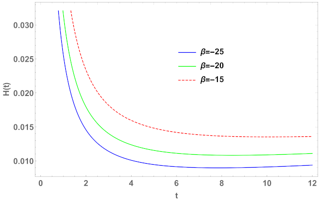
The evolution profile of the scale factor is depicted in Figure 5. One can see that it evolves with cosmic time. The profile of the Hubble parameter is presented in Figure 6 for different values of with respect to cosmic time t. One can see that the expansion rate in the early stage of the universe was very high in comparison to the present stage. Figure 7 presents the evolution of the deceleration parameter for the second model. It suggests that the evolution of the universe started from the deceleration phase and went through an accelerated phase. In addition, the profiles of the jerk, snap, and lerk parameters are shown in Figure 8. Furthermore, these profiles are in agreement with the current status of the universe.
4. Self-Stability Analysis of the Cosmological Model
Energy conditions are some of the greatest tools for examining cosmological models’ self-stability, and they are generally derived from the well-known Raychaudhuri equation [30]. They also help us describe the spacetime curve’s geometrical behaviour—including spacelike, timelike, or lightlike behaviour—and gives new insights into dreadful singularities [31]. They can be defined as:
- Strong energy conditions (SEC): ;
- Weak energy conditions (WEC): ;
- Null energy conditions (NEC): ;
- Dominant energy conditions (DEC): .
For the first model, we can write the expressions for energy density and pressure p as follows:
Using (18) and (19), we present all energy conditions’ profiles in Figure 9 for first model. It is observed that the SEC and WEC were violated while the others were satisfied. These results are analogous to those of scalar–tensor gravity models [32].
For the second model, we can write the expressions for energy density and pressure p as follows:
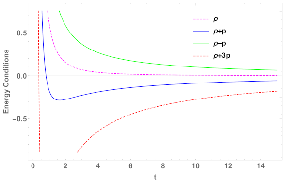
The profiles of all energy conditions are depicted in Figure 10, for second model. It is worth noting that our second model’s results are aligned with those of the first model in late time, i.e., both models represent the late-time accelerated expansion of the universe. In addition, if we compare our results with the existing results in the literature, such as the energy conditions in modified gravity found by K. Bamba et al. [33], then the main advantage of our models is that we explored all of the , while they focused only on the WEC and NEC. Nevertheless, we have presented our models with a concentration on the present observational evidence of the universe.
5. Discussion
In this manuscript, we studied an almost-pseudo-Ricci symmetric FRW universe. A cosmological model was constructed using the dynamical system method in the presence of . Among the different parametrizations of the term, the most popular is to express it through the cosmic scale factor a or the Hubble parameter H. Here, we considered the ansatz . Recent observational datasets suggest that our universe is going through an accelerated expansion phase, and its cause is an unknown form of energy called “dark energy’. Furthermore, is the simplest candidate for dark energy and the exploration of the present interest.
In this work, we calculated the Hubble parameter (H) by considering a particular case for dynamic and two different cases for a time-varying EoS . In the first model, we analyzed the cosmological model by taking the EoS parameter as a linear function of t; for the second case, we took it as a periodic or, more precisely, a cosine function. The profiles of H are presented in Figure 2 and Figure 6 for three different values of the model parameter for both cases. One can see that H decreases as time goes on, which shows that the expansion rate reduces from time to time. The deceleration parameter’s behaviours are shown in Figure 3 and Figure 7. Interestingly, our setting shows that the universe evolved from a decelerated phase to an accelerated phase. In addition, the jerk, snap, and lerk parameters’ profiles are depicted in Figure 4 and Figure 8. These profiles are compatible with the accelerated expansion of the universe. This is due to the modification of the original theory of gravity (i.e., in the presence of ).
As is known, energy conditions are used to describe the causal and geodesic structure of spacetime and to check the self-consistency of cosmological models. Therefore, to check our model’s self-stability, we tested all of the energy conditions and presented them in Figure 9 and Figure 10. We observed that the energy density is always positive throughout the evolution. It is interesting to note here that the SEC and WEC were violated, while the other energy conditions were satisfied. These results are also compatible with the present scenario of the universe and align with the results of scalar–tensor gravity models [32] and modified gravity theories (such as Horndeski theories [34,35] and gravity theory [26]). We hope that this study sheds some light on the present scenario of the universe. In addition, in the future, it will be interesting to study the almost-pseudo-Ricci symmetric FRW universe with a more generalized form of .
Author Contributions
S.M.: Writing–Original draft preparation, Investigation, Graph plotting, A.D.: Writing–Original draft preparation, Methodology, Formal analysis, Conceptualization, T.-H.L.: Methodology, Formal analysis, Conceptualization, P.K.S.: Writing–Reviewing and Editing, Validation, Project administration. All authors have read and agreed to the published version of the manuscript.
Funding
This research received no external funding.
Institutional Review Board Statement
Not applicable.
Informed Consent Statement
Not applicable.
Data Availability Statement
No data used in this article.
Acknowledgments
A.D. and T.-H.L. were supported by the grant FRGS/1/2019/STG06/UM/02/6. S.M. acknowledges the Department of Science and Technology (DST), Govt. of India, New Delhi for awarding a Junior Research Fellowship (File No. DST/INSPIRE Fellowship/2018/IF180676).
Conflicts of Interest
The authors declare no conflict of interest.
References
- Chaki, M.C.; Gupta, B. On conformally symmetric spaces. Indian J. Math. 1963, 5, 113–295. [Google Scholar]
- Walker, A.G. On Ruse’s space of recurrent curvature. Proc. Lond. Math. Soc. 1950, 52, 36–54. [Google Scholar] [CrossRef]
- Adati, T.; Miyazawa, T. On a Riemannian space with recurrent conformal curvatur. Tensor 1967, 18, 348–354. [Google Scholar]
- Chaki, M.C. On pseudo symmetric manifolds. Ann. St. Univ. “Al I Cuza” Iasi 1987, 33, 53–58. [Google Scholar]
- Tamássy, L.; Binh, T.Q. On weakly symmetric and weakly projectively symmetric Riemannian manifolds. Colloq. Math. Soc. Janos Bolyai 1989, 56, 663–670. [Google Scholar]
- Tamássy, L.; Binh, T.Q. On weak symmetries of Einstein and Sasakian manifolds. Tensor 1993, 53, 140–148. [Google Scholar]
- Chaki, M.C. On pseudo-Ricci symmetric manifolds. Bulg. J. Phys. 1988, 15, 526–531. [Google Scholar]
- Chaki, M.C.; Kawaguchi, T. On almost pseudo Ricci symmetric manifolds. Tensor 2007, 68, 10–14. [Google Scholar]
- De, U.C.; Gazi, A.K. On Conformally flat Almost Pseudo Ricci Symmetric Manifolds. Kyungpook Math. J. 2009, 49, 507–520. [Google Scholar] [CrossRef] [Green Version]
- De, U.C.; Pal, P. On some classes of almost pseudo Ricci symmetric manifolds. Publ. Math. Debr. 2013, 83, 1–2. [Google Scholar] [CrossRef]
- Sen, R.N.; Chaki, M.C. On curvature restrictions of a certain kind of conformally flat Riemannian space of class one. Proc. Nat. Inst. Sci. India Part A 1967, 33, 100–102. [Google Scholar]
- Bektas, E.; Zengin, F.O. Almost pseudo Ricci symmetric spacetimes. Differ. Geom. Dyn. Syst. 2019, 21, 34–46. [Google Scholar]
- De, A.; Ozgur, C.; De, U.C. On conformally flat almost pseudo-Ricci symmetric spacetimes. Int. J. Theor. Phys. 2012, 51, 2878–2887. [Google Scholar] [CrossRef]
- De, A.; Loo, T.H. Almost pseudo-Ricci symmetric spacetime solutions in F(R)-gravity. Gen. Relativ. Gravit. 2021, 53, 5. [Google Scholar] [CrossRef]
- Heisenberg, L.; Bartelmann, M.; Brandenberger, R.; Refregier, A. Dark Energy in the Swampland. Phys. Rev. D 2018, 98, 123502. [Google Scholar] [CrossRef] [Green Version]
- Brahma, S.; Hossain, M.W. Dark energy beyond quintessence: Constraints from the swampland. JHEP 2019, 6, 070. [Google Scholar] [CrossRef] [Green Version]
- Carvalho, J.C.; Lima, J.A.S.; Waga, I. Cosmological consequences of a time-dependent Λ term. Phys. Rev. D 1992, 46, 2404. [Google Scholar] [CrossRef]
- Waga, I. Decaying vacuum flat cosmological models: Expressions for some observable quantities and their properties. Astrophys. J. 1993, 414, 436–448. [Google Scholar] [CrossRef]
- Yousaf, Z. Spherical relativistic vacuum core models in a Λ-dominated era. Eur. Phys. J. Plus 2017, 132, 71. [Google Scholar] [CrossRef]
- Yousaf, Z. Stellar filaments with Minkowskian core in the Einstein-Λ gravity. Eur. Phys. J. Plus 2017, 132, 276. [Google Scholar] [CrossRef]
- Wei, H.; Chen, Z.C.; Liu, J. Cosmological constraints on variable warm dark matter. Phys. Lett. B 2013, 720, 271–276. [Google Scholar] [CrossRef] [Green Version]
- Boko, R.D.; Rodrigues, M.E.; Houndjo, M.J.S.; Orou, J.C.; Myrzakulov, R. Isotropic turbulence in the dark fluid universe with in-homogeneous equation of state. Astrophys. Space Sci. 2015, 358, 15. [Google Scholar] [CrossRef] [Green Version]
- Copeland, E.; Sami, M.; Tsujikawa, S. Dynamics of dark energy. Int. J. Mod. Phys. D 2006, 15, 1753–1935. [Google Scholar] [CrossRef] [Green Version]
- Padmanabhan, T. Cosmological constant-the weight of the vacuum. Phys. Rep. 2003, 380, 235–320. [Google Scholar] [CrossRef] [Green Version]
- Mandal, S.; Bhattacharjee, S.; Pacif, S.K.J.; Sahoo, P.K. Accelerating universe in hybrid and logarithmic teleparallel gravity. Phys. Dark Universe 2020, 28, 100551. [Google Scholar] [CrossRef] [Green Version]
- Mandal, S.; Sahoo, P.K.; Santos, J.R.L. Energy condtions in f(Q) gravity. Phys. Rev. D 2020, 102, 024057. [Google Scholar] [CrossRef]
- Mandal, S.; Wang, D.; Sahoo, P.K. Cosmography in f(Q) gravity. Phys. Rev. D 2020, 102, 124029. [Google Scholar] [CrossRef]
- Pan, S.; Mukherjee, A.; Banerjee, N. Astronomical bounds on a cosmological model allowing a general interaction in the dark sector. Mon. Not. R. Astron. Soc. 2018, 477, 1189–1205. [Google Scholar] [CrossRef] [Green Version]
- Planck Collaboration. Planck 2018 results. VI. Cosmological parameters. arXiv 2018, arXiv:1807.06209. [Google Scholar]
- Moraes, P.H.R.S.; Sahoo, P.K. The simplest non-minimal matter-geometry coupling in the f(R,T) cosmology. Eur. Phys. J. C 2017, 77, 480. [Google Scholar] [CrossRef] [Green Version]
- Wald, R.M. General Relativity; University of Chicago Press: Chicago, MI, USA, 1984. [Google Scholar]
- Whinnett, A.W.; Torres, D.F. A New Strong-Field Effect in Scalar Tensor Gravity: Spontaneous Violation of the Energy Conditions. Astrophys. J. 2004, 603, L133. [Google Scholar] [CrossRef]
- Bamba, K.; Ilyas, M.; Bhatti, M.Z.; Yousaf, Z. Energy Conditions in Modified f(G) Gravity. Gen. Relativ. Gravit. 2017, 49, 112. [Google Scholar] [CrossRef]
- Noller, J.; Santoni, L.; Trincherini, E.; Trombetta, L.G. Scalar-tensor cosmologies without screening. JCAP 2021, 1, 045. [Google Scholar] [CrossRef]
- Emond, W.T.; Li, C.; Saffin, P.M.; Zhou, S.Y. Well-Tempered Cosmology. JCAP 2019, 5, 038. [Google Scholar] [CrossRef] [Green Version]
Figure 1.
Evolution of scale factor with respect to cosmic time t for different values of with .

Figure 2.
Behaviour of the Hubble parameter (H) with respect to cosmic time t for different values of with .
Figure 2.
Behaviour of the Hubble parameter (H) with respect to cosmic time t for different values of with .

Figure 3.
Behaviour of the deceleration parameter (q) with respect to cosmic time t for different values of with .
Figure 3.
Behaviour of the deceleration parameter (q) with respect to cosmic time t for different values of with .

Figure 4.
Behaviour of the jerk parameter (j) with respect to cosmic time t for different values of with .
Figure 4.
Behaviour of the jerk parameter (j) with respect to cosmic time t for different values of with .

Figure 5.
Evolution of the scale factor with respect to cosmic time t for different values of with .
Figure 5.
Evolution of the scale factor with respect to cosmic time t for different values of with .

Figure 6.
Behaviour of the Hubble parameter (H) with respect to cosmic time t for different values of with .
Figure 6.
Behaviour of the Hubble parameter (H) with respect to cosmic time t for different values of with .

Figure 7.
Behaviour of the deceleration parameter (s) with respect to cosmic time t for different values of with .
Figure 7.
Behaviour of the deceleration parameter (s) with respect to cosmic time t for different values of with .

Figure 8.
Behaviour of the jerk, lerk, and snap parameters (l) with respect to cosmic time t for different values of with .
Figure 8.
Behaviour of the jerk, lerk, and snap parameters (l) with respect to cosmic time t for different values of with .

Figure 9.
Behaviour of the energy conditions with respect to cosmic time t for , .

Figure 10.
Behaviour of the energy conditions with respect to cosmic time t for , .

Publisher’s Note: MDPI stays neutral with regard to jurisdictional claims in published maps and institutional affiliations. |
© 2021 by the authors. Licensee MDPI, Basel, Switzerland. This article is an open access article distributed under the terms and conditions of the Creative Commons Attribution (CC BY) license (https://creativecommons.org/licenses/by/4.0/).
Share and Cite
MDPI and ACS Style
Mandal, S.; De, A.; Loo, T.-H.; Sahoo, P.K. Almost-Pseudo-Ricci Symmetric FRW Universe with a Dynamic Cosmological Term and Equation of State. Universe 2021, 7, 205. https://0-doi-org.brum.beds.ac.uk/10.3390/universe7070205
AMA Style
Mandal S, De A, Loo T-H, Sahoo PK. Almost-Pseudo-Ricci Symmetric FRW Universe with a Dynamic Cosmological Term and Equation of State. Universe. 2021; 7(7):205. https://0-doi-org.brum.beds.ac.uk/10.3390/universe7070205
Chicago/Turabian StyleMandal, Sanjay, Avik De, Tee-How Loo, and Pradyumn Kumar Sahoo. 2021. "Almost-Pseudo-Ricci Symmetric FRW Universe with a Dynamic Cosmological Term and Equation of State" Universe 7, no. 7: 205. https://0-doi-org.brum.beds.ac.uk/10.3390/universe7070205
Note that from the first issue of 2016, this journal uses article numbers instead of page numbers. See further details here.