Unifying Theory for Casimir Forces: Bulk and Surface Formulations

Abstract

The principles of the electromagnetic fluctuation-induced phenomena such as Casimir forces are well understood. However, recent experimental advances require universal and efficient methods to compute these forces. While several approaches have been proposed in the literature, their connection is often not entirely clear, and some of them have been introduced as purely numerical techniques. Here we present a unifying approach for the Casimir force and free energy that builds on both the Maxwell stress tensor and path integral quantization. The result is presented in terms of either bulk or surface operators that describe corresponding current fluctuations. Our surface approach yields a novel formula for the Casimir free energy. The path integral is presented both within a Lagrange and Hamiltonian formulation yielding different surface operators and expressions for the free energy that are equivalent. We compare our approaches to previously developed numerical methods and the scattering approach. The practical application of our methods is exemplified by the derivation of the Lifshitz formula.

1. Introduction

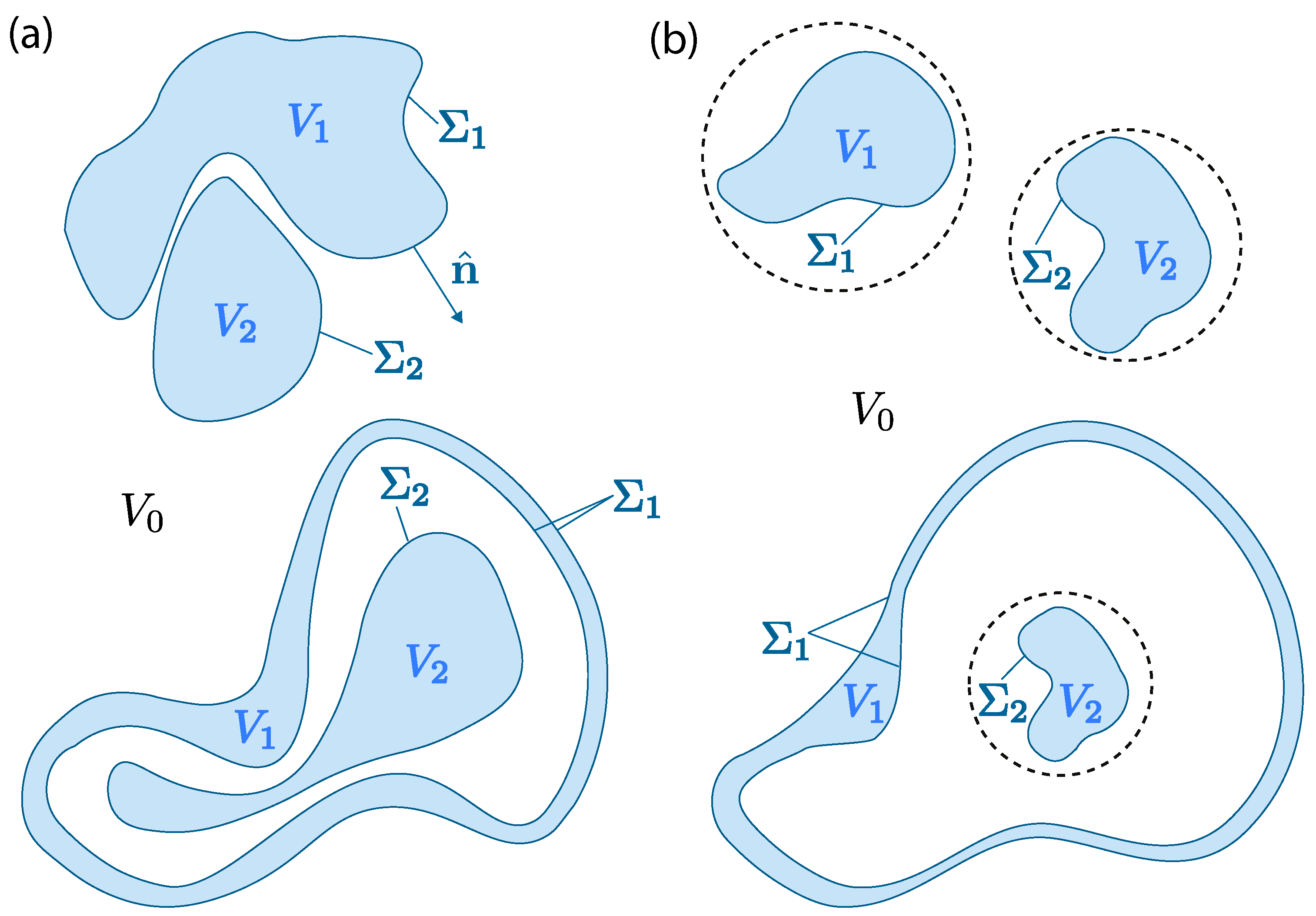
The interaction induced by quantum and thermal fluctuation of the electromagnetic field is an everyday phenomenon that acts between all neutral objects, both on atomic and macroscopic scales [1,2,3,4,5]. For the Casimir interaction between macroscopic bodies, the last two decades have witnessed unparalleled progress in experimental observations and the development of novel theoretical approaches [6,7]. In most of the recent theoretical approaches, the computation of Casimir forces between multiple objects of different shapes and material composition has been achieved by the use of scattering methods or the so-called TGTG formula [8,9,10,11,12,13,14,15,16]. These approaches have the advantage of relatively low numerical effort; they are rapidly converging and can achieve in principle any desired precision [17,18,19,20,21,22]. Another merit of these methods is the exclusion of UV divergencies by performing the subtraction analytically before any numerical computation. Other efficient approaches that have been developed before the scattering approaches include path integral quantizations where the boundary conditions at the surfaces are implemented by delta functions [23]. These approaches are limited to scalar fields with Dirichlet or Neumann boundary conditions [24], or the electromagnetic field with perfectly conducting boundary conditions [25], with the exception of a similar approach for dielectric boundaries [26]. However, such analytical (and semi-analytical) methods have been restricted to symmetric and simple shapes, like spheres, cylinders or ellipsoids [27,28,29,30,31]. Geometries where parts of the bodies interpenetrate, such as those shown in Figure 1a, cannot be studied with scattering approaches. For general shapes and arbitrary geometries, new methods are needed. Purely numerical methods based on surface current fluctuations have been developed [32], but they rely on a full-scale numerical evaluation of matrices and their determinants, which complicates these approaches when high precision of the force is required.

Hence, there is a need to develop methods that predict Casimir interactions between objects of arbitrary geometries composed of materials with arbitrary frequency-dependent electromagnetic properties. The Casimir force can be viewed as arising from the interaction of fluctuating currents distributions. In fact, these effective fluctuating electric and magnetic currents can be considered to be localized either in the bulk of the bodies or just on their surfaces. The surface approach relies on the observation that the electromagnetic response of bodies can be represented entirely in terms of their surfaces, known as the “equivalence principle”, which is based on the observation that many source distributions outside a given region can produce the same field inside the region [33]. The surface approach has been introduced in the literature as a method for a purely numerical computation of Casimir interactions [32]. There are two different methods to implement the idea of computing Casimir forces from fluctuating currents. One can either integrate the Maxwell stress tensor over a closed surface enclosing the body, directly yielding the Casimir force, or integrate over all electromagnetic gauge field fluctuations in a path integral, yielding the Casimir free energy. We shall consider both approaches here.

Compared to scattering theory-based approaches, the surface formulation has the advantage that it does not require the use of eigenfunctions of the vector wave equation that are specific to the shape of the bodies. Hence, our approach is applicable to general geometries and shapes, including interpenetrating structures. In fact, the power of the surface approach has been demonstrated by numerical implementations in Reference [32], where it was used to compute the Casimir force in complicated geometries.

In this paper, we present both the Maxwell stress tensor and path integral-based approaches for the Casimir force and free energy in terms of bulk or surface operators. Our main advancements are

• A new, compact and elegant derivation of the Casimir force from the Maxwell stress tensor within both a T-operator approach and a surface operator approach;
• A new surface formula for the Casimir free energy expressed in terms of a surface operator;
• A new path integral-based derivation of a Lagrange and Hamiltonian formulation for the Casimir free energy.

We also compare the approaches presented here to methods existing in the literature. For the special case of bodies that can be separated by non-overlapping enclosing surfaces, along which one of the coordinates in which the wave equation is separable is constant, our approach is shown to be equivalent to the scattering approach. Our approaches also show the general equivalence of the use of the Maxwell stress tensor in combination with the fluctuation-dissipation theorem on one side and the path integral representation of the Casimir force on the other side. As the most simple application of our approaches, we re-derive the Lifshitz formula for the Casimir free energy of two dielectric slabs. Other analytical applications of our approach will be presented elsewhere.

The geometries and shapes to which our approaches can be applied are shown in Figure 1a. For comparison, in Figure 1b, we display non-penetrating bodies to which scattering theory-based approaches are limited. In general, we assume a configuration composed of N bodies with dielectric functions ${ϵ}_r\left(\omega \right)$ and magnetic permeabilities ${\mu }_r\left(\omega \right)$, $r=1,\dots ,N$. The bodies occupy the volumes $V_r$ with surfaces ${\mathsf{\Sigma }}_r$ and outward pointing surface normal vectors ${\widehat{\mathbf{n}}}_r$. The space with volume $V_0$ in between the bodies is filled by matter with dielectric function ${ϵ}_0\left(\omega \right)$ and magnetic permeability ${\mu }_0\left(\omega \right)$.

2. Stress-Tensor Approach

2.1. Bulk and Surface Expressions for the Force

Consider a collection of N magneto-dielectric bodies in vacuum. In the stress-tensor approach, the (bare) Casimir force $F_i^{\left(\mathrm{bare}\right|r)}$ on body r is obtained by integrating the expectation value $\langle T_{ij}\rangle$ of the Maxwell stress tensor

$$\langle T_{ij}\left(\mathbf{x}\right)\rangle =\frac{1}{4\pi }\left\{\langle E_i\left(\mathbf{x}\right)E_j\left(\mathbf{x}\right)\rangle +\langle H_i\left(\mathbf{x}\right)H_j\left(\mathbf{x}\right)\rangle -\frac{1}{2}{\delta }_{ij}\left[\langle E_k\left(\mathbf{x}\right)E_k\left(\mathbf{x}\right)\rangle +\langle H_k\left(\mathbf{x}\right)H_k\left(\mathbf{x}\right)\rangle \right]\right\}$$

(1)

over any closed surface $S_r$ drawn in the vacuum, which surrounds that body (but excludes all other bodies):

$$F_i^{\left(\mathrm{bare}\right|r)}={\oint }_{S_r}{d}^2\sigma {\widehat{n}}_j\left(\mathbf{x}\right)\langle T_{ji}\left(\mathbf{x}\right)\rangle ,$$

(2)

where $\widehat{\mathbf{n}}$ is the unit normal oriented outside $S_r$, and the angular brackets denote the expectation value taken with respect to quantum and thermal fluctuations. For a system in thermal equilibrium at temperature T, the (equal-time) expectation values of the products of field components (at points $\mathbf{x}$ and ${\mathbf{x}}^{\prime }$ in the vacuum region) are provided by the fluctuation-dissipation theorem [34,35]:

$$\begin{array}{ccc}\hfill \langle {\widehat{E}}_i\left(\mathbf{x}\right){\widehat{E}}_j\left({\mathbf{x}}^{\prime }\right)\rangle & =& 2k_{B}T\sum _{n=0}^{\infty }{}^{\prime }{\mathcal{G}}_{ij}^{\left(EE\right)}(\mathbf{x},{\mathbf{x}}^{\prime };\mathrm{i}{\xi }_n),\hfill \\ \hfill \langle {\widehat{H}}_i\left(\mathbf{x}\right){\widehat{H}}_j\left({\mathbf{x}}^{\prime }\right)\rangle & =& 2k_{B}T\sum _{n=0}^{\infty }{}^{\prime }{\mathcal{G}}_{ij}^{\left(HH\right)}(\mathbf{x},{\mathbf{x}}^{\prime };\mathrm{i}{\xi }_n),\hfill \end{array}$$

(3)

where ${\xi }_n=2\pi n{k}_{B}T/\hslash$ are the Matsubara imaginary frequencies, and the prime in the summations mean that the $n=0$ term is taken with a weight of one half. When the r.h.s of the above equations are plugged into Equation (1), one obtains for $\langle T_{ij}\left(\mathbf{x}\right)\rangle$ a formally divergent expression, since the Green functions ${\mathcal{G}}_{ij}^{\left(\alpha \beta \right)}(\mathbf{x},{\mathbf{x}}^{\prime };\mathrm{i}{\xi }_n)$ are singular in the coincidence limit $\mathbf{x}={\mathbf{x}}^{\prime }$. This divergence can however be easily disposed of by noticing that the Green’s functions admit the decomposition:

$${\mathcal{G}}_{ij}^{\left(\alpha \beta \right)}(\mathbf{x},{\mathbf{x}}^{\prime };\mathrm{i}{\xi }_n)={\mathcal{G}}_{ij}^{(\alpha \beta ;0)}(\mathbf{x}-{\mathbf{x}}^{\prime };\mathrm{i}{\xi }_n)+{\mathsf{\Gamma }}_{ij}^{\left(\alpha \beta \right)}(\mathbf{x},{\mathbf{x}}^{\prime };\mathrm{i}{\xi }_n),$$

(4)

where ${\mathcal{G}}_{ij}^{(\alpha \beta ;0)}(\mathbf{x}-{\mathbf{x}}^{\prime };\mathrm{i}{\xi }_n)$ is the Green’s function of free space, while ${\mathsf{\Gamma }}_{ij}^{\left(\alpha \beta \right)}(\mathbf{x},{\mathbf{x}}^{\prime };\mathrm{i}{\xi }_n)$ describes the effect of scattering of electromagnetic fields by the bodies. In the coincidence limit, only ${\mathcal{G}}_{ij}^{(\alpha \beta ;0)}(\mathbf{x}-{\mathbf{x}}^{\prime };\mathrm{i}{\xi }_n)$ diverges, while ${\mathsf{\Gamma }}_{ij}^{\left(\alpha \beta \right)}(\mathbf{x},{\mathbf{x}}^{\prime };\mathrm{i}{\xi }_n)$ attains a finite limit. When the decomposition in Equation (4) is used to evaluate the r.h.s. of Equation (1), one finds that the expectation value of the stress tensor is decomposed in a way analogous to Equation (4):

$$\langle T_{ij}\left(\mathbf{x}\right)\rangle =\langle T_{ij}^{\left(0\right)}\left(\mathbf{x}\right)\rangle +{\mathsf{\Theta }}_{ij}\left(\mathbf{x}\right),$$

(5)

where $\langle T_{ij}^{\left(0\right)}\left(\mathbf{x}\right)\rangle$ is the divergent expectation value of the stress tensor in empty space, and ${\mathsf{\Theta }}_{ij}\left(\mathbf{x}\right)$ is the finite expression

$$\begin{array}{ccc}\hfill {\mathsf{\Theta }}_{ij}\left(\mathbf{x}\right)& =& \frac{k_{B}T}{2\pi }\sum _{n=0}^{\infty }{}^{\prime }\left[{\mathsf{\Gamma }}_{ij}^{\left(EE\right)}(\mathbf{x},\mathbf{x};\mathrm{i}{\xi }_n)+{\mathsf{\Gamma }}_{ij}^{\left(HH\right)}(\mathbf{x},\mathbf{x};\mathrm{i}{\xi }_n)\right.\hfill \\ & & \left.-\frac{1}{2}{\delta }_{ij}\left({\mathsf{\Gamma }}_{kk}^{\left(EE\right)}(\mathbf{x},\mathbf{x};\mathrm{i}{\xi }_n)+{\mathsf{\Gamma }}_{kk}^{\left(HH\right)}(\mathbf{x},\mathbf{x};\mathrm{i}{\xi }_n)\right)\right].\hfill \end{array}$$

(6)

Since the divergent contribution $\langle T_{ij}^{\left(0\right)}\left(\mathbf{x}\right)\rangle$ is independent of the presence of the bodies, one can just neglect it and then one obtains the following finite expression for the Casimir force on body r due to the presence of the other bodies,

$$F_i^{\left(r\right)}={\oint }_{S_r}{d}^2\sigma {\widehat{n}}_j\left(\mathbf{x}\right){\mathsf{\Theta }}_{ji}\left(\mathbf{x}\right).$$

(7)

The further development of the theory starts from the observation that the dyadic Green’s functions ${\mathsf{\Gamma }}_{ij}^{\left(\alpha \beta \right)}(\mathbf{x},{\mathbf{x}}^{\prime })$ (for brevity, from now on we shall not display the dependence of the Green’s functions on the Matsubara frequencies ${\xi }_n$) can be expressed in two distinct possible forms.

The first representation is general, since it is valid for arbitrary constitutive equations of the magneto-dielectric materials constituting the bodies, which can possibly be non-homogeneous, anisotropic, and non-local. For all points $\mathbf{x}$ and ${\mathbf{x}}^{\prime }$, it expresses ${\mathsf{\Gamma }}_{ij}^{\left(\alpha \beta \right)}(\mathbf{x},{\mathbf{x}}^{\prime })$ in the form of an integral of the T-operator $\widehat{T}$ (for its definition, see Appendix B.1) over the volumeV occupied by all bodies:

$${\mathsf{\Gamma }}_{ij}^{\left(\alpha \beta \right)}(\mathbf{x},{\mathbf{x}}^{\prime })=\sum _{r,r^{\prime }=1}^N{\int }_{V_r}{d}^3\mathbf{y}{\int }_{V_{r^{\prime }}}{d}^3{\mathbf{y}}^{\prime }{\mathcal{G}}_{ik}^{(\alpha \rho ;0)}(\mathbf{x}-\mathbf{y})T_{kl}^{\left(\rho \sigma \right)}(\mathbf{y},{\mathbf{y}}^{\prime }){\mathcal{G}}_{lj}^{(\sigma \beta ;0)}({\mathbf{y}}^{\prime }-{\mathbf{x}}^{\prime }).$$

(8)

The above formula has a simple intuitive interpretation, if one recalls that according to its definition, the T-operator provides the polarization induced in the volume of the bodies when they are immersed in the electromagnetic field generated by a certain distribution of external sources.

The second representation is less general than Equation (8) because it applies only to magneto-dielectric bodies that are (piecewise) homogeneous and isotropic 1. It expresses ${\mathsf{\Gamma }}_{ij}^{\left(\alpha \beta \right)}(\mathbf{x},{\mathbf{x}}^{\prime })$ in the form of an integral of the surface operator ${\widehat{M}}^{-1}$ defined in Equation (A44), over the union $\mathsf{\Sigma }=\bigcup {\mathsf{\Sigma }}_r$ of the surfaces ${\mathsf{\Sigma }}_r$ of the bodies. For two points $\mathbf{x}$ and ${\mathbf{x}}^{\prime }$ both lying in the vacuum region outside the bodies2, the surface representation of ${\mathsf{\Gamma }}_{ij}^{\left(\alpha \beta \right)}(\mathbf{x},{\mathbf{x}}^{\prime })$ reads:

$$\begin{array}{ccc}\hfill {\mathsf{\Gamma }}_{ij}^{\left(\alpha \beta \right)}(\mathbf{x},{\mathbf{x}}^{\prime })& =& -\sum _{r,r^{\prime }=1}^N{\int }_{V_r}{d}^3\mathbf{y}{\int }_{V_{r^{\prime }}}{d}^3{\mathbf{y}}^{\prime }\delta \left(F_r\left(\mathbf{y}\right)\right)\delta \left(F_{r^{\prime }}\left({\mathbf{y}}^{\prime }\right)\right)\hfill \\ & \times & {\mathcal{G}}_{ik}^{(\alpha \rho ;0)}(\mathbf{x}-\mathbf{y})){\left(M^{-1}\right)}_{kl}^{\left(\rho \sigma \right)}(\mathbf{y},{\mathbf{y}}^{\prime }){\mathcal{G}}_{lj}^{(\sigma \beta ;0)}({\mathbf{y}}^{\prime }-{\mathbf{x}}^{\prime }),\hfill \end{array}$$

(9)

where $F_r\left(\mathbf{y}\right)=0$ is the equation of the surface ${\mathsf{\Sigma }}_r$. This representation also has a simple intuitive meaning, if one considers that $-{\widehat{M}}^{-1}$ (see Appendix B.2 for details) is defined as the operator that provides the fictitious surface polarizations that radiate outside the bodies the same scattered electromagnetic field as the one radiated by the physically induced volumic polarization, in response to an external field. The derivations of Equations (8) and (9) are presented in Appendix B. It is apparent that both representations have the same mathematical structure, consisting of a two-sided convolution of a certain kernel ${\mathcal{K}}_{ij}^{\left(\alpha \beta \right)}(\mathbf{x},{\mathbf{x}}^{\prime })$ with the free-space Green’s functions ${\mathcal{G}}_{ij}^{(\alpha \beta ;0)}(\mathbf{x}-{\mathbf{x}}^{\prime })$:

$${\mathsf{\Gamma }}_{ij}^{\left(\alpha \beta \right)}(\mathbf{x},{\mathbf{x}}^{\prime })={\int }_V{d}^3\mathbf{y}{\int }_V{d}^3{\mathbf{y}}^{\prime }{\mathcal{G}}_{ik}^{(\alpha \rho ;0)}(\mathbf{x}-\mathbf{y}){\mathcal{K}}_{kl}^{\left(\rho \sigma \right)}(\mathbf{y},{\mathbf{y}}^{\prime }){\mathcal{G}}_{lj}^{(\sigma \beta ;0)}({\mathbf{y}}^{\prime }-{\mathbf{x}}^{\prime }).$$

(10)

The only difference between the two representations consists in the expression of $\mathcal{K}$, which in the case of Equation (8) is the three-dimensional kernel $T_{kl}^{\left(\rho \sigma \right)}(\mathbf{y},{\mathbf{y}}^{\prime })$ supported in the volume V occupied by the bodies:

$${\mathcal{K}}_{kl}^{\left(\rho \sigma \right)}(\mathbf{y},{\mathbf{y}}^{\prime })=T_{kl}^{\left(\rho \sigma \right)}(\mathbf{y},{\mathbf{y}}^{\prime }),$$

(11)

while in Equation (9) $\mathcal{K}$ is the two-dimensional kernel $-{\left(M^{-1}\right)}_{kl}^{\left(\rho \sigma \right)}(\mathbf{y},{\mathbf{y}}^{\prime })$ supported on the union $\mathsf{\Sigma }$ of their surfaces:

$${\mathcal{K}}_{kl}^{\left(\rho \sigma \right)}(\mathbf{y},{\mathbf{y}}^{\prime })=-\sum _{r,r^{\prime }=1}^N\delta \left(F_r\left(\mathbf{y}\right)\right)\delta \left(F_{r^{\prime }}\left({\mathbf{y}}^{\prime }\right)\right){\left(M^{-1}\right)}_{kl}^{\left(\rho \sigma \right)}(\mathbf{y},{\mathbf{y}}^{\prime })$$

(12)

In both cases, the above equation can be concisely written using the operator notation described in Appendix A:

$$\widehat{\mathsf{\Gamma }}={\widehat{\mathcal{G}}}^{\left(0\right)}\widehat{\mathcal{K}}{\widehat{\mathcal{G}}}^{\left(0\right)}.$$

(13)

In Appendix C, we prove that the structure of the representation of ${\mathsf{\Gamma }}_{ij}^{\left(\alpha \beta \right)}(\mathbf{x},{\mathbf{x}}^{\prime })$ given in Equation (10), allows to re-express the Casimir force Equation (7) in the following remarkably simple form:

$$F_i^{\left(r\right)}=2k_{B}T\sum _{n=0}^{\infty }{}^{\prime }{\int }_{V_r}{d}^3\mathbf{y}{\int }_V{d}^3{\mathbf{y}}^{\prime }\left({\mathcal{K}}_{lj}^{\left(\alpha \beta \right)}({\mathbf{y}}^{\prime },\mathbf{y};\mathrm{i}{\xi }_n)\frac{\partial }{\partial y_i}{\mathcal{G}}_{jl}^{(\beta \alpha ;0)}(\mathbf{y}-{\mathbf{y}}^{\prime };\mathrm{i}{\xi }_n)\right).$$

(14)

A crucial role in the derivation of Equation (14) is played by the fact that the kernel $\mathcal{K}$ satisfies a set of reciprocity relations analogous to those satisfied by the Green’s functions:

$${\mathcal{K}}_{kl}^{\left(\rho \sigma \right)}(\mathbf{y},{\mathbf{y}}^{\prime })={(-1)}^{s\left(\rho \right)+s\left(\sigma \right)}{\mathcal{K}}_{lk}^{\left(\sigma \rho \right)}({\mathbf{y}}^{\prime },\mathbf{y}),$$

(15)

where $s\left(E\right)=0$ and $s\left(H\right)=1$. It is possible to verify that the reciprocity relations satisfied by ${\mathcal{G}}_{ij}^{(\alpha \beta ;0)}(\mathbf{y}-{\mathbf{y}}^{\prime })$ and ${\mathcal{K}}_{ij}^{\left(\alpha \beta \right)}(\mathbf{y},{\mathbf{y}}^{\prime })$ ensure vanishing of the “self-force” $F_i^{\left(\mathrm{self}\right|r)}$:

$$F_i^{\left(\mathrm{self}\right|r)}=2k_{B}T\sum _{n=0}^{\infty }{}^{\prime }{\int }_{V_r}{d}^3\mathbf{y}{\int }_{V_r}{d}^3{\mathbf{y}}^{\prime }\left({\mathcal{K}}_{ij}^{\left(\alpha \beta \right)}({\mathbf{y}}^{\prime },\mathbf{y};\mathrm{i}{\xi }_n)\frac{\partial }{\partial y_i}{\mathcal{G}}_{ji}^{(\beta \alpha ;0)}(\mathbf{y}-{\mathbf{y}}^{\prime };\mathrm{i}{\xi }_n)\right)=0.$$

(16)

This implies that in Equation (14) the ${\mathbf{y}}^{\prime }$ integral is in fact restricted to $V-V_r$, in accord with one’s intuition that the force on body r is due to the interaction with the other bodies. It is possible to present Equation (14) in a more compact and symmetric form, by defining the derivative $\partial /\partial {\mathbf{x}}_r$ of any kernel $\mathcal{A}(\mathbf{y},{\mathbf{y}}^{\prime })$, with respect to rigid translations of the r-th body:

$$\frac{\partial }{\partial {\mathbf{x}}_r}\mathcal{A}(\mathbf{y},{\mathbf{y}}^{\prime })\equiv {\psi }_r\left(\mathbf{y}\right)\frac{\partial }{\partial \mathbf{y}}\mathcal{A}(\mathbf{y},{\mathbf{y}}^{\prime })+{\psi }_r\left({\mathbf{y}}^{\prime }\right)\frac{\partial }{\partial {\mathbf{y}}^{\prime }}\mathcal{A}(\mathbf{y},{\mathbf{y}}^{\prime }),$$

(17)

where ${\psi }_r\left(\mathbf{y}\right)$ is the characteristic function of $V_r$: ${\psi }_r\left(\mathbf{y}\right)=1$ if $\mathbf{y}\in V_r$, ${\psi }_r\left(\mathbf{y}\right)=0$ if $\mathbf{y}\notin V_r$. Using $\partial /\partial {\mathbf{x}}_r$, we can rewrite Equation (14) as

$${\mathbf{F}}^{\left(r\right)}=k_{B}T\sum _{n=0}^{\infty }{}^{\prime }{\int }_V{d}^3\mathbf{y}{\int }_V{d}^3{\mathbf{y}}^{\prime }\left({\mathcal{K}}_{ij}^{\left(\alpha \beta \right)}({\mathbf{y}}^{\prime },\mathbf{y};\mathrm{i}{\xi }_n)\frac{\partial }{\partial {\mathbf{x}}_r}{\mathcal{G}}_{ji}^{(\beta \alpha ;0)}(\mathbf{y}-{\mathbf{y}}^{\prime };\mathrm{i}{\xi }_n)\right).$$

(18)

The expression on the r.h.s. of the above formula can be compactly expressed using the operator notation and the trace operation described in Appendix A:

$${\mathbf{F}}^{\left(r\right)}=k_{B}T\sum _{n=0}^{\infty }{}^{\prime }\mathrm{Tr}\left[\widehat{\mathcal{K}}\left(\mathrm{i}{\xi }_n\right)\frac{\partial }{\partial {\mathbf{x}}_r}{\widehat{\mathcal{G}}}^{\left(0\right)}\left(\mathrm{i}{\xi }_n\right)\right].$$

(19)

Depending on whether we use for the kernel $\widehat{K}$ the T-operator of Equation (8) or rather the surface operator $-\widehat{M}$ of Equation (9), Equation (19) provides us with two distinct but formally similar representations of the Casimir force, which is expressed either as an integral over the volume V occupied by the bodies or as an integral over their surfaces $\mathsf{\Sigma }$. One feature of Equation (19) is worth stressing. Since the force is expressed as a trace, Equation (19) can be evaluated in an arbitrary basis, leaving one with complete freedom in the choice of the most convenient basis in a concrete situation. A representation of the Casimir force in the form of a volume integral equivalent to Equation (19) was derived in [11], while the surface-integral representation was obtained in [32]. Equation (19) can be computed numerically for any shapes and dispositions of the bodies, by using discrete meshes covering the bodies. An efficient numerical scheme based on surface-elements methods is described in [32], where it was used to compute the Casimir force in complex geometries, not amenable to analytical techniques.

2.2. Casimir Free Energy

In this section, we compute the Casimir free energy $\mathcal{F}$ of the system of bodies, starting from the force formula Equation (19). We shall see that the T-operator and the surface-operator approaches lead to two distinct but equivalent representations of the Casimir energy.

2.2.1. T-Operator Approach

Plugging into Equation (19) the expression of the T-operator Equation (A36), we find that the Casimir force can be expressed in the form:

$${\mathbf{F}}^{\left(r\right)}=k_{B}T\sum _{n=0}^{\infty }{}^{\prime }\mathrm{Tr}\left(\widehat{T}\left(\mathrm{i}{\xi }_n\right)\frac{\partial }{\partial {\mathbf{x}}_r}{\widehat{\mathcal{G}}}^{\left(0\right)}\left(\mathrm{i}{\xi }_n\right)\right)=k_{B}T\sum _{n=0}^{\infty }{}^{\prime }\mathrm{Tr}\left[\frac{1}{1-\widehat{\chi }{\widehat{\mathcal{G}}}^{\left(0\right)}}\frac{\partial }{\partial {\mathbf{x}}_r}\left(\widehat{\chi }{\widehat{\mathcal{G}}}^{\left(0\right)}\right)\right],$$

(20)

where in the last passage, we made use of the fact that the polarization operator $\widehat{\chi }$ defined in Equation (A24) is invariant under a rigid displacement of the body. The r.h.s. of the above equation can be formally expressed as a gradient:

$$F^{\left(r\right)}=-\frac{\partial }{\partial {\mathbf{x}}_r}{\mathcal{F}}_{\mathrm{bare}},$$

(21)

where ${\mathcal{F}}_{\mathrm{bare}}$ is the bare free energy:

$${\mathcal{F}}_{\mathrm{bare}}=k_{B}T\sum _{n=0}^{\infty }{}^{\prime }\mathrm{Tr}log[1-\widehat{\chi }{\widehat{\mathcal{G}}}^{\left(0\right)}]$$

(22)

Unfortunately, ${\mathcal{F}}_{\mathrm{bare}}$ is formally divergent. To obtain the finite Casimir free energy $\mathcal{F}$, one has to subtract from ${\mathcal{F}}_{\mathrm{bare}}$ the divergent self-energies ${\mathcal{F}}_{\mathrm{self}}^{\left(r\right)}$ of the individual bodies:

$${\mathcal{F}}_{\mathrm{self}}^{\left(r\right)}=\left\{k_{B}T\sum _{n=0}^{\infty }{}^{\prime }\mathrm{Tr}log[1-{\widehat{\chi }}_r{\widehat{\mathcal{G}}}^{\left(0\right)}]\right\},$$

(23)

where ${\widehat{\chi }}_r={\widehat{\psi }}_r\widehat{\chi }{\widehat{\psi }}_r$ is the polarizability operator of body r in isolation. In the case of a system composed by two bodies, the renormalized Casimir free energy can be recast in the following TGTG form:

$$\mathcal{F}={\mathcal{F}}_{\mathrm{bare}}-{\mathcal{F}}_{\mathrm{self}}^{\left(1\right)}-{\mathcal{F}}_{\mathrm{self}}^{\left(2\right)}=k_{B}T\sum _{n=0}^{\infty }{}^{\prime }\mathrm{Tr}log[1-{\widehat{T}}_1{\widehat{\mathcal{G}}}^{\left(0\right)}{\widehat{T}}_2{\widehat{\mathcal{G}}}^{\left(0\right)}],$$

(24)

where

$${\widehat{T}}_r=\frac{1}{1-{\widehat{\chi }}_r{\widehat{\mathcal{G}}}^{\left(0\right)}}{\widehat{\chi }}_r,$$

(25)

is the T-operator of body r in isolation. To prove Equation (24), one notes that for each Matsubara mode the operator identity holds:

$$(1-{\widehat{\mathcal{G}}}^{\left(0\right)}{\widehat{\chi }}_1){\widehat{\mathcal{G}}}^{\left(0\right)}{\widehat{T}}_1{\widehat{\mathcal{G}}}^{\left(0\right)}{\widehat{T}}_2(1-{\widehat{\mathcal{G}}}^{\left(0\right)}{\widehat{\chi }}_2)={\widehat{\mathcal{G}}}^{\left(0\right)}{\widehat{\chi }}_1{\widehat{\mathcal{G}}}^{\left(0\right)}{\widehat{\chi }}_2.$$

(26)

The above identity in turn allows to prove the following chain of identities:

$$\mathrm{Tr}log[1-{\widehat{\mathcal{G}}}^{\left(0\right)}{\widehat{\chi }}_1]+\mathrm{Tr}log[1-{\widehat{\mathcal{G}}}^{\left(0\right)}{\widehat{T}}_1{\widehat{\mathcal{G}}}^{\left(0\right)}{\widehat{T}}_2]+\mathrm{Tr}log[1-{\widehat{\mathcal{G}}}^{\left(0\right)}{\widehat{\chi }}_2]$$

$$=\mathrm{Tr}log\left[(1-{\widehat{\mathcal{G}}}^{\left(0\right)}{\widehat{\chi }}_1)(1-{\widehat{\mathcal{G}}}^{\left(0\right)}{\widehat{T}}_1{\widehat{\mathcal{G}}}^{\left(0\right)}{\widehat{T}}_2)(1-{\widehat{\mathcal{G}}}^{\left(0\right)}{\widehat{\chi }}_2)\right]$$

$$=\mathrm{Tr}log[(1-{\widehat{\mathcal{G}}}^{\left(0\right)}{\widehat{\chi }}_1)(1-{\widehat{\mathcal{G}}}^{\left(0\right)}{\widehat{\chi }}_2)-(1-{\widehat{\mathcal{G}}}^{\left(0\right)}{\widehat{\chi }}_1){\widehat{\mathcal{G}}}^{\left(0\right)}{\widehat{T}}_1{\widehat{\mathcal{G}}}^{\left(0\right)}{\widehat{T}}_2(1-{\widehat{\mathcal{G}}}^{\left(0\right)}{\widehat{\chi }}_2)]$$

$$=\mathrm{Tr}log[(1-{\widehat{\mathcal{G}}}^{\left(0\right)}{\widehat{\chi }}_1)(1-{\widehat{\mathcal{G}}}^{\left(0\right)}{\widehat{\chi }}_2)-{\widehat{\mathcal{G}}}^{\left(0\right)}{\widehat{\chi }}_1{\widehat{\mathcal{G}}}^{\left(0\right)}{\widehat{\chi }}_2]=\mathrm{Tr}log[(1-{\widehat{\mathcal{G}}}^{\left(0\right)}({\widehat{\chi }}_1+{\widehat{\chi }}_2)]$$

$$=\mathrm{Tr}log[1-{\widehat{\mathcal{G}}}^{\left(0\right)}\widehat{\chi }].$$

(27)

Equating the first line with the last line, we obtain the identity:

$$\begin{array}{ccc}& & \mathrm{Tr}log[1-{\widehat{\mathcal{G}}}^{\left(0\right)}\widehat{\chi }]\hfill \\ & & =\mathrm{Tr}log[1-{\widehat{\mathcal{G}}}^{\left(0\right)}{\widehat{\chi }}_1]+\mathrm{Tr}log[1-{\widehat{\mathcal{G}}}^{\left(0\right)}{\widehat{T}}_1{\widehat{\mathcal{G}}}^{\left(0\right)}{\widehat{T}}_2]+\mathrm{Tr}log[1-{\widehat{\mathcal{G}}}^{\left(0\right)}{\widehat{\chi }}_2].\hfill \end{array}$$

(28)

Upon summing the above identity over all Matsubara modes (with weight one half for the $n=0$ term), and then multiplying it by $k_{B}T$, we find:

$${\mathcal{F}}_{\mathrm{self}}^{\left(1\right)}+{\mathcal{F}}_{\mathrm{self}}^{\left(2\right)}+\mathcal{F}={\mathcal{F}}_{\mathrm{bare}},$$

(29)

which is equivalent to Equation (24). The energy formula Equation (24) was derived in [13] using the path-integral method and in [11], using Rytov’s fluctuational electrodynamics [36].

2.2.2. Surface Operator Approach

Now we derive the surface-operator representation of the Casimir energy. To do that, we start from the surface-operator representation of the force, which is obtained by replacing $\widehat{K}$ in Equation (19) with minus the inverse of the surface operator $\widehat{M}$ defined in Equation (A44):

$${\mathbf{F}}^{\left(r\right)}=-k_{B}T\sum _{n=0}^{\infty }{}^{\prime }\mathrm{Tr}\left[{\widehat{M}}^{-1}\left(\mathrm{i}{\xi }_n\right)\frac{\partial }{\partial {\mathbf{x}}_r}{\widehat{\mathcal{G}}}^{\left(0\right)}\left(\mathrm{i}{\xi }_n\right)\right].$$

(30)

This can also be written as:

$${\mathbf{F}}^{\left(r\right)}=-k_{B}T\sum _{n=0}^{\infty }{}^{\prime }\mathrm{Tr}\left[{\widehat{M}}^{-1}\left(\mathrm{i}{\xi }_n\right)\frac{\partial }{\partial {\mathbf{x}}_r}\left(\widehat{\mathsf{\Pi }}{\widehat{\mathcal{G}}}^{\left(0\right)}\left(\mathrm{i}{\xi }_n\right)\widehat{\mathsf{\Pi }}\right)\right],$$

(31)

where $\widehat{\mathsf{\Pi }}$ is the tangential projection operator defined in Appendix B.2. Now, one notes the identity:

$$\frac{\partial }{\partial {\mathbf{x}}_r}\left(\widehat{\mathsf{\Pi }}{\widehat{\mathcal{G}}}^{\left(0\right)}\left(\mathrm{i}{\xi }_n\right)\widehat{\mathsf{\Pi }}\right)=\frac{\partial \widehat{M}}{\partial {\mathbf{x}}_r},$$

(32)

which is a direct consequence of Equation (A44) since

$$\frac{\partial }{\partial {\mathbf{x}}_r}\sum _{s=1}^N{\widehat{\mathsf{\Pi }}}_s{\widehat{\mathcal{G}}}^{\left(s\right)}{\widehat{\mathsf{\Pi }}}_s=0.$$

(33)

Plugging Equation (32) into Equation (31), we obtain:

$$F^{\left(r\right)}=-k_{B}T\sum _{n=0}^{\infty }{}^{\prime }\mathrm{Tr}\left[{\widehat{M}}^{-1}\left(\mathrm{i}{\xi }_n\right)\frac{\partial }{\partial {\mathbf{x}}_r}\widehat{M}\left(\mathrm{i}{\xi }_n\right)\right],$$

(34)

The r.h.s. of the above equation can be formally expressed as a gradient:

$$F^{\left(r\right)}=-\frac{\partial }{\partial {\mathbf{x}}_r}{\tilde{\mathcal{F}}}_{\mathrm{bare}},$$

(35)

where ${\tilde{\mathcal{F}}}_{\mathrm{bare}}$ is the bare free energy:

$${\tilde{\mathcal{F}}}_{\mathrm{bare}}=k_{B}T\sum _{n=0}^{\infty }{}^{\prime }\mathrm{Tr}log\widehat{M}\left(\mathrm{i}{\xi }_n\right).$$

(36)

Similarly to what we found in the T-operator approach, the surface formula of the bare-energy ${\tilde{\mathcal{F}}}_{\mathrm{bare}}$ is formally divergent. The finite Casimir free energy is obtained by subtracting from ${\tilde{\mathcal{F}}}_{\mathrm{bare}}$ the limit ${\tilde{\mathcal{F}}}_{\mathrm{bare}}^{(\infty )}$ of the bare energy when the bodies are taken infinitely apart from each other. From Equation (A44), one sees that in the limit of infinite separations, the operator $\widehat{M}$ approaches the limit ${\widehat{M}}_{\infty }$

$${\widehat{M}}_{\infty }=\sum _{r=1}^N{\widehat{M}}_r,$$

(37)

where

$${\widehat{M}}_r={\widehat{\mathsf{\Pi }}}_r({\widehat{\mathcal{G}}}^{\left(r\right)}+{\widehat{\mathcal{G}}}^{\left(0\right)}){\widehat{\mathsf{\Pi }}}_r.$$

(38)

Notice that the surface operator ${\widehat{M}}_r$ is localized onto the surface ${\mathsf{\Sigma }}_r$ of the r-th body. This implies that:

$${\widehat{M}}_r{\widehat{M}}_s=0,\mathrm{for}r\ne s.$$

(39)

Using Equation (37), we find that ${\tilde{\mathcal{F}}}_{\mathrm{bare}}^{(\infty )}$ is the formally divergent quantity:

$${\tilde{\mathcal{F}}}_{\mathrm{bare}}^{(\infty )}=k_{B}T\sum _{n=0}^{\infty }{}^{\prime }\mathrm{Tr}log{\widehat{M}}_{\infty }\left(\mathrm{i}{\xi }_n\right)=\sum _{r=1}^N{k}_{B}T\sum _{n=0}^{\infty }{}^{\prime }\mathrm{Tr}log{\widehat{M}}_r\left(\mathrm{i}{\xi }_n\right)\equiv \sum _{r=1}^N{\tilde{\mathcal{F}}}_{\mathrm{self}}^{\left(r\right)}.$$

(40)

The additive character of ${\tilde{\mathcal{F}}}_{\mathrm{bare}}^{(\infty )}$ allows to interpret ${\tilde{\mathcal{F}}}_{\mathrm{self}}^{\left(r\right)}$ as representing the (infinite) the self-energy of the bodies in the surface approach. Upon subtracting Equation (40) from Equation (36), we arrive at the following formula for the Casimir energy:

$$\mathcal{F}=k_{B}T\sum _{n=0}^{\infty }{}^{\prime }logdet\frac{\widehat{M}\left(\mathrm{i}{\xi }_n\right)}{{\widehat{M}}_{\infty }\left(\mathrm{i}{\xi }_n\right)}.$$

(41)

An easy computation shows that

$$\frac{1}{{\widehat{M}}_{\infty }}\widehat{M}=1+\sum _{r\ne s}\frac{1}{{\widehat{M}}_r}{\widehat{\mathcal{G}}}_{rs}^{\left(0\right)}.$$

(42)

where

$${\widehat{\mathcal{G}}}_{rs}^{\left(0\right)}={\widehat{\mathsf{\Pi }}}_r{\widehat{\mathcal{G}}}^{\left(0\right)}{\widehat{\mathsf{\Pi }}}_s.$$

(43)

Substitution of the above formula into Equation (41) results in the following surface formula for the Casimir energy:

$$\mathcal{F}=k_{B}T\sum _{n=0}^{\infty }{}^{\prime }logdet\left[1+\sum _{r\ne s}\frac{1}{{\widehat{M}}_r}{\widehat{\mathcal{G}}}_{rs}^{\left(0\right)}\right].$$

(44)

In the simple case of two bodies, the above formula reduces to:

$$\mathcal{F}=k_{B}T\sum _{n=0}^{\infty }{}^{\prime }\mathrm{Tr}log\left[1-\frac{1}{{\widehat{M}}_1}{\widehat{\mathcal{G}}}_{12}^{\left(0\right)}\frac{1}{{\widehat{M}}_2}{\widehat{\mathcal{G}}}_{21}^{\left(0\right)}\right].$$

(45)

The surface formulas for the Casimir energy given in Equations (44) and (45) were not known before and are presented here for the first time. Comparison of Equation (45) with Equation (24) reveals the striking similarity of the T-operator and surface-approach representations of the Casimir energy. Indeed we see that both formulas can be written in the form:

$$\mathcal{F}=k_{B}T\sum _{n=0}^{\infty }{}^{\prime }\mathrm{Tr}log\left[1-{\widehat{\mathcal{K}}}_1{\widehat{\mathcal{G}}}^{\left(0\right)}{\widehat{\mathcal{K}}}_2{\widehat{\mathcal{G}}}^{\left(0\right)}\right],$$

(46)

where ${\widehat{\mathcal{K}}}_r$ is the kernel, which gives the scattering Green’s function of body r in isolation:

$${\widehat{\mathsf{\Gamma }}}_r={\widehat{\mathcal{G}}}^{\left(0\right)}{\widehat{\mathcal{K}}}_r{\widehat{\mathcal{G}}}^{\left(0\right)}.$$

(47)

3. Equivalence of the Surface-Formula with the Scattering Formula for the Casimir Energy

In the previous sections, we have shown that, both in the T-operator and in the surface approaches, the Casimir energy $\mathcal{F}$ of two bodies can be expressed by the general Equation (46). This formula is valid for any shape and relative dispositions of the two bodies, and in particular for two interleaved bodies (see Figure 1a). Now we show that when the two bodies can be enclosed within two non-overlapping spheres (see Figure 1b), Equation (46) is the same as the well-known scattering formula [8,9,10,11,12]:

$$\mathcal{F}=k_{B}T\sum _{n=0}^{\infty }{}^{\prime }\mathrm{tr}log\left[1-{\mathcal{T}}^{\left(1\right)}{\mathcal{U}}^{\left(12\right)}{\mathcal{T}}^{\left(2\right)}{\mathcal{U}}^{\left(21\right)}\right].$$

(48)

where ${\mathcal{T}}^{\left(r\right)}$ is the scattering matrix of body r (see Equation (A76) for the definition of ${\mathcal{T}}^{\left(r\right)}$), ${\mathcal{U}}^{\left(rs\right)}$ are the translation matrices defined in Equation (A82) and $\mathrm{tr}$ denotes a trace over multipole indices.

To prove equivalence of Equation (46) with Equation (48), one starts from the observation that the trace operation in Equation (46) involves evaluating the Green functions ${\overleftrightarrow{\mathcal{G}}}^{(\alpha \beta ;0)}(\mathbf{y},{\mathbf{y}}^{\prime })$ at points $\mathbf{y}$ and ${\mathbf{y}}^{\prime }$, one of which (call it ${\mathbf{y}}_1$) belongs to body 1, while the other (call it ${\mathbf{y}}_2$) belongs to body 2. For two bodies that can be separated by non-overlapping spheres, it is warranted that $|{\mathbf{y}}_1-{\mathbf{X}}_1|<|{\mathbf{y}}_2-{\mathbf{X}}_1|$ and $|{\mathbf{y}}_2-{\mathbf{X}}_2|<|{\mathbf{y}}_1-{\mathbf{X}}_2|$, where ${\mathbf{X}}_1$ and ${\mathbf{X}}_2$ are the positions of the centers of the spheres $S^{\left(1\right)}$ and $S^{\left(2\right)}$, respectively, and $d=|{\mathbf{X}}_2-{\mathbf{X}}_1|$ is their distance. This condition satisfied by ${\mathbf{y}}_1$ and ${\mathbf{y}}_2$ ensures that it is legitimate to express ${\overleftrightarrow{\mathcal{G}}}^{(\alpha \beta ;0)}({\mathbf{y}}_r,{\mathbf{y}}_s)$ (with $r\ne s=1,2$) by the partial-wave expansion (see Appendix D):

$$\begin{array}{ccc}\hfill {\overleftrightarrow{\mathcal{G}}}^{(\alpha \beta ;0)}({\mathbf{y}}_r,{\mathbf{y}}_s)& =& \lambda {(-1)}^{s\left(\beta \right)}\sum _{plm}{\mathsf{\Phi }}_{plm}^{\left(\alpha \right|\mathrm{reg})}({\mathbf{y}}_r-{\mathbf{X}}_r)\otimes {\mathsf{\Phi }}_{pl-m}^{\left(\beta \right|\mathrm{out})}({\mathbf{y}}_s-{\mathbf{X}}_r)\hfill \\ & =& \lambda {(-1)}^{s\left(\beta \right)}\sum _{plm}\sum _{p^{\prime }{l}^{\prime }}{\mathsf{\Phi }}_{plm}^{\left(\alpha \right|\mathrm{reg})}({\mathbf{y}}_r-{\mathbf{X}}_r)\otimes {\mathcal{U}}_{pl;p^{\prime }{l}^{\prime }}^{\left(rs\right)}\left(d\right){\mathsf{\Phi }}_{p^{\prime }{l}^{\prime }-m}^{\left(\beta \right|\mathrm{reg})}({\mathbf{y}}_s-{\mathbf{X}}_s),\hfill \end{array}$$

(49)

where ${\mathsf{\Phi }}_{plm}^{(\mathrm{reg}/\mathrm{out})}({\mathbf{y}}_r-{\mathbf{X}}_r)$ are a basis of regular and outgoing spherical waves with origin at ${\mathbf{X}}_r$. When the above expansion is substituted into Equation (46) and the trace is evaluated, one finds that $\mathcal{F}$ can be recast in the form:

$$\mathcal{F}=k_{B}T\sum _{n=0}^{\infty }{}^{\prime }\mathrm{tr}log\left[1-\mathcal{N}\right].$$

(50)

where $\mathcal{N}$ is the matrix of elements:

$$\begin{array}{ccc}& & {\mathcal{N}}_{plm;p^{\prime }{l}^{\prime }{m}^{\prime }}\equiv \sum _{p^{\prime \prime }{l}^{\prime \prime }}\sum _{p^{\prime \prime \prime }{l}^{\prime \prime \prime }{m}^{\prime \prime \prime }}\sum _{p^{\prime \prime \prime \prime }{l}^{\prime \prime \prime \prime }}{\mathcal{U}}_{pl,p^{\prime \prime }{l}^{\prime \prime }}^{\left(21\right)}\left(d\right){\mathcal{U}}_{p^{\prime \prime \prime }{l}^{\prime \prime \prime };p^{\prime \prime \prime \prime }{l}^{\prime \prime \prime \prime }}^{\left(12\right)}\left(d\right)\hfill \\ & \times & \lambda \sum _{\alpha ,\mu }{(-1)}^{s\left(\alpha \right)}{\int }_{V_1}{d}^3{\mathbf{y}}_1{\int }_{V_1}{d}^3{\mathbf{y}}_1^{\prime }{\mathsf{\Phi }}_{p^{\prime \prime }{l}^{\prime \prime }-m}^{\left(\alpha \right|\mathrm{reg})}({\mathbf{y}}_1-{\mathbf{X}}_1)·{\overleftrightarrow{\mathcal{K}}}_1^{\left(\alpha \mu \right)}({\mathbf{y}}_1,{\mathbf{y}}_1^{\prime })·{\mathsf{\Phi }}_{p^{\prime \prime \prime }{l}^{\prime \prime \prime }{m}^{\prime \prime \prime }}^{\left(\mu \right|\mathrm{reg})}({\mathbf{y}}_1^{\prime }-{\mathbf{X}}_1)\hfill \\ & \times & \lambda \sum _{\beta ,\nu }{(-1)}^{s\left(\nu \right)}{\int }_{V_2}{d}^3{\mathbf{y}}_2{\int }_{V_2}{d}^3{\mathbf{y}}_2^{\prime }{\mathsf{\Phi }}_{p^{\prime \prime \prime \prime }{l}^{\prime \prime \prime \prime }-m^{\prime \prime \prime }}^{\left(\nu \right|\mathrm{reg})}({\mathbf{y}}_2-{\mathbf{X}}_2)·{\overleftrightarrow{\mathcal{K}}}_2^{\left(\nu \beta \right)}({\mathbf{y}}_2,{\mathbf{y}}_2^{\prime })·{\mathsf{\Phi }}_{p^{\prime }{l}^{\prime }{m}^{\prime }}^{\left(\beta \right|\mathrm{reg})}({\mathbf{y}}_2^{\prime }-{\mathbf{X}}_2).\hfill \end{array}$$

Recalling the formula Equation (A79) for the scattering matrices ${\mathcal{T}}^{\left(r\right)}$ of the two bodies, we see that $\mathcal{N}$ is the matrix:

$$\mathcal{N}={\mathcal{U}}^{\left(21\right)}\left(d\right){\mathcal{T}}^{\left(1\right)}{\mathcal{U}}^{\left(12\right)}\left(d\right){\mathcal{T}}^{\left(2\right)}.$$

(51)

Upon substituting the above expression into the r.h.s. of Equation (50), and using cyclicity of the trace, we see that Equation (50) indeed coincides with the scattering formula Equation (48).

4. Path Integral Approach

As in the previous sections, we consider again N dielectric bodies occupying the volumes $V_r$, $r=1,\dots ,N$, bounded by surfaces ${\mathsf{\Sigma }}_r$. Their electromagnetic properties are described by the dielectric functions ${ϵ}^{\left(r\right)}$ and magnetic permeability ${\mu }^{\left(r\right)}$. The bodies are embedded in a homogeneous medium occupying the outside volume of the bodies, $V_0$, with dielectric function ${ϵ}^{\left(0\right)}$ and magnetic permeability ${\mu }^{\left(0\right)}$.

In the Euclidean path integral quantization of the electromagnetic field, the Casimir free energy at finite temperature T can be obtained as

$$\mathcal{F}=-k_{B}T\sum _{n=0}^{\infty }{}^{\prime }log\frac{\mathcal{Z}\left({\kappa }_n\right)}{{\mathcal{Z}}_{\infty }\left({\kappa }_n\right)},$$

(52)

where the sum runs over the Matsubara momenta ${\kappa }_n=2\pi n{k}_{B}T/\hslash c$, with a weight of $1/2$ for $n=0$. The partition function $\mathcal{Z}$ is given by a path integral that we shall derive now. The partition function ${\mathcal{Z}}_{\infty }$ describes the configuration of infinitely separated bodies and subtracts the self-energies of the bodies from the bare free energy. In the following two sections, we shall derive both a Lagrangian and a Hamiltonian path integral expression of the partition function. In both cases, we employ a fluctuating surface current approach. A path integral approach that is based on bulk currents can be found, e.g., in Reference [10].

4.1. Lagrange Formulation

The action of the electromagnetic field coupled to bound sources ${\mathbf{P}}_{\mathrm{ind}}$ in the absence of free sources is in general given by

$$S_{\mathrm{EM}}=\int d^3\mathbf{x}\left[\frac{1}{2}\left({ϵ}_{\mathbf{x}}{\mathbf{E}}^2-\frac{1}{{\mu }_{\mathbf{x}}}{\mathbf{B}}^2\right)+{\mathbf{P}}_{\mathrm{ind}}·\mathbf{E}\right].$$

(53)

In the following, we express the action in terms of the gauge field $\mathbf{A}$ choosing the transverse or temporal gauge with $A_0=0$. The functional integral will then run over $\mathbf{A}$ only. The electric field is given by $\mathbf{E}=ik\mathbf{A}\to -\kappa \mathbf{A}$ and the magnetic field by $\mathbf{B}=\nabla \times \mathbf{A}$. Then the action in terms of the induced sources at fixed frequency $\kappa$ is given by

$$\begin{array}{ccc}\hfill \widehat{S}\left[\mathbf{A}\right]& =& -\frac{1}{2}{\int }_{{\mathbb{R}}^3}{d}^3\mathbf{x}\left[{\mathbf{A}}^2{ϵ}_{\mathbf{x}}{\kappa }^2+\frac{1}{{\mu }_{\mathbf{x}}}{(\nabla \times \mathbf{A})}^2\right]-\kappa \sum _{r=1}^N{\int }_{V_r}{d}^3\mathbf{x}\mathbf{A}·{\mathbf{P}}_r,\hfill \end{array}$$

(54)

for fluctuations $\mathbf{A}$ of the gauge field, and induced bulk currents ${\mathbf{P}}_r$ inside the objects. The inverse of the kernel of the quadratic part of this action is given by the Green tensor $G(\mathbf{x},{\mathbf{x}}^{\prime })$, which is defined by

$$\nabla \times \frac{1}{{\mu }_{\mathbf{x}}}\nabla \times {\overleftrightarrow{\mathcal{G}}}^{\left(AA\right)}(\mathbf{x},{\mathbf{x}}^{\prime })+{ϵ}_{\mathbf{x}}{\kappa }^2{\overleftrightarrow{\mathcal{G}}}^{\left(AA\right)}(\mathbf{x},{\mathbf{x}}^{\prime })=4\pi \mathbf{1}\delta (\mathbf{x}-{\mathbf{x}}^{\prime }).$$

(55)

For spatially constant $ϵ$ and $\mu$ with body r, this yields the free Green’s tensor

$${\overleftrightarrow{\mathcal{G}}}^{(AA;r)}(\mathbf{x},{\mathbf{x}}^{\prime })={\mu }_r\left(\mathbf{1}-\frac{1}{{ϵ}_r{\mu }_r{\kappa }^2}\nabla \otimes \nabla \right)\frac{e^{-\sqrt{{ϵ}_r{\mu }_r}\kappa |\mathbf{x}-{\mathbf{x}}^{\prime }|}}{|\mathbf{x}-{\mathbf{x}}^{\prime }|},$$

(56)

which is symmetric, reflecting reciprocity. From the relation between the gauge field $\mathbf{A}$ and the electric field $\mathbf{E}$ follows the relation $-{\kappa }^2{\overleftrightarrow{\mathcal{G}}}^{(AA;r)}(\mathbf{x},{\mathbf{x}}^{\prime })={\overleftrightarrow{\mathcal{G}}}^{(EE;r)}(\mathbf{x},{\mathbf{x}}^{\prime })$, which allows to compare the results below to those of the stress-tensor-based derivation.

Next, we define the classical solutions ${𝓐}_r$ of the vector wave equation in each region $V_r$, obeying

$$\nabla \times \nabla \times {𝓐}_r+{ϵ}_r{\mu }_r{\kappa }^2{𝓐}_r=-\kappa {\mu }_r{\mathbf{P}}_r$$

(57)

We use this definition together with the fact that $\mathbf{A}$ has no sources inside $V_r$, i.e., obeys above wave equation with vanishing right-hand side, to rewrite the source terms of Equation (54) as

$$\begin{array}{ccc}\hfill -\kappa {\int }_{V_r}{d}^3\mathbf{x}\mathbf{A}·{\mathbf{P}}_r& =& {\int }_{V_r}{d}^3\mathbf{x}\mathbf{A}·\left[\frac{1}{{\mu }_r}\nabla \times \nabla \times {𝓐}_r+{ϵ}_r{\kappa }^2{𝓐}_r\right]\hfill \\ & =& \frac{1}{{\mu }_r}{\int }_{V_r}{d}^3\mathbf{x}\left[\mathbf{A}·(\nabla \times \nabla \times {𝓐}_r)-(\nabla \times \nabla \times \mathbf{A})·{𝓐}_r\right]\hfill \\ & =& \frac{1}{{\mu }_r}{\int }_{V_r}{d}^3\mathbf{x}\left[\nabla ·((\nabla \times {𝓐}_r)\times \mathbf{A})-\nabla ·((\nabla \times \mathbf{A})\times {𝓐}_r)\right]\hfill \\ & =& \frac{1}{{\mu }_r}{\int }_{{\mathsf{\Sigma }}_r}{d}^3\mathbf{x}\left[{\mathbf{n}}_r·((\nabla \times {𝓐}_r)\times \mathbf{A})-{\mathbf{n}}_r·((\nabla \times \mathbf{A})\times {𝓐}_r)\right]\hfill \\ & =& \frac{1}{{\mu }_r}{\int }_{{\mathsf{\Sigma }}_r}{d}^3\mathbf{x}\left[\mathbf{A}·({\mathbf{n}}_r\times (\nabla \times {𝓐}_r))+(\nabla \times \mathbf{A})·({\mathbf{n}}_r\times {𝓐}_r)\right].\hfill \end{array}$$

(58)

Now we have to consider the electric field $\mathbf{E}=-\kappa \mathbf{A}$ only on the surfaces ${\mathsf{\Sigma }}_r$. However, the values of the electric field $\mathbf{E}$ and its curl $\nabla \times \mathbf{E}$ are those when the surface is approached from the inside, denoted by ${\mathbf{E}}_{-}$ and ${(\nabla \times \mathbf{E})}_{-}$. It is important to realize that in the above surface integral, $\mathbf{A}$ and $\nabla \times \mathbf{A}$ multiply vectors that are tangential to the surface, and hence only the tangential components of $\mathbf{A}$ and $\nabla \times \mathbf{A}$ contribute to the integral. Hence, we can use the continuity conditions of the tangential components of $\mathbf{E}$ and $\mathbf{H}$,

$${\mathbf{n}}_r\times {\mathbf{E}}_{-}={\mathbf{n}}_r\times {\mathbf{E}}_{+},\frac{1}{{\mu }_r}{\mathbf{n}}_r\times {(\nabla \times \mathbf{E})}_{-}=\frac{1}{{\mu }_0}{\mathbf{n}}_r\times {(\nabla \times \mathbf{E})}_{+},$$

(59)

to write the source terms as

$$\begin{array}{ccc}\hfill -\kappa {\int }_{V_r}{d}^3\mathbf{x}& & \mathbf{A}·{\mathbf{P}}_r=\frac{1}{{\mu }_r}{\int }_{{\mathsf{\Sigma }}_r}{d}^3\mathbf{x}\left[{\mathbf{A}}_{-}·({\mathbf{n}}_r\times (\nabla \times {𝓐}_r))+{(\nabla \times \mathbf{A})}_{-}·({\mathbf{n}}_r\times {𝓐}_r)\right]\hfill \\ & =& {\int }_{{\mathsf{\Sigma }}_r}{d}^3\mathbf{x}\left[\frac{1}{{\mu }_r}{\mathbf{A}}_{+}·({\mathbf{n}}_r\times (\nabla \times {𝓐}_r))+\frac{1}{{\mu }_0}{(\nabla \times \mathbf{A})}_{+}·({\mathbf{n}}_r\times {𝓐}_r)\right],\hfill \end{array}$$

(60)

where the first form applies to $\mathbf{A}$ inside the objects and the second form to $\mathbf{A}$ outside the objects. There is another advantage of having expressed the latter integrals in terms of the values of $\mathbf{A}$ and $\nabla \times \mathbf{A}$ when the surfaces are approached from either the outside or the inside of the objects. In the region $V_0$, the field $\mathbf{A}\equiv {\mathbf{A}}_0$ is fully determined by its values on the surfaces ${\mathsf{\Sigma }}_r$ and the dielectric function ${ϵ}_0$ and permeability ${\mu }_0$, which are constant across $V_0$. When integrating out ${\mathbf{A}}_0$, in fact, one computes the two-point correlation function of ${\mathbf{A}}_{+}$ and ${(\nabla \times \mathbf{A})}_{+}$on the surfaces ${\mathsf{\Sigma }}_r$, and hence the behavior of ${\mathbf{A}}_0$ inside the regions $V_r$ with $r>0$ is irrelevant. Following the same arguments for $\mathbf{A}\equiv {\mathbf{A}}_{\alpha }$ inside the objects, the behavior of ${\mathbf{A}}_r$ outside of region $V_r$ is irrelevant for computing the correlations of ${\mathbf{A}}_{-}$ and ${(\nabla \times \mathbf{A})}_{-}$on the surfaces ${\mathsf{\Sigma }}_r$. Hence, we can replace in the action $\widehat{S}[\mathbf{A},\left\{{𝓐}_r\right\}]$ the spatially dependent ${ϵ}_{\mathbf{x}}$ by ${ϵ}_0$ when the coupling of ${\mathbf{A}}_0$ to the surface fields ${𝓐}_r$ is represented by the second line of Equation (60), and similarly replace ${ϵ}_{\mathbf{x}}$ by ${ϵ}_r$ when the coupling of ${\mathbf{A}}_r$ to the surface fields ${𝓐}_r$ is represented by the first line of Equation (60).

That this is justified can also be understood as follows. The field ${\mathbf{A}}_0$ in region $V_0$ can be expanded in a basis of functions that obey the wave equation with ${ϵ}_0$. The same can be done for ${\mathbf{A}}_r$ in the interior of each object, i.e., ${\mathbf{A}}_r$ can be expanded in a basis of functions that obey the wave equation with ${ϵ}_r$ in $V_r$. For each given set of expansion coefficients in $V_0$ there are corresponding coefficients within each region $V_r$ that are determined by the continuity conditions at the surfaces ${\mathsf{\Sigma }}_r$. The functional integral over $\mathbf{A}$ then corresponds to integrating over consistent sets of expansion coefficients that are related by the continuity conditions. The two-point correlations of ${\mathbf{A}}_{+}$ and ${(\nabla \times \mathbf{A})}_{+}$ on the surfaces ${\mathsf{\Sigma }}_r$ are then fully determined by the integral over the expansion coefficients of ${\mathbf{A}}_0$ in $V_0$ only, and the interior expansion coefficients play no role. Equivalently, the two-point correlations of ${\mathbf{A}}_{-}$ and ${(\nabla \times \mathbf{A})}_{-}$ on the surfaces ${\mathsf{\Sigma }}_r$ are then fully determined by the integral over the expansion coefficients of ${\mathbf{A}}_r$ in $V_r$ only, and now the exterior expansion coefficients are irrelevant. Hence, in the functional integral, the integration of $\mathbf{A}$ can be replaced by $N+1$ integrations over the fields ${\mathbf{A}}_r$, $r=0,\dots ,N$, where each ${\mathbf{A}}_r$ is allowed to extend over unbounded space with the action for a free field in a homogeneous space with ${ϵ}_r$, ${\mu }_r$. However, it is important that the correct of the two possible forms of the surface integral in Equation (60) is used. The multiple counting of degrees of freedom that results from $N+1$ functional integrations poses no problem since the (formally infinite) factor in the partition function cancels when the Casimir energy is computed from Equation (52).

With this representation, we can write the partition function as a functional integral over $\mathbf{A}$, separately in each region $V_r$, and the surface fields ${𝓐}_r$ on body r, leading to the partition function

$$\mathcal{Z}\left(\kappa \right)=\prod _{r=0}^N\int \mathcal{D}{\mathbf{A}}_r\prod _{r=1}^N\int \mathcal{D}{𝓐}_{r}exp\left[-\beta \widehat{S}[\left\{{\mathbf{A}}_r\right\},\left\{{𝓐}_r\right\}]\right].$$

(61)

with the action

$$\begin{array}{ccc}\hfill \widehat{S}[\left\{{\mathbf{A}}_r\right\},\left\{{𝓐}_r\right\}]& =& -\frac{1}{2}\sum _{r=0}^N{\int }_{{\mathbb{R}}^3}{d}^3\mathbf{x}\left[{\mathbf{A}}_r^2{ϵ}_r{\kappa }^2+\frac{1}{{\mu }_r}{(\nabla \times {\mathbf{A}}_r)}^2\right]\hfill \\ \hfill & +& \sum _{r=1}^N{\int }_{{\mathsf{\Sigma }}_r}{d}^3\mathbf{x}\left[\frac{1}{{\mu }_r}{\mathbf{A}}_0({\mathbf{n}}_r\times (\nabla \times {𝓐}_r))+\frac{1}{{\mu }_0}(\nabla \times {\mathbf{A}}_0)({\mathbf{n}}_r\times {𝓐}_r)\right]\hfill \\ \hfill & +& \sum _{r=1}^N{\int }_{{\mathsf{\Sigma }}_r}{d}^3\mathbf{x}\left[\frac{1}{{\mu }_r}{\mathbf{A}}_r({\mathbf{n}}_r\times (\nabla \times {𝓐}_r))+\frac{1}{{\mu }_r}(\nabla \times {\mathbf{A}}_r)({\mathbf{n}}_r\times {𝓐}_r)\right]\hfill \end{array}$$

(62)

Now, the fluctuations $\mathbf{A}$ can be integrated out easily, noting that the two point correlation function $\langle {\mathbf{A}}_r\left(\mathbf{x}\right){\mathbf{A}}_{r^{\prime }}\left({\mathbf{x}}^{\prime }\right)\rangle =0$ for all r, $r^{\prime }=0,\dots ,N$ with $r\ne r^{\prime }$, and for equal-region correlations

$$\begin{array}{ccc}\hfill \langle A_{r,j}\left(\mathbf{x}\right)A_{r,k}\left({\mathbf{x}}^{\prime }\right)\rangle & =& {\overleftrightarrow{\mathcal{G}}}_{jk}^{(AA;r)}(\mathbf{x},{\mathbf{x}}^{\prime })\hfill \end{array}$$

(63)

$$\begin{array}{ccc}\hfill \langle {(\nabla \times \mathbf{A})}_{r,j}\left(\mathbf{x}\right)A_{r,k}\left({\mathbf{x}}^{\prime }\right)\rangle & =& {\left[\nabla \times {\overleftrightarrow{\mathcal{G}}}^{(AA;r)}\right]}_{jk}(\mathbf{x},{\mathbf{x}}^{\prime })\hfill \end{array}$$

(64)

$$\begin{array}{ccc}\hfill \langle A_{r,j}\left(\mathbf{x}\right){(\nabla \times \mathbf{A})}_{r,k}\left({\mathbf{x}}^{\prime }\right)\rangle & =& -{\left[{\overleftrightarrow{\mathcal{G}}}^{(AA;r)}\times \nabla \right]}_{jk}(\mathbf{x},{\mathbf{x}}^{\prime })={\left[\nabla \times {\overleftrightarrow{\mathcal{G}}}^{(AA;r)}\right]}_{jk}(\mathbf{x},{\mathbf{x}}^{\prime })\hfill \end{array}$$

(65)

$$\begin{array}{ccc}\hfill \langle {(\nabla \times \mathbf{A})}_{r,j}\left(\mathbf{x}\right){(\nabla \times \mathbf{A})}_{r,k}\left({\mathbf{x}}^{\prime }\right)\rangle & =& -{\left[\nabla \times {\overleftrightarrow{\mathcal{G}}}^{(AA;r)}\times \nabla \right]}_{jk}(\mathbf{x},{\mathbf{x}}^{\prime })\hfill \\ & =& {\left[\nabla \times \nabla \times {\overleftrightarrow{\mathcal{G}}}^{(AA;r)}\right]}_{jk}(\mathbf{x},{\mathbf{x}}^{\prime })\hfill \end{array}$$

(66)

where ∇ always acts on the argument $\mathbf{x}$ of ${\overleftrightarrow{\mathcal{G}}}^{(AA;r)}$ and the notation $\nabla \times {\overleftrightarrow{\mathcal{G}}}^{(AA;r)}$ means that ∇ acts column-wise on the tensor ${\overleftrightarrow{\mathcal{G}}}^{(AA;r)}$ whereas ${\overleftrightarrow{\mathcal{G}}}^{(AA;r)}\times \nabla$ means that ∇ acts row-wise on the tensor ${\overleftrightarrow{\mathcal{G}}}^{(AA;r)}$. We obtain for the partition function

$$\begin{array}{ccc}\hfill \mathcal{Z}\left(\kappa \right)& =& \prod _{r=1}^N\int \mathcal{D}{𝓐}_{r}exp\left[-\frac{\beta }{2}\left(\sum _{r=1}^N{\int }_{{\mathsf{\Sigma }}_r}{d}^3\mathbf{x}{\int }_{{\mathsf{\Sigma }}_r}{d}^3{\mathbf{x}}^{\prime }{𝓐}_r\left(\mathbf{x}\right)L_r(\mathbf{x},{\mathbf{x}}^{\prime }){𝓐}_r\left({\mathbf{x}}^{\prime }\right)\right.\right.\hfill \\ & +& \left.\left.\sum _{r,r^{\prime }=1}^N{\int }_{{\mathsf{\Sigma }}_r}{d}^3\mathbf{x}{\int }_{{\mathsf{\Sigma }}_{r^{\prime }}}{d}^3{\mathbf{x}}^{\prime }{𝓐}_r\left(\mathbf{x}\right)M_{r{r}^{\prime }}(\mathbf{x},{\mathbf{x}}^{\prime }){𝓐}_{r^{\prime }}\left({\mathbf{x}}^{\prime }\right)\right)\right].\hfill \end{array}$$

(67)

with the kernels

$$\begin{array}{cc}\hfill L_r(\mathbf{x},{\mathbf{x}}^{\prime })=& \frac{1}{{\mu }_r^2}\left[\nabla \times \nabla \times {\overleftrightarrow{\mathcal{G}}}^{(AA;r)}(\mathbf{x},{\mathbf{x}}^{\prime })({\mathbf{n}}_r\times \overleftarrow{·})({\mathbf{n}}_r^{\prime }\times \overrightarrow{·})\right.\hfill \\ \hfill & +\nabla \times {\overleftrightarrow{\mathcal{G}}}^{(AA;r)}(\mathbf{x},{\mathbf{x}}^{\prime })({\mathbf{n}}_r\times (\nabla \times \overleftarrow{·}))({\mathbf{n}}_r^{\prime }\times \overrightarrow{·})\hfill \\ \hfill & +\nabla \times {\overleftrightarrow{\mathcal{G}}}^{(AA;r)}(\mathbf{x},{\mathbf{x}}^{\prime })({\mathbf{n}}_r\times \overleftarrow{·})({\mathbf{n}}_r^{\prime }\times ({\nabla }^{\prime }\times \overrightarrow{·}))\hfill \\ \hfill & +\left.{\overleftrightarrow{\mathcal{G}}}^{(AA;r)}(\mathbf{x},{\mathbf{x}}^{\prime })({\mathbf{n}}_r\times (\nabla \times \overleftarrow{·}))({\mathbf{n}}_r^{\prime }\times ({\nabla }^{\prime }\times \overrightarrow{·}))\right]\hfill \\ \hfill M_{r{r}^{\prime }}(\mathbf{x},{\mathbf{x}}^{\prime })=& \frac{1}{{\mu }_0^2}\nabla \times \nabla \times {\overleftrightarrow{\mathcal{G}}}^{(AA;0)}(\mathbf{x},{\mathbf{x}}^{\prime })({\mathbf{n}}_r\times \overleftarrow{·})({\mathbf{n}}_{r^{\prime }}^{\prime }\times \overrightarrow{·})\hfill \\ \hfill & +\frac{1}{{\mu }_0{\mu }_r}\nabla \times {\overleftrightarrow{\mathcal{G}}}^{(AA;0)}(\mathbf{x},{\mathbf{x}}^{\prime })({\mathbf{n}}_r\times (\nabla \times \overleftarrow{·}))({\mathbf{n}}_{r^{\prime }}^{\prime }\times \overrightarrow{·})\hfill \\ \hfill & +\frac{1}{{\mu }_0{\mu }_{r^{\prime }}}\nabla \times {\overleftrightarrow{\mathcal{G}}}^{(AA;0)}(\mathbf{x},{\mathbf{x}}^{\prime })({\mathbf{n}}_r\times \overleftarrow{·})({\mathbf{n}}_{r^{\prime }}^{\prime }\times ({\nabla }^{\prime }\times \overrightarrow{·}))\hfill \\ \hfill & +\frac{1}{{\mu }_r{\mu }_{r^{\prime }}}{\overleftrightarrow{\mathcal{G}}}^{(AA;0)}(\mathbf{x},{\mathbf{x}}^{\prime })({\mathbf{n}}_r\times (\nabla \times \overleftarrow{·}))({\mathbf{n}}_{r^{\prime }}^{\prime }\times ({\nabla }^{\prime }\times \overrightarrow{·}))\hfill \end{array}$$

(68)

where ${\overleftrightarrow{\mathcal{G}}}^{(AA;r)}(\mathbf{x},{\mathbf{x}}^{\prime })$ is the free Green function of Equation (56), and the arrow over the placeholder · indicates to which side of the kernel M acts. This notation implies that the derivatives are taken before the kernel is evaluated with $\mathbf{x}$ and ${\mathbf{x}}^{\prime }$ on the surfaces ${\mathsf{\Sigma }}_r$.

4.2. Hamiltonian Formulation

The representation of the partition function in the previous subsection sums over all configurations of the surface fields ${𝓐}_r$, and the action depends both on ${𝓐}_r$ and the tangential part of its curl, which is functionally dependent on ${𝓐}_r$. Hence, the situation is similar to classical mechanics where the Lagrangian depends on the trajectory $q\left(t\right)$ and its velocity $\dot{q}\left(t\right)$. The Lagrangian path integral runs then over all of path $q\left(t\right)$ with $\dot{q}\left(t\right)$ determined by the path automatically. To obtain a representation in terms of a space of functions that are defined strictly on the surfaces ${\mathsf{\Sigma }}_r$ only, it would be useful to be able to integrate over ${𝓐}_r$ and its derivatives independently. In classical mechanics, this is achieved by Lagrange multipliers that lead to a Legendre transformation of the action to its Hamiltonian form. Here the situation is similar. To see this, it is important to realize that the bilinear form described by $L_r$ is degenerate on the space of functions over which the functional integral runs, i.e., ${\int }_{{\mathsf{\Sigma }}_r}{d}^3\mathbf{x}{\int }_{{\mathsf{\Sigma }}_r}{d}^3{\mathbf{x}}^{\prime }𝓐\left(\mathbf{x}\right)L_r(\mathbf{x},{\mathbf{x}}^{\prime })𝓐\left({\mathbf{x}}^{\prime }\right)=0$ for all $𝓐\left(\mathbf{x}\right)$ that are regular solutions of the vector wave equation $\nabla \times \nabla \times 𝓐+{ϵ}_r{\mu }_r{\kappa }^2𝓐=0$ inside region $V_r$. With a basis $\left\{{𝓐}_{\nu }^{(\mathrm{reg},r)}\left(\mathbf{x}\right)\right\}$ for this functional space, the elements of $L_r$ can be expressed as

$$\begin{array}{ccc}\hfill L_r(\nu ,{\nu }^{\prime })& =& {\int }_{{\mathsf{\Sigma }}_r}{d}^3\mathbf{x}{\int }_{{\mathsf{\Sigma }}_r}{d}^3{\mathbf{x}}^{\prime }{𝓐}_{\nu }^{(\mathrm{reg},r)}\left(\mathbf{x}\right)L_r(\mathbf{x},{\mathbf{x}}^{\prime }){𝓐}_{{\nu }^{\prime }}^{(\mathrm{reg},r)}\left({\mathbf{x}}^{\prime }\right)\hfill \\ & =& \frac{1}{{\mu }_r^2}{\int }_{{\mathsf{\Sigma }}_r}{d}^3\mathbf{x}\left[\left(\nabla \times {𝓐}_{{\nu }^{\prime }}\left(\mathbf{x}\right)\right)\left({\mathbf{n}}_r\times {𝓐}_{\nu }^{(\mathrm{reg},r)}\left(\mathbf{x}\right)\right)+{𝓐}_{{\nu }^{\prime }}\left(\mathbf{x}\right)\left({\mathbf{n}}_r\times \left(\nabla \times {𝓐}_{\nu }^{(\mathrm{reg},r)}\left(\mathbf{x}\right)\right)\right)\right]\hfill \\ & =& \frac{1}{{\mu }_r^2}{\int }_{V_r}{d}^3\mathbf{x}\left[{𝓐}_{{\nu }^{\prime }}\left(\mathbf{x}\right)\left(\nabla \times \nabla \times {𝓐}_{\nu }^{(\mathrm{reg},r)}\left(\mathbf{x}\right)\right)-{𝓐}_{\nu }^{(\mathrm{reg},r)}\left(\mathbf{x}\right)\left(\nabla \times \nabla \times {𝓐}_{{\nu }^{\prime }}\left(\mathbf{x}\right)\right)\right]\hfill \\ & =& 0\hfill \end{array}$$

(69)

where we used the relations of Equation (58), and defined

$$\begin{array}{cc}\hfill {𝓐}_{{\nu }^{\prime }}\left(\mathbf{x}\right)=& {\int }_{{\mathsf{\Sigma }}_r}{d}^3{\mathbf{x}}^{\prime }\left[\nabla \times {\overleftrightarrow{\mathcal{G}}}^{(AA;r)}(\mathbf{x},{\mathbf{x}}^{\prime })\left({\mathbf{n}}_r^{\prime }\times {𝓐}_{{\nu }^{\prime }}^{(\mathrm{reg},r)}\left({\mathbf{x}}^{\prime }\right)\right)\right.\hfill \\ \hfill & +\left.{\overleftrightarrow{\mathcal{G}}}^{(AA;r)}(\mathbf{x},{\mathbf{x}}^{\prime })\left({\mathbf{n}}_r^{\prime }\times \left({\nabla }^{\prime }\times {𝓐}_{{\nu }^{\prime }}^{(\mathrm{reg},r)}\left({\mathbf{x}}^{\prime }\right)\right)\right)\right],\hfill \end{array}$$

(70)

and made use of the fact that ${𝓐}_{{\nu }^{\prime }}\left(\mathbf{x}\right)$ is also a solution of the vector wave equation inside $V_r$. This implies that the kernel $L_r$ can be ignored in the above functional integral over regular waves ${𝓐}_r$ inside the objects.

However, the appearance of the kernel $L_r$ is important in what follows. Let us consider the part of the action $\widehat{S}[\left\{{\mathbf{A}}_r\right\},\left\{{𝓐}_r\right\}]$ which, after functional integration over ${\mathbf{A}}_r$, generates the kernel $L_r$. It is given by

$$\begin{array}{cc}\hfill S_r=& -\frac{1}{2}{\int }_{{\mathbb{R}}^3}{d}^3\mathbf{x}\left[{\mathbf{A}}_r^2{ϵ}_r{\kappa }^2+\frac{1}{{\mu }_r}{(\nabla \times {\mathbf{A}}_r)}^2\right]\hfill \\ \hfill & +\frac{1}{{\mu }_r}{\int }_{{\mathsf{\Sigma }}_r}{d}^3\mathbf{x}\left[{\mathbf{A}}_r({\mathbf{n}}_r\times (\nabla \times {𝓐}_r))+(\nabla \times {\mathbf{A}}_r)({\mathbf{n}}_r\times {𝓐}_r)\right].\hfill \end{array}$$

(71)

The exponential of this action can be written as a functional integral over two new vector fields ${\mathbf{K}}_r$ and ${\mathbf{K}}_r^{\prime }$ that are defined on the surfaces ${\mathsf{\Sigma }}_r$ and are tangential to the surfaces,

$$\begin{array}{cc}\hfill & exp(-\beta S_r)\hfill \\ & ={\mathcal{Z}}_r\oint \mathcal{D}{\mathbf{K}}_r\mathcal{D}{\mathbf{K}}_r^{\prime }exp\left\{-\frac{\beta }{2}\frac{1}{{\mu }_r^2}{\int }_{{\mathsf{\Sigma }}_r}{d}^3\mathbf{x}{\int }_{{\mathsf{\Sigma }}_r}{d}^3{\mathbf{x}}^{\prime }\left[{\mathbf{K}}_r\left(\mathbf{x}\right)·\nabla \times \nabla \times {\overleftrightarrow{\mathcal{G}}}^{(AA;r)}(\mathbf{x},{\mathbf{x}}^{\prime })·{\mathbf{K}}_r\left({\mathbf{x}}^{\prime }\right)\right.\right.\hfill \\ \hfill & +{\mathbf{K}}_r\left(\mathbf{x}\right)·\nabla \times {\overleftrightarrow{\mathcal{G}}}^{(AA;r)}(\mathbf{x},{\mathbf{x}}^{\prime })·{\mathbf{K}}_r^{\prime }\left({\mathbf{x}}^{\prime }\right)+{\mathbf{K}}_r^{\prime }\left(\mathbf{x}\right)·\nabla \times {\overleftrightarrow{\mathcal{G}}}^{(AA;r)}(\mathbf{x},{\mathbf{x}}^{\prime })·{\mathbf{K}}_r\left({\mathbf{x}}^{\prime }\right)\hfill \\ \hfill & +\left.{\mathbf{K}}_r^{\prime }\left(\mathbf{x}\right)·{\overleftrightarrow{\mathcal{G}}}^{(AA;r)}(\mathbf{x},{\mathbf{x}}^{\prime })·{\mathbf{K}}_r^{\prime }\left({\mathbf{x}}^{\prime }\right)\right]\hfill \\ \hfill & +\left.\frac{1}{{\mu }_r}{\int }_{{\mathsf{\Sigma }}_r}{d}^3\mathbf{x}\left[{\mathbf{A}}_r·\left(({\mathbf{n}}_r\times (\nabla \times {𝓐}_r))-{\mathbf{K}}_r^{\prime }\right)+(\nabla \times {\mathbf{A}}_r)·\left(({\mathbf{n}}_r\times {𝓐}_r-{\mathbf{K}}_r)\right)\right]\right\}\hfill \end{array}$$

(72)

where ${\mathcal{Z}}_r$ is some normalization coefficient, and we have used $\oint \mathcal{D}{\mathbf{K}}_r\mathcal{D}{\mathbf{K}}_r^{\prime }$ to indicate that the functional integral extends only over vector fields that are tangential to the surface ${\mathsf{\Sigma }}_r$. This representation shows that ${\mathbf{A}}_r$ acts as a Lagrange multiplier. Integration over this field removes the imposed constraints between the dependent tangential fields ${\mathbf{n}}_r\times {𝓐}_r$, ${\mathbf{n}}_r\times (\nabla \times {𝓐}_r)$ by replacing them with the independent tangential fields ${\mathbf{K}}_r$ and ${\mathbf{K}}_r^{\prime }$, respectively.

Substituting Equation (72) for each object into the expression for the partition in Equation (61), we obtain with ${\underline{\mathbf{K}}}_r=({\mathbf{K}}_r,{\mathbf{K}}_r^{\prime })$ the partition function

$$\begin{array}{cc}\hfill \mathcal{Z}\left(\kappa \right)=& \int \mathcal{D}{\mathbf{A}}_0\prod _{r=1}^N\oint \mathcal{D}{\underline{\mathbf{K}}}_r\hfill \\ \hfill & \times exp\left[-\beta S_{\mathrm{eff}}[{\mathbf{A}}_0,\left\{{\underline{\mathbf{K}}}_r\right\}]\right]exp\left[-\frac{\beta }{2}\sum _{r=1}^N{\int }_{{\mathsf{\Sigma }}_r}{d}^3\mathbf{x}{\int }_{{\mathsf{\Sigma }}_r}{d}^3{\mathbf{x}}^{\prime }{\underline{\mathbf{K}}}_r\left(\mathbf{x}\right){\widehat{L}}_r(\mathbf{x},{\mathbf{x}}^{\prime }){\underline{\mathbf{K}}}_r\left({\mathbf{x}}^{\prime }\right)\right]\hfill \end{array}$$

(73)

with the kernel from Equation (72),

$${\widehat{L}}_r(\mathbf{x},{\mathbf{x}}^{\prime })=\frac{1}{{\mu }_r^2}\left(\begin{array}{cc}\nabla \times \nabla \times {\overleftrightarrow{\mathcal{G}}}^{(AA;r)}(\mathbf{x},{\mathbf{x}}^{\prime })& \nabla \times {\overleftrightarrow{\mathcal{G}}}^{(AA;r)}(\mathbf{x},{\mathbf{x}}^{\prime })\\ \nabla \times {\overleftrightarrow{\mathcal{G}}}^{(AA;r)}(\mathbf{x},{\mathbf{x}}^{\prime })& {\overleftrightarrow{\mathcal{G}}}^{(AA;r)}(\mathbf{x},{\mathbf{x}}^{\prime })\end{array}\right),$$

(74)

and with the effective action

$$\begin{array}{cc}\hfill S_{\mathrm{eff}}[{\mathbf{A}}_0,\left\{{\underline{\mathbf{K}}}_r\right\}]=& \frac{1}{2}{\int }_{{\mathbb{R}}^3}{d}^3\mathbf{x}\left[{\mathbf{A}}_0^2{ϵ}_0{\kappa }^2+\frac{1}{{\mu }_0}{(\nabla \times {\mathbf{A}}_0)}^2\right]\hfill \\ \hfill & +\sum _{r=1}^N{\int }_{{\mathsf{\Sigma }}_r}{d}^3\mathbf{x}\left[\frac{1}{{\mu }_r}{\mathbf{A}}_0{\mathbf{K}}_r^{\prime }+\frac{1}{{\mu }_0}(\nabla \times {\mathbf{A}}_0){\mathbf{K}}_r\right],\hfill \end{array}$$

(75)

where we have integrated out ${\mathbf{A}}_r$ for $r=1,\dots ,N$, constraining the functional integral over ${𝓐}_r$ to be replaced by the substitutions ${\mathbf{n}}_r\times {𝓐}_r\to {\mathbf{K}}_r$ and ${\mathbf{n}}_r\times (\nabla \times {𝓐}_r)\to {\mathbf{K}}_r^{\prime }$. Integrating out ${\mathbf{A}}_0$, finally yields

$$\begin{array}{cc}\hfill \mathcal{Z}\left(\kappa \right)=& \prod _{r=1}^N\oint \mathcal{D}{\underline{\mathbf{K}}}_{r}exp\left[-\frac{\beta }{2}\left(\sum _{r=1}^N{\int }_{{\mathsf{\Sigma }}_r}{d}^3\mathbf{x}{\int }_{{\mathsf{\Sigma }}_r}{d}^3{\mathbf{x}}^{\prime }{\underline{\mathbf{K}}}_r\left(\mathbf{x}\right){\widehat{L}}_r(\mathbf{x},{\mathbf{x}}^{\prime }){\underline{\mathbf{K}}}_r\left({\mathbf{x}}^{\prime }\right)\right.\right.\hfill \\ \hfill & +\left.\left.\sum _{r,r^{\prime }=1}^N{\int }_{{\mathsf{\Sigma }}_r}{d}^3\mathbf{x}{\int }_{{\mathsf{\Sigma }}_{r^{\prime }}}{d}^3{\mathbf{x}}^{\prime }{\underline{\mathbf{K}}}_r\left(\mathbf{x}\right){\widehat{M}}_{r{r}^{\prime }}(\mathbf{x},{\mathbf{x}}^{\prime }){\underline{\mathbf{K}}}_{r^{\prime }}\left({\mathbf{x}}^{\prime }\right)\right)\right],\hfill \end{array}$$

(76)

with the additional kernel

$${\widehat{M}}_{r{r}^{\prime }}(\mathbf{x},{\mathbf{x}}^{\prime })=\left(\begin{array}{cc}\frac{1}{{\mu }_0^2}\nabla \times \nabla \times {\overleftrightarrow{\mathcal{G}}}^{(AA;0)}(\mathbf{x},{\mathbf{x}}^{\prime })& \frac{1}{{\mu }_0{\mu }_{r^{\prime }}}\nabla \times {\overleftrightarrow{\mathcal{G}}}^{(AA;0)}(\mathbf{x},{\mathbf{x}}^{\prime })\\ \frac{1}{{\mu }_0{\mu }_r}\nabla \times {\overleftrightarrow{\mathcal{G}}}^{(AA;0)}(\mathbf{x},{\mathbf{x}}^{\prime })& \frac{1}{{\mu }_r{\mu }_{r^{\prime }}}{\overleftrightarrow{\mathcal{G}}}^{(AA;0)}(\mathbf{x},{\mathbf{x}}^{\prime })\end{array}\right).$$

(77)

It should be noted again that the functional integral in Equation (76) runs over tangential vector fields ${\mathbf{K}}_r$, ${\mathbf{K}}_r^{\prime }$ defined on the surfaces ${\mathsf{\Sigma }}_r$ only. The kernels $\widehat{L}$ and $\widehat{M}$ can be combined into the joint kernel

$${\widehat{N}}_{r{r}^{\prime }}={\widehat{L}}_r{\delta }_{r{r}^{\prime }}+{\widehat{M}}_{r{r}^{\prime }}.$$

(78)

Since $\widehat{N}$ acts in the path integral only on tangential vectors, the projections of $\widehat{N}$ on the tangent space of the surfaces ${\mathsf{\Sigma }}_r$ have to be taken. Let ${\mathbf{t}}_{r,1}\left(\mathbf{x}\right)$, ${\mathbf{t}}_{r,2}\left(\mathbf{x}\right)$ be two tangent vector fields that span the tangent space of ${\mathsf{\Sigma }}_r$ at $\mathbf{x}$. The $4\times 4$ matrix kernels then become

$$\begin{array}{cc}\hfill & {\tilde{L}}_{r,mn}(\mathbf{x},{\mathbf{x}}^{\prime })={\mathbf{t}}_{r,m}\left(\mathbf{x}\right){\widehat{L}}_r(\mathbf{x},{\mathbf{x}}^{\prime }){\mathbf{t}}_{r,n}\left({\mathbf{x}}^{\prime }\right)\hfill \\ \hfill & =\frac{1}{{\mu }_r}\left(\begin{array}{cc}({\mathbf{t}}_{r,m}\left(\mathbf{x}\right).\nabla )({\mathbf{t}}_{r,n}\left({\mathbf{x}}^{\prime }\right).\nabla )g_r-{\mathbf{t}}_{r,m}\left(\mathbf{x}\right).{\mathbf{t}}_{r,n}\left({\mathbf{x}}^{\prime }\right){\nabla }^2{g}_r& -({\mathbf{t}}_{r,m}\left(\mathbf{x}\right)\times {\mathbf{t}}_{r,n}\left({\mathbf{x}}^{\prime }\right)).\nabla g_r\\ -({\mathbf{t}}_{r,m}\left(\mathbf{x}\right)\times {\mathbf{t}}_{r,n}\left({\mathbf{x}}^{\prime }\right)).\nabla g_r& -\frac{1}{{ϵ}_r{\mu }_r{\kappa }^2}({\mathbf{t}}_{r,m}\left(\mathbf{x}\right).\nabla )({\mathbf{t}}_{r,n}\left({\mathbf{x}}^{\prime }\right).\nabla )g_r+{\mathbf{t}}_{r,m}\left(\mathbf{x}\right).{\mathbf{t}}_{r,n}\left({\mathbf{x}}^{\prime }\right)g_r\end{array}\right)\hfill \end{array}$$

and

$$\begin{array}{cc}\hfill & {\tilde{M}}_{r{r}^{\prime },mn}(\mathbf{x},{\mathbf{x}}^{\prime })={\mathbf{t}}_{r,m}\left(\mathbf{x}\right){\widehat{M}}_{r{r}^{\prime }}(\mathbf{x},{\mathbf{x}}^{\prime }){\mathbf{t}}_{r^{\prime },n}\left({\mathbf{x}}^{\prime }\right)\hfill \\ \hfill & =\frac{1}{{\mu }_0}\left(\begin{array}{cc}({\mathbf{t}}_{r,m}\left(\mathbf{x}\right).\nabla )({\mathbf{t}}_{r,n}\left({\mathbf{x}}^{\prime }\right).\nabla )g_0-{\mathbf{t}}_{r,m}\left(\mathbf{x}\right).{\mathbf{t}}_{r,n}\left({\mathbf{x}}^{\prime }\right){\nabla }^2{g}_0& -\frac{{\mu }_0}{{\mu }_{r^{\prime }}}({\mathbf{t}}_{r,m}\left(\mathbf{x}\right)\times {\mathbf{t}}_{r,n}\left({\mathbf{x}}^{\prime }\right)).\nabla g_0\\ -\frac{{\mu }_0}{{\mu }_r}({\mathbf{t}}_{r,m}\left(\mathbf{x}\right)\times {\mathbf{t}}_{r,n}\left({\mathbf{x}}^{\prime }\right)).\nabla g_0& -\frac{{\mu }_0}{{ϵ}_0{\mu }_r{\mu }_{r^{\prime }}{\kappa }^2}({\mathbf{t}}_{r,m}\left(\mathbf{x}\right).\nabla )({\mathbf{t}}_{r,n}\left({\mathbf{x}}^{\prime }\right).\nabla )g_0+\frac{{\mu }_0^2}{{\mu }_r{\mu }_{r^{\prime }}}{\mathbf{t}}_{r,m}\left(\mathbf{x}\right).{\mathbf{t}}_{r,n}\left({\mathbf{x}}^{\prime }\right)g_0\end{array}\right)\hfill \end{array}$$

which expresses all kernels in terms of tangential and normal derivatives of the scalar Green function $g_r\left(\right|\mathbf{x}-{\mathbf{x}}^{\prime }\left|\right)=e^{-\sqrt{{ϵ}_r{\mu }_r}\kappa |\mathbf{x}-{\mathbf{x}}^{\prime }|}/|\mathbf{x}-{\mathbf{x}}^{\prime }|$. These expressions simplify when an orthonormal basis ${\mathbf{t}}_{r,1}\left(\mathbf{x}\right)$, ${\mathbf{t}}_{r,2}\left(\mathbf{x}\right)$, ${\mathbf{n}}_r\left(\mathbf{x}\right)={\mathbf{t}}_{r,1}\left(\mathbf{x}\right)\times {\mathbf{t}}_{r,2}\left(\mathbf{x}\right)$ is used. The Casimir free energy is then given by

$$\mathcal{F}=-k_{B}T\sum _{n=0}^{\infty }{}^{\prime }logdet\left[\widehat{N}\left({\kappa }_n\right){\widehat{N}}_{\infty }^{-1}\left({\kappa }_n\right)\right],$$

(79)

where the determinant runs over all indices, i.e., $\mathbf{x}$, ${\mathbf{x}}^{\prime }$ located on the surfaces ${\mathsf{\Sigma }}_r$, and r, $r^{\prime }=1,\dots ,N$. The kernel ${\widehat{N}}_{\infty }$ is obtained from the kernel $\widehat{N}$ by taking the distance between all bodies to infinity, i.e, by setting ${\widehat{M}}_{r{r}^{\prime }}=0$ for all $r\ne r^{\prime }$. In the following we shall again denote the form of the partition function in Equation (67) as Lagrange representation, and the one of Equation (76) as a Hamiltonian representation. By a simple computation, one can verify that the Hamiltonian representation of the Casimir free energy in Equation (79) is indeed equivalent to the surface formula Equation (44).

5. Application: Derivation of the Lifshitz Theory

As a simple example to demonstrate the practical application of the surface formulations, we consider two dielectric half-spaces, one covering the region $z\le z_1=0$, with the surface ${\mathsf{\Sigma }}_1$ and dielectric function ${ϵ}_1$ and magnetic permeability ${\mu }_1$, and the other covering the region $z\ge z_2=H$, with the surface ${\mathsf{\Sigma }}_2$ and dielectric function ${ϵ}_2$ magnetic permeability ${\mu }_2$. We shall consider both the Lagrange and Hamiltonian representation in the following.

5.1. Lagrange Representation

We compute the matrix elements of the kernels L and M of Equation (68) in the basis of transverse vector plane waves, given by

$$\begin{array}{ccc}\hfill {\mathbf{M}}_{1,{\mathbf{k}}_{\parallel }}& =& \nabla \times \left(e^{-i{\mathbf{k}}_{\parallel }{\mathbf{x}}_{\parallel }+p_{1}z}\widehat{\mathbf{z}}\right)=(-i{k}_y,i{k}_x,0)e^{-i{\mathbf{k}}_{\parallel }{\mathbf{x}}_{\parallel }+p_{1}z}\hfill \end{array}$$

(80)

$$\begin{array}{ccc}\hfill {\mathbf{N}}_{1,{\mathbf{k}}_{\parallel }}& =& \frac{1}{\kappa }\nabla \times \nabla \times \left(e^{-i{\mathbf{k}}_{\parallel }{\mathbf{x}}_{\parallel }+p_{1}z}\widehat{\mathbf{z}}\right)=\frac{1}{\kappa }(-i{k}_x{p}_1,-i{k}_y{p}_1,k_{\parallel }^2)e^{-i{\mathbf{k}}_{\parallel }{\mathbf{x}}_{\parallel }+p_{1}z}\hfill \end{array}$$

(81)

$$\begin{array}{ccc}\hfill {\mathbf{M}}_{2,{\mathbf{k}}_{\parallel }}& =& \nabla \times \left(e^{-i{\mathbf{k}}_{\parallel }{\mathbf{x}}_{\parallel }-p_2(z-H)}\widehat{\mathbf{z}}\right)=(-i{k}_y,i{k}_x,0)e^{-i{\mathbf{k}}_{\parallel }{\mathbf{x}}_{\parallel }-p_2(z-H)}\hfill \end{array}$$

(82)

$$\begin{array}{ccc}\hfill {\mathbf{N}}_{2,{\mathbf{k}}_{\parallel }}& =& \frac{1}{\kappa }\nabla \times \nabla \times \left(e^{-i{\mathbf{k}}_{\parallel }{\mathbf{x}}_{\parallel }-p_2(z-H)}\widehat{\mathbf{z}}\right)=\frac{1}{\kappa }(i{k}_x{p}_2,i{k}_y{p}_2,k_{\parallel }^2)e^{-i{\mathbf{k}}_{\parallel }{\mathbf{x}}_{\parallel }-p_2(z-H)}\hfill \end{array}$$

(83)

with $p_r=\sqrt{{ϵ}_r{\mu }_r{\kappa }^2+{\mathbf{k}}_{\parallel }^2}$ and the sign of z is fixed so that the waves are regular inside the half-spaces. Note that we include here a z dependence to be able to compute the curl on the surfaces. For the Green tensor, we use the representation

$$\begin{array}{cc}\hfill {\overleftrightarrow{\mathcal{G}}}^{(AA;r)}(\mathbf{x},{\mathbf{x}}^{\prime })& ={\int }_{\mathbf{q}}{e}^{i\mathbf{q}(\mathbf{x}-{\mathbf{x}}^{\prime })}\frac{1/\left({ϵ}_r{\kappa }^2\right)}{{ϵ}_r{\mu }_r{\kappa }^2+{\mathbf{q}}^2}\left(\begin{array}{ccc}{ϵ}_r{\mu }_r{\kappa }^2+q_x^2& q_x{q}_y& q_x{q}_z\\ q_y{q}_x& {ϵ}_r{\mu }_r{\kappa }^2+q_y^2& q_y{q}_z\\ q_z{q}_x& q_z{q}_y& {ϵ}_r{\mu }_r{\kappa }^2+q_z^2\end{array}\right)\hfill \\ \hfill & \equiv {\int }_{\mathbf{q}}{e}^{i\mathbf{q}(\mathbf{x}-{\mathbf{x}}^{\prime })}\frac{{\mu }_r{\tilde{G}}_r(\kappa ,\mathbf{q})}{{ϵ}_r{\mu }_r{\kappa }^2+{\mathbf{q}}^2},\hfill \end{array}$$

(84)

which yields after the curl operations

$$\begin{array}{cc}\hfill \nabla \times {\overleftrightarrow{\mathcal{G}}}^{(AA;r)}(\mathbf{x},{\mathbf{x}}^{\prime })& ={\int }_{\mathbf{q}}{e}^{i\mathbf{q}(\mathbf{x}-{\mathbf{x}}^{\prime })}\frac{{\mu }_r}{{ϵ}_r{\mu }_r{\kappa }^2+{\mathbf{q}}^2}\left(\begin{array}{ccc}0& -i{q}_z& i{q}_y\\ i{q}_z& 0& -i{q}_x\\ -i{q}_y& i{q}_x& 0\end{array}\right)\hfill \end{array}$$

(85)

$$\begin{array}{cc}\hfill & \equiv {\int }_{\mathbf{q}}{e}^{i\mathbf{q}(\mathbf{x}-{\mathbf{x}}^{\prime })}\frac{{\mu }_r{\tilde{G}}_r^{\prime }\left(\mathbf{q}\right)}{{ϵ}_r{\mu }_r{\kappa }^2+{\mathbf{q}}^2}\hfill \\ \hfill \nabla \times \nabla \times {\overleftrightarrow{\mathcal{G}}}^{(AA;r)}(\mathbf{x},{\mathbf{x}}^{\prime })& ={\int }_{\mathbf{q}}{e}^{i\mathbf{q}(\mathbf{x}-{\mathbf{x}}^{\prime })}\frac{{\mu }_r}{{ϵ}_r{\mu }_r{\kappa }^2+{\mathbf{q}}^2}\left(\begin{array}{ccc}{q}_y^2+q_z^2& -q_x{q}_y& -q_x{q}_z\\ -q_x{q}_y& q_x^2+q_z^2& -q_y{q}_z\\ -q_x{q}_z& -q_y{q}_z& q_x^2+q_y^2\end{array}\right)\hfill \end{array}$$

(86)

$$\begin{array}{cc}\hfill & \equiv {\int }_{\mathbf{q}}{e}^{i\mathbf{q}(\mathbf{x}-{\mathbf{x}}^{\prime })}\frac{{\mu }_r{\tilde{G}}_r^{\prime \prime }\left(\mathbf{q}\right)}{{ϵ}_r{\mu }_r{\kappa }^2+{\mathbf{q}}^2}.\hfill \end{array}$$

We also need the following expressions for the operators that appear in the kernels, acting on the basis functions, which are tangential to the surfaces. On surface ${\mathsf{\Sigma }}_1$ we have

$$\begin{array}{ccc}\hfill \widehat{z}\times {\mathbf{M}}_{1,{\mathbf{k}}_{\parallel }}& =& (-i{k}_x,-i{k}_y,0)e^{-i{\mathbf{k}}_{\parallel }{\mathbf{x}}_{\parallel }}\equiv {\mathbf{u}}_{m1}{e}^{-i{\mathbf{k}}_{\parallel }{\mathbf{x}}_{\parallel }}\hfill \end{array}$$

(87)

$$\begin{array}{ccc}\hfill \widehat{z}\times {\mathbf{N}}_{1,{\mathbf{k}}_{\parallel }}& =& \frac{1}{\kappa }(i{k}_y{p}_1,-i{k}_x{p}_1,0)e^{-i{\mathbf{k}}_{\parallel }{\mathbf{x}}_{\parallel }}\equiv {\mathbf{u}}_{n1}{e}^{-i{\mathbf{k}}_{\parallel }{\mathbf{x}}_{\parallel }}\hfill \end{array}$$

(88)

$$\begin{array}{ccc}\hfill \widehat{z}\times \nabla \times {\mathbf{M}}_{1,{\mathbf{k}}_{\parallel }}& =& (i{k}_y{p}_1,-i{k}_x{p}_1,0)e^{-i{\mathbf{k}}_{\parallel }{\mathbf{x}}_{\parallel }}\equiv {\mathbf{v}}_{m1}{e}^{-i{\mathbf{k}}_{\parallel }{\mathbf{x}}_{\parallel }}\hfill \end{array}$$

(89)

$$\begin{array}{ccc}\hfill \widehat{z}\times \nabla \times {\mathbf{N}}_{1,{\mathbf{k}}_{\parallel }}& =& \frac{1}{\kappa }(i{k}_x{ϵ}_1{\mu }_1{\kappa }^2,i{k}_y{ϵ}_1{\mu }_1{\kappa }^2,0)e^{-i{\mathbf{k}}_{\parallel }{\mathbf{x}}_{\parallel }}\equiv {\mathbf{v}}_{n1}{e}^{-i{\mathbf{k}}_{\parallel }{\mathbf{x}}_{\parallel }}\hfill \end{array}$$

(90)

and similarly on surface ${\mathsf{\Sigma }}_2$,

$$\begin{array}{ccc}\hfill \widehat{z}\times {\mathbf{M}}_{2,{\mathbf{k}}_{\parallel }}& =& (-i{k}_x,-i{k}_y,0)e^{-i{\mathbf{k}}_{\parallel }{\mathbf{x}}_{\parallel }}\equiv {\mathbf{u}}_{m2}{e}^{-i{\mathbf{k}}_{\parallel }{\mathbf{x}}_{\parallel }}\hfill \end{array}$$

(91)

$$\begin{array}{ccc}\hfill \widehat{z}\times {\mathbf{N}}_{2,{\mathbf{k}}_{\parallel }}& =& \frac{1}{\kappa }(-i{k}_y{p}_2,i{k}_x{p}_2,0)e^{-i{\mathbf{k}}_{\parallel }{\mathbf{x}}_{\parallel }}\equiv {\mathbf{u}}_{n2}{e}^{-i{\mathbf{k}}_{\parallel }{\mathbf{x}}_{\parallel }}\hfill \end{array}$$

(92)

$$\begin{array}{ccc}\hfill \widehat{z}\times \nabla \times {\mathbf{M}}_{2,{\mathbf{k}}_{\parallel }}& =& (-i{k}_y{p}_2,i{k}_x{p}_2,0)e^{-i{\mathbf{k}}_{\parallel }{\mathbf{x}}_{\parallel }}\equiv {\mathbf{v}}_{m2}{e}^{-i{\mathbf{k}}_{\parallel }{\mathbf{x}}_{\parallel }}\hfill \end{array}$$

(93)

$$\begin{array}{ccc}\hfill \widehat{z}\times \nabla \times {\mathbf{N}}_{2,{\mathbf{k}}_{\parallel }}& =& \frac{1}{\kappa }(i{k}_x{ϵ}_2{\mu }_2{\kappa }^2,i{k}_y{ϵ}_2{\mu }_2{\kappa }^2,0)e^{-i{\mathbf{k}}_{\parallel }{\mathbf{x}}_{\parallel }}\equiv {\mathbf{v}}_{n2}{e}^{-i{\mathbf{k}}_{\parallel }{\mathbf{x}}_{\parallel }}.\hfill \end{array}$$

(94)

It is straightforward to show that the matrix elements of $L_r$ in the above basis all vanish, as the basis functions are regular solutions of the vector wave equation. This observation is in agreement with the above finding that the kernel $L_r$ is degenerate on the space of those solutions. We proceed with the computation of the elements of kernel M. We find for the case $r=r^{\prime }$,

$$\begin{array}{cc}\hfill & M_{rr}({\mathbf{k}}_{\parallel },{\mathbf{k}}_{\parallel }^{\prime })={\int }_{{\mathsf{\Sigma }}_r}{d}^3\mathbf{x}{\int }_{{\mathsf{\Sigma }}_r}{d}^3{\mathbf{x}}^{\prime }{\left(\begin{array}{c}\mathbf{M}\\ \mathbf{N}\end{array}\right)}_{r,{\mathbf{k}}_{\parallel }}\left(\mathbf{x}\right)M_{rr}(\mathbf{x},{\mathbf{x}}^{\prime }){\left(\begin{array}{c}\mathbf{M}\\ \mathbf{N}\end{array}\right)}_{r,{\mathbf{k}}_{\parallel }^{\prime }}\left({\mathbf{x}}^{\prime }\right)\hfill \\ \hfill & =\delta ({\mathbf{k}}_{\parallel }+{\mathbf{k}}_{\parallel }^{\prime }){\int }_{-\infty }^{\infty }\frac{d{q}_z}{2\pi }\left[\frac{1}{{\mu }_0^2}{\left(\begin{array}{c}{\mathbf{u}}_m\\ {\mathbf{u}}_n\end{array}\right)}_{r,{\mathbf{k}}_{\parallel }}{\tilde{G}}_0^{\prime \prime }({\mathbf{k}}_{\parallel },q_z){\left(\begin{array}{c}{\mathbf{u}}_m\\ {\mathbf{u}}_n\end{array}\right)}_{r,-{\mathbf{k}}_{\parallel }}\right.\hfill \\ \hfill & +\frac{1}{{\mu }_0{\mu }_r}{\left(\begin{array}{c}{\mathbf{v}}_m\\ {\mathbf{v}}_n\end{array}\right)}_{r,{\mathbf{k}}_{\parallel }}{\tilde{G}}_0^{\prime }({\mathbf{k}}_{\parallel },q_z){\left(\begin{array}{c}{\mathbf{u}}_m\\ {\mathbf{u}}_n\end{array}\right)}_{r,-{\mathbf{k}}_{\parallel }}+\frac{1}{{\mu }_0{\mu }_r}{\left(\begin{array}{c}{\mathbf{u}}_m\\ {\mathbf{u}}_n\end{array}\right)}_{r,{\mathbf{k}}_{\parallel }}{\tilde{G}}_0^{\prime }({\mathbf{k}}_{\parallel },q_z){\left(\begin{array}{c}{\mathbf{v}}_m\\ {\mathbf{v}}_n\end{array}\right)}_{r,-{\mathbf{k}}_{\parallel }}\hfill \\ \hfill & +\left.\frac{1}{{\mu }_r^2}{\left(\begin{array}{c}{\mathbf{v}}_m\\ {\mathbf{v}}_n\end{array}\right)}_{r,{\mathbf{k}}_{\parallel }}{\tilde{G}}_0(\kappa ,{\mathbf{k}}_{\parallel },q_z){\left(\begin{array}{c}{\mathbf{v}}_m\\ {\mathbf{v}}_n\end{array}\right)}_{r,-{\mathbf{k}}_{\parallel }}\right]\frac{{\mu }_0}{{ϵ}_0{\mu }_0{\kappa }^2+{\mathbf{k}}_{\parallel }^2+q_z^2}{e^{i{q}_z(z-z^{\prime })}}_{|z,z^{\prime }\to z_r}\hfill \\ \hfill & =\delta ({\mathbf{k}}_{\parallel }+{\mathbf{k}}_{\parallel }^{\prime })\frac{{\mu }_0{\mathbf{k}}_{\parallel }^2}{2p_0}\left(\begin{array}{cc}\frac{{\mu }_0^2{p}_r^2-{\mu }_r^2{p}_0^2}{{\left({\mu }_0{\mu }_r\right)}^2}& 0\\ 0& -\frac{{ϵ}_0^2{p}_r^2-{ϵ}_r^2{p}_0^2}{{ϵ}_0{\mu }_0}\end{array}\right)\hfill \\ \hfill & \equiv \delta ({\mathbf{k}}_{\parallel }+{\mathbf{k}}_{\parallel }^{\prime })M_{rr}\left({\mathbf{k}}_{\parallel }\right)\hfill \end{array}$$

(95)

and for the case $r\ne r^{\prime }$ we get

$$\begin{array}{cc}\hfill & M_{r{r}^{\prime }}({\mathbf{k}}_{\parallel },{\mathbf{k}}_{\parallel }^{\prime })={\int }_{{\Omega }_r}{d}^3\mathbf{x}{\int }_{{\Omega }_{r^{\prime }}}{d}^3{\mathbf{x}}^{\prime }{\left(\begin{array}{c}\mathbf{M}\\ \mathbf{N}\end{array}\right)}_{r,{\mathbf{k}}_{\parallel }}\left(\mathbf{x}\right)M_{r{r}^{\prime }}(\mathbf{x},{\mathbf{x}}^{\prime }){\left(\begin{array}{c}\mathbf{M}\\ \mathbf{N}\end{array}\right)}_{r^{\prime },{\mathbf{k}}_{\parallel }^{\prime }}\left({\mathbf{x}}^{\prime }\right)\hfill \\ \hfill & =\delta ({\mathbf{k}}_{\parallel }+{\mathbf{k}}_{\parallel }^{\prime }){\int }_{-\infty }^{\infty }\frac{d{q}_z}{2\pi }\left[\frac{1}{{\mu }_0^2}{\left(\begin{array}{c}{\mathbf{u}}_m\\ {\mathbf{u}}_n\end{array}\right)}_{r,{\mathbf{k}}_{\parallel }}{\tilde{G}}_0^{\prime \prime }({\mathbf{k}}_{\parallel },q_z){\left(\begin{array}{c}{\mathbf{u}}_m\\ {\mathbf{u}}_n\end{array}\right)}_{r^{\prime },-{\mathbf{k}}_{\parallel }}\right.\hfill \\ \hfill & +\frac{1}{{\mu }_0{\mu }_r}{\left(\begin{array}{c}{\mathbf{v}}_m\\ {\mathbf{v}}_n\end{array}\right)}_{r,{\mathbf{k}}_{\parallel }}{\tilde{G}}_0^{\prime }({\mathbf{k}}_{\parallel },q_z){\left(\begin{array}{c}{\mathbf{u}}_m\\ {\mathbf{u}}_n\end{array}\right)}_{r^{\prime },-{\mathbf{k}}_{\parallel }}+\frac{1}{{\mu }_0{\mu }_{r^{\prime }}}{\left(\begin{array}{c}{\mathbf{u}}_m\\ {\mathbf{u}}_n\end{array}\right)}_{r,{\mathbf{k}}_{\parallel }}{\tilde{G}}_0^{\prime }({\mathbf{k}}_{\parallel },q_z){\left(\begin{array}{c}{\mathbf{v}}_m\\ {\mathbf{v}}_n\end{array}\right)}_{r^{\prime },-{\mathbf{k}}_{\parallel }}\hfill \\ \hfill & +\left.\frac{1}{{\mu }_r{\mu }_{r^{\prime }}}{\left(\begin{array}{c}{\mathbf{v}}_m\\ {\mathbf{v}}_n\end{array}\right)}_{r,{\mathbf{k}}_{\parallel }}{\tilde{G}}_0(\kappa ,{\mathbf{k}}_{\parallel },q_z){\left(\begin{array}{c}{\mathbf{v}}_m\\ {\mathbf{v}}_n\end{array}\right)}_{r^{\prime },-{\mathbf{k}}_{\parallel }}\right]\frac{{\mu }_0}{{ϵ}_0{\mu }_0{\kappa }^2+{\mathbf{k}}_{\parallel }^2+q_z^2}{e}^{i{q}_z{(-1)}^{r}H}\hfill \\ \hfill & =\delta ({\mathbf{k}}_{\parallel }+{\mathbf{k}}_{\parallel }^{\prime })\frac{{\mathbf{k}}_{\parallel }^2}{2{\mu }_0{p}_0}\left(\begin{array}{cc}\frac{({\mu }_0{p}_1-{\mu }_1{p}_0)({\mu }_0{p}_2-{\mu }_2{p}_0)}{{\mu }_1{\mu }_2}& 0\\ 0& -({ϵ}_0{p}_1-{ϵ}_1{p}_0)({ϵ}_0{p}_2-{ϵ}_2{p}_0)\frac{{\mu }_0}{{ϵ}_0}\end{array}\right)e^{-p_{0}H},\hfill \\ \hfill & \equiv \delta ({\mathbf{k}}_{\parallel }+{\mathbf{k}}_{\parallel }^{\prime })M_{r{r}^{\prime }}\left({\mathbf{k}}_{\parallel }\right),\hfill \end{array}$$

(96)

where the sign in $e^{i{q}_z{(-1)}^{r}H}$ determines upon integration over $q_z$ the sign of the terms $\sim i{q}_z$. The vanishing of the off-diagonal elements reflects the fact that the two polarizations described by the basis functions $\mathbf{M}$ and $\mathbf{N}$ do not couple for planar surfaces. The total kernel M can be written as

$$\begin{array}{cc}\hfill & M\left({\mathbf{k}}_{\parallel }\right)=\hfill \\ \hfill & \frac{{\mathbf{k}}_{\parallel }^2}{2p_0}\left(\begin{array}{cccc}\frac{{\mu }_0^2{p}_1^2-{\mu }_1^2{p}_0^2}{{\mu }_0{\mu }_1^2}& 0& \frac{({\mu }_0{p}_1-{\mu }_1{p}_0)({\mu }_0{p}_2-{\mu }_2{p}_0)}{{\mu }_0{\mu }_1{\mu }_2}{e}^{-p_{0}H}& 0\\ 0& -\frac{{ϵ}_0^2{p}_1^2-{ϵ}_1^2{p}_0^2}{{ϵ}_0}& 0& -\frac{({ϵ}_0{p}_1-{ϵ}_1{p}_0)({ϵ}_0{p}_2-{ϵ}_2{p}_0)}{{ϵ}_0}{e}^{-p_{0}H}\\ \frac{({\mu }_0{p}_1-{\mu }_1{p}_0)({\mu }_0{p}_2-{\mu }_2{p}_0)}{{\mu }_0{\mu }_1{\mu }_2}{e}^{-p_{0}H}& 0& \frac{{\mu }_0^2{p}_2^2-{\mu }_2^2{p}_0^2}{\left({\mu }_0{\mu }_2^2\right)}& 0\\ 0& -\frac{({ϵ}_0{p}_1-{ϵ}_1{p}_0)({ϵ}_0{p}_2-{ϵ}_2{p}_0)}{{ϵ}_0}{e}^{-p_{0}H}& 0& -\frac{{ϵ}_0^2{p}_2^2-{ϵ}_2^2{p}_0^2}{{ϵ}_0}\end{array}\right)\hfill \end{array}$$

The Casimir free energy is given by

$$\mathcal{F}=k_{B}T\sum _{n=0}^{\infty }{}^{\prime }\int \frac{d^2{\mathbf{k}}_{\parallel }}{{\left(2\pi \right)}^2}logdet{\left[M{M}_{\infty }^{-1}\left({\mathbf{k}}_{\parallel }\right)\right]}_{\kappa ={\kappa }_n}$$

(97)

in terms of the determinant of the matrix

$$M{M}_{\infty }^{-1}\left({\mathbf{k}}_{\parallel }\right)=\left(\begin{array}{cccc}1& 0& \frac{{\mu }_2}{{\mu }_1}\frac{{\mu }_0{p}_1-{\mu }_1{p}_0}{{\mu }_0{p}_2+{\mu }_2{p}_0}{e}^{-p_{0}H}& 0\\ 0& 1& 0& \frac{{ϵ}_0{p}_1-{ϵ}_1{p}_0}{{ϵ}_0{p}_2+{ϵ}_2{p}_0}{e}^{-p_{0}H}\\ \frac{{\mu }_1}{{\mu }_2}\frac{{\mu }_0{p}_2-{\mu }_2{p}_0}{{\mu }_0{p}_1+{\mu }_1{p}_0}{e}^{-p_{0}H}& 0& 1& 0\\ 0& \frac{{ϵ}_0{p}_2-{ϵ}_2{p}_0}{{ϵ}_0{p}_1+{ϵ}_1{p}_0}{e}^{-p_{0}H}& 0& 1\end{array}\right)$$

which has four dimensions due to two sets of basis functions (polarisations) $\mathbf{M}$ and $\mathbf{N}$ per surface. This yields the final result

$$\begin{array}{ccc}\hfill \mathcal{F}& =& k_{B}T\sum _{n=0}^{\infty }{}^{\prime }\int \frac{d{\mathbf{k}}_{\parallel }}{{\left(2\pi \right)}^2}log\left[\left(1-\frac{({ϵ}_0{p}_1-{ϵ}_1{p}_0)({ϵ}_0{p}_2-{ϵ}_2{p}_0)}{({ϵ}_0{p}_1+{ϵ}_1{p}_0)({ϵ}_0{p}_2+{ϵ}_2{p}_0)}{e}^{-2p_{0}H}\right)\right.\hfill \\ & \times & {\left.\left(1-\frac{({\mu }_0{p}_1-{\mu }_1{p}_0)({\mu }_0{p}_2-{\mu }_2{p}_0)}{({\mu }_0{p}_1+{\mu }_1{p}_0)({\mu }_0{p}_2+{\mu }_2{p}_0)}{e}^{-2p_{0}H}\right)\right]}_{\kappa ={\kappa }_n}.\hfill \end{array}$$

(98)

This result is in agreement with the Lifshitz formula [37].

5.2. Hamiltonian Representation

Now we derive the Lifshitz expression for the free energy of two dielectric half-spaces in the Hamiltonian representation. Since the kernels $\widehat{L}$ and $\widehat{M}$ of Equations (74) and (77) act on vector fields that are tangential to the surfaces, we need to compute the matrix elements in a basis of tangential vectors ${\mathbf{t}}_{r,1}\left(\mathbf{x}\right)$ and ${\mathbf{t}}_{r,2}\left(\mathbf{x}\right)$ that span the tangent space of surface ${\mathsf{\Sigma }}_r$ at position $\mathbf{x}$. For a planar surface, one can simply set ${\mathbf{t}}_{r,1}\left(\mathbf{x}\right)={\widehat{\mathbf{x}}}_1$ and ${\mathbf{t}}_{r,2}\left(\mathbf{x}\right)={\widehat{\mathbf{x}}}_2$. For a given pair of positions $\mathbf{x}$, ${\mathbf{x}}^{\prime }$ on the surface and fixed surface indices r, $r^{\prime }$ we obtain the following $4\times 4$ dimensional matrices

$$\begin{array}{ccc}& & {\widehat{L}}_r(\mathbf{x},{\mathbf{x}}^{\prime })=\frac{1}{{\mu }_r^2}\left(\begin{array}{c}{\widehat{\mathbf{x}}}_1\\ {\widehat{\mathbf{x}}}_2\end{array}\right)\left(\begin{array}{cc}\nabla \times \nabla \times {\overleftrightarrow{\mathcal{G}}}^{(AA;r)}(\mathbf{x},{\mathbf{x}}^{\prime })& \nabla \times {\overleftrightarrow{\mathcal{G}}}^{(AA;r)}(\mathbf{x},{\mathbf{x}}^{\prime })\\ \nabla \times {\overleftrightarrow{\mathcal{G}}}^{(AA;r)}(\mathbf{x},{\mathbf{x}}^{\prime })& {\overleftrightarrow{\mathcal{G}}}^{(AA;r)}(\mathbf{x},{\mathbf{x}}^{\prime })\end{array}\right)\left(\begin{array}{c}{\widehat{\mathbf{x}}}_1\\ {\widehat{\mathbf{x}}}_2\end{array}\right)\hfill \\ & \equiv \hfill & \frac{1}{{\mu }_r^2}\left(\begin{array}{cccc}{\widehat{\mathbf{x}}}_1.\nabla \times \nabla \times {\overleftrightarrow{\mathcal{G}}}^{(AA;r)}(\mathbf{x},{\mathbf{x}}^{\prime }).{\widehat{\mathbf{x}}}_1& {\widehat{\mathbf{x}}}_1.\nabla \times \nabla \times {\overleftrightarrow{\mathcal{G}}}^{(AA;r)}(\mathbf{x},{\mathbf{x}}^{\prime }).{\widehat{\mathbf{x}}}_2& {\widehat{\mathbf{x}}}_1.\nabla \times {\overleftrightarrow{\mathcal{G}}}^{(AA;r)}(\mathbf{x},{\mathbf{x}}^{\prime }).{\widehat{\mathbf{x}}}_1& {\widehat{\mathbf{x}}}_1.\nabla \times {\overleftrightarrow{\mathcal{G}}}^{(AA;r)}(\mathbf{x},{\mathbf{x}}^{\prime }).{\widehat{\mathbf{x}}}_2\\ {\widehat{\mathbf{x}}}_2.\nabla \times \nabla \times {\overleftrightarrow{\mathcal{G}}}^{(AA;r)}(\mathbf{x},{\mathbf{x}}^{\prime }).{\widehat{\mathbf{x}}}_1& {\widehat{\mathbf{x}}}_2.\nabla \times \nabla \times {\overleftrightarrow{\mathcal{G}}}^{(AA;r)}(\mathbf{x},{\mathbf{x}}^{\prime }).{\widehat{\mathbf{x}}}_2& {\widehat{\mathbf{x}}}_2.\nabla \times {\overleftrightarrow{\mathcal{G}}}^{(AA;r)}(\mathbf{x},{\mathbf{x}}^{\prime }).{\widehat{\mathbf{x}}}_1& {\widehat{\mathbf{x}}}_2.\nabla \times {\overleftrightarrow{\mathcal{G}}}^{(AA;r)}(\mathbf{x},{\mathbf{x}}^{\prime }).{\widehat{\mathbf{x}}}_2\\ {\widehat{\mathbf{x}}}_1.\nabla \times {\overleftrightarrow{\mathcal{G}}}^{(AA;r)}(\mathbf{x},{\mathbf{x}}^{\prime }).{\widehat{\mathbf{x}}}_1& {\widehat{\mathbf{x}}}_1.\nabla \times {\overleftrightarrow{\mathcal{G}}}^{(AA;r)}(\mathbf{x},{\mathbf{x}}^{\prime }).{\widehat{\mathbf{x}}}_2& {\widehat{\mathbf{x}}}_1.{\overleftrightarrow{\mathcal{G}}}^{(AA;r)}(\mathbf{x},{\mathbf{x}}^{\prime }).{\widehat{\mathbf{x}}}_1& {\widehat{\mathbf{x}}}_1.{\overleftrightarrow{\mathcal{G}}}^{(AA;r)}(\mathbf{x},{\mathbf{x}}^{\prime }).{\widehat{\mathbf{x}}}_2\\ {\widehat{\mathbf{x}}}_2.\nabla \times {\overleftrightarrow{\mathcal{G}}}^{(AA;r)}(\mathbf{x},{\mathbf{x}}^{\prime }).{\widehat{\mathbf{x}}}_1& {\widehat{\mathbf{x}}}_2.\nabla \times {\overleftrightarrow{\mathcal{G}}}^{(AA;r)}(\mathbf{x},{\mathbf{x}}^{\prime }).{\widehat{\mathbf{x}}}_2& {\widehat{\mathbf{x}}}_2.{\overleftrightarrow{\mathcal{G}}}^{(AA;r)}(\mathbf{x},{\mathbf{x}}^{\prime }).{\widehat{\mathbf{x}}}_1& {\widehat{\mathbf{x}}}_2.{\overleftrightarrow{\mathcal{G}}}^{(AA;r)}(\mathbf{x},{\mathbf{x}}^{\prime }).{\widehat{\mathbf{x}}}_2\end{array}\right)\hfill \\ & =\hfill & \frac{1}{{\mu }_r}{\int }_{\mathbf{q}}\frac{e^{i{\mathbf{q}}_{\parallel }({\mathbf{x}}_{\parallel }-{\mathbf{x}}_{\parallel }^{\prime })}}{p_r^2+q_z^2}\left(\begin{array}{cccc}{q}_y^2+q_z^2& -q_x{q}_y& 0& -i{q}_z\\ -q_x{q}_y& q_x^2+q_z^2& i{q}_z& 0\\ 0& -i{q}_z& 1+\frac{q_x^2}{{ϵ}_r{\mu }_r{\kappa }^2}& \frac{q_x{q}_y}{{ϵ}_r{\mu }_r{\kappa }^2}\\ i{q}_z& 0& \frac{q_x{q}_y}{{ϵ}_r{\mu }_r{\kappa }^2}& 1+\frac{q_y^2}{{ϵ}_r{\mu }_r{\kappa }^2}\end{array}\right)\hfill \\ & =\hfill & \frac{1}{{\mu }_r}{\int }_{{\mathbf{q}}_{\parallel }}\frac{e^{i{\mathbf{q}}_{\parallel }({\mathbf{x}}_{\parallel }-{\mathbf{x}}_{\parallel }^{\prime })}}{2p_r}\left(\begin{array}{cccc}{q}_y^2-p_r^2& -q_x{q}_y& 0& \mp p_r\\ -q_x{q}_y& q_x^2-p_r^2& \pm p_r& 0\\ 0& \mp p_r& 1+\frac{q_x^2}{{ϵ}_r{\mu }_r{\kappa }^2}& \frac{q_x{q}_y}{{ϵ}_r{\mu }_r{\kappa }^2}\\ \pm p_r& 0& \frac{q_x{q}_y}{{ϵ}_r{\mu }_r{\kappa }^2}& 1+\frac{q_y^2}{{ϵ}_r{\mu }_r{\kappa }^2}\end{array}\right),\hfill \end{array}$$

where we set $\mathbf{x}=({\mathbf{x}}_{\parallel },0)$ and $\mathbf{x}=({\mathbf{x}}_{\parallel },H)$ for surfaces 1 and 2, respectively. We determined the sign of the terms $\sim i{q}_z$ from the $q_z$-integration by the observation that z, $z^{\prime }$ have to be taken to the surface with $z-z^{\prime }$ staying inside the object. The upper (lower) sign of $p_r$ refers to $r=1$ ($r=2$).

Analogously, for kernel M we get for the case $r=r^{\prime }$

$$\begin{array}{ccc}\hfill & & {\widehat{M}}_{rr}(\mathbf{x},{\mathbf{x}}^{\prime })=\left(\begin{array}{c}{\widehat{\mathbf{x}}}_1\\ {\widehat{\mathbf{x}}}_2\end{array}\right)\left(\begin{array}{cc}\frac{1}{{\mu }_0^2}\nabla \times \nabla \times {\overleftrightarrow{\mathcal{G}}}^{(AA;0)}(\mathbf{x},{\mathbf{x}}^{\prime })& \frac{1}{{\mu }_0{\mu }_r}\nabla \times {\overleftrightarrow{\mathcal{G}}}^{(AA;0)}(\mathbf{x},{\mathbf{x}}^{\prime })\\ \frac{1}{{\mu }_0{\mu }_r}\nabla \times {\overleftrightarrow{\mathcal{G}}}^{(AA;0)}(\mathbf{x},{\mathbf{x}}^{\prime })& \frac{1}{{\mu }_r^2}{\overleftrightarrow{\mathcal{G}}}^{(AA;0)}(\mathbf{x},{\mathbf{x}}^{\prime })\end{array}\right)\left(\begin{array}{c}{\widehat{\mathbf{x}}}_1\\ {\widehat{\mathbf{x}}}_2\end{array}\right)\hfill \\ & =& {\int }_{\mathbf{q}}\frac{{\mu }_0{e}^{i{\mathbf{q}}_{\parallel }({\mathbf{x}}_{\parallel }-{\mathbf{x}}_{\parallel }^{\prime })}}{p_0^2+q_z^2}\left(\begin{array}{cccc}\frac{q_y^2+q_z^2}{{\mu }_0^2}& -\frac{q_x{q}_y}{{\mu }_0^2}& 0& -\frac{i{q}_z}{{\mu }_0{\mu }_r}\\ -\frac{q_x{q}_y}{{\mu }_0^2}& \frac{q_x^2+q_z^2}{{\mu }_0^2}& \frac{i{q}_z}{{\mu }_0{\mu }_r}& 0\\ 0& -\frac{i{q}_z}{{\mu }_0{\mu }_r}& \frac{1}{{\mu }_r^2}\left(1+\frac{q_x^2}{{ϵ}_0{\mu }_0{\kappa }^2}\right)& \frac{1}{{\mu }_r^2}\frac{q_x{q}_y}{{ϵ}_0{\mu }_0{\kappa }^2}\\ \frac{i{q}_z}{{\mu }_0{\mu }_r}& 0& \frac{1}{{\mu }_r^2}\frac{q_x{q}_y}{{ϵ}_0{\mu }_0{\kappa }^2}& \frac{1}{{\mu }_r^2}\left(1+\frac{q_y^2}{{ϵ}_0{\mu }_0{\kappa }^2}\right)\end{array}\right)\hfill \\ & =& {\int }_{{\mathbf{q}}_{\parallel }}\frac{{\mu }_0{e}^{i{\mathbf{q}}_{\parallel }({\mathbf{x}}_{\parallel }-{\mathbf{x}}_{\parallel }^{\prime })}}{2p_0}\left(\begin{array}{cccc}\frac{q_y^2-p_0^2}{{\mu }_0^2}& -\frac{q_x{q}_y}{{\mu }_0^2}& 0& \frac{\pm p_0}{{\mu }_0{\mu }_r}\\ -\frac{q_x{q}_y}{{\mu }_0^2}& \frac{q_x^2-p_0^2}{{\mu }_0^2}& \frac{\mp p_0}{{\mu }_0{\mu }_r}& 0\\ 0& \frac{\pm p_0}{{\mu }_0{\mu }_r}& \frac{1}{{\mu }_r^2}\left(1+\frac{q_x^2}{{ϵ}_0{\mu }_0{\kappa }^2}\right)& \frac{1}{{\mu }_r^2}\frac{q_x{q}_y}{{ϵ}_0{\mu }_0{\kappa }^2}\\ \frac{\mp p_0}{{\mu }_0{\mu }_r}& 0& \frac{1}{{\mu }_r^2}\frac{q_x{q}_y}{{ϵ}_0{\mu }_0{\kappa }^2}& \frac{1}{{\mu }_r^2}\left(1+\frac{q_y^2}{{ϵ}_0{\mu }_0{\kappa }^2}\right)\end{array}\right)\hfill \end{array}$$

(99)

and for $r\ne r^{\prime }$,

$$\begin{array}{ccc}\hfill & & {\widehat{M}}_{r{r}^{\prime }}(\mathbf{x},{\mathbf{x}}^{\prime })=\left(\begin{array}{c}{\widehat{\mathbf{x}}}_1\\ {\widehat{\mathbf{x}}}_2\end{array}\right)\left(\begin{array}{cc}\frac{1}{{\mu }_0^2}\nabla \times \nabla \times {\overleftrightarrow{\mathcal{G}}}^{(AA;0)}(\mathbf{x},{\mathbf{x}}^{\prime })& \frac{1}{{\mu }_0{\mu }_{r^{\prime }}}\nabla \times {\overleftrightarrow{\mathcal{G}}}^{(AA;0)}(\mathbf{x},{\mathbf{x}}^{\prime })\\ \frac{1}{{\mu }_0{\mu }_r}\nabla \times {\overleftrightarrow{\mathcal{G}}}^{(AA;0)}(\mathbf{x},{\mathbf{x}}^{\prime })& \frac{1}{{\mu }_r{\mu }_{r^{\prime }}}{\overleftrightarrow{\mathcal{G}}}^{(AA;0)}(\mathbf{x},{\mathbf{x}}^{\prime })\end{array}\right)\left(\begin{array}{c}{\widehat{\mathbf{x}}}_1\\ {\widehat{\mathbf{x}}}_2\end{array}\right)\hfill \\ & =& {\int }_{\mathbf{q}}\frac{{\mu }_0{e}^{i{\mathbf{q}}_{\parallel }({\mathbf{x}}_{\parallel }-{\mathbf{x}}_{\parallel }^{\prime })\mp i{q}_{z}H}}{p_0^2+q_z^2}\left(\begin{array}{cccc}\frac{q_y^2+q_z^2}{{\mu }_0^2}& -\frac{q_x{q}_y}{{\mu }_0^2}& 0& -\frac{i{q}_z}{{\mu }_0{\mu }_{r^{\prime }}}\\ -\frac{q_x{q}_y}{{\mu }_0^2}& \frac{q_x^2+q_z^2}{{\mu }_0^2}& \frac{i{q}_z}{{\mu }_0{\mu }_{r^{\prime }}}& 0\\ 0& -\frac{i{q}_z}{{\mu }_0{\mu }_r}& \frac{1}{{\mu }_r{\mu }_{r^{\prime }}}\left(1+\frac{q_x^2}{{ϵ}_0{\mu }_0{\kappa }^2}\right)& \frac{1}{{\mu }_r{\mu }_{r^{\prime }}}\frac{q_x{q}_y}{{ϵ}_0{\mu }_0{\kappa }^2}\\ \frac{i{q}_z}{{\mu }_0{\mu }_r}& 0& \frac{1}{{\mu }_r{\mu }_{r^{\prime }}}\frac{q_x{q}_y}{{ϵ}_0{\mu }_0{\kappa }^2}& \frac{1}{{\mu }_r{\mu }_{r^{\prime }}}\left(1+\frac{q_y^2}{{ϵ}_0{\mu }_0{\kappa }^2}\right)\end{array}\right)\hfill \\ & =& {\int }_{{\mathbf{q}}_{\parallel }}\frac{{\mu }_0{e}^{i{\mathbf{q}}_{\parallel }({\mathbf{x}}_{\parallel }-{\mathbf{x}}_{\parallel }^{\prime })}}{2p_0}\left(\begin{array}{cccc}\frac{q_y^2-p_0^2}{{\mu }_0^2}& -\frac{q_x{q}_y}{{\mu }_0^2}& 0& \frac{\mp p_0}{{\mu }_0{\mu }_{r^{\prime }}}\\ -\frac{q_x{q}_y}{{\mu }_0^2}& \frac{q_x^2-p_0^2}{{\mu }_0^2}& \frac{\pm p_0}{{\mu }_0{\mu }_{r^{\prime }}}& 0\\ 0& \frac{\mp p_0}{{\mu }_0{\mu }_r}& \frac{1}{{\mu }_r{\mu }_{r^{\prime }}}\left(1+\frac{q_x^2}{{ϵ}_0{\mu }_0{\kappa }^2}\right)& \frac{1}{{\mu }_r{\mu }_{r^{\prime }}}\frac{q_x{q}_y}{{ϵ}_0{\mu }_0{\kappa }^2}\\ \frac{\pm p_0}{{\mu }_0{\mu }_r}& 0& \frac{1}{{\mu }_r{\mu }_{r^{\prime }}}\frac{q_x{q}_y}{{ϵ}_0{\mu }_0{\kappa }^2}& \frac{1}{{\mu }_r{\mu }_{r^{\prime }}}\left(1+\frac{q_y^2}{{ϵ}_0{\mu }_0{\kappa }^2}\right)\end{array}\right)e^{-p_{0}H}\hfill \end{array}$$

(100)

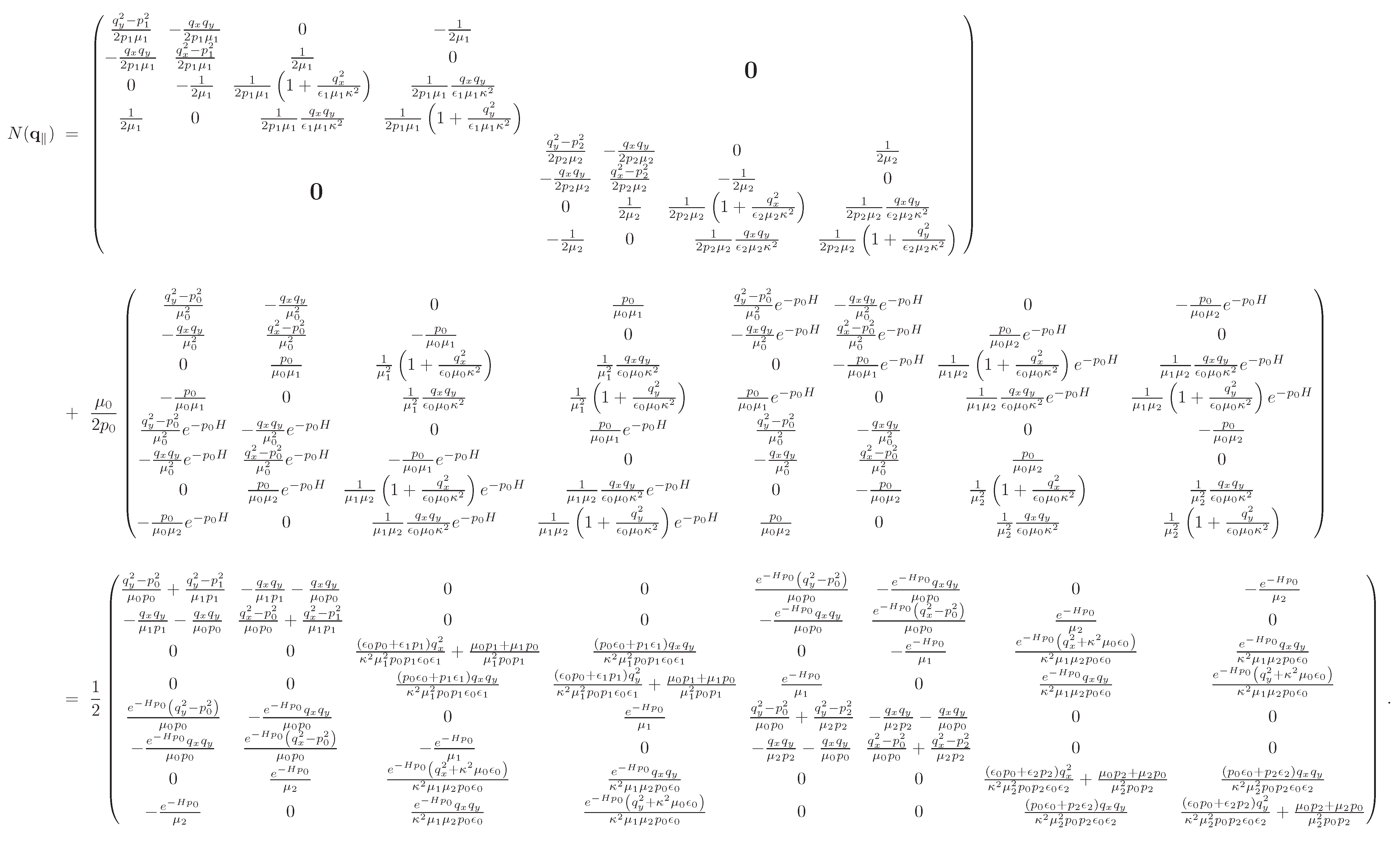
where again the upper (lower) sign everywhere refers to $r=1$ ($r=2$). For the kernel $\widehat{M}$ we determined the sign of the terms $\sim i{q}_z$ from the $q_z$-integration by the observation that z, $z^{\prime }$ have to be taken to the surface with $z-z^{\prime }$ staying outside the object. When combining the kernels $\widehat{L}$ and $\widehat{M}$ into the joint kernel $N_{r{r}^{\prime }}={\widehat{L}}_r{\delta }_{r{r}^{\prime }}+{\widehat{M}}_{r{r}^{\prime }}$, it is diagonal in ${\mathbf{q}}_{\parallel }$-space with the blocks $N\left({\mathbf{q}}_{\parallel }\right)$ on the diagonal given by the $8\times 8$ matrix shown in Figure 2.

The Casimir free energy is given by

$$\mathcal{F}=k_{B}T\sum _{n=0}^{\infty }{}^{\prime }\int \frac{d^2{\mathbf{q}}_{\parallel }}{{\left(2\pi \right)}^2}logdet{\left[N{N}_{\infty }^{-1}\left({\mathbf{q}}_{\parallel }\right)\right]}_{\kappa ={\kappa }_n}$$

(101)

in terms of the determinant of the above matrix where $N_{\infty }$ is the matrix with $H\to \infty$, i.e., the matrix N with the off-diagonal $4\times 4$ blocks $\sim e^{-p_{0}H}$ vanishing. This yields the final result

$$\begin{array}{ccc}\hfill \mathcal{F}& =& k_{B}T\sum _{n=0}^{\infty }{}^{\prime }\int \frac{d^2{\mathbf{q}}_{\parallel }}{{\left(2\pi \right)}^2}log\left[\left(1-\frac{({ϵ}_0{p}_1-{ϵ}_1{p}_0)({ϵ}_0{p}_2-{ϵ}_2{p}_0)}{({ϵ}_0{p}_1+{ϵ}_1{p}_0)({ϵ}_0{p}_2+{ϵ}_2{p}_0)}{e}^{-2p_{0}H}\right)\right.\hfill \\ & \times & \left.\left(1-\frac{({\mu }_0{p}_1-{\mu }_1{p}_0)({\mu }_0{p}_2-{\mu }_2{p}_0)}{({\mu }_0{p}_1+{\mu }_1{p}_0)({\mu }_0{p}_2+{\mu }_2{p}_0)}{e}^{-2p_{0}H}\right)\right],\hfill \end{array}$$

(102)

which is again identical to the Lifshitz formula. Note that in the Hamiltonian approach there is no need to express the kernels in a basis for the space of functions that are regular solutions of the wave equation inside the objects. However, the number of fields per surface is now doubled compared to the Lagrangian approach, resembling the situation in quantum mechanics where the Hamiltonian path integrals run over the canonical coordinates q and p independently.

6. Conclusions

To date, analytical and purely numerical approaches to compute Casimir interactions have been developed independently, and it remained an open question if and how they are related. Analytical methods build on ideas from scattering theory and hence require an expansion of the Green function and bulk or surface operators in terms of special functions that are solutions of the wave equation. Hence, the very existence of such functions and the convergence of the expansion limit these approaches to sufficiently symmetric problems. Purely numerical approaches, such as that developed in [32], can be applied to basically arbitrary geometries but the numerical effort can be extremely high. Hence, it appeared useful to us to study the relation between these approaches in order to develop methods that can serve as semi-numerical approaches that combine the versatility of the purely numerical approaches with the smaller numerical effort of analytical methods. Hence, we have presented in this work a new compact derivation of formulas for the Casimir force, which is based both on bulk and surface operators that also enable analytical evaluations. This we have demonstrated for the simplest case of two dielectric slabs. Further semi-analytical implementations of our approaches are underway.

Our Hamiltonian path integral representation is equivalent to the one derived by Johnson et al. as a purely numerical approach using Lagrange multipliers to enforce the boundary conditions in the path integral. Interestingly, the here-presented derivation of this representation from a Lagrangian path integral demonstrates the relation of this approach to the scattering approach when the T-matrix is defined, as originally by Waterman, by surface integrals of regular solutions of the wave equation over the bodies’ surfaces [38]. This shows the close connection of these approaches, motivating further research in the direction of new semi-analytical methods to compute Casimir forces.

References

- Klimchitskaya, G.L.; Mohideen, U.; Mostepanenko, V.M. The Casimir force between real materials: Experiment and theory. Rev. Mod. Phys. 2009, 81, 1827. [Google Scholar] [CrossRef] [Green Version]
- Rodriguez, A.W.; Hui, P.-C.; Woolf, D.P.; Johnson, S.G.; Lončar, M.; Capasso, F. Classical and fluctuation-induced electromagnetic interactions in micron-scale systems: Designer bonding, antibonding, and Casimir forces. Annalen Physik 2014, 527, 45–80. [Google Scholar] [CrossRef] [Green Version]
- Woods, L.M.; Dalvit, D.A.R.; Tkatchenko, A.; Rodriguez-Lopez, P.; Rodriguez, A.W.; Podgornik, R. Materials perspective on Casimir and van der Waals interactions. Rev. Mod. Phys. 2016, 88, 045003. [Google Scholar] [CrossRef]
- Bimonte, G.; Emig, T.; Kardar, M.; Krüger, M. Nonequilibrium Fluctuational Quantum Electrodynamics: Heat Radiation, Heat Transfer, and Force. Annu. Rev. Condens. Matter Phys. 2017, 8, 119–143. [Google Scholar] [CrossRef] [Green Version]
- Dalvit, D.; Milonni, P.; Roberts, D.; daRosa, F. Casimir Physics; Springer: Berlin/Heidelberg, Germany, 2011. [Google Scholar]
- Golyk, V.A. Non-Equilibrium Fluctuation-Induced Phenomena in Quantum Electrodynamics. Ph.D. Thesis, Massachusetts Institute of Technology, Cambridge, MA, USA, 2014. [Google Scholar]
- Rodriguez, A.W.; Capasso, F.; Johnson, S.J. The Casimir effect in microstructured geometries. Nat. Photonics 2011, 5, 211. [Google Scholar] [CrossRef]
- Emig, T.; Graham, N.; Jaffe, R.L.; Kardar, M. Casimir Forces between Arbitrary Compact Objects. Phys. Rev. Lett. 2007, 99, 170403. [Google Scholar] [CrossRef] [Green Version]
- Maia Neto, P.A.; Lambrecht, A.; Reynaud, S. Casimir energy between a plane and a sphere in electromagnetic vacuum. Phys. Rev. A 2008, 78, 012115. [Google Scholar] [CrossRef] [Green Version]
- Rahi, S.J.; Emig, T.; Graham, N.; Jaffe, R.L.; Kardar, M. Scattering theory approach to electrodynamic Casimir forces. Phys. Rev. D 2009, 80, 085021. [Google Scholar] [CrossRef] [Green Version]
- Krüger, M.; Bimonte, G.; Emig, T.; Kardar, M. Trace formulas for nonequilibrium Casimir interactions, heat radiation, and heat transfer for arbitrary objects. Phys. Rev. B 2012, 86, 115423. [Google Scholar] [CrossRef] [Green Version]
- Emig, T.; Graham, N.; Jaffe, R.L.; Kardar, M. Casimir forces between compact objects: The scalar case. Phys. Rev. D 2008, 77, 025005. [Google Scholar] [CrossRef] [Green Version]
- Kenneth, O.; Klich, I. Opposites attract: A theorem about the Casimir force. Phys. Rev. Lett. 2006, 97, 160401. [Google Scholar] [CrossRef] [PubMed] [Green Version]
- Bimonte, G. Scattering approach to Casimir forces and radiative heat transfer for nanostructured surfaces out of thermal equilibrium. Phys. Rev. A 2009, 80, 042102. [Google Scholar] [CrossRef] [Green Version]
- Bimonte, G.; Emig, T. Exact Results for Classical Casimir Interactions: Dirichlet and Drude Model in the Sphere-Sphere and Sphere-Plane Geometry. Phys. Rev. Lett. 2012, 109, 160403. [Google Scholar] [CrossRef] [Green Version]
- Bimonte, G. Beyond-proximity-force-approximation Casimir force between two spheres at finite temperature. II. Plasma versus Drude modeling, grounded versus isolated spheres. Phys. Rev. D 2018, 98, 105004. [Google Scholar] [CrossRef] [Green Version]
- Kenneth, O.; Klich, I. Casimir forces in a T-operator approach. Phys. Rev. B 2008, 78, 014103. [Google Scholar] [CrossRef] [Green Version]
- Milton, K.A.; Parashar, P.; Wagner, J. Exact Results for Casimir Interactions between Dielectric Bodies: The Weak-Coupling or van der Waals Limit. Phys. Rev. Lett. 2008, 101, 160402. [Google Scholar] [CrossRef] [Green Version]
- Reid, M.T.H.; Rodriguez, A.W.; White, J.; Johnson, S.G. Efficient Computation of Casimir Interactions between Arbitrary 3D Objects. Phys. Rev. Lett. 2009, 103, 040401. [Google Scholar] [CrossRef]
- Golestanian, R. Casimir-Lifshitz interaction between dielectrics of arbitrary geometry: A dielectric contrast perturbation theory. Phys. Rev. A 2009, 80, 012519. [Google Scholar] [CrossRef] [Green Version]
- Ttira, C.C.; Fosco, C.D.; Losada, E.L. Non-superposition effects in the Dirichlet–Casimir effect. J. Phys. A 2010, 43, 235402. [Google Scholar] [CrossRef] [Green Version]
- Hartmann, M.; Ingold, G.-L.; Neto, P.A.M. Plasma versus Drude Modeling of the Casimir Force: Beyond the Proximity Force Approximation. Phys. Rev. Lett. 2017, 119, 043901. [Google Scholar] [CrossRef]
- Bordag, M.; Robaschik, D.; Wieczorek, E. Quantum field theoretic treatment of the Casimir effect. Ann. Phys. 1985, 165, 192. [Google Scholar] [CrossRef]
- Bordag, M. Casimir effect for a sphere and a cylinder in front of a plane and corrections to the proximity force theorem. Phys. Rev. D 2006, 73, 125018. [Google Scholar] [CrossRef] [Green Version]
- Emig, T.; Hanke, A.; Golestanian, R.; Kardar, M. Normal and lateral Casimir forces between deformed plates. Phys. Rev. A 2003, 67, 022114. [Google Scholar] [CrossRef] [Green Version]
- Büscher, R.; Emig, T. Towards a theory of molecular forces between deformed media. Nucl. Phys. B 2004, 696, 468. [Google Scholar]
- Teo, L. Material dependence of Casimir interaction between a sphere and a plate: First analytic correction beyond proximity force approximation. Phys. Rev. D 2013, 88, 045019. [Google Scholar] [CrossRef] [Green Version]
- Huth, O.; Rüting, F.; Biehs, S.; Holthaus, M. Shape-dependence of near-field heat transfer between a spheroidal nanoparticle and a flat surface. Eur. Phys. J. Appl. Phys. 2010, 50, 10603. [Google Scholar] [CrossRef] [Green Version]
- Incardone, R.; Emig, T.; Krüger, M. Heat transfer between anisotropic nanoparticles: Enhancement and switching. Europhys. Lett. 2014, 106, 41001. [Google Scholar] [CrossRef] [Green Version]
- Graham, N.; Shpunt, A.; Emig, T.; Rahi, S.J.; Jaffe, J.L.; Kardar, M. Electromagnetic Casimir forces of parabolic cylinder and knife-edge geometries. Phys. Rev. D 2011, 83, 125007. [Google Scholar] [CrossRef] [Green Version]
- Emig, T.; Graham, N. Electromagnetic Casimir energy of a disk opposite a plane. Phys. Rev. A 2016, 94, 032509. [Google Scholar] [CrossRef] [Green Version]
- Reid, H.M.T.; White, J.; Johnson, S.G. Fluctuating surface currents: An algorithm for efficient prediction of Casimir interactions among arbitrary materials in arbitrary geometries. Phys. Rev. A 2013, 88, 022514. [Google Scholar] [CrossRef] [Green Version]
- Harrington, R.F. Time-Harmonic Electromagnetic Fields; Wyley: New York, NY, USA, 2001. [Google Scholar]
- Lifshitz, E.M.; Pitaevskii, L.P. Statistical Physics: Part 2; Pergamon: Oxford, UK, 1980. [Google Scholar]
- Agarwal, G.S. Quantum electrodynamics in the presence of dielectrics and conductors. I. Electromagnetic field response functions and black-body fluctuations in finite geometries. Phys. Rev. A 1975, 11, 230–242. [Google Scholar] [CrossRef]
- Rytov, S.M.; Kravtsov, Y.A.; Tatarskii, V.I. Principles of Statistical Radiophysics; Springer: Berlin, Germany, 1989. [Google Scholar]
- Lifshitz, E.M. The theory of molecular attractive forces between solids. Sov. Phys. JETP 1956, 2, 73. [Google Scholar]
- Waterman, P.C. Symmetry, Unitarity, and Geometry in Electromagnetic Scattering. Phys. Rev. D 1971, 3, 825. [Google Scholar] [CrossRef]
- Landau, L.D.; Lifshitz, E.M. Electrodynamics of Continuous Media; Pergamon: Oxford, UK, 1984. [Google Scholar]
- Eckhardt, W. Macroscopic theory of electromagnetic fluctuations and stationary heat transfer. Phys. Rev. A 1984, 29, 1991–2003. [Google Scholar] [CrossRef]
- Harrington, R.F. Boundary integral formulations for homogeneous material bodies. J. Electr. Wav. Appl. 1989, 3, 1–15. [Google Scholar] [CrossRef]
Figure 1.
Configuration of bodies: (a) general shapes and positions that can be studied with the approaches presented in this work, (b) non-penetrating configurations that can be studied within the scattering approach.
Figure 2.
Matrix forming the diagonal blocks of the matrix N.
Publisher’s Note: MDPI stays neutral with regard to jurisdictional claims in published maps and institutional affiliations. |
© 2021 by the authors. Licensee MDPI, Basel, Switzerland. This article is an open access article distributed under the terms and conditions of the Creative Commons Attribution (CC BY) license (https://creativecommons.org/licenses/by/4.0/).
Share and Cite
MDPI and ACS Style
Bimonte, G.; Emig, T. Unifying Theory for Casimir Forces: Bulk and Surface Formulations. Universe 2021, 7, 225. https://0-doi-org.brum.beds.ac.uk/10.3390/universe7070225
AMA Style
Bimonte G, Emig T. Unifying Theory for Casimir Forces: Bulk and Surface Formulations. Universe. 2021; 7(7):225. https://0-doi-org.brum.beds.ac.uk/10.3390/universe7070225
Chicago/Turabian StyleBimonte, Giuseppe, and Thorsten Emig. 2021. "Unifying Theory for Casimir Forces: Bulk and Surface Formulations" Universe 7, no. 7: 225. https://0-doi-org.brum.beds.ac.uk/10.3390/universe7070225
Note that from the first issue of 2016, this journal uses article numbers instead of page numbers. See further details here.