
Relativistic Cosmology with an Introduction to Inflation


1
Department of Mathematics, University of Gujrat, Gujrat 50700, Pakistan
2
Department of Applied Mathematics and Statistics, Technical University of Cartagena, 30310 Cartagena, Spain
3
Department of Mathematics, Faculty of Science, King Abdulaziz University, P.O. Box 80203, Jeddah 21589, Saudi Arabia
*
Author to whom correspondence should be addressed.
Universe 2021, 7(8), 276; https://0-doi-org.brum.beds.ac.uk/10.3390/universe7080276
Submission received: 23 June 2021
/
Revised: 20 July 2021
/
Accepted: 26 July 2021
/
Published: 30 July 2021
Abstract
:In this review article, the study of the development of relativistic cosmology and the introduction of inflation in it as an exponentially expanding early phase of the universe is carried out. We study the properties of the standard cosmological model developed in the framework of relativistic cosmology and the geometric structure of spacetime connected coherently with it. The geometric properties of space and spacetime ingrained into the standard model of cosmology are investigated in addition. The big bang model of the beginning of the universe is based on the standard model which succumbed to failure in explaining the flatness and the large-scale homogeneity of the universe as demonstrated by observational evidence. These cosmological problems were resolved by introducing a brief acceleratedly expanding phase in the very early universe known as inflation. The cosmic inflation by setting the initial conditions of the standard big bang model resolves these problems of the theory. We discuss how the inflationary paradigm solves these problems by proposing the fast expansion period in the early universe. Further inflation and dark energy in modified gravity are also reviewed.
1. Introduction
With the advent of general relativity in 1916, spacetime transformed itself into one of the four fundamental interactions of the universe and the geometrical structure attached to it was taken to demonstrate gravity in a dynamical way [1]. The force of gravity was replaced by the curvature of spacetime that is mirrored through the geometric structure of metric tensor . The spacetime became an integral part of the universe and a dynamical medium where the whole phenomenal universe exists. Any solution of the field equations of general relativity entails a certain structural geometry of spacetime or just a spacetime that represents a universe itself, therefore determining a solution of the field equations is similar to coming across a specific model of the universe.
Cosmology studies the universe as a whole [2] encompassing its beginning in spacetime or as spacetime itself, its evolution, and its eventual ultimate fate. The history of cosmology dates back to ancient Greeks, Indians, and Iranians with its roots at that time in philosophy and religion. Before modern scientific cosmology emerges, it has been nurtured in the womb of Ibrahamic religions especially Judaism, Christianity, and Islam. Cosmology as modern science begins with the surfacing of general relativity when Einstein first himself put it to use to formulate a cosmological model of the universe mathematically. The model brought about a dynamic universe but was rendered to be static as there was no cosmological evidence of its contraction or expansion at that time [3]. Einstein’s static model was afterward proved to be inconsistent with cosmological observations and was discarded; however, its formulation as the first mathematical model based on the field equations of general relativity laid the foundational stone for the inception of modern relativistic cosmology as science.
Cosmology takes into account the largest scale of spacetime that is the causally connected maximal patch of the cosmos from the perspective of its origin, evolution, and futuristic eventual fate. It gives the universe a mathematical description as large as the cosmological observational parameters reveal and allow consequently. The modern relativistic cosmology was established on general relativity which brought forth the big bang model of the universe. The big bang model was marred with some inward problems related to it, which were removed by introducing an exponentially expanding phase in the early universe known as inflation. de Sitter presented a model of the universe devoid of ordinary matter, however with the cosmological constant term retained. The geometry of the model was proved to be accelerating [4]. The de Sitter universe corresponds to the specific case related to one of the very early solutions of Einstein’s Field Equations (EFE). The importance of the de Sitter model was not recognized until the introduction of inflation in the late 20th century, as the actual universe must be considered as a local set of perturbations in the geometry of de Sitter having validity at large. de Sitter geometry represents Euclidean space with a metric that depends on time. It was found that the inflation could be the de Sitter in general or quasi-de Sitter geometry which has an innate impact on the evolution of the geometry of FLRW spacetimes. It further bears its relation with the late-time accelerated expansion of the universe and to the dynamic geometry of the spacetime intrinsically cohered with it. The paradigm of inflation, as it is propounded, has a profound impact on the evolution of the universe as the geometry of spacetime. The de Sitter universe represents the inflationary phase of the universe with slightly broken time translational symmetry.
Alexander Friedmann predicted theoretically the universe to be dynamic, the one which can expand, contract, or even be born out of a singularity [5]. George Lemaitre, unaware of Friedmann’s work at that time, independently reached the same conclusion. In 1931, he also proposed a theory of the primeval atom which came to be known later on as the big bang theory by Fred Hoyle accidentally [6]. Edwin Hubble first proved the existence of other galaxies besides the Milky Way and afterward in 1929 discovered based on observational evidence that the universe is actually expanding [7]. This was actually discovering what Friedmann already had predicted theoretically in 1922. In the late 1940s, George Gamow (1904–1968) and his collaborators, Ralph Alpher (1921–2007) and Robert Herman (1914–1997), independently worked on Lemaître’s hypothesis and transformed it into a model of the early universe. They made supposition about the initial state of the universe comprising of a very hot, compressed mixture of nucleons and photons, thereby introducing the big bang model on the basis of comparatively strong evidences. They did not associate a particular name with the early state of the universe. Based on this model they were successful in calculating the amount of helium in the universe, but unfortunately, there was no authentic observational evidence through which their calculations could be compared [8].
The standard relativistic model of cosmology underpinning big bang theory could not explain the global structure of the universe and the origin of matter in it. The distribution of matter in it homogeneously on large scales and the spatial flatness also remained enigmatic. The big bang model just made an assumption about these but could not solve them. In the framework of effective field theory, the aspects of nonsingular cosmology were explored by Yong Cai et al. It is shown that the effective field theory assists in having the clarification about the origin of no-go-theorem and helps to resolve this theorem [9].
The inflationary era was proposed in the standard model of cosmology which propounds the big bang theory of the creation of the universe. Inflation solves the problems encountered in the big bang cosmology. Gliner, in 1965, hypothesized an era of exponential expansion for the universe earlier than any significant inflationary model surfaced [10]. It was found that the scalar fields are dynamic in nature, and in 1972 it was proposed that during phase transitions the energy density of the universe as a scalar field changes [11]. Andrei Linde, in 1974, realized that scalar fields can play an important role in describing the phases of the very early universe. He speculated that the energy density of a scalar field can play the role of vacuum energy dubbed as a cosmological constant [12].
In 1978, Englert, Brout, and Gunzig [13] forwarded a proposal of “fireball” hypothesis attempting to resolve the primordial singularity problem. They based their investigations on the entropy contained in the universe and approached the issue of early evolution of the universe by introducing particle production in it. They inquired deep down into it and on the basis of their hypothesis inferred that a universe undergoing a quantum mechanical effect would itself appear in a state of negative pressure and would be subject to a phase of exponential expansion. A work was mentioned by Linde in his review article [14] where he sought, in collaboration with Chibisov, to develop a cosmological model based upon the facts known in connection with the scalar fields. Considering the supercooled vacuum as a self-contained source for entropy, they tried to bring about the exponential expansion of the universe to be concerned with it. They, however discovered instantly that the universe becomes very inhomogeneous after the bubble wall collisions take place.
Slightly before Alan Guth’s original proposal of inflation surfaced, Alexei Starobinsky in 1980 proposed a model of inflation on the base of a conformal anomaly in quantum gravity. His proposal was presented in the framework of general relativity where slight modification of the equations of general relativity in matter sector was proposed and quantum corrections were employed to it in order to have a phase of the early universe. Starobinsky’s model can be considered as the first model of inflation which is of semi-realistic nature and evades from the graceful exit problem [15]. It was hardly concerned with the problems of homogeneity and isotropy which occur in the relativistic cosmological model of the big bang. His model, as he himself accentuated, can be considered the extreme opposite of chaos in Misner’s model. The model is found to agree with cosmological observations with slight deviations form recent measurements. Tensor perturbations that represent gravitational waves have also been predicted in Starobinsky’s model with a spectrum that is flat.
Alan Guth employed the dynamics of a scalar field and with a clear physical motivation presented an inflationary model [16] in 1981 on the base of supercooling theory during the cosmic phase transitions where the universe expands in a supercooled false vacuum state. A false vacuum is a metastable state containing a huge energy density without any field or particle so that when the universe expands from this heavy nothingness state its energy density does not change and empty space remains empty so that the inflation occurs in false vacuum [17]. The duration of inflationary phase in Guth’s original scenario is too short to resolve any problem, although was supposed to solve these problems and consequently the universe becomes very inhomogeneous which leads to the graceful exit problem [18,19]. The problem prevents the universe from evolving to later stages and is inherently existing in the originally proposed version of Guth.
The graceful exit problem was addressed independently by Linde, Steinhard, and Albrecht [20,21,22,23,24,25], where they introduced a phase of slow roll inflation at the end of the normal inflationary phase inclusively known as new inflation. The resolution of the problem was sought by constructing a new inflationary paradigm where the inflation can have its inception either in an unstable state at the top of the effective potential or in the state of false vacuum. In this scenario, the dynamics of the scalar field is such that it rolls gradually down to the lowest of its effective potential. It is of great importance to note that the shifting away of the scalar field from the false vacuum state to other later states has remarkable consequences. When the scalar field rolls slowly towards its lowest so-called slow roll inflation, the density perturbations are generated which seed the structure formation of the universe [26,27,28]. The production of density perturbations during the phase of slow roll inflation is inversely proportional to the motion of the scalar field [29,30]. The basic difference between the new inflationary scenario and that of the old one is that the advantageous portion of the inflation in the new scenario, which is responsible for the large scale homogeneity of the universe, does not take place in the false vacuum state, where the scalar field vanishes. This means that the new inflation could explain why our universe was so large only if it was very large initially and contained many particles from the very beginning.
The course of 20th century has presented many challenges to the standard cosmology. In the framework of the standard model, in addition to inflation, another breakthrough came forth in 1998 when the observation-based accelerated expansion of the universe was discovered [31,32,33]. Before this discovery, however, it was thought that in the perspective of all known forms of matter and energy that obey the strong energy condition , the expansion of the universe would slow down with the passage of time. This was a natural consequence of Friedmann equations that play a central role in the evolution of the universe. From the acceleration equation , the universe must be undergoing deceleration characterized by deceleration parameter ; however, astoundingly the value of was observationally determined, meaning that the expansion of the universe is accelerating rather to be decelerating. The discovery of accelerated expansion has won Noble prize in 2011. To explain the cause of accelerated expansion an exotic form of energy density was introduced hypothetically known usually as dark energy. The present budget of the universe from the observational data is contributed by dark energy , dark matter and ordinary baryon matter [34,35]. Dark energy is effective on the largest scales of intra galaxies and does not affect gravitationally bound systems. To explain the origin of dark energy, there is a large number of proposed models. Many independent observations lend support to the existence of dark energy such as CMB, SN Ia, BAO, etc. Today dark energy constitutes a very significant subject of relativistic cosmology with observational data by providing information about its basic nature, for reviews see in [36,37,38]. In this article, we study the standard model of cosmology by investigating the geometric structure of spacetime related with it in the framework of general relativity. Beginning with Euclidean space, we study spacetime in special and general theory of relativity. We discuss problems encountered in the standard big bang cosmology, and the inflationary solutions introduced into it, by proposing a phase of accelerated expansion in the early universe. A discussion of modified gravity is also presented with discussion of how inflation and dark energy can be described in its framework.
The layout of the paper is as follows. In Section 2, we discuss the structure of Euclidean space beginning with the axioms of Euclidean geometry and the significant role played by the Pythagoras theorem in its development. It has four subsections discussing space, time, and spacetime in relativity and pre-relativity physics. Section 3 begins with relativistic cosmology with a discussion on its underlying principles. The standard model of cosmology is discussed in Section 4 with nine subsections about its geometric structure. In Section 5, the derivation of Friedmann equations is carried out. Section 6 describes different aspects of embedding a geometrical object in a space of higher dimensions. It is has four subsections. Section 7 presents the very first relativistic model developed by Einstein himself. It has two subsections that discuss the instability of Einstein’s universe and de Sitter’s empty universe model respectively. In Section 8, a discussion on conformal FLRW line elements is presented in addition to the vacuum, radiation, and matter-dominated eras. It has 12 subsections covering related topics. Section 9 with its four subsections is devoted to the discussion of cosmological problems faced by the standard model. In Section 10, we embark on inflation and discuss its dynamics. Section 11 describes how the proposal of exponential expansion in the early universe solves the cosmological problems. CDM and are discussed in this section. In the last Section, we provide a summary of the paper. Four indices are added in the end.
2. Euclidean Space
Euclidean geometry is established on a set of simple axioms and the definitions derived from these axioms. These axioms were first stated by Euclid in about 300 B.C. [39]. A space at the level of mathematical abstraction is the set of points where each point represents a specific position in it. When an abstract space is mapped onto a physical space, each point of it represents a physical location in it. Euclidean space is what entails on the base of axioms of Euclidean geometry. Geometrically, a space can be described by reducing it to a certain specification of the distance between each pair of its neighboring points. In order to reduce all of the geometry of a space to a certain specification of the distance between each pair of neighboring points we use the metric or line element which measures the space and describes its nature. A line element specifies a certain geometry and its form varies corresponding to different coordinate systems. Five basic postulate lie at the core of Euclidean space and are the basis of standard laws of geometry:
- 1.
- Any two points can be joined by a straight line, i.e., the shortest distance between two points is a straight line.
- 2.
- A straight line can be extended to any length.
- 3.
- A circle can be drawn with a given a line segment as radius and one end as center of the circle.
- 4.
- All right angles are congruent.
- 5.
- Given a line and a point not on the line, it is possible to draw exactly one line through the given point parallel to the line, i.e., parallel lines remain a constant distance apart. Pythagoras theorem was known before Euclid and can also be derived from the five postulates and is used to find distance between any two points in Euclidean space. A mathematical space is an abstraction used to model the physical space of the universe. The Euclidean space consists of geometric points and has three dimensions. Now the Pythagorean theorem for a right triangle describes how to calculate the length of hypotenuse when the lengths of other two sides namely base and altitude are given. The length of hypotenuse gives distance between two points. Figure 1 below shows Pythagoras theorem:
Now, as the space can be described everywhere consisting of geometric points, we can define mutual relation for every infinitesimally close three points of the space forming a right triangle so that we can determine the element of distance between any two points with the help of Pythagoras theorem. Using rectangular Cartesian coordinate system we can express distance between two points in differential form as
The distance-measure by Pythagoras theorem in Equation (2) will be known as metric or line element in two dimensions and defines Euclidean metric for two dimensional space. The distance measured between two points by the metric in Equation (2) does not change on rotating the coordinate system in which these two points are specified as Figure 2 manifests it:
or
The distance between two points remains invariant which means that
The Pythagorean theorem in three dimensions can be described as
Three mutually perpendicular planes along three dimensions of the Cartesian coordinate system divide it in 3-planes as is shown in Figure 3:
Now, in reference to a coordinate system each point of this space will have three coordinates if we approach its structure through Cartesian scheme, i.e., in Cartesian coordinates each point of it is represented by three coordinates which are the distances measured starting from the origin of the coordinate axes along the corresponding axes, i.e., x-axis, y-axis, and z-axis, respectively. These three axes stand for three dimensions of space. We find the distance between two points with Cartesian coordinate for three points separated infinitesimally
which gives the metric of three-dimensional space The distance between two points with Cartesian coordinates and will be
The infinitesimal distance between any two points and can be had using the metric written above in Equation (7) in three dimensional Euclidean space.
or in tensor form
where is the Kronecker delta function representing a symmetric tensor of rank two and can be expressed as a matrix form
diagonal of
and trace of
therefore, in Equation (13) defines an n-dimensional Euclidean space.
Equation (21) can also be written in the form
From Equation (22), we can see that the inner product in three dimensional Euclidean space can be perfectly described, that is why three dimensional Euclidean space is an example of a complete inner product space. An explanatory discussion of maximally symmetric 3 space can be consulted in Appendix B.
2.1. Newtonian Mechanics: The Structure of Space and Time
Space and time are absolute structures in classical physics and can be distinguished from one another in an independent way. Newton’s Mechanics is based specifically on three laws of motion, a law of gravitation and Galilean principle of relativity which are inherently related with the properties of space and time. Newtonian space is a three-dimensional extension around us which constitutes absolute space. Absolute space in Newton’s own words is described as “Absolute space, in its own nature, without relation to anything external remains always similar and immovable”, therefore space is rigid, motionless, and can be viewed as colossally empty three-dimensional cubic or cuboidal box where material objects reside and all physical phenomena take place. Newtonian space has the properties of Euclidean pace where infinitesimal distance between any two points is a straight line and if three points constitute a right angled triangle, then three sides are related by Pythagoras theorem which ascribes to it the properties of a flat space. Sum of angles in a triangle in such space is . Newtonian space is homogeneous and isotropic which entails Newtonian Mechanics. Homogeneity implies translational invariance of the properties of space which means that it has similar properties at every point contained in it. The property of being homogeneous is called homogeneity that leads to the invariance of physical laws performed in two or more coordinate systems. Newton’s 3rd law, law of conservation of momentum and energy, etc. come out as a consequence of homogeneity of space. It is also an isotropic that implies rotational invariance of the properties of space. It means that it has similar properties in all directions and is therefore direction-independent. Thus, isotropy implies homogeneity but the converse is not true. The absolute time has been enunciated as follows “Absolute time, and mathematical time of itself and from its own nature flows equably without relation to anything external, and is otherwise called duration” such time exists independent of space and whatever dynamically happens in it and flows uniformly in one direction. An interval of time possesses always unchanging meaning for all times. This is presented figuratively in Figure 4 below:
According to Newtonian Mechanics, gravitation and relative motion do not affect the rate at which time flows. From Newton’s 2nd law , the isotropy of time can be viewed in case of a dynamic system that does not change from perpetrating transition from to . This is because it does not incorporate the element of time explicitly which implies that past and future are indistinguishable but this is paradoxical because time is unidirectional and flows always from past to future. Two observers in two inertial frames of reference in relative motion and equipped with standard measuring clocks record the spacetime coordinates of an event written as and , respectively. According to Galilean principle of relativity, the coordinate transformations are
We can calculate the addition of velocities according to these transformations by differentiating the spatial parts of Equation (23) with respect to time t, we have
As , we infer that . Likewise, acceleration can also be differentiated once again from Equation (24), which gives
We can observe from Equation (25) that the accelerations in both frames are same. The time-coordinate of one inertial frame remains unaffected during transformation to another inertial frame of reference in classical physics and does not depend on spatial coordinates x, y, and z. The set of equations in Equation (23) are known as Galilean transformations. The motion along y and z spatial dimensions remains unaffected and the time coordinates in the two frames are equivalent which implies that time is absolute as Newton believed meaning that for all the inertial observers the time interval between any two events would be invariant. We notice that the two events having coordinates and , respectively, with differential of the distance as Euclidean spatial interval described in Equation (21) as and the time interval both remain separately invariant under the Galilean transformations in Equation (23). This fact makes us consider the nature of space and time as absolute entities in Newtonian Mechanics. We identify the quantity as square of the distance between points of three-dimensional Euclidean space and invariance of this differential of distance alludes to the fact that it is geometrical structural property of the space itself in its own right. This describes the geometry of space and time according to Newton’s views.
2.2. Special Theory of Relativity: The Structure of Spacetime
Special relativity is a theory of the structure of spacetime and in this way constitutes a geometric theory [40]. The fields and particles grow over this spacetime structure and relativistic mechanics is developed according to this structure which corresponds to the postulates of special relativity. According to the Lorentz transformations implied by it, space and time are not distinguishable quantities but constitute innately a single continuum to be known as spacetime. One of the Einstein’s 1905 papers brought forward this theory founded upon two postulates [41].
- 1.
- The principle of special covariance.
- 2.
- The principle of invariance of the velocity of light (c). As the laws of physics remain form-invariant, i.e., covariant according to a privileged class of observers known as inertial frames. This is also called principle of relativity. These two principles overthrew the pre-relativity notions of absolute space and absolute time proposing instead relative concepts. In classical physics as we saw earlier the coordinates of two observers are related by Galilean transformations, whereas according to the special relativity, the coordinates in two frames are related using Lorentz transformations.Lorentz transformations contain all the geometric information about space and time, and describe the structure of spacetime. Further, we can see that space and time coordinates are absolute according to the Galilean transformations for two inertial observers which move relative to each other and are connected through space and time coordinates. Time coordinate has the same magnitude in pre-relativity physics; however, according to the special relativity, which obeys Lorentz transformations, the time coordinate in one coordinate system is connected to the time coordinate of the second coordinate system through both time and space coordinates, which alludes to the fact that space and time coordinates are now to be dealt on equal footings. It is obvious from the Lorentz transformations that the time coordinates are not equivalent in two frames, i.e., rather is innately cohered with both of the coordinates of time and space t and x respectively. It means that time of one coordinate frame converts partially in space and partially in time coordinates. Therefore, does not remain independent but has partially coalesced with space coordinates losing its absolute nature and the principle of relativity forbade us to locate a preferred frame of reference ensuing that absolute notion of time disappears logically. This fact was first perceived by Minkowski when he was recasting the special relativity in the language of geometry. He has presented a very profound and significant geometrical structure underlying special relativity. While delivering a lecture at the meeting of the Göttingen Mathematical Society on 5 November 1907, he introduced the concept of spacetime continuum whereby he asserted that independent space and time have to doom away into mere shadows and only a union of the two can preserve an independent reality. Minkowski viewed that the principle of special relativity can be described by the metric on the four-dimensional space which familiarized the concept of spacetime continuum and paved the way for the formulation of general relativity. A Minkowski metric g on the linear space is a symmetric non-degenerate bilinear form with signature . It means that there exists a basis such that where and is expressed in the formso that an we have orthonormal basis and can construct a system of coordinates of as such that at each point we can have and where . Now, with respect to this coordinate system, we can write the metric tensor in the form or The negative sign with one time component term in the metric indicates that it is not Euclidean space but represents a pseudo-Euclidean known as Minkowski space and also guarantees that the speed of light is same in all inertial frames. An expanding Minkowskian spacetime can be described in the form as written below which represents the simplest of all dynamic spacetimes . It was thought convenient on the dimensional grounds to introduce the coordinates in the form . Pythagoras theorem applied in Euclidean space of three spatial dimensions gives the distance of two points as an invariant as we observed in previous section.here the length element is a scalar quantity which means that in certain frame of references all the observers will agree upon the length of the measured object. In 1905, Einstein speculated that the measurement of the spacetime intervalwherewould not result in identical either in space or in time [42] for the observers in relative uniform motion. However, Minkowski noted that the four-dimensional entity in Equation (29) would remain invariant for all such observers. The basic significant idea which Minkowski took notice of was that the spacetime interval remains invariant for all the observers in uniform relative motion meaning that it is also a scalar upon which they all will agree. The metric of Minkowski space which is homogenous and isotropic is given bythus the geometry of spacetime is flat in special relativity. It is notable here that it is spacetime that is flat, however in classical mechanics, it is space rather than spacetime. If the Minkowskian geometry of spacetime is required to be expanding, it can be made so. However, in the framework of special relativity, it does not need to expand. Figure 5 gives the structure of Minkowskian spacetime as a null cone structure. In the Figure 6, it is shown how the dimension time is converted in as space.
2.3. General Theory of Relativity: The Structure of Spacetime
The essence of general relativity is that geometry is gravity which comes from Equivalence principle. It models gravity into the dynamic structure of spacetime. In general relativity, the structure of spacetime is described by a fundamental quantity called the spacetime metric or line element which gives the nature of the geometry of spacetime by finding the distance between two infinitesimally neighboring points in it. The geometrical structure of spacetime is incarnated [43] in two basic principles.
- 1.
- Principle of general covariance.
- 2.
- The spacetime continuum has, at each of its points, a quadratic structure of coordinate differentials known as “square of the interval” between the two points under consideration.
We consider a four-dimensional continuum every point of which is distinct from the other with four coordinates-a quadruplet assigned consecutively to each of them
It is denoted by . In matrix form with components, it is written as
The properties of spacetime that are intrinsically related to it, are completely determined by the spacetime metric. An example of the local curved spacetime around the Sun in two dimensions is displayed in Figure 7:
A detailed discussion of space, time and spacetime is presented in Appendix A.
2.4. The Basics of General Relativity
It would be convenient to have a retrospective look into the basics of general relativity whose role has been very fundamental to the modern cosmology. We briefly review the structure of the theory specifically in connection with the geometrical structure of spacetime in it. General relativity in its core describes that gravity is the geometry of four-dimensional spacetime manifested through its curvature. It is a theory of spacetime and gravitation that are the very basic components of the universe. Einstein’s journey towards general relativity in order to introduce gravity in his previous theory sought the fascinating geometry of the structure of spacetime, such that gravity as a field force disappeared and was assimilated in the very geometric structure of spacetime. In constructing the framework of new theory, Einstein was influenced and governed by Mach’s principle, which states that it is a priori existence and distribution of matter which determines the geometry of spacetime, and in the absence of it, there shall be no geometric structure of a spacetime in the universe. Therefore, there will be no inertial properties in an, otherwise, empty universe. In general, relativity gravitation and inertia are essentially indistinguishable. The metric tensor describes the effect of both combinedly, and it is arbitrary to ask which one contributes its effect more and which less, therefore to call it with a single name is suitable either inertia or gravitation [4]. In general relativity gravitation, inertia and the geometry of spacetime are coalesced into a single entity represented by a symmetric tensor of second rank which owes its existence due to presence and distribution of matter which is represented by an other symmetric tensor known as energy-momentum tensor. The metric tensor is the fundamental object of study in general relativity and takes into consideration all the causal and geometrical structure of spacetime. General relativity underlies five fundamental principles connotated by it implicitly or explicitly manner:
- Mach’s principle
- principle of equivalence
- principle of covariance
- principle of minimal gravitational coupling
- correspondence principle
In the light of the principle of general covariance, the theory requires that the laws of physics might be formulated in a coordinate-independent style. The coordinate independence requires the replacement of partial derivatives by covariant derivatives which introduces connection coefficients as the 2nd kind of Christoffel symbols. All the geometric structure of spacetime is based on the existence of these connection coefficients. The field equations of general relativity read as , where is the Einstein tensor and is expressed in terms of Ricci tensor, metric tensor, and Ricci scalar, and is energy momentum tensor. The spacetime continuum of general relativity is postulated as a 4-dimensional Lorentzian manifold (M, g), where M denotes the Manifold and g is metric defined over it. The geometry of a spacetime is encoded in its metric which has a geodesic structure, though complex and frequently solved numerically for a specific bunch of geodesics. These geodesics specify the physical properties of the geometry of spacetime which are interpreted by drawing graphically in a certain spacelike volume. Gravity is the geometry of spacetime itself which is described through its dynamic structure in the framework of general relativity. The interaction between spacetime and the content it contains which mutually form and the universe is the pith and marrow of general relativity. Matter tells spacetime how to curve and spacetime tells the matter how to move. General relativity thus transforms gravitation from being a force to being it a property of spacetime, so that gravity does remain a force but curvature of the geometric structure of spacetime. Einstein worked out a relation between matter–energy content of the universe and its gravitating effects in the form of geometry of spacetime. He employed the language of tensors to describe it. The invariant interval between two events separated infinitesimally with coordinates and has been defined according to special relativity
Which defines a Lorentz invariant Minkowski flat spacetime whose geometry of spacetime is encoded in . Under the change of coordinates remains invariant and is spacelike for , timelike for and light-like for . Photon path is described by and baryonic matter follows a path between two events for which
i.e., it generates stationary values and conforms to the shortest distance between two points to be straight line which means that there are no external forces to set their path deviated. General relativity was based on five principles incorporated in it explicitly or implicitly, namely, equivalence principle, relativity principle, Mach’s principle, and Correspondence principle. Tensors are geometric objects defined on a manifold M, which remain invariant under the change of coordinates. It is composed of a set of quantities which are called its components, therefore a it is the generalization of a vector which means that it has more than three components. They represent mathematical entities which conform to certain laws of transformations. The properties of components of a tensor do not depend on a coordinate system which is used to describe the tensors. Transformation laws of a tensor relate its components in two different coordinate systems. The mathematical representation of a tensor is displayed through considering usually a bold face alphabetical letter like A, B, T, P, etc. with an index or a set of indices in the form of superscripts or subscripts or both in mixed form. These superscripts and subscripts in case of a tensor are called contravariant and covariant indices. Contravariant indices of a tensor are used to give the meaning of a contravariant components of it like , , . Covariant indices of a tensor are used to signify the meaning of a contravariant components of it like , , . The indices of both types namely contravariant and covariant are used to specify the components of a mixed tensor like , , , . A mixed tensor is a tensor which has contravariant as well as covariant components. The number of indices appearing in the symbol representing certain type of a tensor is known as its rank. The appearing indices in the symbol representing a tensor can be contravariant or covariant or both type of indices in it. The order of a tensor is the same thing as rank, only the name differs. The number of components of a tensor is related with its rank or order and the dimensions of the space in which the is being described. In an n-dimensional space, a tensor of rank, say, k will have number of components equal to number of components of a tensor in n-dimensional space is equivalent to . However, the spacetime of general relativity is pseudo-Riemannian having four dimensions, three spatial and one temporal. Coordinate patches are necessarily considered to map whole of the spacetime. Each point-event of a coordinate patch in the four-dimensional pseudo-Riemannian spacetime is labeled by a general coordinate system, which conventionally runs over 0, 1, 2, and 3, where 0 stands for time and the rest for space coordinates. An inertial or otherwise frame of reference characterized by a coordinate system can be attached to every point event of the spacetime and coordinate transformations between any two coordinate systems can be found. These can be written as
while switching to Riemannian geometry for non-Euclidean spaces ordinary partial differentiation is generalized to covariant differentiation and is defined using a semi-colon; as
where comma, denotes an ordinary partial differentiation with respect to the corresponding variable and; signifies covariant differentiation. In the covariant differentiation, indices can also be raised or lowered with metric tensor, however the covariant differentiation of it vanishes, i.e., . The interval between infinitesimally separated events and is given by
The corresponding contravariant tensor of is given by and they result in Kronecker delta. Moreover, indices can be lowered or raised using the metric tensor in either form as
In general relativity, all the geometry of curved spacetime is contained in the second-rank symmetric tensor known as fundamental or metric tensor and is the function of four coordinates and encodes all the information about gravitational field induced by presence of matter. It governs the other matter as a response mimicking the role of gravitational potential similar to that of Newtonian gravity so that the paths remain no more straight, and the action in Equation (36) determines the path of a free particle known as geodesic
where
are the Christoffel symbols which through the geodesic equation specify the world lines of free particles. The “acceleration due to gravity” in Newtonian gravitation law is described by these symbols in Einstein’s picture of gravity as the geometric properties of spacetime encoding the similar information. Locally these symbols vanish in the inertial frame of reference in free fall and under coordinate transformation from and do not constitute components of a tensor and therefore do not represent a tensor.
The Riemann tensor is defined as
It has symmetry properties and satisfies the following Bianchi identity:
The Ricci tensor is obtained from Riemann tensor contracting
Another expression of Ricci tensor is written in the form given below when determinant of the metric tensor is envisaged as a matrix and denoted by g
The Ricci scalar or scalar curvature is described as
Contraction of the Bianchi Identity in Equation (45) gives
which is the Einstein tensor. Now we can write basic equations of general relativity
or
These are written with cosmological constant also. From Equation (52)
Energy-momentum tensor is the source term for the metric tensor which for a most general matter-energy fluid that is consistent with the assumption of homogeneity and isotropy represents a perfect fluid and has the form
where is the four velocity in a comoving frame of reference and
3. Relativistic Cosmology
Relativistic cosmology was founded on three fundamental principles
- Cosmological principle;
- Weyl’s principle;
- General relativity.
These are illustrated in the following subsections.
3.1. Cosmological Principle
The cosmological principle states that on sufficiently large scale, the universe is homogenous and isotropic at any time. Therefore, it is the same for all observers and has similar properties on larger scales. The principle is the generalization of Copernican principle and almost all the standard cosmological models of the spacetime underpin it. It has two forms:
- (1)
- Cosmological principle with respect to spatial invariance
- (2)
- Cosmological principle with respect to temporal invariance
In special invariance, we suppose the invariance of space with respect to translational and rotational properties known as homogeneity and isotropy, respectively, and the principle may be regarded as cosmological principle. Under both the invariant properties the space remains isomorphic. A perfect cosmological principle incorporates temporal homogeneity and isotropy which was employed by the steady state theory of the eternal universe and was not supported by the observation and was disfavored. For a local observer the principle might not be satisfied as the Earth and the solar system are not homogeneous and isotropic since the matter clumps together to form objects like planets, stars, galaxies with voids of vacuum-like in between them but on the larger scales of about MP > 1000 Pc the universe obeys the cosmological principle. The uniformity of CMBR in all directions (homogeneity and isotropy) provides the confirmatory proof of the cosmological principle. It is the generalization of Copernican Principle which incorporates homogeneity and isotropy. Homogeneity means location independence, i.e., all places in the universe at galactic scales are indistinguishable. Isotropy gives direction independence, i.e., in whatever direction we look in the universe it appears same. Certainly Isotropy connotes homogeneity, but this not true vice versa. To better understand its geometric properties, we begin with 1-dimensional spaces and revise to the four-dimensional spaces and then observe how the four-dimensional spacetime geometrical properties can be understood in this perspective. It is necessary to understand what we mean by embedding of a geometric object in an n-dimensional space because of the reason FLRW metric incorporates example of embedding three dimensional spaces in four dimensional spacetime. Figure 8 delineates homogeneity and isotropy properties of space:
3.2. Weyl’s Principle
Weyl’s principle helps us consider the universal stuff as consisting of a fluid, the particles of which are constituted by galaxies. Therefore, what we name “the universe” is just cosmic fluid. In the cosmological spacetime, the world lines of the fundamental observers form a smooth bundle of time-like geodesics which would never meet except in the past singularity from where the universe emerged or at the future singularity if it would happen. The fundamental observers are those who comove with the cosmic fluid. The world lines of galaxies as fluid particles are always and everywhere orthogonal to the family of spatial hypersurfaces. The postulate was presented by Hermann Weyl (1885–1955) in 1923 which is essentially about the nature of matter in the universe [44]. He regarded the material content of the universe in the form of fluid whose constituent particles make a substratum in the cosmic fluid.
It means that in the substratum of spacetime it allows us to consider the structure of the universe as fluid. The Weyl principle introduces further symmetry in the structure of spacetime described by the metric tensor by considering the galaxies as test particles and postulates that the geodesics on which these galaxies move do not intersect. It states that the world lines of galaxies considered as “test particles” form a 3-bundle of non-intersecting geodesics orthogonal to a series of spacelike hypersurfaces. A simple illustration of the Weyl’s principle is given in the Figure 9:
3.3. General Relativity
General relativity provides the best existing theory of gravitation on cosmological scales and models it structured into the geometric structure of spacetime. In Section 3, we discussed its basic ingredients.
4. The Standard Model of Cosmology
The standard model in cosmology has been established on the most general homogeneous and isotropic spacetime. The standard model that propounds the hot big bang model of the universe is known as Friedmann–Lemaitre–Robertson–Walker (FLRW) line element which reads as in the Cartesian coordinates
and in the spherical coordinates, we have
Or equivalently
The predictions for the quantitative behavior of the expanding universe is enunciated suitably by the metric tensor and the scale factor as a function of time, i.e., describes the scale of coordinate grid interrelating the coordinate distance with physical distance, i.e., in a smooth and homogeneously expanding universe.
4.1. Geometric Properties of the FLRW Line Element
From the line element in Equation (57)
As time flows only in one direction and the space obeys cosmological principle, therefore we are allowed to separate the metric in temporal and spatial parts. To understand the four dimensional spacetime geometry of FLRW universe we begin with the geometry of spatial part of the line element that is
This is the spatial part of the metric in Equation (59) and is characterized by the scale factor , which is the function of time and 2nd curvature of the space k. These are obviously determined by the self-gravitating properties of the matter–energy content in the universe. The spatial part of the metric incorporates cosmological principle implying homogeneity and isotropy which provides the kinematics for the geometry of spacetime while we will observe afterwards that Einstein equations provide the dynamics into it through the scale factor .
4.2. Comoving Coordinates and Peculiar Velocities
The coordinates form the cosmological rest frame and are known as comoving coordinates. They can be considered constant because the particles remain at rest in these coordinates. Peculiar velocity is the motion of the particles with respect to comoving coordinates. Peculiar velocities of the galaxies and supernovae are ignored in cosmology in the expanding spacetime. As , therefore momentum in expanding spacetime is red-shifted and freely moving particles come to rest in comoving coordinates. Physical distance between two points is calculated as thee scale factor times the coordinate distance. The expression without scale factor inside the bracket is the pure kinematical statement of the geometry of spacetime
and represents the line element of the three-dimensional space with hidden symmetry of being homogeneous and isotropic. It represents three geometries for three values of k.
4.3. The Geometry of Spherical World
For , the hypersurface is
and represents a three dimensional sphere embedded in a four dimensional Euclidean space. This space is finite and closed.
4.4. The Geometry of Hyperbolic World
For , the hypersurface is
and represents a three-dimensional hypersphere or hyperbola embedded in a four-dimensional pseud-Euclidean space. This space is infinite and open.
4.5. The Geometry of Euclidean World
For , the hypersurface is
and represents a three-dimensional Euclidean flat space. This space is also infinite and open. Now to determine Friedmann equations, we write first the components of the metric tensor, since the metric is diagonal due to homogeneity and isotropy therefore we have these diagonal components
Now, we turn to solve the FLRW metric and begins with finding Christoffel symbols of 2nd kind or the affine connections which are given by
In four dimensions these will have components. The four generalized cases emerge in four dimensions for , , , and .
Case I:
In four dimensions
will emerge.
Case II: ,
In four dimensions the following twelve cases
will emerge.
Case III: ,
In four dimensions the following twelve cases
will emerge.
Case IV:
In four dimensions the following twenty four cases:
emerge and vanish.
4.6. Non-Vanishing Christoffel Symbols
4.7. Riemann Curvature Tensor
The Riemann curvature tensor has components in four dimensions from which only twenty components can possibly be non-vanishing. The Riemann tensor is given by
The possibly non-vanishing twenty components are given by
The non-vanishing components are
4.8. Ricci Curvature Tensor and Ricci Scalar
Ricci tensor is obtained by contracting Riemann tensor . We contract it by placing , so that In four dimensions it has components:
The non-vanishing components are
Ricci scalar is obtained by contracting Ricci tensor
Using double sums and simplifying in four dimensions, we have
4.9. Einstein Tensor
Einstein tensor is defined in terms of Ricci tensor , Ricci scalar R, and the metric tensor . It is expressed as
In four dimensions it has , components. These are
The non-vanishing components are
In Equation (86), the spatial components of Einstein tensor can be written in a single equation of tensorial nature.
where , and mixed Einstein tensor can be found by
Now, we calculate the energy-momentum tensor of a perfect fluid in mixed form. Cosmological principle and Weyl’s postulate imply the material content of the universe to be regarded as perfect fluid [1,2,3].
The non-vanishing components of energy-momentum tensor are
5. Derivation of Friedmann’s Equations
Now, using the Einstein field equations, we set to derive the Friedmann’s Equations that describe the evolution of the universe by relating the large-scale geometrical characteristics of spacetime to the large-scale distribution of matter–energy and momentum. From Equation (92), we can write
For other two components listed in Equation (92) the 2nd and 3rd components repeat, therefore we will write only one time from the three components. From Equations (93) and (94) we derive the Friedmann’s Equations and an equation for the conservation of matter. Substituting Equation (93) in Equation (94) and performing simplification we get
and from Equation (93) which is the time-time component of the Einstein Equations.
for
which is Hubble parameter and gives expansion rate. The above Equation (96) can be written as
differentiating Equation (97) with respect to time ‘t’
we obtain
which gives
From Equation (98) with , for flat universe substituting it in Equation (103) above
which results in
Now, differentiating Equation (93) with respect to time after shifting the factor 3 on the right side, we have
subtracting now Equation (93) from Equation (94), we obtain
substituting Equation (107) in Equation (106), after simplification we have
Cosmological principle compels us to consider a fluid in which inhomogeneities will be considered smoothed out and evolution of the universe shall be considered in the form of perfect fluid characterized by energy density and isotropic pressure p. Further we consider that the pressure of the fluid depends only on the density neglecting its impact on the volume and the temperature, i.e., which defines a barotropic fluid. In addition, pressure and density bear a linear relationship
where is a dimensionless constant known as equation of state parameter. Substituting Equation (109) in Equation (108), we have another form of energy conservation for the equation of state parameter w,
Now, Equations (95), (96), and (108) represent two Friedmann’s Equations, namely, acceleration and evolution equations, and the equation of conservation, respectively. According to this equation, the evolution of all kinds of matter is determined by the conservation of energy and momentum.
Friedmann Equations with Cosmological Constant
We have to incorporate dark matter and dark energy in the matter–energy content due to the significance of their role in current accelerated expansion and the present Minkowskian flat geometry of the universe. Therefore, their role is however unavoidable in the evolution of the universe. The solution of FLRW line element gives the Friedman’s equations using Einstein field equations with cosmological constant written usually in the form
and Friedmann’s equations with cosmological constant can be worked out
The equation of energy conservation can also be calculated from these Friedman equations in the presence of cosmological constant . Multiplying Equation (112) with , differentiating it with respect to time and then dividing by , we have
dividing Equation (114) by a.
Substituting now the 2nd Friedman Equation from Equation (113) in it, we have
after simplification, we obtain
where and p are contributed by all whatever exists and constitutes the universe.
6. A Geometric Object Embedded in an n-Dimensional Space
An object cannot be placed in a space whose dimensions are equal or less than the object to be placed, rather the space must have larger number of dimensions in order to let the object allow rest in it. The presence of an object in a space having larger dimensions than the object is called embedding of it in that space.
6.1. Intrinsic Geometry
The properties of the geometry that we have access to, based on visualization of the two dimensional beings are called intrinsic because two dimensional beings cannot observe how surfaces are shaped in three or higher dimensional spaces.
6.2. Extrinsic Geometry
The properties of the geometry that we have access to, based on visualization of higher dimensional creature are called extrinsic because higher-dimensional creature can observe how surfaces are shaped in three- or higher-dimensional spaces. The geometrical properties related to an object describing how it has been embedded in some higher dimensional space. Extrinsic geometrical properties depend on how the bodies are placed in the space and how they affect it. The geometry which comes into existence due to interaction between space and the body placed in it describes the extrinsic properties. General relativity considers the geometry of spacetime as the extrinsic property of an object and owes its existence due to the body being present in it.
6.3. The Geometry of 2-Sphere Embedded in Three-Dimensional Space
We consider a three-dimensional Euclidean space where three dimensions namely length, width, and height are represented by three coordinate axes, respectively, as we know this space consists of points separate from time, and therefore we do not call its points as events. We assign the triplet of three Cartesian coordinates to each point of it, where x, y, and z are measured along the three axes of it. The sketch of embedding the geometry of 2-sphere in three dimensional space is drawn in Figure 10:
The line element in this space is given by
Considering now a sphere with its center at the origin of this coordinate system and envisaging its radius to be a, the surface in Cartesian coordinates where x, y, and z are along the three axes of three-dimensional Euclidean space. The equation of sphere of this sphere is
Differentiating Equation (119) with respect to time
Moreover, in differential form
Solving Equation (121) for , we have
Substituting in Equation (122)
The value of comes up with a sort of constraint on which despite of being displaced by infinitesimally small amounts and from an arbitrary point on the surface of the sphere holds us on the surface of the sphere. Squaring in Equation (124)
Putting in Equation (118), the line element takes the form by substituting for
The value of the line element in Equation (126) represents the line element for a sphere in terms of Cartesian coordinates . We further observe that the line element in Equation (126) has a coordinate singularity at in correspondence with the equator of the sphere and in relation to the point A, otherwise at the equator in the intrinsic geometry of 2-sphere there exists no such physical situation. The embedding scenario manifests how the coordinates cover the whole surface of the sphere uniquely up to this point A. The geometry of 2-sphere in these coordinates becomes geometrically meaningful in three-dimensional Euclidean space. We can transform the line element in Equation (126) above into spherical polar coordinates by taking
where we differentiate each of x and y with respect to and alternately to find
adding the values of x, y given in Equation (127) after taking square of both equations in it, we get
adding and in Equation (128) after taking square of both equations in it, we possess
we find the expression
squaring Equation (131), we have
Now substituting Equations (129), (130), and (132) in Equation (126) and simplifying to have the following form:
The value of the line element in Equation (133) gives the line element for a sphere in terms of Spherical polar coordinates . The line element in Equation (126) results in an alternative form for
The line element in Equation (135) above gives us, in addition, freedom to choose an arbitrary point on the surface of the sphere by as the origin of the coordinate system. This freedom connotes in it as a hidden symmetry. We can develop and coordinate curves on the surface of the sphere by generating a standard coordinate system on the tangent plane at the point A that projects vertically downward onto the surface of the sphere. We further observe that the line element in Equation (135) has a coordinate singularity at in correspondence with the equator of the sphere in relation to the point A, otherwise at the equator in the intrinsic geometry of 2-sphere there exists no shade of occurrence of such situation. The embedding picture manifests how the coordinates cover the whole surface of the sphere uniquely up to this point A. The geometry of 2-sphere in these coordinates becomes geometrically meaningful in three dimensional Euclidean space.
6.4. The Geometry of 3-Sphere Embedded in Four Dimensional Euclidean Space
Spaces with dimensions higher than three are now significant in mathematical sciences to have proper description of the physical universe. We consider a four-dimensional Euclidean space which can be considered mathematical extension of three-dimensional Euclidean space. Minkowski used a four-dimensional spacetime to explain the phenomena of the physical world as required by special relativity. The structure of Euclidean four-dimensional space is simple as compared to the Minkowskian structure of spacetime. Minkowskian four dimensional spacetime is pseudo-Euclidean space. In four-dimensional Euclidean space, we assign the quadruplet of four Cartesian coordinates to each point of it, where x, y, z, and w are along the four axes of it. The line element in this space is given by
Considering now a sphere with its center at the origin of this coordinate system with radius a, the surface in Cartesian coordinates where x, y, z and w are along the four axes of four dimensional Euclidean space. The equation of the sphere reads as
Differentiating Equation (137) with respect to time,
And in differential form
Finding out the value of from Equation (138), we get
Substituting in Equation (140), we obtain
The value of provides a sort of constraint on which, though displaced by infinitesimally small amounts , , from an arbitrary point on the surface of the sphere holds us stuck on the surface of the sphere. squaring Equation (142)
substituting now in Equation (136), the line element takes the form for the value of
The value of the line element in Equation (144) gives the line element for a sphere in terms of Cartesian coordinates , We further observe that the line elements in Equation (144) has a coordinate singularity at in correspondence with the equator of the sphere relative to the point A; otherwise, at the equator in the intrinsic geometry of the 3-sphere, there does not exist any situation like this. The embedding picture manifests how the coordinates cover the whole surface of the sphere uniquely up to this point A. The geometry of 3-sphere in these coordinates becomes geometrically meaningful in four dimensional Euclidean space. We transform the line element in Equation (144) into spherical polar coordinates which are given below,
where we differentiate x, and y with respect to and with respect to each and differentiate z with respect to only to find
Adding now , , and in Equation (146) after taking square of all three equations in it to have
and the expression we calculate
Squaring Equation (149), we have
It can further be expressed in the form
It is important to note here that for in the Equation (152) above. It reduces to the metric of ordinary three-dimensional Euclidean space
which we calculated in Equation (133). The metric in Equation (151) has a singularity at , which is just a coordinate singularity and has nothing to do with physical reality of the sphere as we can observe. The line element in Equation (152) results in an alternative form for
The line element in Equation (155) gives us, in addition, freedom to choose an arbitrary point on the surface of the sphere by as the origin of the coordinate system. This freedom is implied by it as a hidden symmetry in it. We can develop and coordinate curves on the surface of the sphere by generating a standard coordinate system on the tangent plane at the point A that projects vertically downward onto the surface of the sphere. We further observe that the line element in Equation (155) has a coordinate singularity at with respect to the equator of the sphere in relation with the point A, otherwise at the equator in the intrinsic geometry of 2-sphere there exists no such situation. The embedding picture manifests how the coordinates cover the whole surface of the sphere uniquely up to the point A. The geometry of the 2-sphere in these coordinates becomes geometrically meaningful in three dimensional Euclidean space.
7. Einstein’s Static Universe
Albert Einstein himself applied general relativity to the largest scale of spacetime [3] and presented the very first relativistic model of the universe laying the foundations of modern theoretical cosmology. The model was later on called as Einstein world or universe. For this purpose, Einstein modified his field equations by proposing an inbuilt energy density known as cosmological constant in the geometrical structure of spacetime itself that provides repulsive gravity to keep the universe from expanding
Equation (156) when solved for the most homogeneous and isotropic geometry of FLRW spacetime produces Friedmann equations as we derived earlier
As for a static universe , which implies that . Now a static universe possesses cold matter which means it does not has pressure, i.e., , so Equations (157) and (158) reduce to the form, respectively,
and
From above Equation (160), we have
Substituting this value of in Equation (159), and having the equation simplified, we again get the value of in terms of the curvature term k and the scalar factor , that is
The line element for the static Einstein universe can be written now using FLRW metric. From above Equation (162) for , we have , substituting in Equation (59), the static solution for closed universe becomes
Using the Schwarzschild coordinates with the re-scale of radial coordinate and by defining , we have
Case-I (empty universe)
substituting in Equation (161) gives which implies that a Euclidean flat universe. It does not belong to Einstein static universe because it is empty.
Case II (non-empty universe)
Einstein universe belongs to and implying that which represents a universe with hypersurface of Riemannian geometry. In Einstein’s universe , therefore a positive cosmological constant would be allowed which also implies .
7.1. Instability of Einstein’s Universe
Equation of energy conservation can be had from Equations (157) and (158) by multiplying Equation (158) with , differentiating it with respect to time and then dividing by , we have
Dividing Equation (163) by a and substituting the 2nd Friedman Equation from Equation (159) in it, we have
after simplification, we get
For the cold matter universe , with this the resulting equation is a separable universe
which gives
where Z is some positive constant of integration
Further, as the universe does not expand so that , therefore replacing with in Equation (174)
Substituting the value of from Equation (176) in Equation (158), i.e., 2nd Friedmann Equation with , we obtain
and substituting in Equation (161) gives
where since , Now, we perturb the solution slightly with the following perturbation
substituting this in Equation (175), we have
Or
Using the Maclaurin series expansion as , and , Now Equation (181) becomes by neglecting as , so that
As the cosmological constant is , the solution of above equation will read as
Due to existence of the 1st term in the above solution as positive and in the case of an arbitrary perturbation considered initially, both of the constants , will help the perturbation grow and it will not remain small which will imply that the static solution is unstable, although can be possible only for specialized initial conditions such as singular one.
7.2. De Sitter Universe
In Einstein’s static model with positive cosmological constant when energy density of the matter is removed de Sitter model results. The de Sitter model of the universe presented in 1917 was proposed just after Einstein presented his static closed model of the universe. Einstein resorting to the Mach’s principle was of the view that it is merely matter density in universe that is the cause of inertia and gravitation. For checking the status of this Einstein’s belief de Sitter posed the 2nd model of the universe devoid of matter density , however retaining the cosmological constant that is . The de Sitter model is the maximally symmetric solution of Einstein’s field equations with vanishing matter density. The geometric theoretic structure of spacetime of the de Sitter model is comparatively more complicated than that of Einstein’s model of the universe. The characteristic of the de Sitter model is that it predicts redshift despite it contains neither matter density nor radiation. We review de Sitter model using Fiedmann’s equations, however it is important to note that these equations were worked out after the development of de Sitter model. We derived Friedmann equations above in the presence of cosmological constant term , which are
de Sitter universe corresponds to , so that , Equation (186) takes the form
Integrating with respect to time
Which corresponds to the modified Einstein field equations
8. The Conformal FLRW Line Element
After substituting Equation (194) in Equation (57) and simplifying, we get the line element in the form
Due to conformal time the scale factor becomes a factor of spatial as well as temporal components in the metric. Now, a function which depends upon time can be differentiated as
where dot “.” and “,” represent derivatives with respect to cosmic and conformal times, respectively, and . Now, replacing and its derivatives with both in correspondence with cosmic time ‘t’ and conformal time ‘’
and
Similarly
and
Now we solve the energy conservation equation From Equation (108)
in order to get the relation between energy density , scale factor a and equation of state parameter we solve
where . Integrating Equation (205)
which gives
Now from 1st Friedmann equation, after simplification and doing integration, we find
For , 0, , we find pressure, energy density and scale factor characterizing the expansion of the universe which depicts three phases of the universe namely vacuum dominated, radiation dominated and matter dominated, respectively.
8.1. Vacuum Domination (-Dominated Era)
For
and
8.2. Radiation Domination
For
and
8.3. Matter Domination
For
and
8.4. Critical Density () and Density Parameter ()
Now from 1st Friedman Equation (112) with and , we relate the curvature of spacetime k and the expansion characterized by the scale factor to the energy density of the universe and find the expression for the critical density required to keep the current rate of the expansion.
For critical density the curvature of spacetime geometry k must vanish, so that Equation (215) reduces to
where we obtain the expression for critical density
From Equation (215) dividing both sides by and rearranging
where , therefore Equation (218) becomes
where is the density parameter and we can predict in terms of it about the geometry of universe. The local geometry of the universe is investigated by this parameter by observing whether the relative density is smaller than unity, greater than or equal to it. In the Figure 11 all three geometries are represented as the density parameter would allow:
Equation (220) can also be derived from Equation (215) in an alternative style. Writing Equation (215) by multiplying and dividing the 1st term on the right side with
Using the density parameter , in Equation (221) we can write
Now, from the critical density expression in Equation (217),
Substituting the 2nd part in Equation (223) in Equation (222) and using the density parameter, we get
which gives the following form similar to Equation (220)
Now
is considered decisive in describing the evolution of the universe. The present value of it is denoted by and it gives following three geometries of the universe
a closed universe implying the universe with spherical geometry
an open universe implying the universe with hyperbolic geometry and
a flat universe implying the universe with Euclidean or Minkowskian geometry. The present value of critical density can be calculated with present value of Hubble constant , gravitational constant G and .
where the scaled Hubble parameter h is defined by hkm and Gyr Mpc.
8.5. Particle Horizon
When the scale factor is multiplied with the co-moving coordinates we get the proper distance. In cosmology causality is one directional since we just receive photons from the outer world that serves to be self-sufficient approach. The horizon or horizon distance of the universe is defined as the maximum distance that light could have traveled to our reference Earth as the time after the beginning of the universe when for the first time it became exposed to electromagnetic radiation [45], thus horizon represents the causal distance in the universe.
Such that Particle horizon is defined to be the distance traveled by a photon from the time of big bang up to a certain later time, t. Particle horizon puts limits on communication from the deep inward past.
8.6. Event Horizon
An event horizon defines such a set of points from which light signals sent at some given time will never be received by an observer in the future. It sets limits on the horizon distance and on communication to the future so that as long as it exists, the size of the causal patch of the universe will be finite.
8.7. Deceleration Parameter ()
A Taylor series is a series expansion of a function about a given point. We require here a one dimensional Taylor series which is the expansion of a real function about a point and is given by
We take the function which is scale factor and find its Taylor series expansion about the present time
dividing Equation (233) by throughout, we have
ignoring the higher terms we have the following remaining expression
multiplying and dividing now by with 3rd term of Equation (235) on the right hand side:
Multiplying again the 3rd term on the right hand side of Equation (236) with and its reciprocal , we have
Putting for , the present value of Hubble parameter and , Equation (237) reduces to the following:
where
is called the deceleration parameter. It tells us that greater the value of , the faster will be speed of deceleration. It can be further related with the acceleration equation
With for a universe having matter domination and present energy density with dividing and multiplying by 2, we possess
Now, as the critical density is given by from the 1st Friedmann equation. Therefore Equation (242) takes the form
The measurement of deceleration parameter determines how much bigger the universe was in earlier times. The explorations of redshift measures of supernovae of Type to measure the value of has shown astoundingly that at the present which means that the expansion of the universe is accelerating rather than to be decelerating which affirms that the concept of dark energy must be acknowledged. Accelerated expansion of the universe corresponds to , whereas corresponds decelerated expansion. It is interesting to notice that for all of these components we have , i.e., an increasing scale factor which gives the expansion rate of the universe. Moreover, to get a better understanding of the properties of each species, it is useful to introduce the deceleration parameter as
such that for both matter-dominated or radiation-dominated universe the expansion is decelerating. It is also interesting to notice that components with give an accelerated expansion.
8.8. Friedmann Equations in Terms of Density Parameter
We found earlier Friedmann equations
In Equation (245) in order to incorporate vacuum energy we can write energy density as the sum of all energy components such that the equation can be written as
where is the Hubble parameter, writing as and which further can be written as the contributing ingredients and , also we found earlier the critical density to be , which for the present value can be expressed as we find from it the value of and substitute in Equation (247) which comes to be
or
where
It might be suitable to write the curvature term k in terms of density parameter , further the present value of the scale factor so that Equation (249) takes the form
Now, for the present value of Hubble parameter, i.e., , Equation (251) can be written for the curvature density parameter
Equation (249) can be written in general form, i.e., and
Equation (253) can also be written for the present values of all the energy density parameters
We know that energy density for matter, radiation and vacuum domination eras changes with the scale factor that characterizes the expansion of the universe according to
respectively. Thus, Equation (254) takes the following form using Equation (255):
The Equation (256) represents Friedmann equation in terms of density parameters.
For , Equation (256) can be expressed in terms of redshift as follows
We can discuss various models for the universe using Equation (256) for matter, radiation, and curvature-dominated eras.
For matter domination, Equation (256) with and with the rest of terms vanishing gives
which gives an expanding universe with expansion rate inversely proportional to time, i.e., and age of the universe would be . Such model must be subject to deceleration as the time goes on.
For radiation domination, Equation (256) with and with the rest of terms vanishing, gives
which gives an expanding universe with expansion rate inversely proportional to time, i.e., and age of the universe would be . The expansion is subject to deceleration in this radiation-dominated era.
For domination, Equation (256) with and the rest of terms vanishing gives
which gives an exponentially expanding universe with expansion rate inversely proportional to time, i.e., and infinite age.
For k domination or the otherwise empty universe, Equation (256) with and with the rest of terms vanishing gives
which gives an expanding universe with expansion rate inversely proportional to the time, i.e., “t”.
8.9. Cosmological Redshift
we considering the FLRW geometry
Note here that the coordinates in the metric Equation (262) are comoving spatial coordinates; therefore, galaxies which are considered as point particles constituting the particles of cosmological fluid in cosmology remain at fixed coordinates and it is the geometry of the spacetime that expands itself and is characterized by the scale factor completely. Three intervals—spacelike, timelike and lightlike, or null—expressed in the form , , or , respectively. In the spacetime geometry light propagates following the interval or which means that it does not travel at all any distance through the spacetime. We consider a ray of light propagating along the radius as all the points in space are equivalent at a given time from some zero value radius to some certain value of it in later times. As the light ray travels radially therefore only one spatial dimension is retained and the vanishing of time dimension follows from and other two spatial dimensions vanish due to radial propagation of light therefore , then Equation (262) gives
or
In order to calculate the total time elapsed from to some certain later time value , we shall integrate Equation (264) between emission and reception times and respectively.
A ray of light, now, given off after a short interval of time so that time of emission of light ray becomes and accordingly we can have the time of reception to be from an integral of the same nature given in Equation (265) because of comoving coordinates the galaxies remain at the same coordinates, so that
now
For deriving the redshift relation as the universe expands we use Figure 12 that is given below:
The slices are very narrow, so the area is just the area of a rectangle, i.e., width times height, i.e.,
For an expanding universe
it implies from Equation (268) that as the universe expands the time interval between two rays increases. We consider now successive crests or troughs of a single ray instead of two rays as we did earlier so that wave length is directly proportional to the time interval between two successive crests or troughs and and we have
We define now the redshift
8.10. Luminosity (), Brightness, Luminosity Distance () and Angular Diameter Distance
We can deduce relations from the properties of electromagnetic radiation and the quantities contained in FLRW line element. The velocity of electromagnetic waves is constant and finite. Light and electromagnetic radiation acts as cosmological messenger and all the distances measured cosmologically are extracted from the properties of it. The velocity of light being finite has to take time to reach us and universe might have expanded significantly during this time.
8.11. Luminosity L
Luminosity is defined as the absolute measure of the electromagnetic power or energy radiated per unit time by an astronomical object like star, galaxy or cluster of galaxies. It is denoted by L and is measure in Joule per second which is also known as watts. Usually luminosity is measured in terms of the luminosity of the sun denoted by .
8.12. Brightness
It refers to how bright an object appears to an observer and depends upon luminosity, distance between the observer and the object and absorption of light along the path between observer and the object.
8.13. Luminosity Distance ()
We consider a point source S radiating electromagnetic light equally in all directions spherically; the amount of light passing through elements of surface areas varies with the distance of it from the light source.
Given below in Figure 13, the light of luminosity L is being radiated. We consider a spherical hollow centered on the point source S as shown in the Figure 13 below The interior of a hollow sphere gets illuminated thoroughly. As the radius of the sphere increases, the surface area of the imagined hollow sphere also increases, such that a constant or absolute measure of luminosity has to spread in expanding sphere illuminating it, i.e., as the radius increases the constant luminosity has more and more surface area to illuminate which leads to decrease in the observed brightness. If an observer at a distance equivalent to the radius of sphere receives the electromagnetic radiation L per unit time and F be the energy flux per unit time per unit area from the source or the point source, say O, then in Euclidean geometry we will have
where Flux density of the illuminated sphere, luminosity, and area of the illuminated sphere From Equation (272) for
which gives
We next look how the luminosity distance is related with expansion of the universe. In expanding sphere we might have its radius as the product of scale factor and the radius, i.e., , so that the energy emitted gets diluted
and a photon loses energy as and redshift relation we have which implies Equation (273) becomes
further
If L is known for a source, it is known as standard candle. Supernovae type were used as standard candles for larger cosmic redshifts which led to accelerated expansion.
8.14. Angular Diameter Distance
It is the ratio of the proper distance measured when the light left the surface of an object to the later measured distance by redshifting of light in some later time. Certainly the redshift of light measured would be smaller measured at the time when the light left the surface of the object to be measured in later times. The schematic diagram is shown in Figure 14 for angular diameter distance:
It is defined in terms of objects physical distance known as proper distance and the angular size of the object seen from the surface of earth. If size of the source be S and angular size , then
where is the angular diameter distance of the source. From FLRW line element for photons , we have
9. Problems Faced by the Standard Model of Cosmology
From 1st Friedmann equation
we see that curvature k is negligible depending on observation and which means it would have been created tuned finely in the very early universe. From 2nd Friedmann equation
we see that if remains positive, the acceleration is negative which means that the expansion of the universe will go on slowing down. Further, far flung parts of the universe display the same properties as observation evidence despite the fact that they have not been in causal contact with each other.
9.1. Monopole Problem
The problem is about the question of why do we not observe magnetic monopoles in the universe today. It results from combining the big bang model with GUT in particle physics, thus it is related to particle cosmology where during symmetry breaking phase transitions are considered. In the very early universe, when the phase transitions are considered to occur, it is expected that these phase transitions will create magnetic monopoles with enormous energy density which might dominate the total energy density of the universe. During symmetry breaking when phase transitions take place, these give rise to flaws known to be as topological defects. GUT predict that during GUT phase transitions these point-like topological defects are created which act as magnetic monopoles. It is considered that the radiation and matter dominated eras could not take place as these monopoles do not get diluted as they are supposed to be non-relativistic and their energy density would decay like [46], but as we observe the universe evolved to the later eras so question arises how this occurred which is at the heart of this problem.
9.2. Horizon Problem
On the basis of the standard big bang model it is difficult to understand the uniform distribution of the temperature of CMB to 1 part in . The horizon problem is related with the issue of the causal contact as it has been revealed by the uniform distribution of temperature of the cosmic background radiation (CMB) across all parts of the universe. In order to understand the problem we have to understand the horizon size and causal contact or communication. At any instant of time horizon size is defined as the largest distance, i.e., maximal distance over which two events could be in causal with each other. Therefore it is the maximum distance a photon could have traveled since the birth of the universe or since the time when the universe became transparent. It can be found from the FLRW metric to be which reveals the fact that size of the horizon depends upon the history of the universe as it evolves through time. It is also called comoving horizon as causal contact develops between two events and the universe is expanding so that they are getting separated apart mutually. In the standard big bang theory the universe was matter dominated at the time of last scattering () so that the horizon distance at that time can be approximated by the value . Now, the Hubble distance at the time of last scattering was and the horizon distance at last scattering was . Therefore, the points which were separated more than 0.4 Mpc distance apart at the time of last scattering () were not connected causally in the big bang scenario. Further, angular diameter distance to the last scattering surface is 13 Mpc; therefore. points on the last scattering surface that were separated by a horizon distance shall have angular separation as viewed today from the Earth. It means that the points separated by an angle as small as ∼ on the last scattering surface were not in causal contact with each other when CMB emitted with temperature fluctuations. However, we come to know that is as small as on the scales with angular separation . So here we state the problem that the regions which were not connected through causal contact with each other at the time of last scattering have similar properties homogeneously.
9.3. Flatness Problem
When we consider Friedmann’s equations evolve in a universe where only radiation and baryonic matter exist without vacuum energy density present there, then flatness problem arises in such a universe [47]. From the 1st Friedmann Equation
where , therefore Equation (285) becomes
so that the spatial curvature of the universe is related to the density parameter through Friedmann’s equation. Observational evidence shows that the universe is nearly flat today, i.e., , . This means that the value of would have to be very close to 1 at Planck era . This means that the initial conditions of the universe were tuned finely. Because of this, the flatness problem is also known as the fine-tuning problem and the flatness problem arises because in a comoving volume the entropy remains conserved. Further, from Equation (284) above, the energy density of the universe without considerations of vacuum energy as is the case of big bang model is and we can also write
The term is clearly proportional to , while the energy density terms and fall off faster than scale factor , i.e., and . This ratio then is much smaller than unity when the scale factor has increased by a factor of since the Planck era.
9.4. Entropy Problem
The adiabatic expansion of the universe following the first law of thermodynamics is related to the flatness problem [48] discussed above. Temperature plays a significant role in the early universe because at early epochs the age and expansion rate are described in terms of it with the number of relativistic degrees of freedom. From the 1st Friedmann’s equation we have the expression for density parameter and expansion rate in radiation-dominated era in terms of temperature is , so that the density parameter expression becomes . Now the entropy density is and the entropy per commoving volume and we have . The entropy per co-moving volume S remains constant throughout the evolution of the universe as the hypothesis of adiabaticity requires so that we . It comes clear that at early epochs the value of is very close to zero as the total entropy of the universe is very large.
10. Introduction to Inflation
Inflation is the period of superluminally accelerated expansion of the universe taking place sometime in the very early history of the universe. It is now a widely accepted paradigm which is described as the monumental outgrowth gushing out during the tiniest fraction of the first second between (–) s. Inflation maintains that just after the occurrence of the big bang, exponential stretching of spacetime geometry took place, i.e., becoming twice in size again and again at least about (60–70) times over before slowing down. Alexei Strobinsky approached the exponentially expanding phase in the early universe by modifying Einstein Field Equations whereas Alan Guth approached the scenario in the realm of particle physics proposing a new picture of the time elapsed in the very small fraction of the first second in the 1980. He suggested that the universe spent its earliest moments growing exponentially faster than it does today. There is a large number of inflation models in hand today but every model has its own limitations to draw the true picture of what happened actually in the early universe.
As the theory of inflation is recognized today, it has myriad models describing inflationary phase in the early universe. From among the heap of these competing models which differ slightly from one to the other, no model can claim a complete and all-embracing prospectus of what happened actually in the universe so that the fast expansion of or in spacetime takes place. All the energy density that can be adhered to the early exponentially expanding phase of the universe was in the very fabric of spacetime itself despite ti being in the form of radiation or particles. The early accelerating phase can be now best described with de Sitter model with slightly broken time symmetry. With the creation of spacetime that purports to be the earliest patch of the universe that comes to being would be stretched apart in an incredibly small time span of the order of a tiniest fraction of first second to such a colossally larger size that its geometry and topology would be hardly indiscernible from Euclidean geometry. It will logically ensue similar initial conditions for the energy density to be dispersed at every point in the fabric of spacetime and the same will be the condition of temperature in this early phase. That’s why the quantum fluctuations which seed in later times the structure formation in the universe impart the uniform temperature to all parts of the universe thereby resolving the homogeneity problem of the universe. This is because all the quantum fluctuations which cause the observable universe were once causally connected in the deep past of the universe. It might have attained a highest temperature which was within or lesser than the limits of Planck scale ( GeV). The energy scale mentioned earlier when the inflation comes to an end and transforms into the uniform, very hot, largely dense that is a cooling and expanding state we ascribe to the hot big bang. This will take place for a universe inflating from a lower entropy state to an entropy state at higher level in the panorama of the hot big bang, where the entropy would carry on to get larger as it happens in our observed universe. The point of time in the earliest where the universe can be viewed approximately and hardly as classical is known as the Planck Era. It is thought that prior to this era the universe might be described as the hitherto unsuspected theory of certain quantum nature like quantum gravity etc. This era corresponds to and the energies, temperature and times of particles are , , , respectively. Grand unified theories describe that at high energies as described above the Electroweak and strong force are unified into a single force and that these interactions bring the particles present into thermal equilibrium Electroweak Era corresponds to phase transitions that occur through spontaneous symmetry breaking (SSB) which can be characterized by the acquisition of certain non-zero values by scalar parameters known as Higgs fields. Until the Higgs field has zero values, symmetry remains observable and spontaneously breaks at the moment the Higgs field becomes non-zero. The idea of phase transitions in the very early universe suggests the existence of the scalar fields and provides the motivation for considering their effect on the expansion of the universe.
The power spectrum of CMB is calculated by measuring the magnitude of temperature variations versus the angular size of hot and cold spots. To understand the nature of CMB the spectrum of a perfect blackbody is given in Appendix C. During these measurements, a series of peaks with different strengths and frequencies are determined which conforms to the predictions of inflation theory which confirms that all sound waves were indeed produced at the same moment by inflation. It is believed that inflation might have given rise to sound waves-the waves traveling in the primordial vacuum-like medium with different frequencies after the big bang at starting in phase and would have been oscillating in radiation era for 380,000 years. Now, in the acoustic oscillations of the early universe, these must be measurable as power spectrum similar to that of measuring the sound spectrum of a musical instrument. The history of evolution of the universe to the present epoch is sketched in Figure 15, Figure 16 and Figure 17 show how the inflationary period is driven by the inflaton field:
10.1. Starobinsky -Inflation
Alexei Starobinsky proposed a cosmological inflationary phase of the universe shortly before Alan Guth in 1980 working in the framework of general relativity. The model is founded on the semiclassical Einstein field equations which provide a self-consistent solution for an exponentially accelerating era [49]. Starobinsky modified the general relativity to describe the behavior of very early universe undergoing an exponential period by suggesting quantum corrections to the energy momentum tensor . The quantum corrections are calculated by taking the expectation value of the energy momentum tensor. Beginning with Einstein equations
where represents the expectation value of the energy momentum tensor. The expectation value of energy momentum tensor is the probabilistic value of a result or measurement which is fundamentally rooted in all quantum mechanical systems. Intuitively, it is the arithmetic mean of a large number of independent values of a variable under consideration. The energy momentum tensor usually takes care of classical components of the universe in the form of matter and radiation in the context of flat spacetime as the parametric observations evidence in the recent data. In the case of curved spacetimes, nonetheless might be vanishing gradually and must be imparted contributions from quantum regime non-trivially. In the absence of classical components of the universe in the form of matter and radiation, the curvature of spacetime from quantum fluctuations of matter fields contribute to non-trivially which Starobinsky utilized. These are known as quantum corrections to the energy-momentum tensor . The quantum fluctuations of matter fields give non-trivial contributions to the expectation value of the energy momentum tensor in the presence of cosmologically curved spacetime, regardless, matter and radian do not exist in classical style. In the background we consider FLRW spacetime
The spatial part of the metric represents the three geometries depending on the values of k. For , it represents a spherical geometry of 3-sphere which is finite, closed, and without boundary. For , it represents a flat Euclidean geometry of 3-planes which is, in principle, infinite in extent, open, and without boundary. , it represents a hyperbolic geometry of 3-hyperboloids which is infinite, open and without boundary. In the presence of conformally-invariant, free and massless fields, the quantum corrections adapt a simple form such that we can describe the expectation value of energy momentum tensor as
where and are numerical coefficients in standard notation. In order to find we have to compute these constants and and and . The coefficient is determined experimentally and can assume any value. The is a tensor and is conserved identically when expressed as the action given below and varied with respect to metric tensor , i.e.,
and
The coefficient of is defined uniquely in the following form
where , and denote the number of quantum fields with the subscripts of all three N’s 0, and 1 representing spins of zero, half, and one respectively. In certain GUT theories due to larger multiplier factor of , the value of is majorly contributed by vector fields. Now, is also a tensor and it does not conserve generally but conserves only in those spacetimes which are conformally flat like FLRW spacetimes in particular and cannot be obtained by varying a local action as in the case of . The Equation (292) multiplying with to both sides can be written as
or
Now, we introduce the following parameters for convenience
where both the parameters are positive i.e., and . Now Equation (297) takes the form
Equation (299) can serve as the reasonable approximation in case of certain GUT models for the limit , where represents the unified energy scale. Conformally invariant field equations usually describe the spinor and massless vector fields and contribute to in the form of Equation (299). Further, if the number of matter fields is sufficiently bigger, then the corrections to Einstein’s field equations due to gravitons can also be ignored.
10.2. Trace Anomaly
The trace of expectation value of energy-momentum tensor does not vanish rather it has a non-zero anomalous trace and this is what we call as trace anomaly. It is, however, interesting to note here that the trace of energy-momentum tensor without expectation value, i.e., , vanishes for all those classical fields which are conformally invariant. Therefore, the trace of is given by
The masses of the fields can be looked over in the limit of higher curvature, i.e., when and in the same limit it remains true for the case of asymptotically free gauge theories where interactions between the fields become negligible. In de sitter space we can have
where R is constant curvature term i.e., Ricci scalar. Substituting now Equations (300) and (301) in Equation (290), we have for non-trivial solution and the corresponding de Sitter solutions come about for , , , respectively,
Equation (302) corresponds to and gives a flat universe, Equation (303) gives a closed solution for , and the 3rd Equation (304) for propounds the open de Sitter model of the universe. These solutions are impelled completely by the quantum corrections rendered to classical EFE and serve the purpose of inflationary epoch in the very early universe. Starobinsky inflation corresponds to a potential parameterized in terms of scalar field is .
10.3. Inflation and de Sitter Universe
In a very shorter period of time about after spacetime came into being, the inflationary era of accelerating superluminal expansion known to be de Sitter phase took place. de Sitter phase removed all the wrinkles of curvature and warpage of spacetime so that the universe is to be observed flat. It further smoothed out all energy density stuff for the distribution of radiation and matter. One significant remnant as the traces of this fast expansion remains there known later on to be cosmic background radiation. In de Sitter universe there exists no ordinary matter, however, de Sitter retained cosmological constant which represents vacuum energy smeared out into the structure of spacetime. We can define the energy density of this non-relativistic matter
As which gives an exotic form of matter with negative pressure, that is where the scale factor goes on increasing but is decreasing. We write
and
Now from Equation (307) for
Equation (313) is the equation of a harmonic oscillator. From Equation (306) for vanishing curvature, i.e., where dominates and
Finding the value of
We can write the solution of above Equation (317) as
differentiating Equation (318) twice with respect to time
again
using Equation (318) in Equation (320), we can write
substituting the value of from Equation (315) in Equation (306), we have
simplifying Equation (322) gives
substituting the values of and from Equations (318) and (319) in above Equation (323)
simplification gives
Equation (325) means that the curvature term k depends upon the constants of integration and . For flat universe either or . The solution in Equation (318) becomes accordingly
and
Further Einstein equations are given by
where
and the form of solution of these equations upon which big bang standard cosmology is based, as worked out by Alexander Friedman (1922), George Lemaitre (1927), and afterwards by Robertson and Walker (1935) independently on the base of cosmological principle which put to use the homogeneity and isotropy, is
where . The metric in Equation (330) is characterized by scale factor and the curvature of spacetime k which are obviously determined by the self-gravitation of all the matter–energy content in the universe. We have incorporated dark matter and dark energy in the matter–energy content because their role is not avoidable at all in accelerated expansion and the present Minkowskian flat geometry of the universe. The solution of this line element gives Friedman equations using Einstein field equations that govern the time evolution of the universe and are given as
and
The presence of cosmological term in the above equations would be equivalent to that of a fluid having an equation of state which is satisfied by
Looking at the things classically, we may approach the classical period of exponential expansion by using the first Friedmann equation by vanishing density of radiation and baryons and the entailing curvature k in -dominated Era which corresponds to equivalently having a fluid with , thus Equation (331) becomes
after integrating and simplifying, we get
Equation (335) gives the exponential expansion of the scale factor. It describes the fact that when the universe was dominated by cosmological constant , the rate expansion was much faster than the present day scenario. From Equation (332)
Considering a closed volume with energy and now we see how inflationary period is obtained in the perspective of particle physics where a negative pressure is achieved for it to take place. Friedmann solved EFE with , so
Equation (338) is known as acceleration equation. The inflationary period, as its definition implies, is the acceleratingly expanding phase of the universe in a very small fraction of first second, as the expansion is characterized by the scale factor a; therefore, we have such an era as
thus Inflationary era
dividing both sides of Equation (317) by scale factor a
which is LHS of Equations (338) and (341) imposes the condition on RHS of Equation (338)
For the inflation to occur and set the universe in an accelerating phase, we require the matter to possess an equation of state with negative pressure. The possibility of this negative pressure p which is less than negative of one-third of density is in perspective of symmetry breaking in modern models of particle physics. From
For , the scale factor shall increase faster than and the term shall increase during this accelerated era such that the curvature term k will become negligibly small and shall vanish. Inflationary era is also defined by considering the shrinking of Hubble Sphere [43] due to its direct linkage to the horizon problem and because it provides a fundamental role in producing of quantum fluctuations. Shrinking Hubble Sphere is defined as
which will imply accelerated expansion
At , the scale factor a characterizing expansion of the universe comes out to be of a specific value. In Equation (337), when is of very larger value and the scale factor a dominates over the curvature term k, then we have
de Sitter line element is given by
inflation has to terminate and H is constant, meaning that the de Sitter phase cannot give perfect inflationary era, however for , it would compensate. It would be interesting here to note that Z. G. Lie and Y.S. Piao have shown that the universe we observe today may have emerged from a de Sitter background without having the requirement of a large tunneling in potential and with low energy scale [50].
10.4. The Conditions under Which the Inflation Occurs
Shrinking Hubble sphere has been considered as basic definition of inflationary era due to its direct connection to the horizon problem and with mechanism of quantum fluctuation generations [51]. differentiating the comoving Hubble radius with respect to time we find the acceleratedly expanding Hubble sphere
We see that , multiplying the inequality by and simplifying, we have
which means that shrinking comoving Hubble sphere points toward accelerated expansion . As Hubble sphere H remains nearly constant, in order to understand the meaning of nearly constant we see how its slow roll variation takes place, so taking H as variable
where known as slow roll parameter. It can be inferred that implies shrinking Hubble sphere.
10.5. Slow Roll Inflation—The Dynamics of Scalar Field
Elementary particles in modern physics are represented by quantum fields and oscillations of these fields are translated as particles. Scalar fields represent spin zero particles in field theories and look like vacuum states because they have same quantum numbers as vacuum. The matter with negative pressure represents physical vacuum-like state where the quantum fluctuations of all types of physical fields exist. These fluctuations can be considered as waves of all possible wavelengths related with physical fields, i.e., wavy physical fields moving freely in all directions. The negative pressure violates the strong energy condition which is necessary for the inflation to occur. To keep things simpler a single scalar field namely inflaton is considered present in the very early universe, as the value of the scalar field depends upon position x in space which assigns potential energy to each field value. It is also dynamical due to being function of time t and has kinetic energy as well, i.e., energy density associated with the inflaton is . The ratio of the potential and kinetic energy terms of , decides the evolution of the universe. The Lagrangian of the scalar inflaton field is expressed as the energy difference between its kinetic and potential terms, that is
It is assumed that the background of FLRW universe has been sourced by energy-momentum associated with the inflaton that dominates the universe in the beginning. We shall observe under what conditions this causes accelerated expansion of the FLRW universe.
The energy-momentum tensor of the inflaton field is given as
which for , results as
and for
The gradient term vanishes, in the otherwise condition, the pressure gained is much less than the required value to impart impetus for inflation to take place, therefore we obtain the following values for energy density and pressure
and
The condition corresponds to the negative pressure condition which means that the potential (vacuum) energy of the inflaton derives inflation. Now using Euler–Lagrange equations
we can find equation for inflaton field that comes to be
It can also be computed from the energy density and the pressure terms given in Equations (361) and (362) respectively by substituting in equation of energy conservation
Equation (365) in terms of inflation field
By substituting Equations (361) and (362) in Equation (366), we have
where and the term is known as friction term and offers friction to the inflaton field when it rolls down its potential during expansion of the universe . Figure 18 and Figure 19 manifest how the scalar field drives the universe evolution in the beginning and how does it slow roll afterward respectively:
10.6. Conditions of the Slow Roll Inflation
According to the big bang model, that is, the currently accepted model, the universe is about 14 billion years old. At the point of existence the curvature of spacetime was very large or equivalently can be described in other words that space was largely warped and curved where only quantum effects can prevail and the question of time to exist is likely to become absurd. From this state how the very brief era of exponential expansion can be had is fulfilled by assumption of scalar field which take the responsibility of such state mentioned. We know from the 2nd Friedmann’s equation which is acceleration equation
For
From Equations (361) and (362), substituting for and in Equation (371)
solving the inequality and keeping in mind that is a squared term, we have
which means that the inflaton field is slowly rolling down its potential. Differentiating Equation (373) with respect to time, we have
Now from Equation (369), we obtain
We neglect the acceleration providing term as the inflaton field has to roll now slowly to escape from graceful exit problem in inflation i.e., it is decelerating, so we write
plugging Equation (376) in Equation (374)
On neglecting the constant factor, it gives
differentiating now Equation (376) with respect to time,
As H remains constant during inflation, therefore vanishes and we have
It gives
10.7. Parameters for the Slow Roll Inflation
Two slow roll parameters and are defined in terms of Hubble parameter H as well as potential V which quantify slow roll inflation.
Using the relation , it can also be expressed in the form
where N is the number of e-folds and 2nd is defined as
From 1st Friedmann equation
For and from Equation (361) , as during inflation , so that also curvature term k is negligibly small, so that Equation (386) becomes
differentiating Equation (387) with respect to time and simplifying
Substituting above in Equation (383), we have
From Equation (387) putting for
can also be expressed as
10.8. Number of e-Folds
It is usual practice to have the inflation quantified and the quantity which does this is called number of e-fold denoted by N before the inflation ends. As the time goes by N goes on decreasing and becomes zero when inflation ends. It is counted or measured backwards in time from the end of inflation which means that at the end of inflation grows to maximal value towards the beginning of inflation. It measures the number of times the space grows during inflationary period. The amount of e-folds necessarily required to resolve the big bang problems of Horizon, Flatness, Monopole, Entropy, etc. is 60–75 depending upon the different models and on the reasonable estimation of the observational parameters. To find the number of e-folds between beginning and end of inflation we know that during inflation the scale factor evolves as
or
The factor constitute the number of e-folds denoted by N, i.e.,
differentiating Equation (400) with respect to time
Further, the relation between Hubble parameter H and the number of e-folds N can be written. we have derived earlier the evolution equation for inflaton field that reads
Moreover, during slow roll the Friedmann’s 1st equation evolves as with and
During slow roll and only works, thus Equation (406) becomes
Now from Equation (400), we can write because , so and with dividing and multiplying by
where , Equation (409) takes the form
Thus number of e-folds can be found in terms of potential of the inflaton field. Further slow roll parameter can be described in terms of number of e-fold N, we know
11. Inflationary Solutions to the Big Bang Problems
Horizon, flatness, entropy, and monopole problems are initial value problems which inflation solves in one go. Inflation explains why the observable universe is spatially flat, isotropically homogeneous and so large in size.
11.1. Inflation and Horizon Problem
We consider that the inflation begins at a time and comes to an end at some time and the expansion rate , curvature term k and energy density of matter and radiation during inflation vanishes, we know that
and
We will find how long the inflation must sustain to resolve the horizon problem. We can find the corresponding e-folding number N that is
As ,
or
or
Now the horizon scale observed today was reduced during inflation to a value of which is smaller than the horizon length during inflation.
Dividing and multiplying Equation (422) by
11.2. Inflation and Flatness Problem
From 1st Friedmann equation,
We found the density parameter expression
during the inflationary period Hubble parameter giving expansion rate remains almost constant so that Equation (432) is
We observed earlier that
which means that to have the value of the density parameter as observed today, i.e., to be of the order of unity, the initial value of at the beginning of the radiation-dominated era must be same as given in Equation (434) above, and from Equation (432), we can write for the time at the beginning of inflationary era
and for the time when inflationary period comes to end
Further, the beginning of the radiation-dominated era can be recognized with the beginning of inflationary phase such that it is required
dividing now Equation (436) by Equation (435)
With taking ,
11.3. Inflation and Entropy Problem
The entropy problem can be resolved if a large amount of entropy is created in the very early universe non-adiabatically [48,51] which is accomplished by inflationary era in a finite time in the early history of the universe. Let the entropy at the end of inflation is and in the beginning it was such that , then
where M is the numerical factor with value . Now . We know that , so that we can write for
and for
where and are the measures of temperature at the beginning and end of the inflationary period. dividing Equation (445) by Equation (444) we have
or
Now , and considering that at the beginning of inflationary phase the total entropy of the universe was of the order 1, i.e., and , thus Equation (448) takes the form
therefore, entropy problem is resolved by inflationary period.
11.4. Inflation and Monopole Problem
In grand unified theories (GUT), the standard model in particle physics emerges out of a simple symmetry group breaking. In these theories, heavy particles of very high density are predicted to be created which are known as magnetic monopoles. The cosmological monopoles prior to the period of inflation are considered to take place and are allowed supposedly to exist. It means that inflation allows the existence of magnetic monopoles, that is to say that as they are created earlier to era of inflation, these magnetic monopoles are supposed to form in symmetry breaking during phase transitions and where the inflationary era is considered to take place just after it. Inflation dilutes the density of these magnetic monopoles to the negligibly small size such that these become so small to be detected today [52]. During inflation monopoles collapse in an exponential way and their abundant presence falls to the level of being hardly detectable.
11.5. Inflation and Observations
Cosmological perturbations are an important relic of the inflation used to describe the anisotropies of the cosmic microwave background (CMB) and structure evolution and formation of the universe. The seeds of inhomogeneities, which represent all the structure in the universe were produced during inflationary phase and were stretched to the astronomical scales with the exponential expansion. These inhomogeneities are what we see today as stars, galaxies, etc. in the form of baryonic matter. From the theory of linear perturbations and from the relation we know how to categorize FLRW metric perturbations at the first order in the form of scalar, vector, and tensor perturbations of spins 0, 1, and 2, respectively. A very important parameter which determines the properties of the perturbations of the scalar field is power spectrum . The scalar field power spectrum at the time of horizon crossing comes out to be
and the curvature power spectrum is calculated to be
and the power spectrum for tensor perturbations is given by
The tensor-to-scalar ratio of the spectrum is defined in the following expression and is found in terms of the first slow roll parameter:
We can now define scalar and tensor spectral indices as
and
scale invariance of the scalar power spectrum is characterized by . Deviations from the scale invariance in an inflationary model gives it specific features. In this case, the spectral indices to their lowest order can be described in terms of potential slow roll parameters and . In case of large field model, a general polynomial potential is
and we find
For a particular inflationary model p must be assigned a value greater than unity [53].
11.6. CDM
The standard model of cosmology describes a universe that evolves from a singularity at . This singularity is known as the big bang and marks the instant when the universe begins its evolution in time. A detailed discussion of big bang theory of creation is presented in Appendix D. The kinematics of it is described by FLRW spacetime, and its dynamics is governed by the Friedmann equations in the framework of general relativity. The standard model is usually known as big bang model [54] due to extrapolation of redshift towards big bang singularity. The observational parameters are not fixed by the standard model or big bang which means that the big bang is parameterizable. CDM model constitutes one of such parameterizations and shows remarkable consistency with the recent observations. That is why it has gathered support by majority of cosmologists. It incorporates the ingredients, namely, cosmological constant and cold matter (CDM), in addition to ordinary matter. It is interesting to note that the nature of both ingredients contained in it are colossally unknown for which theoretical and observational developments are underway. It is also called the Concordance model for being it in agreement with the recent measurements of parameters. Obviously the dynamics of CDM is governed by general relativity. was introduced by Einstein himself [3] to balance the gravitational effect of the ordinary matter in order to show a static model of the universe. Therefore, the energy density of is contained in the structure of spacetime itself or in other words it is vacuum energy of space. However, it was dropped by Einstein after the expansion was confirmed in 1929 calling it as the biggest blunder of his life ever made. After the accelerated expansion was discovered in 1998, is coming back once again to accommodate the effect of accelerated expansion, but this time it is expected to have a dynamic nature. According to the recent observations [35,36], dark energy is ~, dark matter constitutes , and the ordinary matter (baryonic) is only. In the framework of the CDM model, the nature of dark energy presents one of the most challenging issues to the present day cosmology. In CDM, space is spatially flat and the radius of curvature, therefore becomes infinitely large. The CDM adapts a minimum number of parameters to describe the universe that is six. The recent measurements of these parameters from different sources are given [35,55] below in the Table 1.
From these six free parameters, we can deduce other parameters like Hubble constant with some assumption about the cosmological model. The detail can be found in [35]. In the context of CDM we can find how the energy densities is related with the parameters like scale factor , time t, Hubble parameter, etc. in the corresponding sectors namely radiation, matter (cold matter), and dark energy. Using Equations (96) and (108), we find for the radiation sector for which
and
for the matter sector incorporating baryonic and cold dark matter for which we have
and
for the dark energy sector for which , we have
and
Using Friedmann equation and total energy density of all forms, we can determine the background dynamics in the form of two very significant parameters
The observations of Planck collaboration on cosmic microwave background radiation (CMB) give [35] the values of these parameters to be , and and for a flat CDM model, the observations from Type SNe Ia supernovae give [3] and for other we can estimate from . The Figure 20 gives the dark energy and cold matter densities [56] in terms of density parameters and .
11.7. Inflation and Dark Energy in Modified Gravity
Einstein Field Equation (EFE) of general relativity is well known
Equation (471) corresponds to Einstein-Hilbert action
In scalar field models we usually modify RHS, i.e., energy-momentum tensor (matter sector) and accordingly add some terms for a scalar field. If the RHS is kept unaltered and LHS is modified that stands for the geometry of spacetime mimicking the role of gravity. Due to this reason, it is called the model of modified gravity. The LHS of EFE is derived merely from the curvature term, i.e., Ricci Scalar R, however in the modified gravity we replace it by a general function of it [57,58,59,60]. Replacing the Ricci scalar R in the Einstein–Hilbert action given in Equation (471) by a general function of R, that is, , i.e., , we have
The variation of Equation (473) would be
Equation (474) yields through tedious calculations the following modified gravity equation
where and In Equation (474), the LHS is the modified form of . We contract Equation (475) with to find the trace of modified EFE
For a vacuum solution , the de Sitter space with curvature term R to be constant
Equation (477) represents an inflationary solution with the term .
If the condition in Equation (478) is fulfilled, the late time de Sitter solution can be obtained in a -based dark energy model. The Friedmann Equations for the modified gravity can be determined in the following way by a spatially flat expanding FLRW universe
now going through the lengthy calculations, we find
and
Equation (480) can be further re-expressed using Equation (482)
for
where the trace of is . Now in Equation (475) gives
solving through tedious calculations by making use of Equation (480) and Equation (484), we reach at the result
again for in Equation (475), we have
we find
Equations (486) and (489) together determine the background dynamics of a flat FLRW universe governed by . From Equation (486), dividing by and for , we can construct a dynamical system in the framework of , that is,
here we can define the following parameters
Now for , and , we can determine the following dynamical system:
where
Or using Equation (496)
Another form can also be written as
Now we find inflation by considering first a general form of and determine its dynamics. Afterwards, Starobinsky inflation in will be discussed. Let us consider
we have
and
and
substituting Equations (507)–(510) in Equation (486) where the vanishes during inflationary phase, we have
The cosmological acceleration could be realized in the regime and , which implies . Dividing Equation (511) by , we obtain after simplification
also taking the time derivative of Equation (482)
finding the ratio
Equation (514) takes the form
Or
Equation (522) gives the expansion rate. We can determine the evolution of the scale factor
Equation (523) implies that the inflationary period is the one during which cosmic expansion is very fast in a very short span of time. Now to find out the condition on n, we use the condition . From Equation (520) we have
which gives
We observe here that for , the slow roll parameter , which means the Hubble parameter H remains nearly constant in the limit . For it implies super-inflation with . It means that the viable condition to achieve a phase of standard inflation must be
For the Starobinsky -inflation, we put and in Equation (507)
using Equations (482) and (513), after substituting for n and b in Equation (511), we get after simplification
as the Hubble parameter remains almost constant during inflation or varies very slowly, therefore the first two terms and can be neglected, and we get
Integration of above Equation (529) between the limits , and , gives
For , we have on integrating again
The slow roll parameter on using Equation (529) takes the form
for , we have from Equation (533)
for , from Equations (521) and (529) for we obtain
substituting Equation (535) in Equation (530) we have
where the term is ignored. In addition, Equation (532) reduces to when the inflationary phase approaches towards its ending. The number of e-folds for the inflationary phase turns out to be
12. The Line Element of the Perturbed Universe
When the perturbations of inflaton field are considered the energy momentum tensor is also perturbed. The perturbations of the inflaton field are thus consequently reflected through the metric tensor such that . We discuss here only the scalar perturbations for which the metric takes the form as
12.1. Inverse of
Let the inverse of be and we write
We find the inverse of Equation (454) that is , so that we have
where is the Kronecker delta function and is defined as
and is the simply unperturbed FLRW line element described as
The inverse of is simply since for diagonal unperturbed metric , so that we can write
Simplifying and neglecting second order product terms and , we get
Substituting the values
neglecting the higher product terms , and , we have
On integrating, we get
Now from Equation (541) for , , we have
The non-vanishing terms are
substituting values suitable change of indices
using properties , , and neglecting the higher order product terms , , , and , we have
Comparing the coefficients of and , we get and , so that inverse metric of the perturbed line element becomes
12.2. The Unperturbed Line Element
The unperturbed line element is given by
or
The inverse of is simply as for diagonal unperturbed metric , so that we can write
We calculate now affine connections-the 2nd kind of Christoffel symbols
We can compute the following possible components
For , we have
For , , , we have
For , , , we have
For , , , we have
and
For , , , we have
and for , , , we have
Now, we can calculate perturbed element when we have necessary components of perturbed and unperturbed metric and its inverse metric tensor components,
We are on our stake now to calculate the following components:
The non-vanishing components are For , we have
For , , , we have
For , , , we have
For , , , we have
and For , , , we have
and for , , , we have
Now the unperturbed Ricci tensor is given
For , , we have
For , , we have
For , , we have
Now. we calculate the perturbed Ricci tensor components:
For , , we have
For , , we have
For , , we have
Unperturbed Ricci scalar is obtained by contracting the unperturbed Ricci tensor
Using double sum and simplifying, we have
and perturbed Ricci scalar, using double sum and simplifying, we have
now unperturbed Einstein tensor is
For , , we have
For , , we have
For , , we have
Now, the perturbed Einstein tensor at first order of perturbation is
For , , we have
For , , we have
For , , we have
Now, the unperturbed stress energy tensor is
For , , we have
For , , we have
For , , we have
Now, the perturbed stress energy tensor at first order of perturbation is
For , , we have
For , , we have
For , , we have
Therefore, the perturbed Einstein field equations are
comparing the corresponding components, we have
perturbed equations can also be determined in mixed tensor form. Expressing Equation (606) in mixed form and working out on the same lines as we did earlier
13. Summary
Relativistic cosmology was founded on the general theory of relativity with the introduction of the cosmological principle and Weyl’s principle implicitly implied. In the beginning, Einstein’s and de Sitter’s cosmological models were presented, though now of historical interest, yet they both are very significant as the first initiates the modern cosmology relativistically and scientifically and the latter, later on, was used to provide the initial conditions of the big bang model with a slight change. The first theoretical models for the possibility of dynamic universe evolved beginning with Friedmann, Lemaitre and were observationally determined by E. Hubble. In 1929, E. Hubble found exactly the same expanding universe that Friedmann did theoretically in 1922. Therefore, it was Friedmann who championed the cause of dynamical universes; however, his work was recognized later when he was no more in the world. The theory of big bang based on the standard cosmological model faces Horizon, Flatness, Entropy problems etc. To resolve these problems a phase of exponentially expanding universe was introduced in its very early history which occurred in a very small fraction of time (about s of the very 1st second after time creation) known as inflation. The inflation is identified as the initial conditions under which the big bang might have taken place. The introduction of inflation caused the name inflationary cosmology and it is about forty years since its birth to date. The inflationary paradigm stands now on firm observational footing and is accepted irrevocably in cosmology as the viable description for the early universe. Starobinsky, Guth, and Linde are credited with setting the foundations of inflationary cosmology. The inflationary cosmology is being hailed as successful in explaining the origin of structure formation through cosmological quantum fluctuations as relicts of cosmic inflation. The observations conducted on microwave background radian and the recent discoveries of gravitational waves and black holes lend the confirmatory support to the underlying principles of the inflationary cosmology. Dark energy is the one of most challenging issues of the standard cosmology both on theoretical and observational grounds. In the framework of CDM it has equation of state (EoS) , however is facing fine-tuning problem. An alternative remedy to tackle the problems of are the model consisting of canonical and non-canonical scalar fields. The scalar field models modify matter sector of EFE on the right hand side, nonetheless in geometry is modified as curvature of spacetime. CDM model is accepted for its being in good agreement with the recent observations. Note that there exists well-elaborated scenario to unify inflation with Dark Energy in modified gravity which was first proposed in S. Nojiri and S.D. Odintsov [61].
Author Contributions
All of the authors shared their contribution to the design and structure of the study concept of the manuscript. The 2nd author I.A. presented the idea of the article and the 1st author M.Z.M. did search for the literature, analyzed the data, and drafted with revision of the data. The 3rd author J.L.G.G. contributed in the conclusion section with financial support. All authors have read and agreed to the published version of the manuscript.
Funding
This research was partially funded by Ministerio de Ciencia, Innovación y Universidades, grant number PGC2018-097198-B-I00, and by Fundación Séneca of Región de Murcia, grant number 20783/PI/18.
Institutional Review Board Statement
Not applicable.
Informed Consent Statement
Not applicable.
Data Availability Statement
Not applicable.
Acknowledgments
We would like to thank Mirza Faisal Shafique (SSE-Physics) Govt. High School Chawinda, Distt. Sialkot Punjab for having useful discussions and for the help rendered by him in composing this manuscript.
Conflicts of Interest
The authors declare no conflict of interest.
Appendix A. Space, Time and Spacetime
A background arena of space and time is necessarily required for all the physical phenomena to play over it and the compatibility of the known physical laws is made with structure of space and time. Space, time, and motion are concomitant ingredients cohered to matter and can never be disengaged from each other. The universe exists in space and evolves in time so that universe, space and time are in separable from each other and are coherently related to each other. Space is understood as possessing three dimensions and time is speculated to have only one dimension. Therefore, Newtonian Mechanics has been formulated in such a way to consider the spatial dimensions existing independently from the only one dimension of time. The Euclidean geometry provides necessary mechanism in dealing with such notions of space and time. In this regard Euclidean space becomes important which proposes three independent perpendicular dimensions of space and the dimension of time does not get affected by it. Space and time are envisaged as independent absolute entities which are not affected by each other. The Euclidean structure of space is flat and distances are measured by using the standard Pythagoras theorem for three dimensions as
or in differential of the distances
where or , respectively. The time coordinate does appear anywhere in this distance-measuring formula which means in the geometry of space, the dimension of time will be dealt separately. Newton’s notions of space and time as described in Principia Mathematica are given as “Absolute space, in its own nature, without regard to anything external, remains always similar and immovable. Relative space is some movable dimension or measure of the absolute spaces which our senses determine by its position to bodies: and which is vulgarly taken for immovable space. Absolute motion is the translation of a body from one absolute place into another: and relative motion, the translation from one relative place into another” and absolute time is defined in these words “Absolute, true and mathematical time, of itself, and from its own nature flows equably without regard to anything external, and by another name is called duration. Relative, apparent and common time, is some sensible and external (whether accurate or inequable) measure of duration by the means of motion, which is commonly used instead of true time”.
In 1905, Einstein’s paper entitled “On the electrodynamics of moving bodies” put forth on the base of two postulates that time might be dealt on equal footing with space as one of the dimensions of space. Minkowski (1864–1909) translated the mixing of space and time coordinates as requiring a four-dimensional scenario where physical phenomena take place and the geometry of such four dimensional spacetime, where time is one dimension, is described by spacetime interval which is the generalized form of Pythagoras theorem
or
where
Minkowski first understood that the spacetime interval given in Equation (A3) remains invariant for all the observers and carries the similar meaning for all the observers in uniform relative motion, however, Einstein considered either with respect time or space the interval does not remain identical for all relative observers in uniform motion. Minkowski avowedly said in a conference addressing to the German scientists that “Ladies and gentlemen! the views of space and time which i wish to lay before you have sprung from the soil of experimental physics, therein lies their strength, they are radical. Henceforth space by itself and time by itself are doomed to fade away into mere shadows and only a union of the two will preserve an independent reality” [42]. General relativity was formulated on the base of four dimensional spacetime as Minkowski has laid it but in order to incorporate the gravity into it Einstein utilized the power of tensors and modeled the curved geometry of spacetime describing its curvature as gravity. The geometry of curved spacetime is encoded into a two rank symmetric tensor known as fundamental tensor and given as the spacetime metric or line element as
where is given by
In the absence of matter, the curvature of spacetime vanishes and the geometry of spacetime becomes flat, i.e., , yet non-Euclidean that is required by the special relativity.
Appendix B. Maximally Symmetric 3-Space (Spherically Symmetric Space)
In order to have a space more symmetrical we require comparatively lesser number of functions as much as possible to determine its properties. It is the curvature of a space and its nature that determines how much the space is symmetric maximally. If the curvature K of a space under consideration does not depend upon the coordinates of the points constituting it and has a constant value, then the space shall be maximally symmetric and the spaces possessing the curvature of this kind logically entail cosmological principle, i.e., homogeneity and isotropy. Spacelike coordinates obviously span 3-space which we require to be maximally symmetric. The Riemann curvature tensor in three dimensional space has components which depend on the coordinates. From these, only six components are independent and are the functions of coordinates and require six functions to be described in order to specify intrinsically the geometric properties of the three dimensional space. The Riemann curvature tensor depends on curvature K and the metric tensor for the maximally symmetric spaces which is the simplest form for it to adopt. It is given by
Then, Ricci scalar or curvature scalar from above Equation (A11) can be had by contraction with inverse metric tensor
The metric of an isotropic 3-space must depend on rotational invariants given by
and in spherical polar coordinates , it should take the form
Redefining the radial coordinate and dropping the bars on the variables, we can write the above Equation (A16) in the form
where B(r) is an arbitrary function of r. Solving the metric in Equation (A17), the components are
The non-vanishing Christoffel symbols we find, are
Now, from the Ricci tensor
We calculate non-vanishing components
and the Ricci scalar is
Integrating 1st part of Equation (A23), we obtain
where A being a constant of integration can be found by substituting Equation (A24) into 2nd part of Equation (A23), we get
so we obtain the metric
Equation (A26) incorporates a hidden symmetry characterized by homogeneity and isotropy, and represents the line element of a maximally symmetric 3-space. Due to arbitrary origin of radial coordinate system, we considered and due to symmetry of space we can take all the points of this space equivalent and the origin of this coordinate system can be chosen arbitrarily at any point which means that there exists no center in this space. Therefore the maximally symmetric space is infinite and open. Further the line element is equivalent perfectly to the metric of a 3-sphere embedded in a four dimensional Euclidean space which has spherical symmetry as well.
Appendix C. Spectrum of the Black Body
A blackbody can absorb hypothetically radiation of all wavelengths falling on it and reflecting nothing at all. How at the different wavelengths distribution of radiation occurs in a blackbody is given below in Figure A1:
Figure A1.
Radiation distribution of blackbody at different wavelengths.

In the early universe when matter and radiation decoupled from each other, the so-called decoupling, the primordial radiation given off gives a snapshot of the universe at that time and is known as cosmic microwave background radiation (CMBR) observed accidentally in the 60 s. The recent observations conducted on cosmic microwave background radiation reveals the fact that this is the perfect black body radiation with a temperature of 2.7255 Kelvin on average. We know that the wavelength distribution of a black body is given by
where is the energy per unit volume of the radiation with wavelength between and emitted by a blackbody at temperature T. We consider now a black body radiation from the big bang when the universe first became transparent to photons after 400,000 years after big bang to this time about 4,000,000,000 years. The wavelength of the primordial photons is Doppler shifted to due to expansion of universe, certainly . Let be the current per unit volume of the residual big bang radiation as measured from the earth. As the shell of charged particles that emitted the radiation is moving away from the Earth at extremely relativistic speed so we should use the relativistic Doppler shift for light from a receding source to relate to that is
where we put , and v is the speed of recession of the charged shell. As , clearly by a factor
Equation (A29) can be interpreted by generalization that all the distances have grown since first radiation emitted. In order to have a relation between currently observed spectrum and original black body radiation distribution
we put from Equation (A28) into Equation (A27)
where and RHS of Equation (A32) can be identified with current black body spectrum which has standard functional form of a blackbody spectrum with wavelength and temperature . Equation (A30) becomes
Equation (A33) says that the radiation from a receding blackbody has same spectral distribution as yet but its temperature and energy
dropped by factors of B and respectively.
Appendix D. Big Bang Theory of Creation
Historically the name of this theory as big bang is due to Fred Hoyle (1915–2001), one of the inventors and staunch proponents of steady state theory who coined the term accidentally with showing abhorrence towards it. The steady-state theory, once a rival theory of the big bang, lends support to an eternally evolving universe without a beginning and an end. The big bang theory explains the evolutionary phases of the universe beginning with a very small span of a fraction of very first second to the present age. The warp and woof of the theory is woven by equation of general relativity and the developments made in its context. The theory traces its theoretical origin back to Friedmann equations and the discovery of expansion of the universe by Edwin Hubble in thirties. Further it rests upon the relative abundance of light elements by George Gamow forties and CMB accidental discovery in seventies by Penzias and Wilson. The theory comes forth on the base of standard cosmological model and describes that our universe had had a beginning and had erupted from an extremely dense, point-like singularity about 14 billion years ago. At the singularity state, all basic interactions of nature had coalesced symmetrically where all the matter-energy melted down into an indistinguishable quark-gluon primordial soup. Einstein has expressed his views on the nature of this singularity in his later years: “The theory is based on a separation of the concepts of the gravitational field and matter. While this may be a valid approximation for weak fields, it may presumably be quite inadequate for very high densities of matter. One may not therefore assume the validity of the equations for very high densities and it is just possible that in a unified theory there would be no such singularity” [62]. It is speculated that during the Planck time of the order of s all the forces of nature, namely, electroweak nuclear, strong nuclear, electromagnetic, and gravitational, were so merged into one another such that they were indistinguishable bearing perfect symmetry. From the beginning of time, s to Planck time s within the time span of very first second is known as the Trans-Planckian era whose physics is yet incomplete and is open hitherto to investigation. It is being conjectured that during the time ranging from s to s, the gravitational force freed itself from the rest of interactions, and during this period there exist the particles that supersymmetry predicts and are known as quarks, leptons, their antiparticles, and some certain massive particles. After the time interval that begins with s to some shortly later time s, the universe expanded exponentially and gradually cooled down where the strong and electroweak forces get separated from the rest. As the universe continues to cool after the big bang, around the time s, the electroweak force splits into weak force and electromagnetic force and within few minutes after it, protons and neutrons start to condense out of the cooling quark–gluon plasmic soup. During the first half of creation, the universe can be viewed as a thermonuclear bomb fusing protons and neutrons into deuterium and then helium producing most of the helium nuclei that exist now. After the big bang until about 400,000 years radiation-dominated era prevailed. Vibrant photonic radiation halted itself to become a clumped matter rather even forming single atom hydrogen or helium due to photon–atom collisions which would result in ionization instantly in the case if any atom happened to form, therefore no chance occurs for the formation of atoms and the universe remains opaque to electromagnetic radiation due to incessant Compton scattering experienced by photons with free electrons that abound in. On further cooling electrons could bind to protons forming helium nuclei with the reduction in the number of charged particles, absorption or scattering of photons consequently the universe suddenly became transparent to photons and radiation dominated era diminishes and neutral matter domination begins in the form of atoms, molecules, gas clouds, stars and in the end galaxies-the universe today. This is the whole saga of the big bang theory of creation.
References
- Einstein, A. The Foundation of General Theory of Relativity. In The Berlin Years: Writings; Springer: Dordrecht, The Netherlands, 1916; Volume 6, pp. 1914–1917. [Google Scholar]
- Mukhanov, V.F. Physical Foundations of Cosmology; Cambridge University Press: Cambridge, UK, 2005. [Google Scholar]
- Einstein, A. Cosmological considerations in the General Theory of Relativity. Volume 6: The Berlin Years: Writings, 1914–1917, Doc 43. In Sitzungsber. Preuss. Akad. Wiss. Berlin (Math. Phys.); Pinceton Univeristy Press: Pinceton, NJ, USA, 1917; pp. 421–450. [Google Scholar]
- de Sitter, W. On Einstein’s Theory of Gravitation and its Astronomical Consequences. Third Paper. Mon. Not. R. Astron. Soc. 1917, 78, 3–28. [Google Scholar] [CrossRef] [Green Version]
- Friedmann, A. Über die Möglichkeit einer Welt mit konstanter negativer Krümmung des Raumes. Z. Phys. 1924, 21, 326–332, English translation: “On the Possibility of a World with Constant Negative Curvature of Space”. Gen. Rel. Grav. 1999, 31, 2001–2008.. [Google Scholar] [CrossRef]
- Lemaître, G. Un univers homogène de masse constante et de rayon croissant, rendant compte de la vitesse radiale des nébuleuses extra-galactiques. Ann. Soc. Sci. Brux. 1927, 47A, 49–59, English translation: “A homogeneous universe with constant mass and increasing radius accounting for the radial velocities of the radial velocities of the extra-galactic nebulae”. Gen. Rel. Grav. 2013, 45, 1635–1646.. [Google Scholar]
- Hubble, E. A relation between distance and radial velocity among extra-galactic nebulae. Proc. Natl. Acad. Sci. USA 1929, 15, 168–173. [Google Scholar] [CrossRef] [Green Version]
- Alpher, R.; Herman, R. Reflections on early work on ‘big bang’ cosmology. Phys. Today 1988, 41, 24–34. [Google Scholar] [CrossRef]
- Cai, Y.; Li, H.G.; Qiu, T.; Piao, Y.S. The effective field theory of nonsingular cosmology: II. Eur. Phys. J. C 2017, 77, 369. [Google Scholar] [CrossRef]
- Gliner, E. Algebraic properties of the energy-momentum tensor and vacuumlike states of matter. Sov. J. Exp. Theor. Phys. 1966, 22, 378. [Google Scholar]
- Kirzhnits, D.A.; Linde, A.D. Macroscopic Consequences of the Weinberg Model. Phys. Lett. B 1972, 42, 471. [Google Scholar] [CrossRef]
- Linde, A.D. Is the Cosmological Constant Really a Constant? JETP Lett. 1974, 19, 183. [Google Scholar]
- Brout, R.; Englert, F.; Gunzig, E. The creation of the Universe as a Quantum phenomenon. Ann. Phys. 1978, 115, 78–106. [Google Scholar] [CrossRef]
- Linde, A.D. Phase Transitions In Gauge Theories and Cosmology. Rept. Prog. Phys. 1979, 42, 389. [Google Scholar] [CrossRef]
- Starobinsky, A.A. A new type of isotropic cosmological models without singularity. Phys. Lett. B 1980, 91, 99–102. [Google Scholar] [CrossRef]
- Guth, A.H. The Inflationary Universe: A Possible Solution to the Horizon and Flatness Problems. Phys. Rev. D 1981, 23, 347. [Google Scholar] [CrossRef] [Green Version]
- Linde, A.D. The inflationary universe. Rep. Prog. Phys. 1984, 47, 925. [Google Scholar] [CrossRef] [Green Version]
- Hawking, S.W.; Moss, I.G.; Stewart, J.M. Bubble Collisions in the Very Early Universe. Phys. Rev. D 1982, 26, 2681. [Google Scholar] [CrossRef]
- Guth, A.H.; Weinberg, E.J. Could The Universe Have Recovered from a Slow First Order Phase Transition? Nucl. Phys. B 1983, 212, 321. [Google Scholar] [CrossRef]
- Linde, A.D. A New Inflationary Universe Scenario: A Possible Solution of the Horizon, Flatness, Homogeneity, Isotropy And Primordial Monopole Problems. Phys. Lett. B 1982, 108, 389–393. [Google Scholar] [CrossRef]
- Albrecht, A.; Steinhardt, P.J.; Turner, M.S.; Wilczek, F. Reheating an inflationary universe. Phys. Rev. Lett. 1982, 48, 1437. [Google Scholar] [CrossRef]
- Linde, A.D. Coleman-Weinberg Theory and A New Inflationary Universe Scenario. Phys. Lett. B 1982, 114, 431. [Google Scholar] [CrossRef]
- Linde, A.D. Temperature Dependence of Coupling Constants and the Phase Transition in the Coleman-Weinberg Theory. Phys. Lett. B 1982, 116, 340–342. [Google Scholar] [CrossRef] [Green Version]
- Linde, A.D. Scalar Field Fluctuations in Expanding Universe and the New Inflationary Universe Scenario. Phys. Lett. B 1982, 116, 335. [Google Scholar] [CrossRef]
- Albrecht, A.; Steinhardt, P.J. Cosmology for Grand Unified Theories with Radiatively Induced Symmetry Breaking. Phy. Rev. Lett. 1982, 48, 1220. [Google Scholar] [CrossRef]
- Hawking, S.W. The Development of Irregularities In A Single Bubble Inflationary Universe. Phys. Lett. B 1982, 115, 295. [Google Scholar] [CrossRef]
- Starobinsky, A.A. Dynamics of Phase Transition in the New Inflationary Universe Scenario and Generation of Perturbations. Phys. Lett. B 1982, 117, 175. [Google Scholar] [CrossRef]
- Guth, A.H.; Pi, S.Y. Fluctuations In The New Inflationary Universe. Phys. Rev. Lett. 1982, 49, 1110. [Google Scholar] [CrossRef]
- Linde, A.D. Towards inflation in string theory. Int. J. Phys. Conf. Ser. 2004, 24, 151–160. [Google Scholar] [CrossRef]
- Mukhanov, V.F.; Chibisov, G.V. Quantum Fluctuation And ‘Nonsingular’ Universe. JETP Lett. 1981, 33, 532. [Google Scholar]
- Perlmutter, S.; Aldering, G.; Goldhaber, G.; Knop, R.A.; Nugent, P.; Castro, P.G.; Deustua, S.; Fabbro, S.; Goobar, A.; Groom, D.E.; et al. Measurements of Ω and Λ from 42 high-redshift supernovae. Astrophys. J. 1999, 517, 565. [Google Scholar] [CrossRef]
- Perlmutter, S.; Turner, M.S.; White, M. Constraining dark energy with type Ia supernovae and large-scale structure. Phys. Rev. Lett. 1999, 83, 670. [Google Scholar] [CrossRef] [Green Version]
- Riess, A.G.; Filippenko, A.V.; Challis, P.; Clocchiatti, A.; Diercks, A.; Garnavich, P.M.; Gilliland, R.L.; Hogan, C.J.; Jha, S.; Kirshner, R.P.; et al. Observational evidence from supernovae for an accelerating universe and a cosmological constant. Astron. J. 1998, 116, 1009. [Google Scholar] [CrossRef] [Green Version]
- Jedamzik, K.; Pogosian, L.; Zhao, G.B. Why reducing the cosmic sound horizon can not fully resolve the Hubble tension. arXiv 2020, arXiv:2010.04158. [Google Scholar]
- Aghanim, N.; Akrami, Y.; Ashdown, M.; Aumont, J.; Baccigalupi, C.; Ballardini, M.; Banday, A.J.; Barreiro, R.B.; Bartolo, N.; Basak, S.; et al. Planck 2018 results-VI. Cosmological parameters. Astron. Astrophys. 2020, 641, A6. [Google Scholar]
- Bamba, K.; Capozziello, S.; Nojiri, S.I.; Odintsov, S.D. Dark energy cosmology: The equivalent description via different theoretical models and cosmography tests. Astrophys. Space Sci. 2012, 342, 155–228. [Google Scholar] [CrossRef] [Green Version]
- Nojiri, S.I.; Odintsov, S.D. Introduction to modified gravity and gravitational alternative for dark energy. Int. J. Geom. Methods Mod. Phys. 2007, 4, 115–145. [Google Scholar] [CrossRef] [Green Version]
- Nojiri, S.; Odintsov, S.D.; Oikonomou, V.K. Modified gravity theories on a nutshell: Inflation, bounce and late-time evolution. Phys. Rep. 2017, 692, 1–104. [Google Scholar] [CrossRef] [Green Version]
- Simson, R. (Ed.) The Elements of Euclid; Desilver, Thomas: Philadelphia, PA, USA, 1838. [Google Scholar]
- Dray, T. The Geometry of Special Relativity; CRC Press: Boca Raton, FL, USA, 2012. [Google Scholar]
- Einstein, A. On the electrodynamics of moving bodies. Ann. Phys. 1905, 17, 891–921. [Google Scholar] [CrossRef]
- Minkowski, H. Space and Time: Minkowski’s Papers on Relativity; Minkowski Institute Press: Montreal, QC, Canada, 2013. [Google Scholar]
- Schrödinger, E. Space-Time Structure; Cambridge University Press: Cambridge, UK, 1985. [Google Scholar]
- Goenner, H. Weyl’s contributions to cosmology. In Hermann Weyl’s Raum—Zeit—Materie and a General Introduction to His Scientific Work; Birkhäuser: Basel, Switzerland, 2001; pp. 105–137. [Google Scholar]
- Kolb, E.W.; Turner, M.S. The early universe. Nature 1981, 294, 521–526. [Google Scholar] [CrossRef]
- Lesgourgues, J. Inflationary Cosmology. Lecture Notes of a Course Presented in the Framework of the “3i‘eme Cycle de Physique de Suisse Romande” Troisième cycle de la Physique en Suisse Romande. EPFL, March 2006. Available online: https://lesgourg.github.io/courses/Inflation_EPFL.pdf (accessed on 1 June 2021).
- Carroll, S.M. Spacetime and Geometry/Sean Carroll; Cambridge University Press: Cambridge, UK, 2019. [Google Scholar]
- Riotto, A. Inflation and the theory of cosmological perturbations. arXiv 2002, arXiv:hep-ph/0210162. [Google Scholar]
- Vilenkin, A. Classical and quantum cosmology of the Starobinsky inflationary model. Phys. Rev. D 1985, 32, 2511. [Google Scholar] [CrossRef]
- Liu, Z.G.; Piao, Y.S. Galilean islands in eternally inflating background. Phys. Rev. D 2013, 88, 043520. [Google Scholar] [CrossRef] [Green Version]
- Baumann, D. Cosmology: Part III mathematical tripos. Univ. Lect. Notes 2014, 56, 34. [Google Scholar]
- Pradhan, A. Inflationary Cosmology: Scalar Field Models and Structure Formation. Ph.D. Dissertation, Marieke Postma, Inflation, NIKHEF, Science Park 105 1098 XG, Amsterdam, The Netherlands, 2015. [Google Scholar]
- Vázquez, J.A.; Padilla, L.E.; Matos, T. Inflationary cosmology: From theory to observations. arXiv 2018, arXiv:1810.09934. [Google Scholar]
- Coles, P.; Lucchin, F. Cosmology: The Origin and Evolution of Cosmic Structure; John Wiley and Sons: Hoboken, NJ, USA, 2003. [Google Scholar]
- Chudaykin, A.; Gorbunov, D.; Nedelko, N. Exploring an early dark energy solution to the Hubble tension with Planck and SPTPol data. Phys. Rev. D 2021, 103, 043529. [Google Scholar] [CrossRef]
- Kowalski, M.; Rubin, D.; Aldering, G.; Agostinho, R.J.; Amadon, A.; Amanullah, R.; Balland, C.; Barbary, K.; Blanc, G.; Challis, P.J.; et al. Improved cosmological constraints from new, old, and combined supernova data sets. Astrophys. J. 2008, 686, 749. [Google Scholar] [CrossRef] [Green Version]
- Capozziello, S.; De Laurentis, M. Extended theories of gravity. Phys. Rep. 2011, 509, 167–321. [Google Scholar] [CrossRef] [Green Version]
- Odintsov, S.D.; Oikonomou, V.K.; Banerjee, S. Dynamics of inflation and dark energy from F (R, G) gravity. Nucl. Phys. B 2019, 938, 935–956. [Google Scholar] [CrossRef]
- Samart, D. Cosmological Dynamics from Modified f(R) Gravity in Einstein Frame. arXiv 2006, arXiv:astro-ph/0606612. [Google Scholar]
- Capozziello, S.; Nojiri, S.I.; Odintsov, S.D.; Troisi, A. Cosmological viability of f (R)-gravity as an ideal fluid and its compatibility with a matter dominated phase. Phys. Lett. B 2006, 639, 135–143. [Google Scholar] [CrossRef] [Green Version]
- Nojiri, S.I.; Odintsov, S.D. Modified gravity with negative and positive powers of curvature: Unification of inflation and cosmic acceleration. Phys. Rev. D 2003, 68, 123512. [Google Scholar] [CrossRef] [Green Version]
- Einstein, A. On the generalized theory of gravitation. Sci. Am. 1950, 182, 13–17. [Google Scholar] [CrossRef]
Figure 1.
Pythagoras theorem: .

Figure 2.
The rotation of two-dimensional rectangular coordinate system through angle .

Figure 3.
Three-dimensional rectangular Cartesian plane representing Euclidean space-three mutual perpendicular planes.
Figure 3.
Three-dimensional rectangular Cartesian plane representing Euclidean space-three mutual perpendicular planes.

Figure 4.
Newtonian space.

Figure 5.
A spacetime frame as null cone structure.

Figure 6.
Structure of spacetime where one second of time along time axis equals 300,000 km along the space axis.
Figure 6.
Structure of spacetime where one second of time along time axis equals 300,000 km along the space axis.

Figure 7.
Curved spacetime around the Sun-spacetime in general relativity.

Figure 8.
An illustration of the cosmological principle. The figure describes how homogeneity and isotropy of space are related.
Figure 8.
An illustration of the cosmological principle. The figure describes how homogeneity and isotropy of space are related.

Figure 9.
Illustration of the Weyl postulate.

Figure 10.
The geometry of 2-sphere embedded in three dimensional Euclidean space.

Figure 11.
The spherical geometry and for hyperbolic geometry and represents flat geometry.

Figure 12.
Diagrammatic scheme for deriving redshift.

Figure 13.
A source S radiating electromagnetic energy.

Figure 14.
Angular diameter distance.

Figure 15.
Inflationary universe.

Figure 16.
History of the universe beginning with big bang and expanding with inflation.

Figure 17.
How the scalar field drive inflationary era.

Figure 18.
How the universe springs into being through a scalar field. Old Inflation: (a) The scalar field is in stable false vacuum (b) It shows that the scalar field causes inflation through quantum tunneling which comes to an end suddenly (c) Due to abrupt ending of inflation, energy is dissipated without evolution of the universe or an empty universe results. New Inflation: (d) The scalar field begins in right false vacuum (e) Despite quantum tunneling, the scalar field decays by slowly rolling down towards its minimum hence the name slow roll inflation (f) The energy does not dissipate, instead reheat occurs and the universe evolves to radiation and other phases.

Figure 19.
How inflation ends-slow roll inflation.

Figure 20.
Plot of data for CDM form SNe Ia, CMB, and BAO between and .


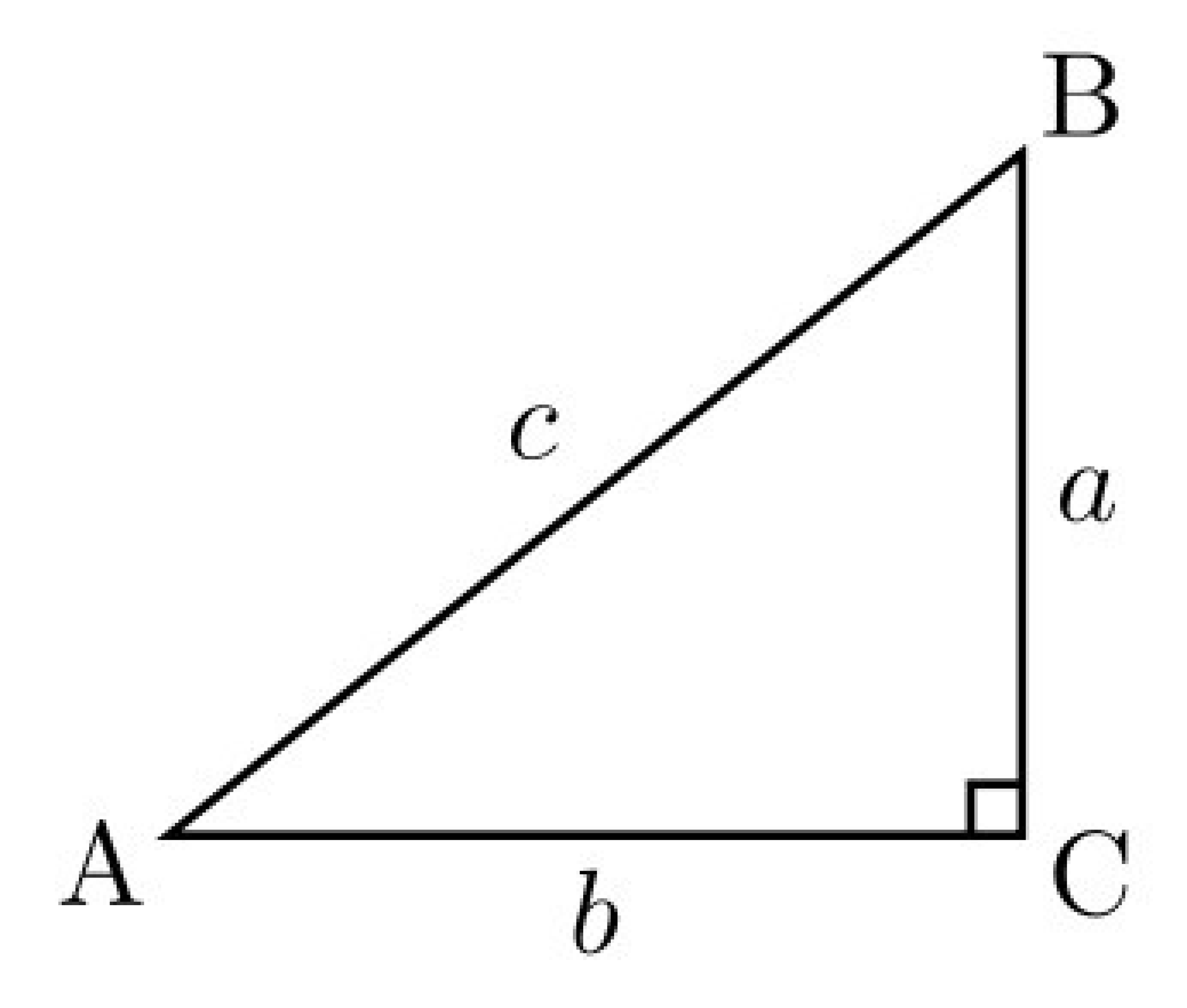
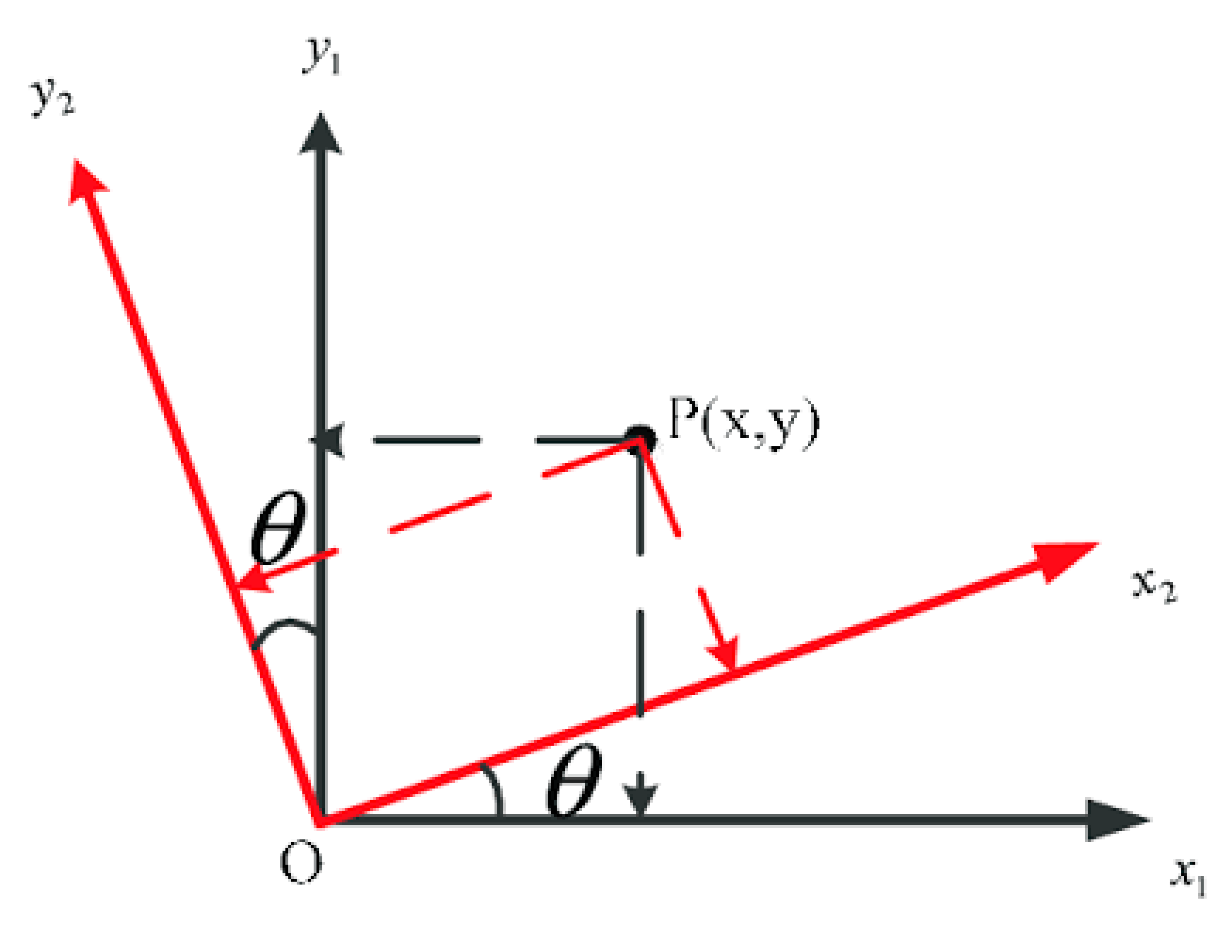
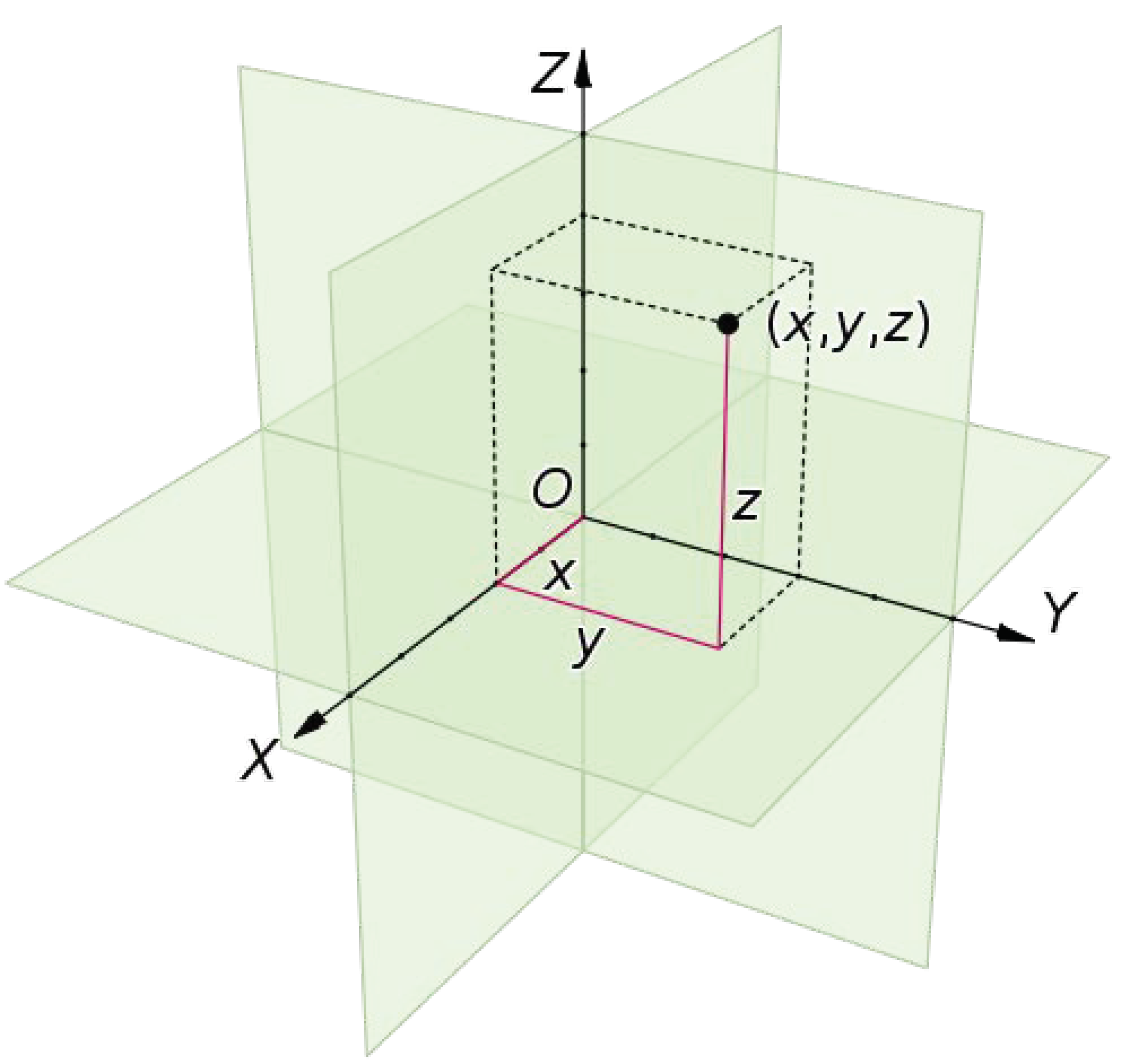
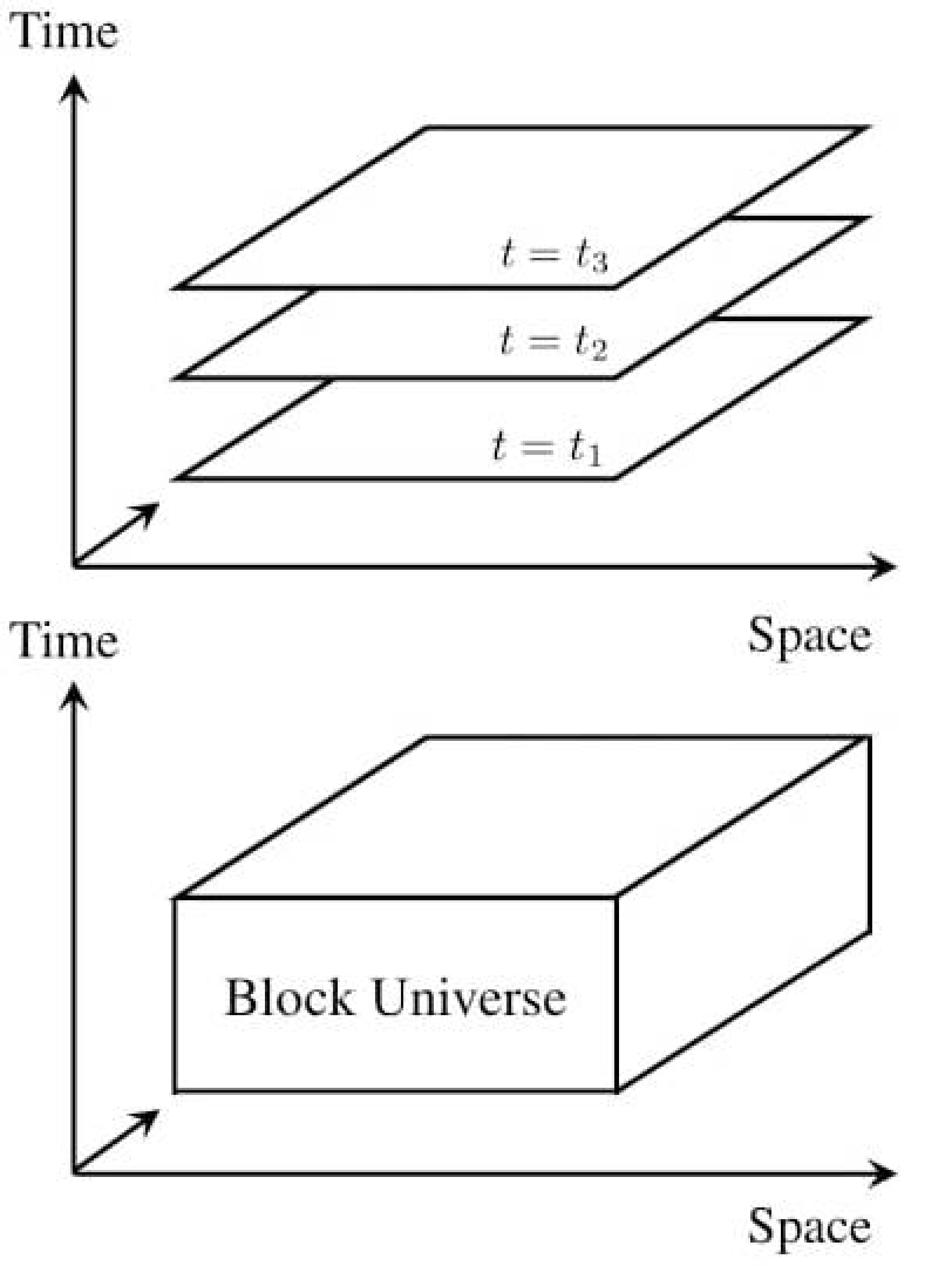
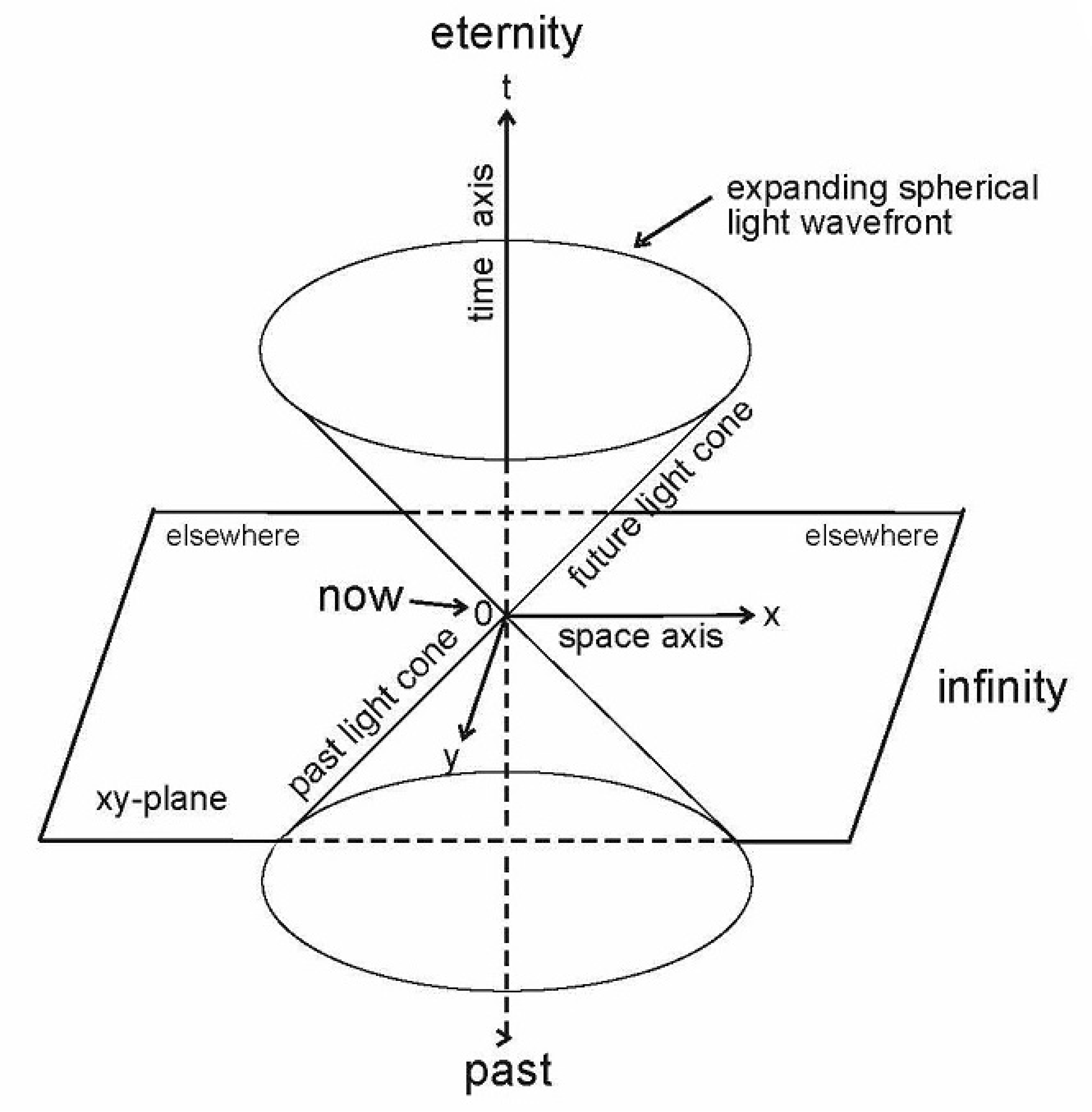
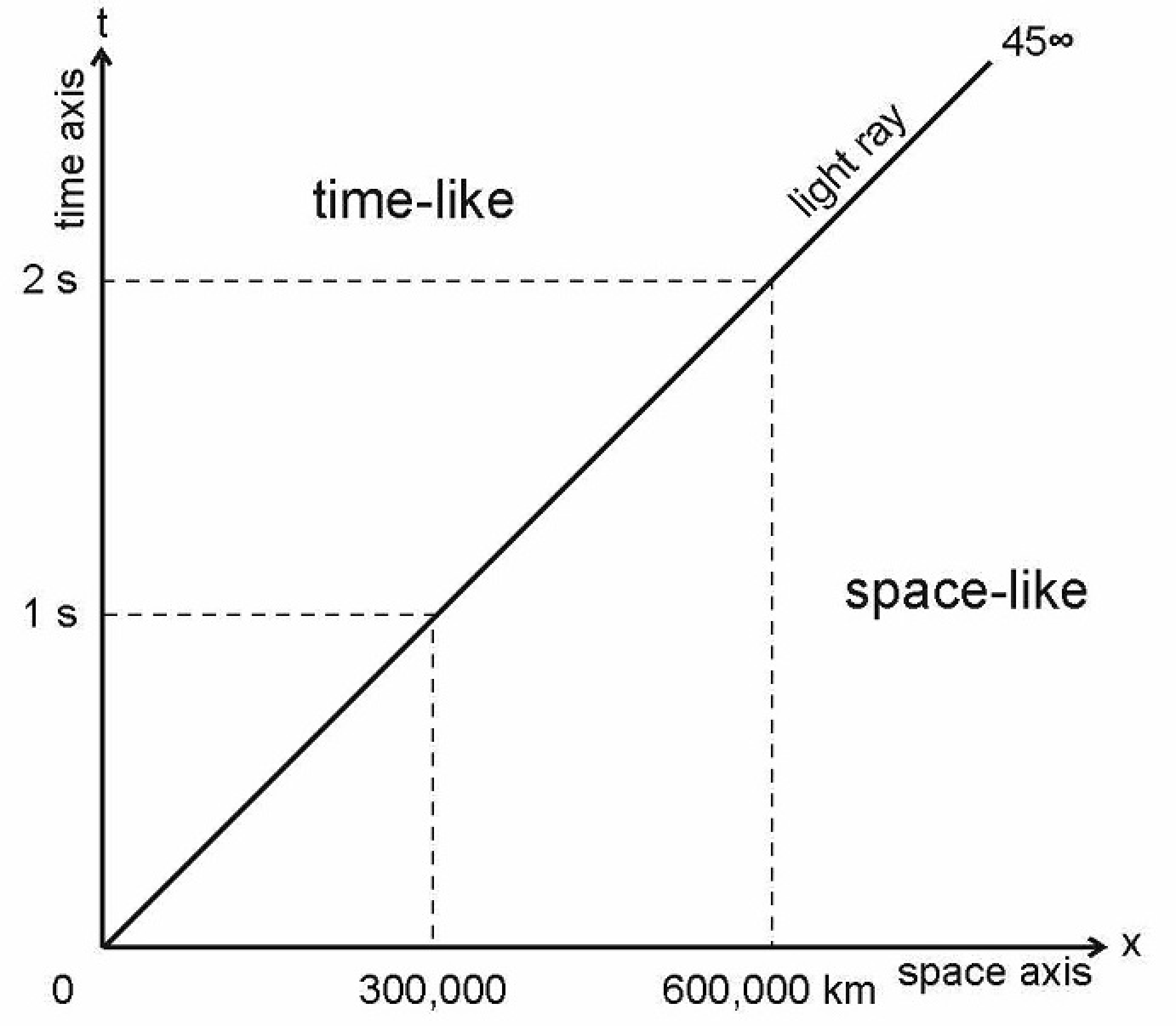
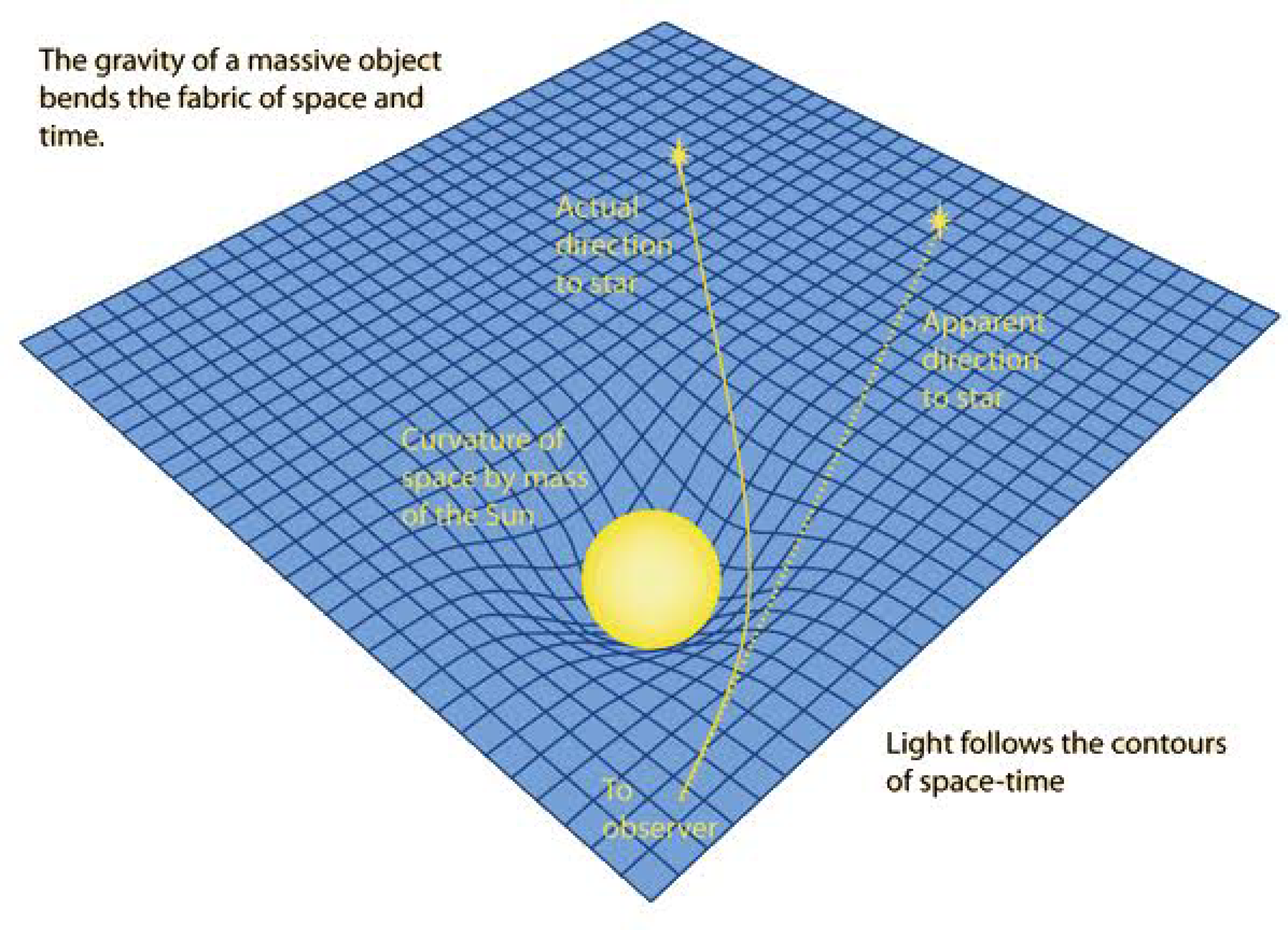
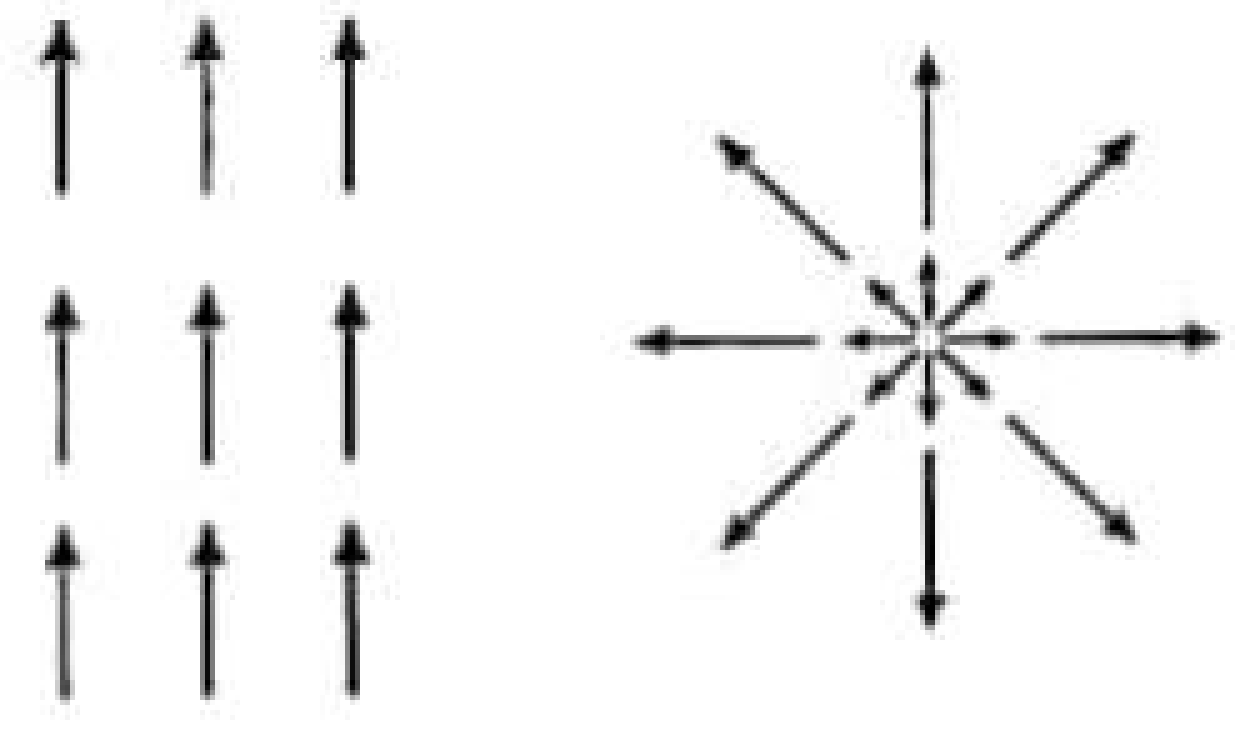
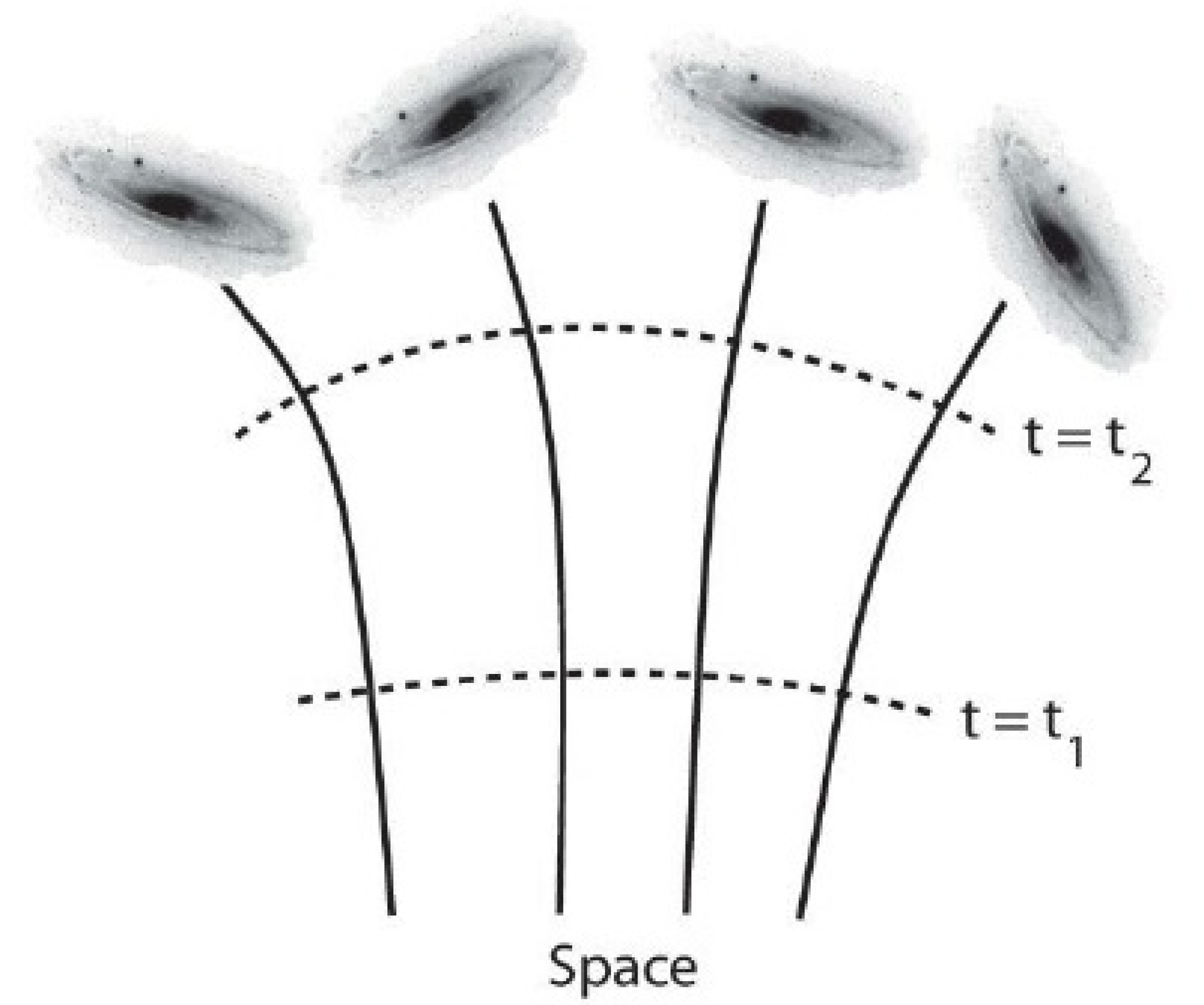
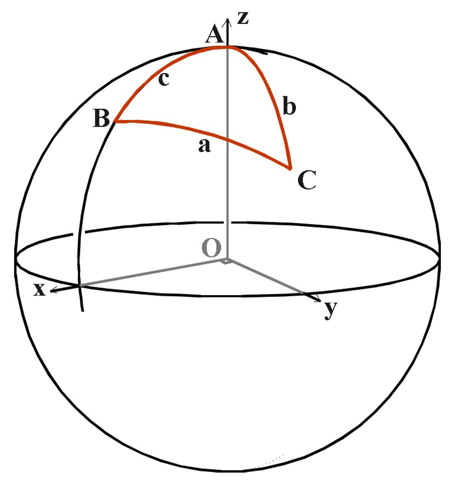
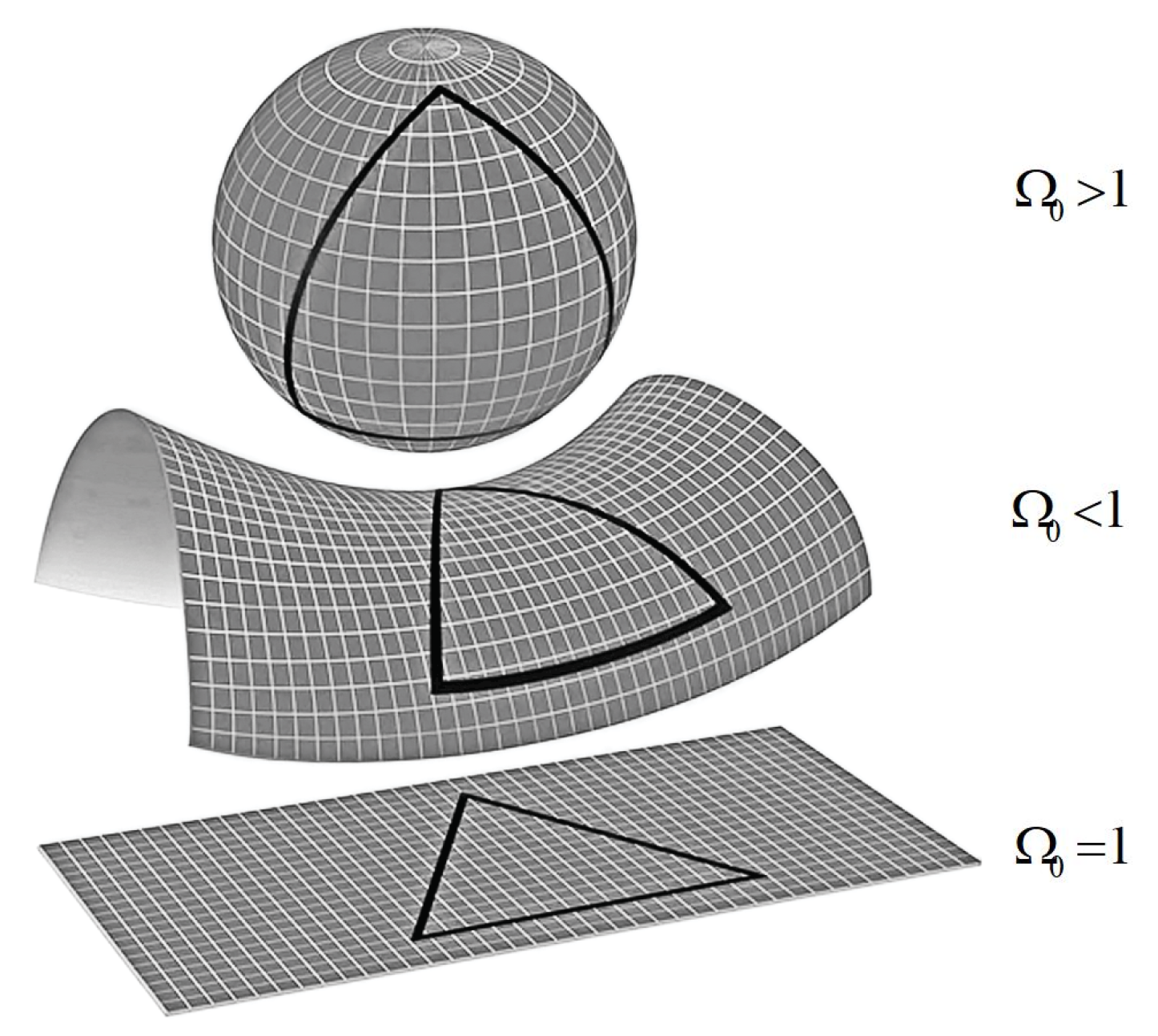
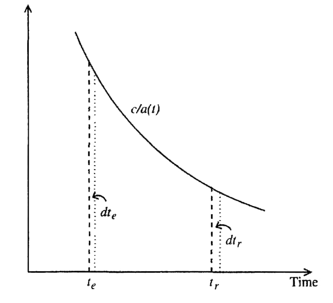
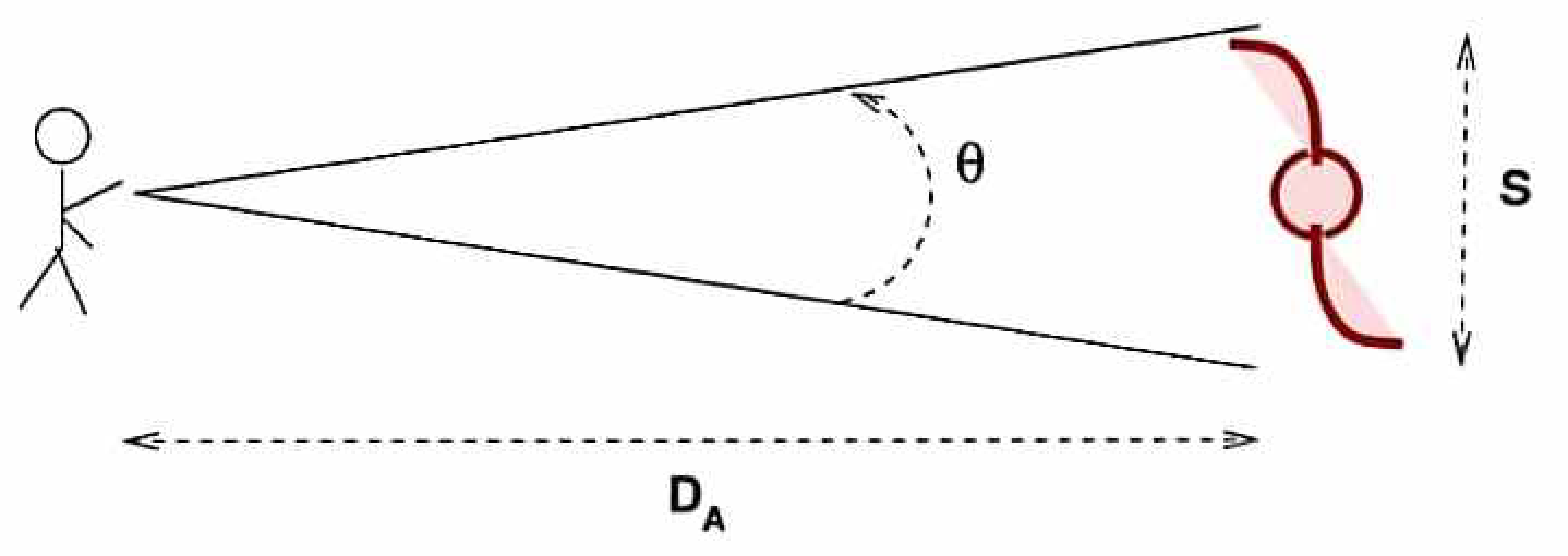
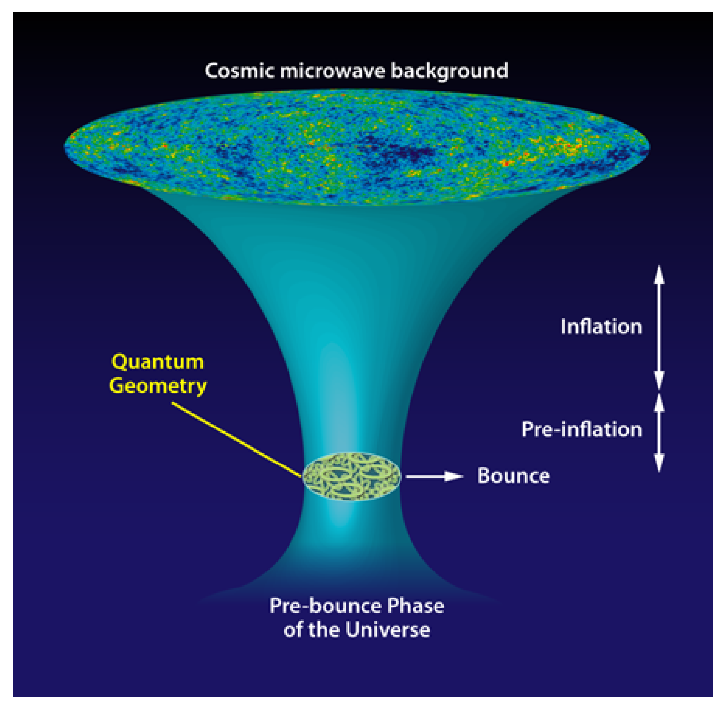
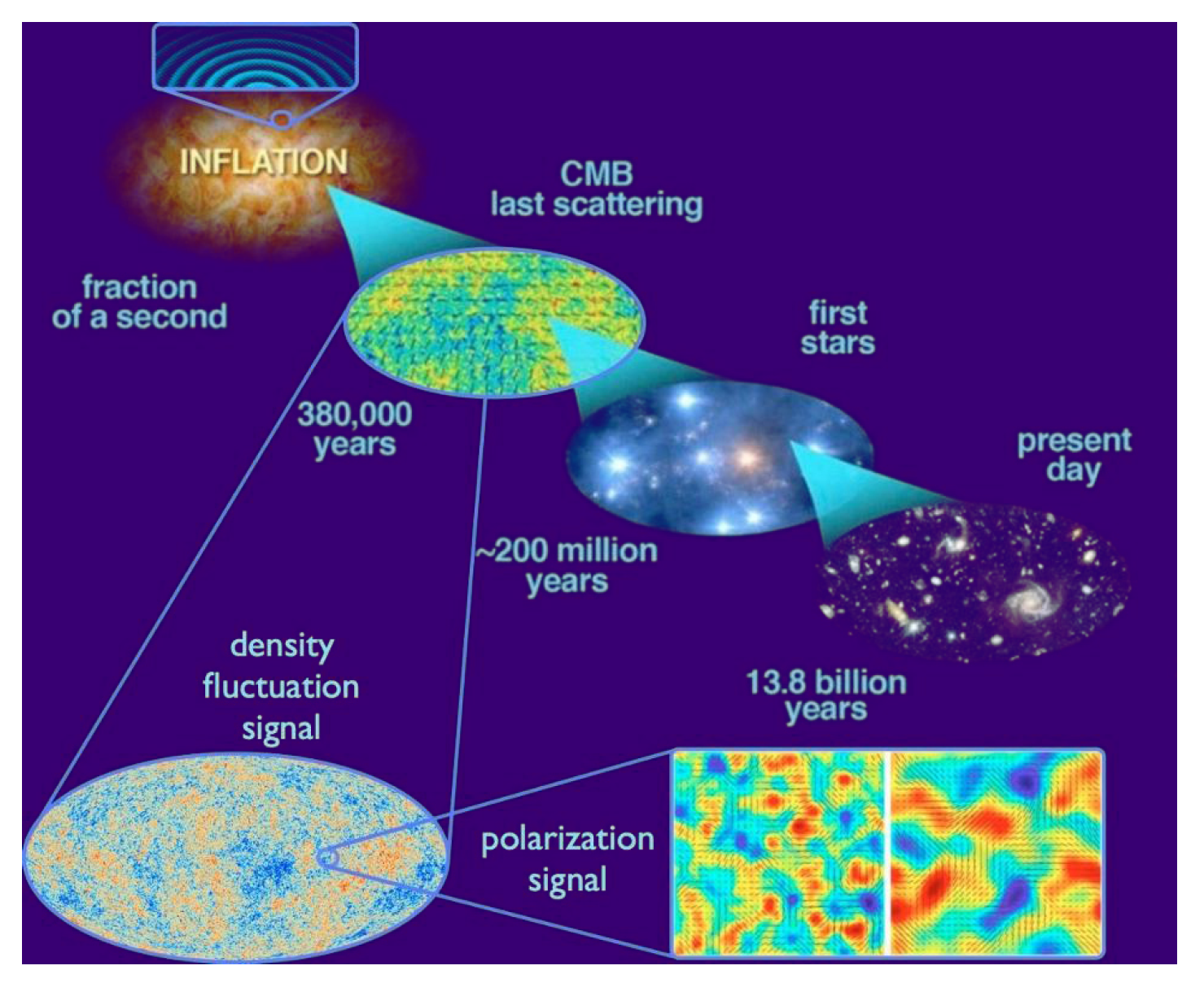
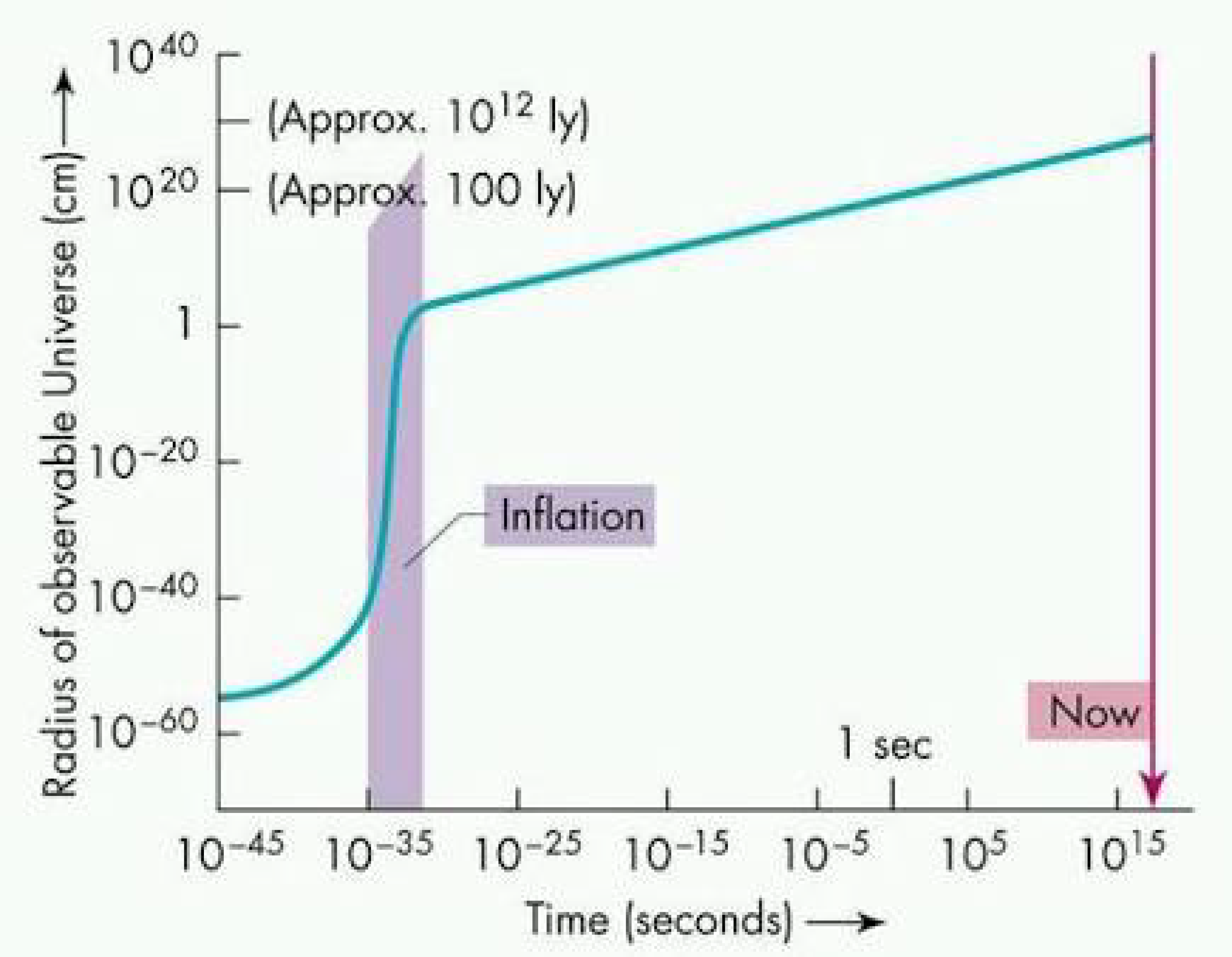
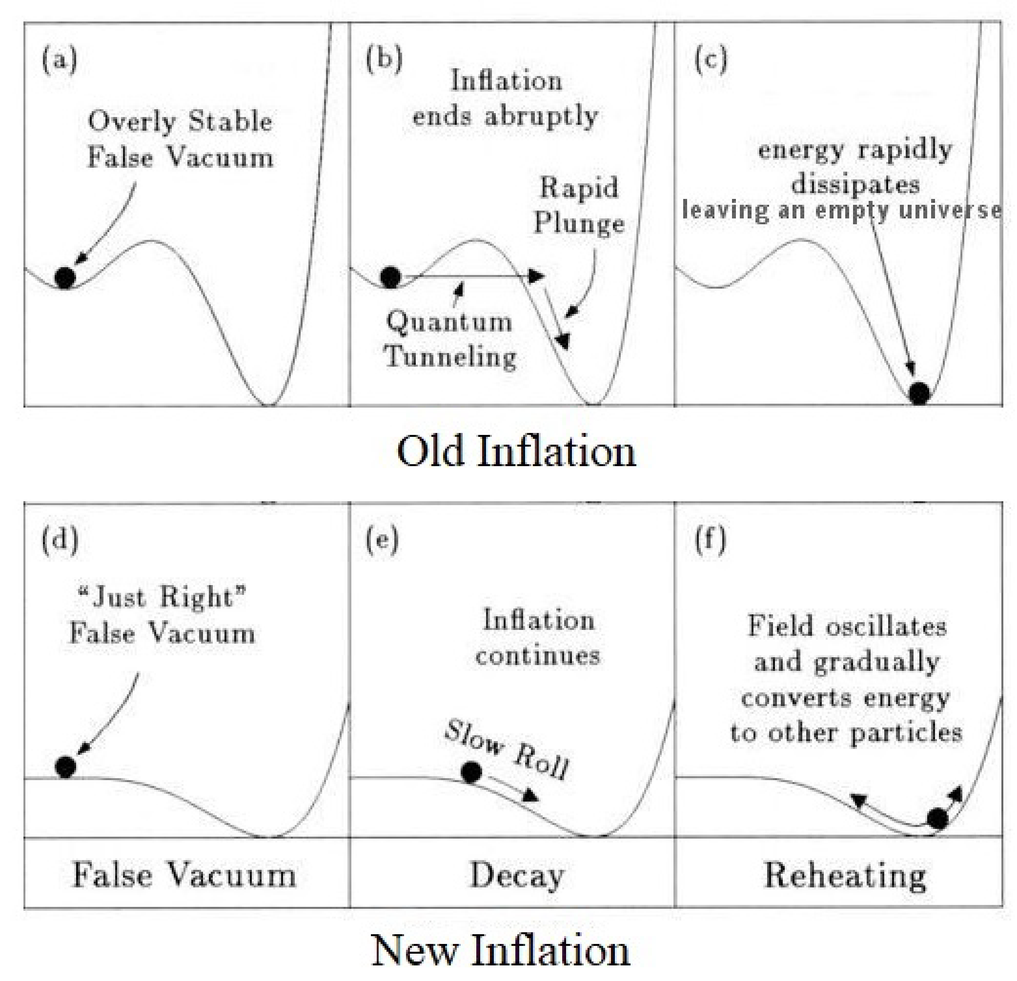
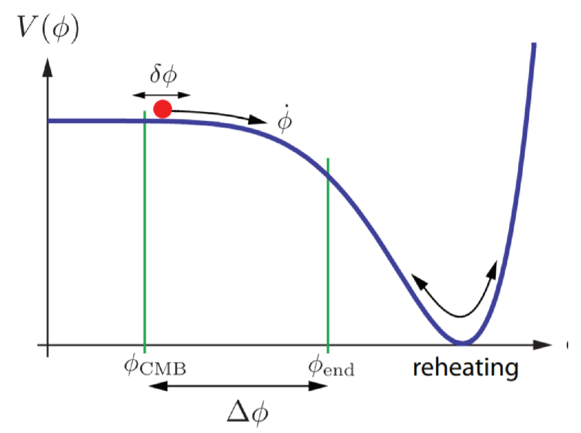
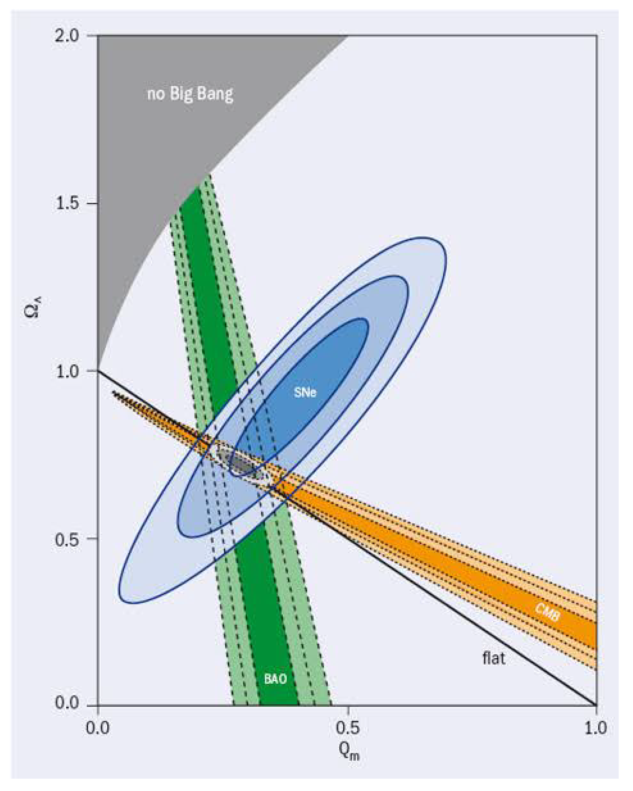
Table 1.
Values of six parameters of CDM from different sources.
| Sr. No | Parameters | CDM | |||
|---|---|---|---|---|---|
| Planck-2018 | Planck-Lowℓ + SPT | Planck-Lowℓ + SPT + BOSS | Planck-Lowℓ + SPT + BOSS + SHOES | ||
| 1 | 0.02233 ± 0.00015 | 0.02269 ± 0.00025 | 0.02250 ± 0.00021 | 0.02255 ± 0.00020 | |
| 2 | 0.1198 ± 0.0012 | 0.1143 ± 0.0020 | 0.1166 ± 0.0012 | 0.1159 ± 0.0010 | |
| 3 | 0.9652 ± 0.0042 | 0.9785 ± 0.0074 | 0.9716 ± 0.0056 | 0.9735 ± 0.0054 | |
| 4 | 3.043 ± 0.014 | 3.021 ± 0.017 | 3.014 ± 0.017 | 3.008 ± 0.017 | |
| 5 | 0.0540 ± 0.0074 | 0.0510 ± 0.0086 | 0.0456 ± 0.0082 | 0.0437 ± 0.0087 | |
| 6 | 1.04089 ± 0.00031 | - | - | - | |
Publisher’s Note: MDPI stays neutral with regard to jurisdictional claims in published maps and institutional affiliations. |
© 2021 by the authors. Licensee MDPI, Basel, Switzerland. This article is an open access article distributed under the terms and conditions of the Creative Commons Attribution (CC BY) license (https://creativecommons.org/licenses/by/4.0/).
Share and Cite
MDPI and ACS Style
Mughal, M.Z.; Ahmad, I.; García Guirao, J.L. Relativistic Cosmology with an Introduction to Inflation. Universe 2021, 7, 276. https://0-doi-org.brum.beds.ac.uk/10.3390/universe7080276
AMA Style
Mughal MZ, Ahmad I, García Guirao JL. Relativistic Cosmology with an Introduction to Inflation. Universe. 2021; 7(8):276. https://0-doi-org.brum.beds.ac.uk/10.3390/universe7080276
Chicago/Turabian StyleMughal, Muhammad Zahid, Iftikhar Ahmad, and Juan Luis García Guirao. 2021. "Relativistic Cosmology with an Introduction to Inflation" Universe 7, no. 8: 276. https://0-doi-org.brum.beds.ac.uk/10.3390/universe7080276
Note that from the first issue of 2016, this journal uses article numbers instead of page numbers. See further details here.