
Lorentzian Vacuum Transitions in Hořava–Lifshitz Gravity


Departamento de Física, Centro de Investigación y de Estudios Avanzados del IPN, P.O. Box 14-740, Ciudad de México 07000, Mexico
*
Author to whom correspondence should be addressed.
Universe 2022, 8(4), 237; https://0-doi-org.brum.beds.ac.uk/10.3390/universe8040237
Submission received: 21 March 2022
/
Revised: 8 April 2022
/
Accepted: 8 April 2022
/
Published: 12 April 2022
(This article belongs to the Special Issue Quantum Gravity Phenomenology)
Abstract
:The vacuum transition probabilities for a Friedmann–Lemaître–Robertson–Walker universe with positive curvature in Hořava–Lifshitz gravity in the presence of a scalar field potential in the Wentzel–Kramers–Brillouin approximation are studied. We use a general procedure to compute such transition probabilities using a Hamiltonian approach to the Wheeler–DeWitt equation presented in a previous work. We consider two situations of scalar fields, one in which the scalar field depends on all the spacetime variables and another in which the scalar field depends only on the time variable. In both cases, analytic expressions for the vacuum transition probabilities are obtained, and the infrared and ultraviolet limits are discussed for comparison with the result obtained by using general relativity. For the case in which the scalar field depends on all spacetime variables, we observe that in the infrared limit it is possible to obtain a similar behavior as in general relativity, however, in the ultraviolet limit the behavior found is completely opposite. Some few comments about possible phenomenological implications of our results are given. One of them is a plausible resolution of the initial singularity. On the other hand, for the case in which the scalar field depends only on the time variable, the behavior coincides with that of general relativity in both limits, although in the intermediate region the probability is slightly altered.
1. Introduction
The quantum theory of the gravitational phenomena, or quantum gravity, is a theory in construction, which is necessary in order to shed light on the quantum effects of gravitational systems. Among the problems that require the uses of quantum gravity is the study of the microscopic origin of thermodynamic properties of black holes and those describing some cosmological phenomena in the very early universe. Another important problem is the study of the vacuum decay and the transition between vacua at early stages of the evolution of the universe. Euclidean methods have been proposed in order to compute this transition probability by using the path integral approach [1,2,3]. One of the salient features of this approach is the prediction of transitions between open universes [3]. Later an alternative procedure to compute these transitions using the Hamiltonian approach was developed [4,5]. This method incorporates the Arnowitt, Deser and Misner (ADM) Hamiltonian formalism of general relativity (GR) [6,7,8]. The vacuum is implemented through a cosmological constant, which is interpreted as the vacuum energy, and the transitions are carried out through a bubble nucleation [9]. In this approach, the transitions between Minkowski and de Sitter spaces are allowed. Very recently, an approach [4,5] was further developed by Cespedes et al. [10] where the vacuum is implemented by the minima of a potential of a scalar field in the curved space. In this reference, it was computed the general vacuum decay transitions in the Hamiltonian formalism in Wheeler’s superspace and some examples were implemented in the minisuperspace formalism for the Friedmann–Lemaître–Robertson–Walker (FLRW) cosmology. In this kind of model, it was shown that the transitions between closed universes are allowed, contrary to the Euclidean approximation of Coleman and De Luccia [3]. Later, the formalism of [10] was extended and used to obtain the vacuum decay transition probabilities for some examples of transitions between anisotropic universes [11].
On the other hand, it is well known that GR is not a renormalizable theory. Thus, its application to very small distances such as those associated with the early universe is expected to fail. Instead of that, an important proposal to describe the quantum effects of gravity is the Hořava–Lifshitz (HL) theory [12] (for some recent reviews, see [13,14,15,16] and references therein). Hořava–Lifshitz theory is a theory with an anisotropic scaling of spacetime and, consequently, it is not Lorentz invariant at high energies (ultraviolet (UV)). However, it is a well-behaved description at small distances due to the incorporation of higher order derivative terms in the spatial components of the curvature to the usual Einstein–Hilbert action, giving rise to a ghost-free theory. Thus, this theory is more appropriate to describe the quantum effects of the gravitational field, such as the vacuum decay processes in the early stages of the universe evolution.
It is important to remark that HL theory is a theory whose low energy limit which connects with GR is troublesome. The parameters of the theory are the critical exponent z and the foliation parameter . This last parameter is associated with a restricted foliation compatible with the Lifshitz scaling. In the low energy limit , the Lorentz invariance is recovered. In the infrared (IR) limit, the limit is accompanied by the limit , where the full diffeomorphisms symmetry is recovered and, consequently, the usual foliation of the ADM formalism is regained. In addition, the higher order derivative terms in the action have to be properly neglected in order to obtain the correct limit. As we mentioned before, the GR limit is problematic since it remains an additional degree of freedom (in some cases interpreted as dark matter) which leads to a perturbative IR instability [14,16,17,18]. The non-projectable version of the HL theory has the possibility to remove this unphysical degree of freedom. Thus, it represents an advantage over the projective theory. However, in the case in which one is concerned with the Wheeler–DeWitt (WDW) equation, both approaches give the same result. In consequence, we will work with the projectable version.
Since HL theory represents an improvement over GR in the high energy regime, it is natural that quantum gravity aspects of the theory are of great interest. Indeed, canonical quantization of the theory has been extensively studied. For example, some of the papers describing solutions for Hořava–Lifshitz’s gravity in quantum cosmology in the minisuperspace are [19,20,21,22,23,24,25].
As we mentioned before, HL gravity is a UV completion of GR, thus, it is a more suitable arena to study the vacuum transitions in the presence of a scalar field potential. This proposal will be carried out in the present article. In order to do that, we use the Hamiltonian formalism of the HL theory, in particular the WDW equation will be discussed in this context following [10,11]. We will particularly focus on the closed FLRW universe and study two types of scalar fields. First, since the anisotropic scaling of spacetime variables is a key ingredient of HL theory, we will consider a scalar field which is allowed to depend on all spacetime coordinates. Lastly, we will also consider a scalar field which only depends on the time variable as it is more usual on the cosmological models.
This work is organized as follows. In Section 2 we give a brief review of the general procedure presented in [11] to study vacuum transition probabilities between two minima of a scalar field potential in the minisuperspace following the formalism of [10]. We will show that this formalism implemented for GR in [10,11] is sufficient to study vacuum transitions in a more general theory, such as HL theory. Section 3 is devoted to obtaining the WDW equation in the context of gravity coupled with matter. In Section 4, we study the vacuum transitions in HL gravity for the scalar field depending on all spacetime variables. The IR and UV limits for the transition probabilities are discussed and compared to the GR result. Then, in Section 5, we study the transition probabilities for the scalar field depending only on the time variable and we also compare the result to the GR one. Finally, in Section 6, we give our conclusions and final remarks.
2. Vacuum Transitions for a Scalar Field
In this section, we review the procedure to obtain a general expression for the transition probability between two minima of the potential of a scalar field by obtaining a semi-classical solution to the WDW equation using a WKB ansatz described in Ref. [11]. We follow closely the notation and conventions given in that reference. It is a remarkable point to see that this procedure is enough to implement theories more general than GR such as the HL gravity.
We start by using the well-known ADM-formulation of GR [6,7,8] and consider the Hamiltonian constraint expressed in the general form:
where we take the coordinates in Wheeler’s superspace to be with (which has in general an infinite number of dimensions). These variables are the components of the three-dimensional metric, the matter field variables, etc. and are denoted collectively as . Their corresponding canonical momenta are and the inverse metric in such space is . Finally, is a function that represents all other additional terms, such as the term and the potential terms of scalar field in the WDW equation. The general WDW equation that we are going to consider is obtained after carrying out the standard canonical quantization procedure of the Hamiltonian constraint. Thus performing this procedure we obtain:
where represents the wave functionial which depends on all fields of the theory.
We are interested in obtaining a semi-classical result, therefore, following [10,11] we consider an ansatz of the following WKB form where S has an expansion in ℏ in the usual form:
Inserting Equation (3) into Equation (2) and focusing only on the term at the lowest order in ℏ we obtain:
On a certain slice of the space of fields a set of integral curves can be specified in the form:
where s is the parameter of these curves. The classical action appearing in the previous equation has the form:
We note that we have a system of equations for the variables: defined by (5) and (7). Thus, we can obtain a solution for such a system and then substitute the results back into Equation (6) to obtain the classical action. Therefore, in principle, we have enough information to compute the classical action, and consequently, the wave functionial to first order in ℏ regardless of the number of fields in superspace.
Under the ansatz that all the fields on the superspace depend only on the time variable, we can obtain a general solution to the system in terms of the volume Vol of the spatial slice X of the form:
In this article, we will consider gravity coupled to a scalar field provided by a potential which has at least a false and a true minima. Moreover, we will study wave functionals such that the scalar field produces a transition between two minima of the potential.
One can use these wave functionals in order to compute the transition probability with the standard interpretation that these transitions are due to a tunneling between the two minima of the potential involved in the transition. In order to be more precise, in the semi-classical approximation, the probability to produce a transition between two vacua at and is the decay rate which can be written as:
where denotes all other fields defined on the superspace except the scalar field, is the wave functional associated to the path which starts in , and where the scalar field takes the value . Moreover, the path ends in , where the scalar field is denoted by . Furthermore, and are the constants of the linear superposition. In the previous equation, we will consider just the dominant contribution of the exponential terms. Then, in the WKB approximation at first order yields:
where the choice of the signs ± indicates the dominant terms in the expression (10). Thus, we finally arrive at the transition probability given by:
It is worth mentioning that the formalism developed in [10,11], originally for GR, is general enough to include other gravitational theories, since it only depends on a Hamiltonian constraint written in the general form (1). In the next sections, we will show that it can perfectly include higher derivative generalizations of GR as the HL theory. It would be interesting to study to what extent this formalism can be used for more general theories.
3. Wheeler–DeWitt Equation for Hořava–Lifshitz Gravity Coupled to Matter
In this section, we will discuss the action in HL theory, as well as the action that considers the coupling to a scalar field. We will consider a metric describing an FLRW universe and a scalar field depending on the time variable, as well as the spatial variables, and we will obtain the WDW equation for such a system. Although in the context of cosmology it is usual to use a time-dependent field only, in this case, we will allow the scalar field to also depend on the spatial variables since the anisotropic scaling of both sets of variables is a key ingredient for the theory. This type of dependence has been used previously in the context of cosmology for HL. For example, it was used in Ref. [26] to study perturbations coming from a scalar field. However, for completeness and correspondence with the cosmological models, we will also study the case when the field will only depend on the time coordinate in Section 5.
Let us begin by considering the gravitational part of the general action in projectable HL gravity without a cosmological constant and without detailed balance. This action can be written as [19,27,28]:
where N is the lapse function, the Ricci tensor with the spatial indices, R the Ricci scalar, the extrinsic curvature, the Planck mass, D denotes covariant derivative with respect to the three-metric and h denotes its determinant, all () are positive dimensionless running coupling constants and the parameter runs under the renormalization group flow. GR is, in principle, obtained in the limit and . However, this is not actually fulfilled because of the perturbative IR instability and the presence of an unphysical degree of freedom as mentioned in the introduction.
Let us take the FLRW metric with positive curvature that describes a closed homogeneous and isotropic universe. This metric is written as:
where, as usual, , and . In the context of the ADM formalism, we note that for this metric:
and therefore, we will work with a projectable version of HL gravity. Substituting these values in the action (13) we obtain that for this metric the gravitational action reads:
where a dot stands for the derivative with respect to the time variable. The integral for the spatial slice has been performed, that is:
In order to couple a scalar field (where denotes collectively the three spatial variables) to this theory we need to consider actions that are compatible with the anisotropic scaling symmetries of the theory and UV renormalizability. In fact, the general scalar action in HL gravity is found to contain up to six order derivatives. This action is written in the form [29]:
where the function is given by:
with denoting the three-metric laplacian and is the potential for the scalar field. The constant is the velocity of light in the IR limit, whereas the two other constants are related to the energy scale M as:
There are three more possible terms that can be part of (19) constructed as products of derivatives, but we restrict ourselves to the terms just described.
Since the three-metric derived from the FLRW metric is just a scale factor times the metric of the three-sphere , we can use the spherical harmonic functions defined in this space to expand our scalar functions [30,31]. These functions can be defined in our spatial three-metric as eigenfunctions of the laplacian of the form:
where n is an integer. They obey the orthonormality condition:
Since these functions form a complete basis, we can expand any scalar function defined on the sphere in terms of them as:
Therefore, using this basis, we can expand the scalar field as:
where the fields are real functions depending only on the time variable. We can also expand the scalar field potential as:
where the function depends on all the functions in general. Substituting (24) and (25) back into the action (18), we observe that for the FLRW metric the field part of the action is written as:
where and
are constants. Finally, by considering both actions (16) and (26), we observe that the full lagrangian describing HL gravity coupled to a scalar field is:
We observe, in this case, that the degrees of freedom are the fields . Their canonical momenta turn out to be:
and, as it is usual, the lapse function is non-dynamical since . Therefore, we obtain that the Hamiltonian constraint takes the form:
4. Vacuum Transitions in Hořava–Lifshitz Gravity
Now that we have obtained the Hamiltonian constraint of the HL gravity coupled to a scalar field depending on all spacetime variables, let us study the probability transition between two vacua of the scalar field potential. We note that the form of the Hamiltonian constraint (30) as obtained in the previous section is of the same general form as the one considered in (1) taking the coordinates on superspace to be . The inverse metric is given by:
where denotes a vector with length equal to all the possible values that the set can have and with 1 in all its entries. In this case then we also have:
Therefore, the general procedure to obtain a solution of the WDW equation presented in Section 2 is applicable to the WDW equation obtained after quantizing the Hamiltonian constraint (30) in HL gravity. In order to study transitions between two vacua of a scalar field potential, we consider that all fields appearing in the expansion of the potential (25) have the same minima, namely, one false minimum at and one true minimum at , and therefore, the two minima of the scalar field comes only from its time dependence. Therefore, the transition probability in the semi-classical approach between these two minima is given by Equation (12).
Following [11], we can choose the parameter s such that for the interval , where is the initial value, the field remains close to its value at the true minimum , and for the interval the field remains very close to its value at the false minimum , that is, we choose the parameter s such that:
However, in this case, taking the expansion (24) and since the spherical harmonics are an orthonormal set, the latter implies that:
and similarly for the potentials
Consequently, the logarithm of the probability (11) is given in this case by:
We note that this term has the same form as the one considered in Refs. [10,11] regarding the portion of the integral in which the scalar field can vary, therefore, we can also interpret this term as a tension term taking:
Although this function has no minima in the points considered, it is a function of the scalar fields that can be interpreted as a new effective potential with the form of a mass term. Therefore, applying the same logic used in [11] to such terms, we can define a new contribution for the tension term as:
Similarly, we define for the two remaining terms:
and the two contributions to the tension terms as:
On the other hand, in order to do the two first integrals in (38) where all scalar fields are constants, we use the general solutions (8) and (9), then, after changing the integration variables from s to a according to we obtain:
where
Therefore, substituting Equations (41), (44), (46), (47) and (48) back into (38) we obtain:
where we have defined the function:
and it is worth noting that in the above result, the sign ambiguity on the left-hand side comes from the arguments leading to Equation (11), whereas the one on the right comes from the fact that the general solution (8) and (9) for the system of equations gives a solution for , which produces a sign ambiguity in Equation (48). Therefore, both ambiguities are independent to each other.
As it is well known, the IR limit of HL gravity for an FLRW metric is achieved in the limit and , and corresponds to GR with an extra degree of freedom albeit with the instability problems mentioned in the introduction section. We note that the kinetic term for the scale factor in (28) is:
In the GR case considered in [11], it is given by:
because the term in that case is a global multiplicative factor to the full lagrangian, it can therefore be ignored. Thus, in order to obtain the same kinetic term in both cases in the limit , we consider units such as . This choice of units will allow us to directly compare the transition probability to the one obtained in GR.
Then, we finally obtain for the logarithm of the transition probability:
with
We note that in contrast to the results obtained using GR for all the types of metrics considered in [11], this transition probability is described by five parameters, and by extremizing the latter with respect to we can at most reduce them by one. It is also important to note that the above integrals cannot be performed explicitly for any values of the constants. Nonetheless, it is an expression valid for any value of the potentials and, interestingly, it is a general expression that does not depend on having to consider the different modes contributing to the expansion in Equation (24) separately.
As it is explained in [10,11], the choice of s as in (33) is useful to obtain exact solutions for the transition probabilities that lead to the same solutions as the ones obtained using euclidean methods. However, there is also room to consider s in different ways. For example, we can also choose s as the distance in field space. This choice allows us to show that we can have classical transitions just because the metric in superspace for the WDW equation considered here coming from the Hamiltonian constraint (30) is non-positive definite, as is the case for all the metrics considered in [11].
Now that we have computed the transition probability for HL gravity in general, let us consider its two limits of importance, namely, the infrared and the ultraviolet limit. The first enables us to directly compare with the result found by using GR and the latter allows us to highlight the contributions for high energies that marks the importance of HL gravity.
Taking the IR limit of (54), that is, taking and , we obtain:
Therefore, we find in the infrared an expression quite similar to the GR result plus one degree of freedom extra coming from the term in the action for the scalar field (26) as expected. In order to directly compare our result to the result obtain for GR, we can, for the moment, set , then the last result simplifies to:
that is the same result obtained for GR in [10,11]. The only difference comes in the choice of , since for the consistency of the integral approximation we have here that , therefore, it cannot be chosen to be zero. Thus, the difference between this result and the GR one are only constants. We also note that the potential appearing in this expression is not the potential found originally in the scalar field action, rather it is an effective potential appearing after integration of the harmonic functions. Considering the thin wall limit and extremizing the above result with respect to we obtain:
Then substituting it back into Equation (57) and choosing the plus sign in the right-hand side we obtain:
Therefore, in this limit, the transition probability is finally described in terms of just one parameter (considering as a constant).
If we take in (57), consider the thin wall limit and rename and , we obtain the result found in [10,11] for GR:
then, extremizing we obtain:
Thus, finally the logarithm of the transition probability in GR is written in terms of just one parameter as:1
We can see from (61) that since choosing the plus sign on the right-hand side of (60) implies that always. The same is true regarding . As we know from [10,11], this choice of sign allows us to obtain the results found using the euclidean approach in [32]. It can be proven that the right-hand side of (62) is always positive and, therefore, in order to have a well-defined probability defined by (12) we choose the plus sign in the left-hand side as well. We note, however, from (58) and (61) that in order to have a well-defined tension we need the terms inside the square roots to be positive. If both potential minima are negative, we see that this is indeed satisfied for all values of . However, if at least one of the potential minima is positive, we see that the tension will only be well defined until is big enough, that is, in this case, the tension term is well defined and consequently the expressions (59) and (62) are valid only in an interval from 0 until an upper bound for .
Let us study now the ultraviolet limit, this is found when . In this limit Equation (54) simplifies to:
We note, however, that since all are positive, and the function defined in (45) is also positive for both minima, the first term is purely imaginary. Therefore, it does not contribute to the transition probability at all and it can be ignored. Thus, we finally obtain in this limit:
However, this expression does not have an extremal with respect to . Then, in this case, the probability is described by three independent parameters. For consistency with the GR result, we will choose the plus sign in the left-hand side of the latter equation, therefore, we note that in order to have a well-defined probability we need the overall sign of the right-hand side to be positive. Thus, we can choose both and to take always positive values.
We can see from the GR result (60), or after extremizing (62), that in any case when . However, for the UV limit of HL presented in (64) we have in the contrary when and then the probability increases as increases. Therefore, in this case the UV behavior is completely different for both theories.
Now that we have studied the two limits of interest. We proceed to compare the full result for the transition probability valid for all (54) to the GR result. As we have said, for consistency with GR we are going to choose the plus sign in the left-hand side and the minus sign in the right, and use the thin wall limit, therefore, we will consider:
If we want to vary (65), we will obtain an expression involving the tension terms and the functions . However, since those functions are defined in terms of square roots, we need the terms inside to be non-negative in order to have well defined tension terms, that is we need that:
We note that in the best scenario, the latter expression implies only a lower bound on coming from the term. In the other cases, it could happen that we obtain a lower and an upper bound for , that is the tension terms would only be well defined over a specific interval, or it could even happen that the latter expression is not satisfied at all for any value of and in that case (65) would not have an extremal. In any case, we see that the extremizing procedure is very dependent on the many parameters of the theory and does not allow us to obtain well-defined tension terms in general, in particular, we never have access to the UV region. Therefore, in order to avoid these difficulties, we are going to compare the results obtained before the extremizing procedure takes place, that is, we will use for the comparison the GR result (60) choosing the signs already mentioned and the HL result (65). Since the HL expression depends on many independent parameters and the integrals cannot be made for any values of the constants involved, we are going to evaluate numerically this expression. Since in the IR limit we saw that after extremizing and T are always positive, we are going to take positive values for these parameters. On the other hand, in the UV limit we saw that we can take and also to be positive. Finally, in order to obtain a well defined probability, we are also going to choose positive values for the remaining free parameter . Thus, we will take positive values for all the tension terms.
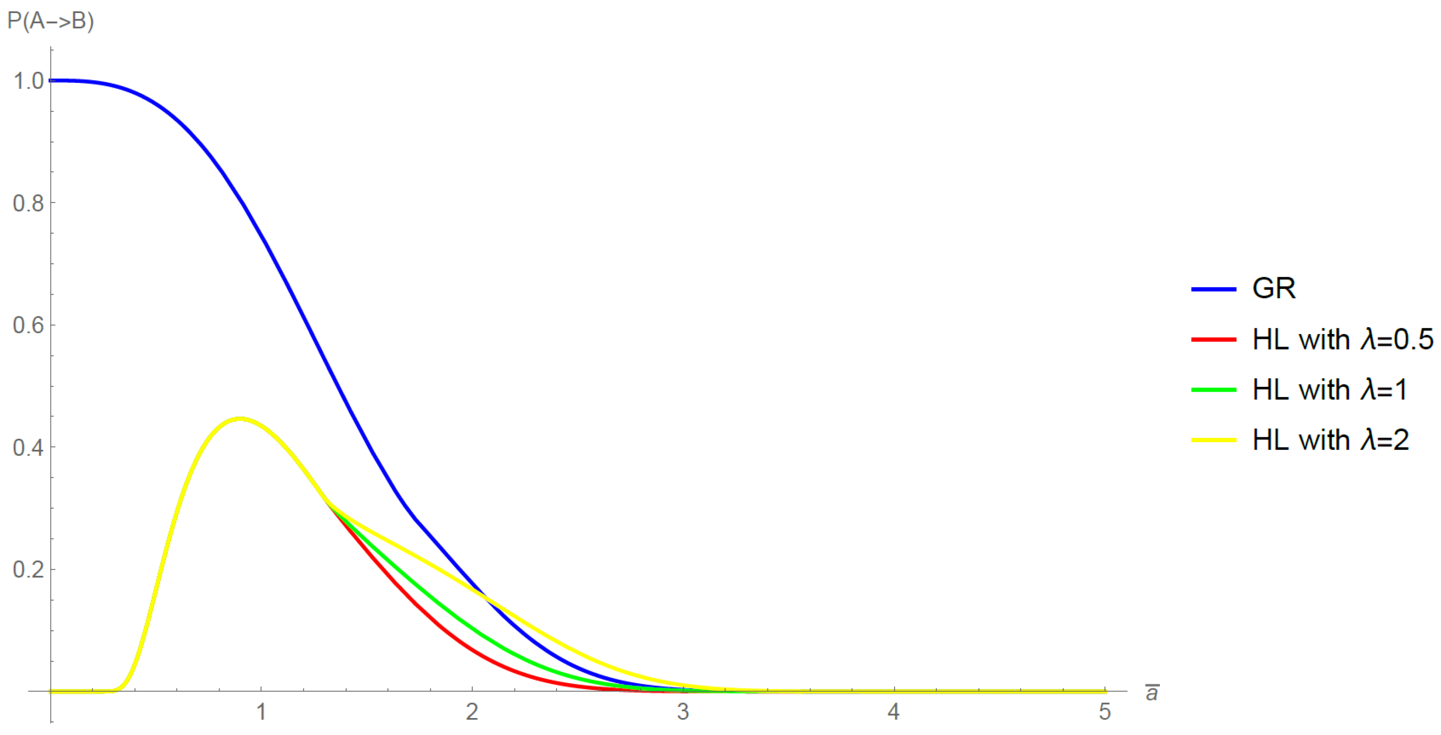
In Figure 1, we show a plot of the transition probabilities coming from the two theories. We choose units such as . For the GR result (blue line), we choose , and . We note that in this case, the first term in (60) is negative, therefore, we need to choose a value for T great enough to obtain a well-defined probability. We see the behavior outlined earlier, that is, the probability goes to 1 in the limit and then it decreases as increases going to zero. For the HL plots, we choose , , , , and , we plot the probability for three different values of to see how this parameter affects the behavior. In this case, we choose in order to compute the integral numerically, however, we know from the UV analysis, that can be chosen without any problem and the general form will be unaltered. In this case, we also have that the first term in (65) is negative and increases with , therefore, we also need to make sure that the tensions chosen are big enough to have a well-defined probability. This figure shows the behavior that we described earlier by studying the different limits of interest. That is, in the IR region, the probability falls in the same manner as the GR result. We note that has to be big enough so the first term can be positive and then contribute to the probability, therefore, the different values of only affect the curve in the IR region and as increases, the probability increases since this term has the opposite sign than the tension terms. In the UV region, the parameter has no impact at all, and then, everything is defined by the tension terms. As we have said earlier, the probability goes to 0 as and then it increases with . We note that this behavior comes from the and terms, that is, it comes from the extra terms in the action for the scalar field (18) and it can be interpreted as the fact that HL avoids the singularity and predicts these types of transitions to occur in a UV regime (small ) but not too close to the singularity. Then, the probability starts to decrease and then it goes into the IR behavior just described. We note that the general form of the plot will be maintained regardless of the values of the parameters, we only have to make sure that they are chosen in a way that the tension terms dominate so we can have a well-defined probability. However, specific things such as the maximum height or the point in which both plots match is completely determined by the parameters and, therefore, we cannot say something about them in general.
In the present section, we have obtained a general formula (65) for the transition probability when the scalar field depends on all spacetime variables. The integrals involved cannot be performed in an analytic form, however, a numerical computation was performed and we showed a plot comparing the results with the one coming from GR. As we pointed out earlier, the UV behavior is found to be completely opposite. This result depends on the extra terms in the action for the scalar fields, however, these terms are only present if we take a field that depends on the spatial variables. Therefore, in the next section we are going to study a scalar field depending only on the time variable.
Phenomenological Remarks
Before we end this section, let us discuss some phenomenological aspects regarding our results. The theory of Hořava–Lifshitz has received a lot of attention and much work has been performed since its first proposal from the theoretical, as well as the phenomenological, point of view. For example, in [33,34,35] the viability of the different versions of the theory have been tested against various experimental (or observational) data sets coming from different sources such as CMB and BAO collaborations. It is found that the theory is in good agreement with such data, and therefore, it supports the importance of considering it as a viable theory. It is also interesting to point out that in these works they always work with an FLRW metric with a non-zero curvature since the flat metric gives the same predictions as in General Relativity. Thus, the importance of studying such metrics as the one we studied in the present article is also supported by these works.
On the other hand, in the vacuum decay process studied by using the euclidean method, discussed in [3], the process is described by the nucleation of true vacuum bubbles and its corresponding expansion. This could lead to phenomenological predictions regarding this kind of phase transitions occurring at some point in the evolution of the universe. However, as it was pointed out in [10] the process studied by using a Hamiltonian approach in the minisuperspace is limited. In fact, in the transition studied, there is no notion of bubble nucleation, we can only compare two configurations of three-metrics and then interpret its ratio as a transition probability. Therefore, it is speculated that this formalism is not describing the same process as the euclidean method. It is believed that it may describe a generalization of the tunneling from nothing scenario, that is, we are obtaining probability distributions of creating universes from a tunneling event between two minima of the scalar potential. If we take seriously this interpretation, then the scale factor appearing in the expression found for the transition probability would correspond to the value that the scale factor of the created universe would have at the time of creation (its corresponding ‘size’). Then, the plot in Figure 1 would tell us that in Hořava–Lifshitz gravity, in the case in which the scalar field depends on the spatial variables, the universe would be created with a scalar factor different from zero, and therefore, we would avoid the singularity contrary to GR which predicts a singularity at the beginning of the universe. This, of course, would have potential phenomenological consequences in the physics of the early universe and its corresponding evolution. Therefore, although we are in a speculating phase, these kinds of transitions are worth studying in more detail.
5. Transitions for a Time-Dependent Scalar Field
In the previous sections, we studied a scalar field depending on all coordinates of spacetime and found a transition probability whose behavior differs completely in the UV regime comparing to the GR result. However, in cosmology it is more common to study a scalar field depending only on the time variable as is the case in [29,36,37]. Therefore, in this section we will consider such a dependence for the scalar field and study the vacuum transition probability between two minima of the potential.
In this case, the scalar field action (18) reduces to:
where we have redefined the scalar field potential appearing in (19) as so it coincides with the usual scalar potential in the action. Since now we have a global factor of as in the action of the gravitational part (16), we can omit this factor. Then, the lagrangian this time is given by:
Therefore, we have only two degrees of freedom a and , their canonical momenta are:
and the Hamiltonian constraint takes the form:
Comparing this last expression to the general form considered in Equation (1), we note that in this case the coordinates in superspace are with inverse metric:
and we also have
In order to study transitions between two minima of the potential, we choose the parameter s as in expression (33), then, following a similar procedure as in the previous section, we obtain in this case that choosing units such as (as in the GR case) and in the thin wall limit, the logarithm of the transition probability is written as:
where
the function F is defined in (51) and as we have mentioned in Section 4, the sign ambiguities in the last expression are independent.
Now that we have computed the transition probability in general, we move on to study its behavior in the limiting cases considered before. For the IR behavior, we consider and in the above expression, the result is the same as in (57) with the same subtlety about as discussed in the previous section. On the other hand, in the UV limit we have . However, in this limit we obtain as . Therefore, we note that the general behavior of these results is the same as the GR result in both extreme cases. In fact, we can variate (73) with respect to to obtain:
Substituting it back in (73) we obtain finally:
Thus, the transition probability is also written in terms of just one parameter as in the GR result. Therefore, the only difference between GR and HL in this case is that the transition probability changes by acquiring two more terms in the square root before integration, making the integral not possible to be performed in general and a global factor depending on in (76). The qualitative behavior in both the IR and UV limit is unaltered.
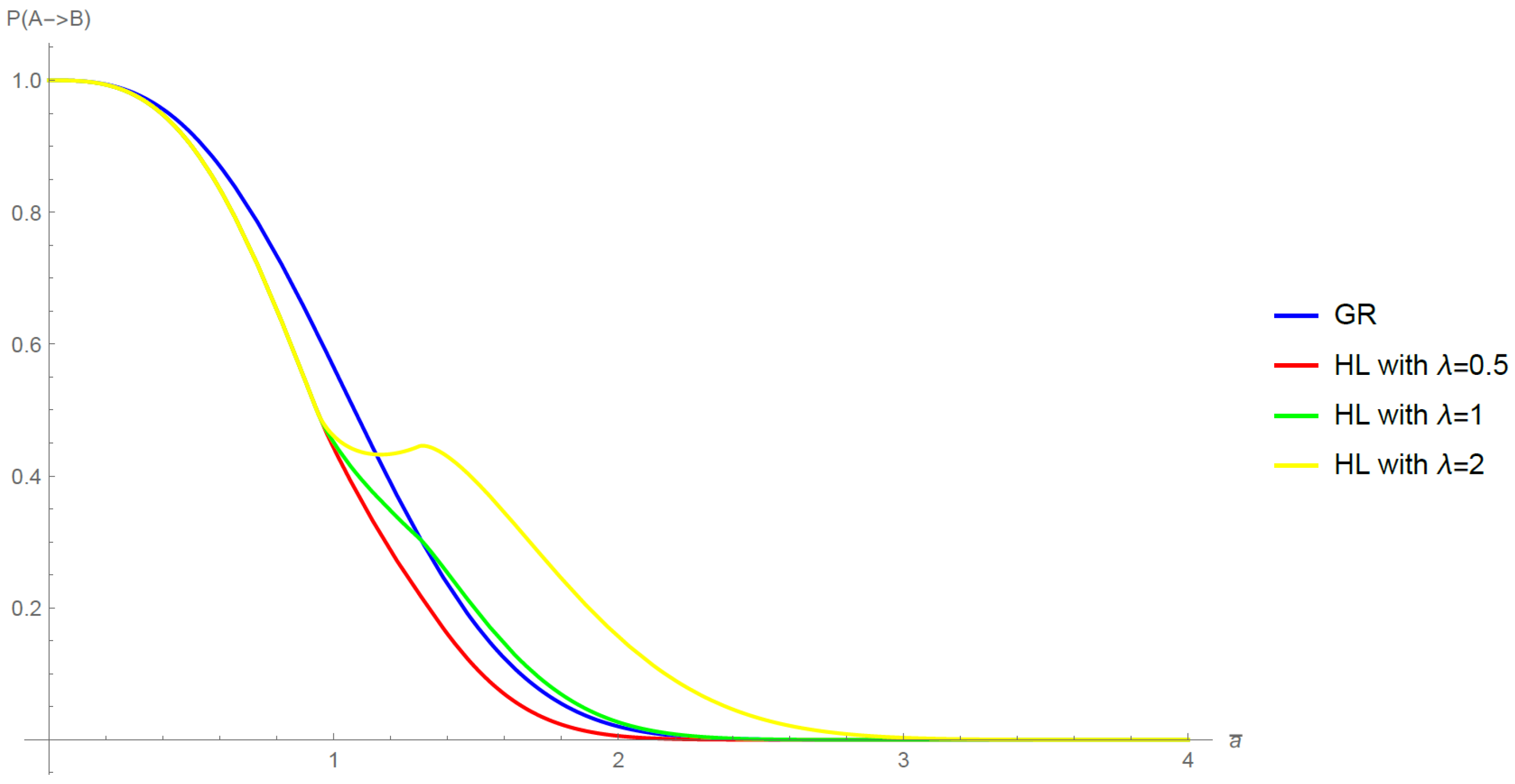
In order to compare the result of this section with that of GR in general, not only on the limiting cases, we note that as in the last section, the extremizing procedure leading to Equation (75) gives rise to some restrictions for the validity of (76). In particular, it is never well defined when is small. Therefore, we are going to use the result (73) and choose the minus sign in the right-hand side so in the IR limit it coincides with the GR result and on the left-hand side we will choose the plus sign in accordance with the GR result as well. We will compare it with the GR result (60) with the sign choices made in the above section. In both cases, we will take the tension T as an independent positive parameter and take values big enough so we can have a well-defined probability and compute the integrals numerically. In Figure 2, we show such a comparison. We choose units such as , with , , and . For the HL result we show plots for three values of and choose in order to perform a numerical computation of the integrals, however, doing the UV limit we note that is possible and it has the same behavior. This figure shows the limiting behavior that we described earlier, that is, in the IR and in the UV limits all curves behave in the same way, it is in the middle region where their behavior is modified. In particular, we note that in the beginning the HL probability is smaller than the one of GR, and the contribution of the parameter is not noticeable; however, when the first term in (73) is big enough, the contribution of the first term is big enough to separate the curves, and as in the case considered in the previous section, as increases the probability increases. Finally, the three probabilities fall as in the GR case.
6. Final Remarks
In the present article, we have studied the transition probabilities for an FLRW metric in Hořava–Lifhitz gravity using a WKB approximation to the WDW equation. The general procedure proposed in [10,11] was found to be applicable to this case. We used HL theory without detailed balance and consider an FLRW metric with positive spatial curvature.
We considered two types of scalar fields. First, since the anisotropic scaling between space and time variables is a key ingredient of HL theory, we considered a scalar field which depends on all spacetime variables. This type of dependence is useful to study cosmological perturbations coming from scalar fields [26]. On the other hand, since in cosmology it is customary to propose an ansatz in which the scalar field depends only on the time variable, we studied this kind of dependence as well. For both cases, we found analytic expressions for the logarithm of the transition probabilities in the thin wall limit.
For the scalar field, depending on all spacetime variables, the transition probability (65) was found to depend on five different parameters coming from the new terms present in the action for gravity, as well as the action from the scalar field in HL theory. There is only the possibility to reduce just one of these parameters after an extremizing procedure but such a procedure is not well defined for all values of the scale factor. Taking the IR limit we found that one degree of freedom extra coming from the scalar field action survives, which is a common issue regarding the IR limit of HL theory. However, if we ignore this contribution, we can obtain an expression that differs from the GR result just by constants. In the opposite limit, that is, in the UV limit, we found that the probability is described in terms of three independent parameters and it vanishes in the limit . This is opposite to the GR result in which the probability goes to 1 in that limit. We interpret this result as a way in which HL theory avoids the spatial singularity at and predicts these transitions to occur on the UV regime but away from the singularity. We note that this behavior comes from the terms in the scalar field action with spatial derivatives, and therefore, it is only possible in the case in which the scalar field depends on the spatial variables. In order to visualize these behaviors, we plotted the transition probabilities coming from GR and HL theory. Such plots were presented in Figure 1. For the HL results, the integrals involved were performed numerically and we saw that in all cases the probability begins at zero with , then it increases with until at some point it starts to decrease and then it behaves as in the GR case. We noted that the first behavior in the UV region is independent of the parameter and it is only on the IR where the dependence on this parameter is noticeable making the probability increase as increases.
For the scalar field depending only on the time variable, the logarithm of the transition probability found have the same number of independent parameters as the GR result, that is, after extremizing we only have one parameter left. However, it also has dependence on the many constants appearing in the extra terms in the gravity action for HL theory, as well as in the parameter . The behavior of the probability in this case is found to be the same as the GR result in both the IR, as well as the UV limits. In fact, in the IR limit, we obtain the same expression as the one coming from the scalar field with dependence in all spacetime variables when we ignore the degree of freedom that survives this limit and in the UV regime we also found that the probability goes to 1 in the limit . Therefore, with a cosmological ansatz, the behavior in the UV regime found by using GR is unaltered. However, in the intermediate region, the probability is of course modified. In order to visualize the difference in this region, we plotted the transition probabilities coming from GR and HL theory and showed them in Figure 2. In this case, we also carried out a numerical computation of the integrals involved in the HL result. We noted that, at first, the probability of HL is smaller than GR and the contribution from the parameter is not noticeable. However, when the scale factor is big enough, this contribution is important and, as in the latter case, the probability increases with . It is interesting to note that using HL theory instead of GR for a cosmological ansatz of the scalar field does not have a dramatic change on the transition probability at least at the semi-classical level we used in this article through the WKB approximation.
It is worth pointing out that we have used a WKB approximation and kept only up to first order in the expansion. However, this level of semi-classical approximation is sufficient to obtain the transition probabilities and we can safely explore the UV regime of both GR, as well as HL theory, since the transition probabilities are well-behaved functions in the UV. It was shown that in the case when the scalar field is only dependent on the cosmological time, GR and HL theories give very similar predictions in the WKB approximation. However, the case with a dependence on time and position coordinates for the scalar field, yields very different behavior from the GR case even in the WKB approximation. It would be interesting to work out higher order contributions from the WKB approximation, which presumably will have the contribution of quantum fluctuations.
It is important to remark as well, that we considered closed universes in the HL theory and obtained well-defined transition probabilities. Therefore, one of the important results obtained in Ref. [10] that asserts that these types of transitions can be carried out keeping the closeness of the spatial universe can certainly be extended to include the Hořava–Lifshitz theory of gravity as well.
Author Contributions
All authors contributed equally to this paper. All authors have read and agreed to the published version of the manuscript.
Funding
This research was founded by a Conacyt grant.
Data Availability Statement
Not applicable.
Acknowledgments
D. Mata-Pacheco would like to thank CONACyT for a grant.
Conflicts of Interest
The authors declare no conflict of interest.
| 1 |
References
- Coleman, S.R. The Fate of the False Vacuum. 1. Semiclassical Theory. Phys. Rev. D 1977, 15, 2929–2936, Erratum in Phys. Rev. D 1977, 16, 1248. [Google Scholar] [CrossRef]
- Callan, C.G., Jr.; Coleman, S.R. The Fate of the False Vacuum. 2. First Quantum Corrections. Phys. Rev. D 1977, 16, 1762–1768. [Google Scholar] [CrossRef]
- Coleman, S.R.; de Luccia, F. Gravitational Effects on and of Vacuum Decay. Phys. Rev. D 1980, 21, 3305. [Google Scholar] [CrossRef] [Green Version]
- Fischler, W.; Morgan, D.; Polchinski, J. Quantum Nucleation of False Vacuum Bubbles. Phys. Rev. D 1990, 41, 2638. [Google Scholar] [CrossRef] [PubMed]
- Fischler, W.; Morgan, D.; Polchinski, J. Quantization of False Vacuum Bubbles: A Hamiltonian Treatment of Gravitational Tunneling. Phys. Rev. D 1990, 42, 4042–4055. [Google Scholar] [CrossRef] [PubMed]
- Arnowitt, R.L.; Deser, S.; Misner, C.W. The Dynamics of general relativity. Gen. Rel. Grav. 2008, 40, 1997–2027. [Google Scholar] [CrossRef] [Green Version]
- Wheeler, J.A. Superspace and the nature of quantum geometrodynamics. In Topics in Nonlinear Physics; Zabusky, N.J., Ed.; Springer: New York, NY, USA, 1969; pp. 615–724. [Google Scholar]
- DeWitt, B.S. Quantum theory of gravity I, The canonical theory. Phys. Rev. 1967, 160, 1113. [Google Scholar] [CrossRef] [Green Version]
- de Alwis, S.P.; Muia, F.; Pasquarella, V.; Quevedo, F. Quantum Transitions between Minkowski and de Sitter Spacetimes. Fortsch. Phys. 2020, 68, 2000069. [Google Scholar] [CrossRef]
- Cespedes, S.; de Alwis, S.P.; Muia, F.; Quevedo, F. Lorentzian vacuum transitions: Open or closed universes? Phys. Rev. D 2021, 104, 026013. [Google Scholar] [CrossRef]
- García-Compeán, H.; Mata-Pacheco, D. Lorentzian Vacuum Transitions for Anisotropic Universes. Phys. Rev. D 2021, 104, 106014. [Google Scholar] [CrossRef]
- Hořava, P. Quantum Gravity at a Lifshitz Point. Phys. Rev. D 2009, 79, 084008. [Google Scholar] [CrossRef] [Green Version]
- Weinfurtner, S.; Sotiriou, T.P.; Visser, M. Projectable Hořava-Lifshitz gravity in a nutshell. J. Phys. Conf. Ser. 2010, 222, 012054. [Google Scholar] [CrossRef] [Green Version]
- Sotiriou, T.P. Hořava-Lifshitz gravity: A status report. J. Phys. Conf. Ser. 2011, 283, 012034. [Google Scholar] [CrossRef] [Green Version]
- Wang, A. Hořava gravity at a Lifshitz point: A progress report. Int. J. Mod. Phys. D 2017, 26, 1730014. [Google Scholar] [CrossRef] [Green Version]
- Mukohyama, S. Hořava-Lifshitz Cosmology: A Review. Class. Quant. Grav. 2010, 27, 223101. [Google Scholar] [CrossRef] [Green Version]
- Izumi, K.; Mukohyama, S. Nonlinear superhorizon perturbations in Hořava-Lifshitz gravity. Phys. Rev. D 2011, 84, 064025. [Google Scholar] [CrossRef] [Green Version]
- Gumrukcuoglu, A.E.; Mukohyama, S.; Wang, A. General relativity limit of Hořava-Lifshitz gravity with a scalar field in gradient expansion. Phys. Rev. D 2012, 85, 064042. [Google Scholar] [CrossRef] [Green Version]
- Bertolami, O.; Zarro, C.A.D. Hořava-Lifshitz Quantum Cosmology. Phys. Rev. D 2011, 84, 044042. [Google Scholar] [CrossRef] [Green Version]
- Christodoulakis, T.; Dimakis, N. Classical and Quantum Bianchi Type III vacuum Hořava-Lifshitz Cosmology. J. Geom. Phys. 2012, 62, 2401–2413. [Google Scholar] [CrossRef]
- Pitelli, J.P.M.; Saa, A. Quantum Singularities in Hořava-Lifshitz Cosmology. Phys. Rev. D 2012, 86, 063506. [Google Scholar] [CrossRef] [Green Version]
- Vakili, B.; Kord, V. Classical and quantum Hořava-Lifshitz cosmology in a minisuperspace perspective. Gen. Rel. Grav. 2013, 45, 1313–1331. [Google Scholar] [CrossRef] [Green Version]
- Obregon, O.; Preciado, J.A. Quantum cosmology in Hořava-Lifshitz gravity. Phys. Rev. D 2012, 86, 063502. [Google Scholar] [CrossRef] [Green Version]
- Benedetti, D.; Henson, J. Spacetime condensation in (2+1)-dimensional CDT from a Hořava–Lifshitz minisuperspace model. Class. Quant. Grav. 2015, 32, 215007. [Google Scholar] [CrossRef] [Green Version]
- Cordero, R.; García-Compeán, H.; Turrubiates, F.J. A phase space description of the FLRW quantum cosmology in Hořava–Lifshitz type gravity. Gen. Rel. Grav. 2019, 51, 138. [Google Scholar] [CrossRef] [Green Version]
- Mukohyama, S. Scale-invariant cosmological perturbations from Hořava-Lifshitz gravity without inflation. JCAP 2009, 6, 001. [Google Scholar] [CrossRef] [Green Version]
- Sotiriou, T.P.; Visser, M.; Weinfurtner, S. Phenomenologically viable Lorentz-violating quantum gravity. Phys. Rev. Lett. 2009, 102, 251601. [Google Scholar] [CrossRef] [Green Version]
- Sotiriou, T.P.; Visser, M.; Weinfurtner, S. Quantum gravity without Lorentz invariance. JHEP 2009, 10, 033. [Google Scholar] [CrossRef] [Green Version]
- Kiritsis, E.; Kofinas, G. Hořava-Lifshitz Cosmology. Nucl. Phys. B 2009, 821, 467–480. [Google Scholar] [CrossRef] [Green Version]
- Lindblom, L.; Taylor, N.W.; Zhang, F. Scalar, Vector and Tensor Harmonics on the Three-Sphere. Gen. Rel. Grav. 2017, 49, 139. [Google Scholar] [CrossRef]
- Sandberg, V.D. Tensor spherical harmonics on S2 and S3 as eigenvalue problems. J. Math. Phys. 1978, 19, 2441–2446. [Google Scholar] [CrossRef] [Green Version]
- Parke, S.J. Gravity, the Decay of the False Vacuum and the New Inflationary Universe Scenario. Phys. Lett. B 1983, 121, 313–315. [Google Scholar] [CrossRef]
- Dutta, S.; Saridakis, E.N. Observational constraints on Hořava-Lifshitz cosmology. JCAP 2010, 1, 013. [Google Scholar] [CrossRef] [Green Version]
- Nilsson, N.A.; Czuchry, E. Hořava–Lifshitz cosmology in light of new data. Phys. Dark Univ. 2019, 23, 100253. [Google Scholar] [CrossRef] [Green Version]
- Nilsson, N.A.; Park, M.I. Tests of Standard Cosmology in Hořava Gravity. arXiv 2021, arXiv:2108.07986. [Google Scholar]
- Tavakoli, F.; Vakili, B.; Ardehali, H. Hořava-Lifshitz Scalar Field Cosmology: Classical and Quantum Viewpoints. Adv. High Energy Phys. 2021, 2021, 6617910. [Google Scholar] [CrossRef]
- Tawfik, A.N.; Diab, A.M.; el Dahab, E.A. Friedmann inflation in Hořava-Lifshitz gravity with a scalar field. Int. J. Mod. Phys. A 2016, 31, 1650042. [Google Scholar] [CrossRef] [Green Version]
Figure 1.
Transition probability in units such that , with , , , , , , for GR (blue line) and HL with a scalar field depending on all spacetime variables with (red line), (green line) and (yellow line). For HL we choose but the same form is expected for .
Figure 1.
Transition probability in units such that , with , , , , , , for GR (blue line) and HL with a scalar field depending on all spacetime variables with (red line), (green line) and (yellow line). For HL we choose but the same form is expected for .

Figure 2.
Transition probability in units such that , with , , and , for GR (blue line) and HL with a scalar field depending only on the time variable with (red line), (green line) and (yellow line). For HL we choose but the same form is expected for .
Figure 2.
Transition probability in units such that , with , , and , for GR (blue line) and HL with a scalar field depending only on the time variable with (red line), (green line) and (yellow line). For HL we choose but the same form is expected for .

Publisher’s Note: MDPI stays neutral with regard to jurisdictional claims in published maps and institutional affiliations. |
© 2022 by the authors. Licensee MDPI, Basel, Switzerland. This article is an open access article distributed under the terms and conditions of the Creative Commons Attribution (CC BY) license (https://creativecommons.org/licenses/by/4.0/).
Share and Cite
MDPI and ACS Style
García-Compeán, H.; Mata-Pacheco, D. Lorentzian Vacuum Transitions in Hořava–Lifshitz Gravity. Universe 2022, 8, 237. https://0-doi-org.brum.beds.ac.uk/10.3390/universe8040237
AMA Style
García-Compeán H, Mata-Pacheco D. Lorentzian Vacuum Transitions in Hořava–Lifshitz Gravity. Universe. 2022; 8(4):237. https://0-doi-org.brum.beds.ac.uk/10.3390/universe8040237
Chicago/Turabian StyleGarcía-Compeán, Hugo, and Daniel Mata-Pacheco. 2022. "Lorentzian Vacuum Transitions in Hořava–Lifshitz Gravity" Universe 8, no. 4: 237. https://0-doi-org.brum.beds.ac.uk/10.3390/universe8040237
Note that from the first issue of 2016, this journal uses article numbers instead of page numbers. See further details here.