
Solar Radio Bursts Associated with In Situ Detected Energetic Electrons in Solar Cycles 23 and 24


1
Institute of Astronomy and National Astronomical Observatory (IANAO), Bulgarian Academy of Sciences, 1784 Sofia, Bulgaria
2
National Research Institute of Astronomy and Geophysics (NRIAG), Helwan, Cairo 11421, Egypt
3
Space Research and Technology Institute (SRTI), Bulgarian Academy of Sciences, 1113 Sofia, Bulgaria
*
Author to whom correspondence should be addressed.
Universe 2022, 8(5), 275; https://0-doi-org.brum.beds.ac.uk/10.3390/universe8050275
Submission received: 31 March 2022
/
Revised: 30 April 2022
/
Accepted: 5 May 2022
/
Published: 9 May 2022
(This article belongs to the Special Issue Solar Cosmic Rays)
Abstract
:The first comprehensive analysis between the in situ detected solar energetic electrons (SEEs) from ACE/EPAM satellite and remotely observed radio signatures in solar cycles (SCs) 23 and 24 (1997–2019) is presented. The identified solar origin of the SEEs (in terms of solar flares, SFs, and coronal mass ejections, CMEs) is associated with solar radio emission of types II, III and IV, where possible. Occurrence rates are calculated as a function of the radio wavelength, from the low corona to the interplanetary space near Earth. The tendencies of the different burst appearances with respect to SC, helio-longitude, and SEE intensity are also demonstrated. The corresponding trends of the driver (in terms of median values of the SF class and CME projected speed) are also shown. A comparison with the respective results when using solar energetic protons is presented and discussed.
1. Introduction
Even in periods of low solar activity, the Sun is the strongest radio emitter in the sky down to about 300 MHz (metric range), whereas Cassiopeia A, Cygnus A and others from the so-called A-list of radio sources1 start to dominate at shorter frequencies (longer wavelengths). This fact is mostly due to the proximity of our star compared to other well-known Milky way or extra-galactic radio sources (supernova remnants, radio galaxies, pulsars). Numerous techniques and equipment types designed for radio observations have been developed since Jansky’s steering antenna and his discovery [1]. Solar radio emission is a very useful diagnostic not only for the eruptive processes that occur in the solar corona, but also to follow their propagation into the interplanetary (IP) space [2]. The simplest way for visualization of the radio emission produced during such energetic events is the single frequency record of the radio intensity as a function of time, . In this case, the Sun is considered as a point-like object or Sun-as-a-star, and these types of observations produce light curves similar to the well-known stellar ones. Here, an integration of the radio emission over the entire solar disk is performed. If numerous such radiometric devices are combined and their different frequency outputs stacked together, the radio emission profile can be followed also as a function of the frequency, . Such frequency−time plot, where the intensity strength is usually color-coded, is the so-called dynamic radio spectrum, and dedicated radio antennas with high resolutions, both temporal and in frequency, have been constructed. If information on the source location in two dimensions is required (e.g., ), arrays of radio antennas (radio-heliographs) are used, in order to resolve the solar disk, and localize the emission source in projection on the sky, either at a fixed frequency or over a selected frequency range. Finally, in order to obtain a 3D shape and to locate the radio emission in the heliosphere, different techniques have been proposed, e.g., [3,4,5]. They all require observations from multiple points-of-views including the recently preferred triangulation or direction finding (goniopolarimetry) methods, e.g., [6,7,8,9,10]. For the purpose of the study presented here, only data from dynamic radio spectra will be used.
Observations in the radio domain provide important, complementary information on the properties, mechanism and the driver of the emission [11,12,13]. The radio emission is produced only by energetic electrons that are accelerated in the solar corona (e.g., by magnetic reconnection) or in the IP space (e.g., at shock waves). In the former physical process, a violent reconfiguration of the stressed magnetic field lines into a more potential state takes place which is the essence of the solar flare (SF) [14,15]. However, reconnections also occur at the interaction between the terrestrial magnetosphere and the solar wind or ahead of magnetic ejecta expelled from the Sun into the heliosphere. The latter one, a magnetized plasma bubble with embedded magnetic field, known as coronal mass ejection (CME) [16], is the agent for driving shock waves both in the corona and during their passage through the IP space. Both processes have been shown, visually and theoretically, to be able to energize particles [17,18,19]. The resulting energetic electrons, protons and heavy ions can either be observed in situ (termed solar energetic particles, SEPs, [20,21,22]) or remotely, by the emission they generate. For example, electrons are responsible for the emission features in the radio domain [23,24,25,26], whereas the protons/ions can produce prompt gamma-ray line emission, 2.223 MeV neutron-capture or 511 keV positron-annihilation line emission [27,28].
The radio mechanism is part of the coherent emissions, where all involved electrons act together [13]. This type of emission is a multi-step process, involving firstly the excitation of Langmuir waves through streaming instability, followed by a mixing process with other wave types in the coronal/heliospheric plasma in order to produce escaping radiation at the fundamental or harmonic plasma frequency. In a wide frequency domain, from ≈1 GHz to the kHz, plasma emission prevails in comparison to other emission mechanisms. The observing frequency of the feature is thus regarded as the respective plasma frequency enabling us to obtain directly the plasma density through the square root dependency. Once a plasma density model as a function of the distance is applied, the emission feature could be placed above the solar surface. Several competing density models are being utilized for the purpose [29,30,31] with no definite predominance. For this work, we use signatures in the frequency range from 5 GHz (the low corona) to 20 kHz (near Earth), which for simplicity will be regarded as plasma emission over the entire domain.
The Sun dominates the radio sky in periods of solar eruptions, SFs and CMEs. The SFs, CMEs and SEPs are the key drivers of the space weather [32,33,34], a concept used to describe the short-term interactions (from minute-scale to about a month) between the solar eruptions and the planetary magnetospheres, ionospheres and atmospheres with the potential risk they carry for spacecraft and ground-based infrastructures, and to the human health and life. Solar radio bursts are the (fine) structures observed in radio dynamic spectra and their shape is indicative of the driver [2,13,35]. Thus, a given radio burst is often used as a proxy of the solar eruptive phenomena that caused it. Five main types (denoted with Roman letters) have been proposed so far, adding to them so-called zebra-pattern, U, J-bursts, reflecting the visual shape of the emission in the dynamic spectra. For space weather purposes, only types II, III and IV will be considered.
Type II solar radio burst is a slowly drifting structure with drift rate MHz s, where the minus sign denotes a drift towards lower frequencies. It often displays two bands (or ribbons) in the dynamic spectrum, at both fundamental and harmonic emission (and each can be additionally band-split). The relevant driver is commonly regarded to be a shock wave in the corona or IP space propagating with speeds close to the Alfvén velocity in the medium. Such shock waves can be driven by a CME, although it was argued that SFs can contribute to the coronal type IIs. IP shocks, formed at co-rotating or/and streaming interaction regions, could also be responsible for some of the IP type II emissions.
Type III bursts are the fastest drifting features of all known types with MHz s. This corresponds to mildly relativistic speeds of the exciter, which is confirmed to be a beam of electrons with bump-on-tail spectral shape [17]. Numerical simulations have also explained the main properties of the type III emission [18,19,26].
Type IV radio emission is regarded as the signatures of trapped electrons in large-scaled magnetic structures. When observed at high frequencies (GHz-range) the emission does not show an evident drift, whereas at lower frequencies, some slow drift rates can be deduced.
Although the radio burst types have been linked to their eminent drivers (after comparing the properties of the SFs in different wavelengths, and the shock waves to CME speeds), a number of studies have connected the bursts directly to particles observed in situ. Earlier works on the topic of SEP events and solar radio emission bursts [24,25], together with a recent historical overview with the relevant literature can be found in [36,37]. The majority of the previous works, however, focused on in situ protons, whereas the radio bursts are known to be electron-generated emissions. This discrepancy has been justified under the general assumption that protons and electrons can be accelerated during the same physical process. Moreover, proton-driven emission requires higher target densities that cannot be easily achieved in the higher corona or IP space that limits it to photospheric/chromospheric sites. Among the previous studies, the only comprehensive survey over solar cycles (SCs) 23 and 24 between in situ protons and radio bursts is presented by [38] and the work will be further referred to as Paper I. Despite the fact that the event list ends in 2016, only five more cases from 2017 (and none in 2018 or 2019) can be added by the end of 2019, thus Paper I can still be regarded as a representative review over the two SCs. The procedure explained there is based on an earlier version [39], where a comparison with previous results from SC23 is also shown. Other statistical attempts to investigate different aspects on the association between in situ protons and radio bursts can be found in [40,41,42,43,44,45]. Furthermore, solar radio bursts (usually types II and IV) are used among the input parameters in different forecasting schemes of SEP events [46,47]. Other prognostic methods preferred to utilize temporal records at fixed radio frequencies or their integrated values [48,49,50]. Providing a comprehensive review on the association between in situ particles and radio bursts, however, goes beyond the scope of this work.
A consistent list of in situ observed solar energetic electron (SEE) events has recently been constructed using data from the ACE/EPAM electron catalog2 [51]. For the first time, over SC23 and 24, a list of SEEs, together with their solar origin and proton counterparts, is provided to the solar and space weather community. This fact enables us also to perform the comparative analysis between in situ observed electrons and the remotely observed (radio) emission by the same particle species. The aim of this study is to determine the occurrence rates of these SEE-associated radio bursts over the entire period of interest (1997–2019), and also as a function of SC, helio-longitude of the driver and SEE intensity. Another objective of the present study is to deduce the origin of electron-associated radio emission based on a combination of co-occurrences and exclusions of radio bursts in suitably chosen frequency ranges. A comparison of the findings with the results on proton-associated radio bursts is also carried out.
2. Data Analysis
The starting point for the analysis in this study is the catalog of SEEs [51] from the ACE/EPAM instrument. From all 965 SEE events (103–175 keV) reported there, a solar origin in terms of SFs3 is found for 620 events and CME-association4 [52] was found for 716 of them. Finally, the list of electron events with identified solar origin (SF or CME) and radio bursts amounts to 832 cases. The identification procedure usually starts with applying a standard temporal criteria, by selecting a SF and/or CME occurring closest to the SEE timing. A preference is given to the strongest eruption in case of multiple candidates, as described in Paper I, see also [53]. Similarly to earlier studies, a soft X-ray (SXR) flare catalog is used mostly due to its availability and complete temporal coverage in contrast to the hard X-ray (HXR) flare emission. Furthermore, during the association process, no priority is imposed on the impulsive or delayed electron acceleration. The temporal criterion is applied to deduce the most probably flare–CME pair as the solar origin of the SEE and radio emissions. Alternative criteria are set in order to infer any dominance between the flare vs. CME driver for each event. The finalized sample, covering a period of two SCs (1997–2019), is used as the event catalog in our work. Textual version of this list is available as a Supplementary Material.
For each SEE-solar origin, we identified where possible all occurrences of radio burst types II, III and IV. For that purpose, all dynamic radio spectra were collected (see a list of the radio observatories in Table 1) and visually inspected. We aimed to gather multiple dynamic spectra over the same frequency and UT coverage, in order to minimize the effects of data gaps and instrumental sensitivity. Furthermore, in order to reduce the unavoidable subjectivity in the process of radio burst identification, information from observatory reports, prepared by the observers on duty in the radio observatories, was also considered. Nevertheless, erroneous identifications are still possible. This is why, we introduced and utilized a quality metrics, based on our certainty of the burst types identifications. When the radio emission is confirmed with the highest possible certainty, the burst type is noted with the respective Arabic numbers in the online material. When some doubt remains, the identification of the burst is denoted with ‘u’. When no spectra have been found, the identification from observatory reports is adopted, and thus it is denoted with ‘rep’. When no bursts could be seen in the radio plots, we use ‘no’ and data gaps (neither plots, not reports found) are given with ‘g’. We have decided to explicitly include the number of data gaps in the plots in order to indicate the maximum possible burst occurrence at any frequency range.
The most severe risk while attempting to compile a comprehensive event catalog is the presence of data gaps. In the extreme case, the missing information can compromise or distort the results. Ground-based observations are limited to local daytime but many observatories cannot observe close to the horizon, reducing the duration of observations even further. Seasonal variations in the UT coverage are also present, as well as downtime due to maintenance. Thus, a network of radio stations is required to secure 24-h observational mode, which is not the case for solar radio observations5. In addition, fewer stations observe at higher frequencies (≳500 MHz and GHz range), which skews the data coverage in frequency. Despite all these limitations, the normalized distributions of the data gaps is roughly flat when plotted vs. year, which argues in favor of the reliability of the results. Finally, the amount of data gaps cannot bias the conclusions when compared to the sum of confirmed and uncertain cases. This is why for the overall trends we will give the occurrences based on the combination of confirmed, uncertain and reported cases.
3. Results
The radio frequency range used for presenting the results is split into six bands6, namely: dm-h (3–1 GHz), dm-l (1000–300 MHz), m-h (300–100 MHz), m-l (100–30 MHz), dam (30–3 MHz) and Hkm (3 MHz–20 kHz). The color code used in the paper is as follows: black for the confirmed cases after visual inspection of the dynamic radio spectra, blue—for the uncertain identifications and those for which there are only observatory reports found but no dynamic spectra, and a red color—for the data gaps. Pronounced data gaps are evident in the dm (most numerous due to the fewer radio instruments) and m-ranges in SC23 and only in the dm-h in SC24, compared to a minimum number of gaps when observing at low frequencies (and also from a satellite) in either SC. The instrumental coverage in the dm-range is limited (especially in the GHz-range), which explains the larger amount of data gaps. Additionally, archive data from SC23 are more difficult to find nowadays, which could explain the larger fraction of gaps, compared to the recently ended SC24. If the data gaps are added to the confirmed identifications, an upper limit for the number of bursts in the given range can be estimated. In reality, however, the number of potentially recovered events can be as low as just few cases.
For the exact comparison with the results in Paper I, we prepared another band of the SEE-related bursts, denoted as dkm (30 MHz–20 kHz), which corresponds to the sum of the two IP ranges from the color plot (and calculated as a logical ’OR’ operator on the events in dam and Hkm ranges), whereas the remaining four bands are the same for the protons (as shown in Paper I) and electrons (this study). The five-bin-plots are shown in black-and-white, with the same color code as in Paper I: black for the visually confirmed radio bursts, dark-gray—for the uncertain identifications and observatory reports, and light-gray—for the data gaps. This is explicitly shown only for the entire sample, however the results are also calculated for the remaining dependencies (in terms of SC, helio-longitude and SEE intensity) and will be presented further only in a table form.
Throughout the paper, the individual histograms are organized in panel plots and are ordered as type II radio bursts in the top, type IIIs in the middle and types IVs in the bottom row.
3.1. Overall Properties
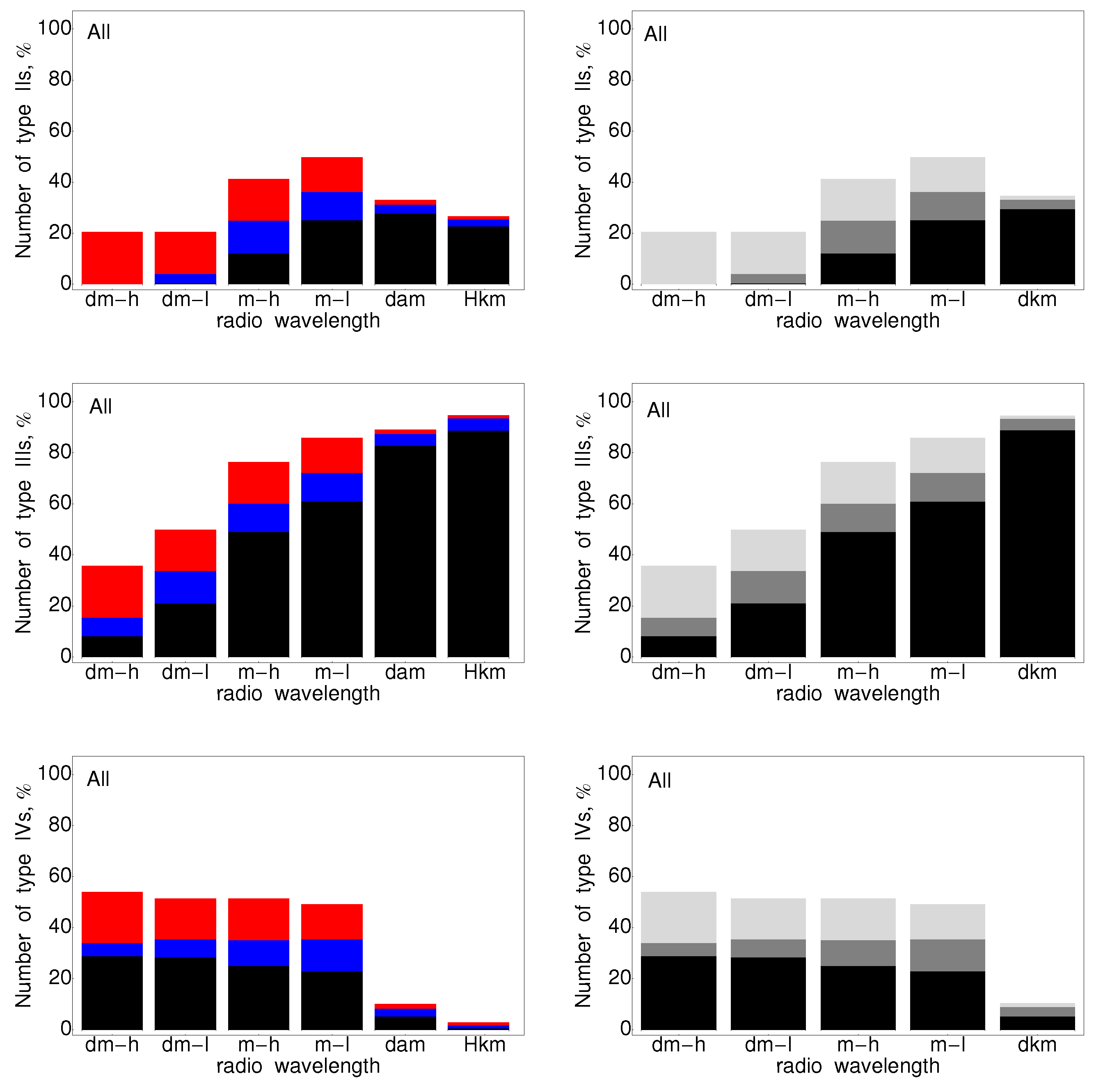
The dependencies of the SEE-related sample over the entire duration (two SCs) for types II, III and IV radio bursts are shown in Figure 1. On the left are organized the plots at all six frequency ranges given in color, and on the right are the histograms over the five bins in black-and-white. While comparing the two columns (for given radio burst type), we see that the tendencies in the first four bins are the same, whereas the trends between the IP bins are consistent between the left and right plots.
The top row shows the trends for the type II radio bursts, with a pronounced peak at m-l range (up to 36%, when combining the observed with reported/uncertain cases) and clear decline in the IP space. In the second row are presented the histograms for the type IIIs that show a steady rise of the occurrence with increase of radio wavelength reaching close to 100% in the IP space. The bottom row presents the behavior of the type IVs, from no pronounced trend as a function of frequency to a nearly complete lack of occurrence in the IP space. Although the number of visually observed events declines, if we add the uncertain and observatory reports, the sum (black and blue parts) is constant as a function of the frequency.
The numerical values of the results in the plots are summarized in Table 2 in normalized values, given in %. These are calculated as the ratio between the numbers, as given in parenthesis, to the entire event sample—832 events.
3.2. Solar Cycle Dependence
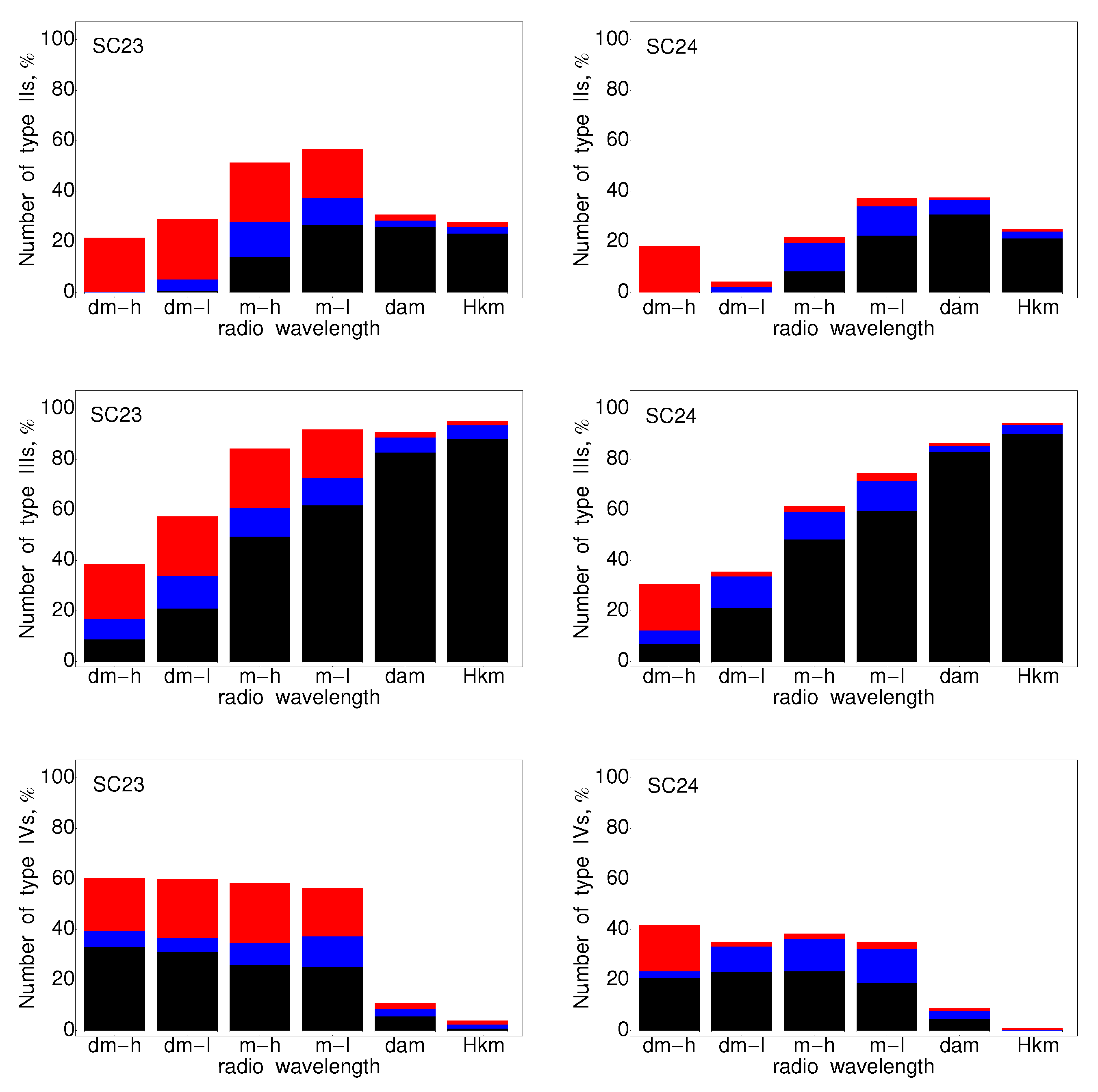
In this section, we focus on the intrinsic SC productivity of SEE events, by exploring the SC23 vs. SC24 trends of the occurrences of the three radio burst types as a function of the wavelength range, shown in Figure 2 and Table 3.
It has been known from previous works [51,54], that SC24 is weaker in activity (i.e., SFs, CMEs, SEPs, SEEs) compared to SC23. In order to eliminate the difference in the number of events in the given SC, each sample is normalized to its own size, SC23 to 547 and SC24 to 285 cases. Consistent overall trends are obtained between the two SCs (see Table 3 for the exact values), when the percentages of visual and uncertain cases are compared. Apart from the slight variations in individual wavelength ranges, e.g., (≲9%) of m-h IIs in SC23, dm-IVs and dam-IIs in SC24, no significant changes in the trends are evident from the distribution over the two SCs (compare with Figure 1 and Table 2). Thus, no excess SC productivity is found and the general radio burst trends as a function of the observed wavelength can be tabulated and used in future empirical studies. If all data gaps are uncovered and bursts happen to be found in each case, the weight of SC23 will increase. However, we consider such expectation of low probability.
The larger fraction of data gaps in SC23 (denoted with red color) can be regarded as another observational difference between the two SCs. As already discussed, this is mostly due to the lack of temporal coverage of the radio spectral data and the higher risk of unavailability for older data. This is especially true for the ground-based radio observatories, as the Wind/WAVES reports in the IP space are nearly complete due to the uninterrupted mode of space-borne observations.
The comparison of the trends when the two IP ranges are combined into a single bin can be inspected only from the tabulated results (and again denoted with ’dkm’ at the lowest row for each SC), see Table 3.
3.3. Longitudinal Dependence
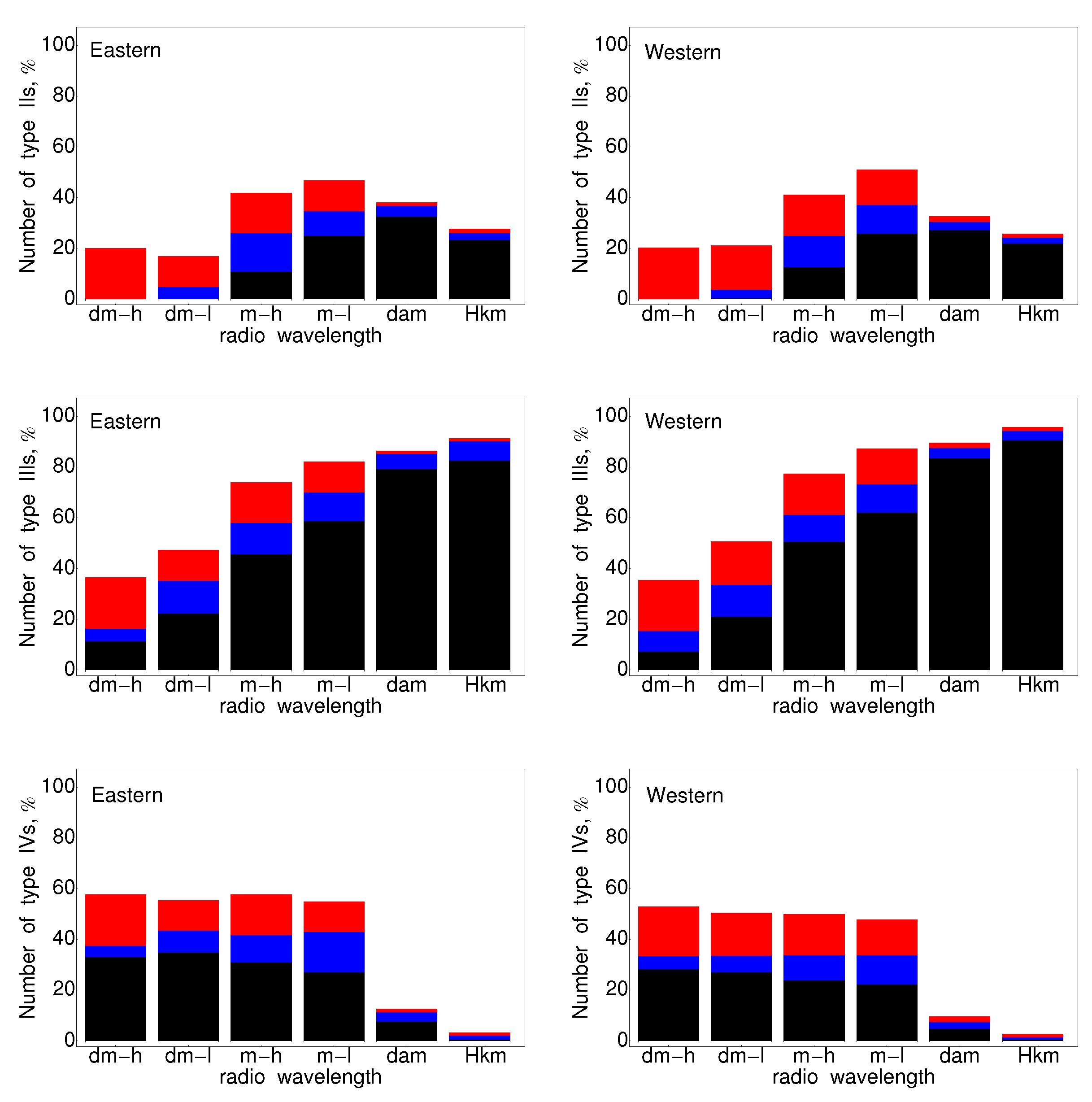
The dependence of the radio burst occurrences with respect to the helio-longitude of the SEE-associated solar origin is now considered. All histograms are given in Figure 3 for Eastern (on the left) and Western (on the right) longitudes. The exact numbers are summarized in this case in Table 4, see the first and fourth sections, respectively. For the quantitative comparison below, we use the sum of the first and second value of each column.
The results show that for Eastern type IIs, a slightly larger number is noticeable in the IP space (7% in both dam and Hkm-ranges), compared to the Western IIs. Similarly, larger fraction of Eastern type IVs can be recognized (≲10% in dm to m-ranges). No apparent differences (within few %) can be identified for type IIIs.
The helio-longitude distinction reflects the location of the SF/CME origin on the solar disk either as the reported active region (AR) longitude of the SF or the measurement position angle (MPA) of the CME. For the majority of cases, both give consistent results—each event can be readily identified either as Eastern or Western with 25/832 (3%) left with uncertain locations and thus will be dropped from this section. In the case of disk-center events, the MPA information is preferred, otherwise the AR reports are adopted.
As the analysis starts from in situ particle list, the longitudinal preference towards Western locations is intrinsic to the sample. Particle catalogs, e.g., [22,51], show that about 2/3 of the particle events originate from Western helio-longitudes. In order to exclude this bias, a normalization is needed. For the Eastern vs. Western trends, a division to 184 events (22%) in the former case and 623 (75%) in the latter is utilized. The proportion of data gaps is equally distributed from dm-h to m-l ranges, see the red blocks in Figure 3.
In addition, in Table 4, the values for the Eastern and Western events are explicitly given in each SC, although not shown as histograms. For example, ‘Eastern—All’ events are split into ‘Eastern—SC23’ and ‘Eastern—SC24’, however normalized to the total number of all Eastern events (184). Similarly, the SC-trends for the Western events are also shown in the last two sections of the table, normalized to 623 ‘Western—All’ events.
3.4. Electron Intensity Dependence
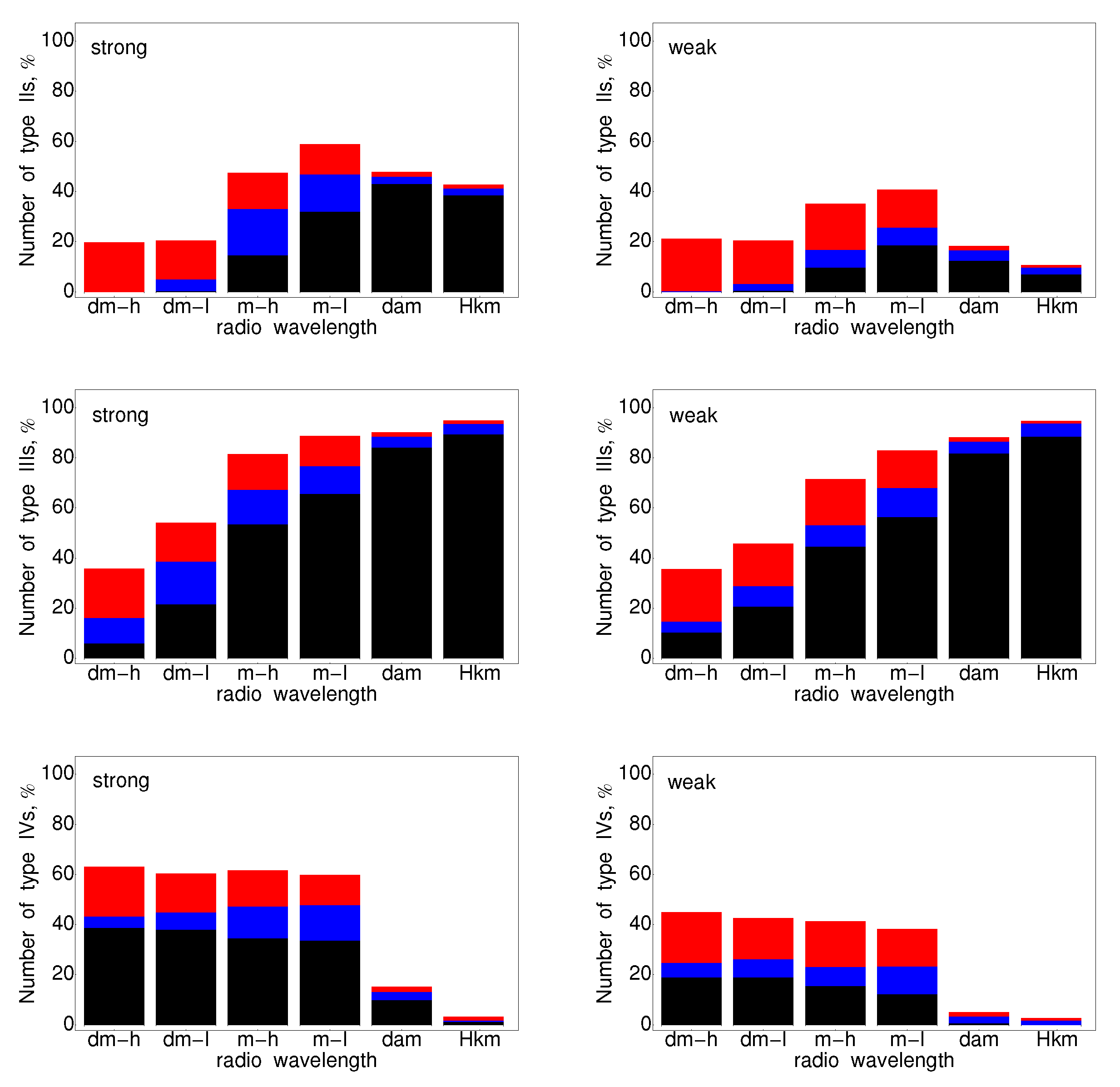
The strength of the solar activity is reflected in both the total number of events, but also in the frequency of manifestation of large or extreme solar phenomena. Here we explore the effect of the SEE amplitude solely on the number of observed radio bursts, as the radio intensity is not considered. We expect a marked difference in the numbers of the radio bursts, and the results are shown in Figure 4 and in Table 5.
The occurrence rate as a function of the electron intensity is investigated in view of the median value of the SEE events of the entire sample, calculated to be ∼507 differential electron flux units (DEFU)7. The sample is thus split into two parts, each containing 416 events and denoted as ’strong’, if the burst is associated with a SEE event with intensity larger than the median or ’weak’, in the opposite case.
The trends of the strong (on the left) and weak events (on the right) as a function of wavelength are shown in Figure 4. As expected, a reduction in the radio burst numbers is obtained for the weak-samples. Namely, a strong decline is clearly visible in the occurrences of type II and IV radio bursts, up to ∼30% and ∼25%, respectively, compared to the strong samples. In contrast, type IIIs show a moderate drop (≲10%) only for the dm-l and m-ranges.
Similarly for the Eastern and Western events, here also the values of the strong and weak cases are summarized in Table 5, for the entire sample (denoted with ’All’), and also for each sub-sample in SC23 and 24.
3.5. Flare and CME Trends with Radio Wavelength
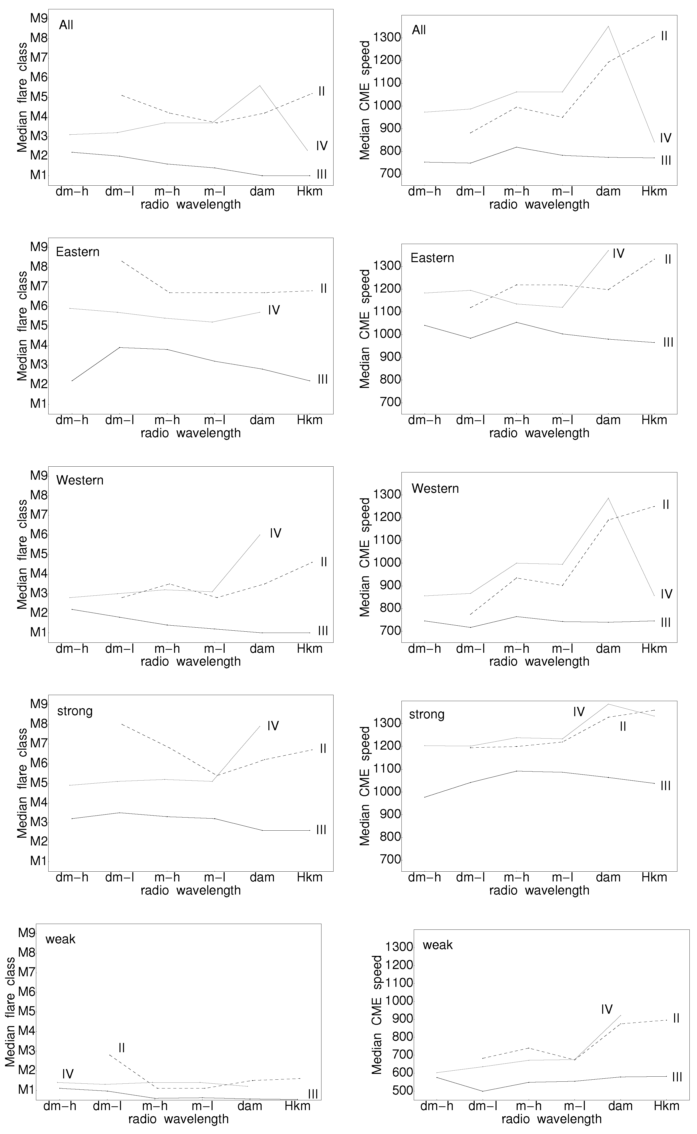
Similarly as in Paper I, we present also the effect of the solar origin strength on the radio burst presence in the different wavelength ranges. The intensity of the SFs and CMEs is quantified in terms of their SXR class and linear (and also projected on the sky) speed, respectively. For each wavelength range, we calculated the median value of the radio burst-associated SF class and CME speed and regard these as representative values for the solar origin. The dependencies of All, Eastern, Western, strong and weak sub-samples are shown in Figure 5. The trends for the SFs are shown on the left, and those for the CME speed—on the right. Three curves are depicted in each plot, for each of the considered burst types: dashed for the type IIs, solid black for the type IIIs and solid gray for type IVs.
Overall, after inspecting the individual plots, one concludes that the median values of SF and CME are lowest for the type III sample, whereas the type II and IV have closer values and exchange in the dominant position in the different groups. In addition, the type III trends are mostly flat, whereas the other two burst types often show rising dependency with wavelength increase (or alternatively with frequency decrease).
The Eastern trends have the larger median values compared to the Western (see second and third row of plots) for all burst types. This is true for both SF and CME parameters. The median values for the strong samples are in general larger compared to the weak samples (see the last two rows of plots), but also compared to the overall trends (top row). The strong samples have median values for the associated SF and CME comparable to the Eastern samples. The exact values can be inspected from Table 6.
3.6. On the Origin of SEE Events
The estimation on the SEE-origin (particle acceleration driven/dominated by SFs vs. CME-dominated) is done over the entire event sample and not as a function of wavelength. Following the requirement (for strict-to-relaxed preconditioning), as described in Paper I, we perform the similar calculations for the SEE-associated bursts types. Namely, we present the results in event numbers and percentages based on the total sample, 832, for the visual identifications and observatory reports. In the lower limit (or strict requirement), each accelerator is quantified in terms of radio burst occurrences over the entire wavelength range with a minimum possible contamination from the competing driver. In the upper limit (relaxed condition), the coverage of the radio burst type IIs and IIIs in the frequency domain can be partial. Contributions from type IV radio emission is not taken into account in the categorization below, also to be consistent with Paper I. From the entire event sample, for 14 events (or ≲2%) no radio signatures in any frequency range could be identified.
- Flare-dominated acceleration: The requirement in this case is to have type III bursts from low (or middle) corona up to IP space (with obligatory presence only in the Hkm range) and no presence of type II bursts at all times. Taking into account only the latter condition leads to a sub-sample of 270 events (32%), which is the theoretical upper limit for this category. The numbers of visual type IIIs (without overlap) from low corona to IP space are: dm-h-to-Hkm −20 (the extremely strict case); dm-l-to-Hkm −25; m-h-to-Hkm −74; m-l-to-Hkm −13; dam-to-Hkm −31; and Hkm only −14 (the extremely relaxed case), which sums to 177 cases (∼21%) altogether satisfying both conditions. If we also add the reported cases (in any of the frequency ranges), the total number increases to 241 (or 29%).
- CME-dominated acceleration: The demand for neither dm-h nor dm-l IIIs together with a condition for the occurrence of type IIs in any of the sub-bands over the dm-h-to-Hkm region leads to 148 cases (18%). Note that the strict condition of type II occurrence, namely a confirmed presence in the IP space, gives only 33 events.
- Mixed contribution: Whenever the above two constructs are violated, a mixed SF and CME influence to the SEE acceleration and thus to the radio burst is plausible. For the entire events sample, 143 cases (17%) fill in this mixed-category.
- Uncertain cases and data gaps: Whenever we cannot assuredly identify a burst type in any of the above sub-ranges, we select the event to fill in here (62 or 7%). In addition, we add all data gaps for type II and III (224 or 27%). Both requirements finally amount to 286 (or 34% out of all 832) events.
4. Discussion
This study explores the productivity of SEE-associated solar radio bursts of types II, III and IV for the entire duration of SCs 23 and 24. In order to exclude the bias towards sample sizes (any differences between the event numbers in regards to SC, helio-longitude and SEE amplitude), each occurrence is given in percentages, namely normalized to the number of events in the specific sub-group. The obtained results are roughly independent on SC. Type III radio burst occurrences are also consistent with respect to the longitude of their solar origin driver. The IP type IIs and dm-m IVs are more sensitive with respect to location, their Eastern samples being slightly more abundant (7–10%). The entire SEE sample was split equally to produce stronger and weaker than the median SEE-intensity samples, and the normalization was preformed for consistency with the other results. As expected, larger rates of occurrences were obtained in the case of strong samples, noticeably for type IIs and IVs in all wavelength ranges (as large as 25–30%, compared to the weak samples). Strong type III bursts, however, show up to 10% increases only in the dm and m ranges. Type IIIs are also easier to generate with respect to the other two burst types, since they are accompanied by SFs and CMEs with the lowest parameters within the sample. Type IIs and IV require stronger parent activity and thus are less frequent compared to the type IIIs with the exception of dm-IV. Additionally, the Eastern solar activity has larger values compared to the Western, when associated with SEEs. This is a well-known result and is explained with the requirement for stronger Eastern solar activity in order to compensate for the poor magnetic field line connection to Earth.
The previous reports on electron-associated radio bursts consider single events or small event samples, e.g., [24,25]. This is why a comparison with the proton-associated type II, III and IV radio bursts is performed instead (see numerous previous statistical studies as listed in [36,37], including Paper I, [38]). The overall trends between Paper I and the results presented here for type III and IV are consistent for all cases: All, Western, Eastern, strong and weak. The only difference is for the type IIs in the IP range, where for the SEP-association there is an increasing trend, whereas for the SEE-association there is a clear declining trend in all sub-groups, apart from the weak sample, where the SEP and SEE dependencies are the same. This finding inclines towards the interpretation that the IP IIs are proton-rich compared to the coronal IIs.
The strategy followed by the majority of studies on the temporal relationships between in situ particles and radio emission considers a comparison between the injection timing of particles and the shifted back to the Sun radio emission, e.g., [25,55]. Two different procedures are known, namely time shifting analysis and velocity dispersion analysis. Both impose certain assumptions, e.g., simultaneous acceleration at all energies in the solar corona and propagation in undisturbed IP space with Parker spiral-like magnetic field lines. Furthermore, no uncertainties are given on the deduced time of the particle release or the propagation path. Despite the implicit ambiguity, the obtained times are used to conclude on physical relationship or delayed acceleration between particles and radio emission signatures, e.g., [24,56].
An alternative reasoning is followed in this study, as proposed by Paper I. Namely, by either requiring or limiting the occurrences of given radio bursts in specific wavelength bands, one argues in favor of flare or CME predominance as the particle accelerator. For example, the exclusion of the CME-driven signatures at all times is used to estimate the fraction of flare-dominated electron sample. Similarly, excluding the events with flare-accelerated electron signatures in the low corona together with the demand of CME-driven emission is used to deduce the CME-dominated sample. This procedure can be regarded as an independent assessment on the solar origin of the electrons.
Following the above criteria, the flare-dominated origin of SEE events is found to be the primary acceleration mechanism for 29% of the electron sample, compared to 19% for the SEP events (as described in Paper I using consistent definitions). The opposite trend is obtained for the CME-dominated acceleration, with 18% for the electrons and 42% for the protons. A smaller fraction for the SEEs is also obtained in the Mixed category (17%) compared to SEPs (32%). Much larger numbers of data gaps and uncertain cases are found in the present study (34%) compared to a minor part of the SEP sample (7%) that compromises to some degree the precision of the above percentages. A complete reversal of the trends though is implausible, provided new dynamic spectra or observatory reports are recovered. Based on the data at hand, the different trends for the SF and CME driven categories support the histogram results for the smaller fraction of shock-related (in terms of type IIs) contribution to the electron case.
Finally, we compare the median properties of the SEE-associated SF and CME for the sub-groups under consideration. Exclusively, the median values for the type II (and IV) bursts are larger compared to the type III bursts for the entire sample and also with respect to helio-longitude or SEE-intensity. Only for the weak sample, the SF and CME values for all burst types are similar. While comparing the trends between the SEE and SEP samples, we obtain that for the proton-related type III case, SFs and CMEs have smaller, but comparable values, respectively. Type III radio bursts are much more frequent feature in the radio spectrum when we start from an electron list, and they do not seem to require a stronger parent eruption. Thus, type IIIs can be used as a proxy of electron acceleration, whereas type IIs need to be further explored as a possible proton-acceleration product.
The presented here results on the radio burst trends as a function of the wavelength of radio observation, helio-longitude and strength of the parent solar origin and on the particle amplitude itself, could be considered in the future development of empirical, multi-parametric schemes for SEE forecasting.
Supplementary Materials
The event list used in this work is available as supplementary material at https://0-www-mdpi-com.brum.beds.ac.uk/article/10.3390/universe8050275/s1. The extended version of the table will be released at: https://catalogs.astro.bas.bg/ (accessed on 1 May 2022).
Author Contributions
Conceptualization, R.M.; methodology, R.M.; software, R.M.; validation, R.M., S.W.S. and S.Z.; formal analysis, R.M. and S.W.S.; investigation, R.M., S.W.S. and S.Z.; resources, R.M., S.W.S. and S.Z.; writing—original draft preparation, R.M.; writing—review and editing, R.M., S.W.S. and S.Z.; visualization, R.M.; funding acquisition, R.M. All authors have read and agreed to the published version of the manuscript.
Funding
This research was funded by SCOSTEP/PRESTO 2020 grant ‘On the relationship between major space weather phenomena in solar cycles 23 and 24’.
Institutional Review Board Statement
Not applicable.
Informed Consent Statement
Not applicable.
Data Availability Statement
We gratefully acknowledge the open-source access to numerous catalogs, as outlined below: solar flare catalogs and information: ftp://ftp.ngdc.noaa.gov/STP/space-weather/solar-data/solar-features/solar-flares/x-rays/goes/ (accessed on1 May 2022), https://ftp.swpc.noaa.gov/pub/warehouse/ (accessed on 1 May 2022), https://solarmonitor.org/ (accessed on 1 May 2022); SOHO/LASCO CME catalog: https://cdaw.gsfc.nasa.gov/CME_list/ (accessed on 1 May 2022); Wind/EPACT proton catalog: http://newserver.stil.bas.bg/SEPcatalog/ (accessed on 1 May 2022); ACE/ EPAM electron catalog: https://www.nriag.sci.eg/ace_electron_catalog/ (accessed on 1 May 2022); Wind/WAVES radio emission from prepared videos: https://cdaw.gsfc.nasa.gov/CME_list/ (accessed on 1 May 2022); ground-based and space-borne dynamic radio spectra catalogs: http://www.asu.cas.cz/~radio/info.htm (accessed on 1 May 2022), https://sunbase.nict.go.jp/solar/denpa/index.html (accessed on 1 May 2022), https://www.sws.bom.gov.au/World_Data_Centre/1/9 (accessed on 1 May 2022), http://artemis-iv.phys.uoa.gr/Artemis4_list.html (accessed on 1 May 2022), http://soleil.i4ds.ch/solarradio/data/1998-2009_quickviews/ (accessed on 1 May 2022), http://secchirh.obspm.fr/ (accessed on 1 May 2022) (accessed on 1 May 2022), http://soleil.i4ds.ch/solarradio/callistoQuicklooks/ (accessed on 1 May 2022) (accessed on 1 May 2022), https://www.izmiran.ru/stp/lars/s_archiv.htm (accessed on 1 May 2022), https://www.sws.bom.gov.au/World_Data_Centre/1/9 (accessed on 1 May 2022), https://www.astro.umd.edu/~white/gb/index.shtml (accessed on 1 May 2022), https://solar-radio.gsfc.nasa.gov/wind/data_products.html (accessed on 1 May 2022), https://solar-radio.gsfc.nasa.gov/data/wind/ (accessed on 1 May 2022).
Conflicts of Interest
The authors declare no conflict of interest.
Abbreviations
The following abbreviations are used in this manuscript:
| AR | Active Region |
| CME | Coronal Mass Ejection |
| dam | decametric |
| dm | decimetric |
| H | hectometric |
| HXR | hard X-ray |
| II | type II solar radio burst |
| III | type III solar radio burst |
| IV | type IV solar radio burst |
| IP | Interplanetary |
| km | kilometric |
| m | metric |
| MPA | measurement position angle |
| SC | Solar Cycle |
| SEE | Solar Energetic Electron |
| SEP | Solar energetic Proton/Particle |
| SF | Solar Flare |
| SXR | soft X-ray |
| 1 | https://research.csiro.au/racs/home/gallery/a-sources/ (accessed on 1 May 2022). |
| 2 | https://www.nriag.sci.eg/ace_electron_catalog/ (accessed on 1 May 2022). |
| 3 | https://umbra.nascom.nasa.gov/goes/fits/ (accessed on 1 May 2022), https://data.nas.nasa.gov/helio/portals/solarflares/datasources.html (accessed on 1 May 2022). |
| 4 | https://cdaw.gsfc.nasa.gov/CME_list/ (accessed on 1 May 2022). |
| 5 | The Radio Solar Telescope Network (RSTN https://www.ngdc.noaa.gov/stp/space-weather/solar-data/solar-features/solar-radio/rstn-1-second/ (accessed on 1 May 2022)) at selected radio frequencies, is the only exception, for nearly complete UT coverage and long-duration solar radio observations with the similar radio instruments. |
| 6 | The decimetric (dm) and metric (m) bands are further split into high (h) and low (l) sub-ranges, whereas the Hectometric (H) and kilometric (km) are combined into one. |
| 7 | 1 DEFU = 1 electron/(cm sr sec keV). |
References
- Jansky, K.G. Radio Waves from Outside the Solar System. Nature 1933, 132, 66. [Google Scholar] [CrossRef]
- Warmuth, A.; Mann, G. The Application of Radio Diagnostics to the Study of the Solar Drivers of Space Weather. Lect. Notes Phys. 2004, 656, 49–68. [Google Scholar] [CrossRef]
- Ladreiter, H.P.; Zarka, P.; Lecacheux, A.; Macher, W.; Rucker, H.O.; Manning, R.; Gurnett, D.A.; Kurth, W.S. Analysis of electromagnetic wave direction finding performed by spaceborne antennas using singular-value decomposition techniques. Radio Sci. 1995, 30, 1699–1712. [Google Scholar] [CrossRef]
- Cecconi, B.; Bonnin, X.; Hoang, S.; Maksimovic, M.; Bale, S.D.; Bougeret, J.-L.; Goetz, K.; Lecacheux, A.; Reiner, M.J.; Rucker, H.O.; et al. STEREO/Waves Goniopolarimetry. Space Sci. Rev. 2008, 136, 549–563. [Google Scholar] [CrossRef]
- Martínez-Oliveros, J.C.; Lindsey, C.; Bale, S.D.; Krucker, S. Determination of Electromagnetic Source Direction as an Eigenvalue Problem. Sol. Phys. 2012, 279, 153–171. [Google Scholar] [CrossRef]
- Reiner, M.J.; Fainberg, J.; Kaiser, M.L.; Stone, R.G. Type III radio source located by Ulysses/Wind triangulation. J. Geophys. Res. 1998, 103, 1923–1932. [Google Scholar] [CrossRef]
- Thejappa, G.; MacDowall, R.J.; Bergamo, M. Emission Patterns of Solar Type III Radio Bursts: Stereoscopic Observations. Astrophys. J. 2012, 745, 187. [Google Scholar] [CrossRef]
- Krupar, V.; Santolik, O.; Cecconi, B.; Maksimovic, M.; Bonnin, X.; Panchenko, M.; Zaslavsky, A. Goniopolarimetric inversion using SVD: An application to type III radio bursts observed by STEREO. J. Geophys. Res. 2012, 117, A06101. [Google Scholar] [CrossRef]
- Krupar, V.; Maksimovic, M.; Santolik, O.; Cecconi, B.; Kruparova, O. Statistical Survey of Type III Radio Bursts at Long Wavelengths Observed by the Solar TErrestrial RElations Observatory (STEREO)/Waves Instruments: Goniopolarimetric Properties and Radio Source Locations. Sol. Phys. 2014, 289, 4633–4652. [Google Scholar] [CrossRef] [Green Version]
- Magdalenić, J.; Marqué, C.; Krupar, V.; Mierla, M.; Zhukov, A.N.; Rodriguez, L.; Maksimović, M.; Cecconi, B. Tracking the CME-driven Shock Wave on 2012 March 5 and Radio Triangulation of Associated Radio Emission. Astrophys. J. 2014, 791, 115. [Google Scholar] [CrossRef]
- Pick, M.; Vilmer, N. Sixty-five years of solar radioastronomy: Flares, coronal mass ejections and Sun Earth connection. AStronomy Astrophys. Rev. 2008, 16, 1–153. [Google Scholar] [CrossRef]
- Nindos, A.; Aurass, H.; Klein, K.L.; Trottet, G. Radio Emission of Flares and Coronal Mass Ejections. Invited Review. Sol. Phys. 2008, 253, 3–41. [Google Scholar] [CrossRef]
- Melrose, D.B. Coherent emission mechanisms in astrophysical plasmas. Rev. Mod. Plasma Phys. 2017, 1, 5. [Google Scholar] [CrossRef]
- Fletcher, L.; Dennis, B.R.; Hudson, H.S.; Krucker, S.; Phillips, K.; Veronig, A.; Battaglia, M.; Bone, L.; Caspi, A.; Chen, Q.; et al. An Observational Overview of Solar Flares. Space Sci. Rev. 2011, 159, 19–106. [Google Scholar] [CrossRef]
- Benz, A.O. Flare Observations. Living Rev. Sol. Phys. 2017, 14, 2. [Google Scholar] [CrossRef] [Green Version]
- Webb, D.F.; Howard, T.A. Coronal Mass Ejections: Observations. Living Rev. Sol. Phys. 2012, 9, 3. [Google Scholar] [CrossRef] [Green Version]
- Lin, R.P. Energetic solar electrons in the interplanetary medium. Sol. Phys. 1985, 100, 537–561. [Google Scholar] [CrossRef]
- Reid, H.A.S.; Ratcliffe, H. A review of solar type III radio bursts. Res. Astron. Astrophys. 2014, 14, 773. [Google Scholar] [CrossRef]
- Ratcliffe, H.; Kontar, E.P.; Reid, H.A.S. Large-scale simulations of solar type III radio bursts: Flux density, drift rate, duration, and bandwidth. Astron. Astrophys. 2014, 572, A111. [Google Scholar] [CrossRef]
- Cane, H.V.; Richardson, I.G.; von Rosenvinge, T.T. A study of solar energetic particle events of 1997-2006: Their composition and associations. J. Geophys. Res. 2010, 115, A08101. [Google Scholar] [CrossRef]
- Desai, M.; Giacalone, J. Large gradual solar energetic particle events. Living Rev. Sol. Phys. 2016, 13, 3. [Google Scholar] [CrossRef] [PubMed] [Green Version]
- Miteva, R.; Samwel, S.W.; Costa-Duarte, M.V. The Wind/EPACT Proton Event Catalog (1996–2016). Sol. Phys. 2018, 293, 27. [Google Scholar] [CrossRef] [Green Version]
- Ergun, R.E.; Larson, D.; Lin, R.P.; McFadden, J.P.; Carlson, C.W.; Anderson, K.A.; Muschietti, L.; McCarthy, M.; Parks, G.K.; Reme, H.; et al. Wind Spacecraft Observations of Solar Impulsive Electron Events Associated with Solar Type III Radio Bursts. Astrophys. J. 1998, 503, 435–445. [Google Scholar] [CrossRef]
- Krucker, S.; Larson, D.E.; Lin, R.P.; Thompson, B.J. On the Origin of Impulsive Electron Events Observed at 1 AU. Astrophys. J. 1999, 519, 864–875. [Google Scholar] [CrossRef]
- Lin, R.P. Relationship of solar flare accelerated particles to solar energetic particles (SEPs) observed in the interplanetary medium. Adv. Space Res. 2005, 35, 1857–1863. [Google Scholar] [CrossRef]
- Reid, H.A.S. A review of recent type III imaging spectroscopy. Front. Astron. Space Sci. 2020, 7, 56. [Google Scholar] [CrossRef]
- Vilmer, N.; MacKinnon, A.L.; Hurford, G.J. Properties of Energetic Ions in the Solar Atmosphere from Gamma-Ray and Neutron Observations. Space Sci. Rev. 2011, 159, 167–224. [Google Scholar] [CrossRef]
- Lysenko, A.L.; Frederiks, D.D.; Fleishman, G.D.; Aptekar, R.L.; Altyntsev, A.T.; Golenetskii, S.V.; Svinkin, D.S.; Ulanov, M.V.; Tsvetkova, A.E.; Ridnaia, A.V. X-ray and gamma-ray emission from solar flares. Phys. Uspekhi 2020, 163, 818–832. [Google Scholar] [CrossRef]
- Newkirk, G., Jr. The Solar Corona in Active Regions and the Thermal Origin of the Slowly Varying Component of Solar Radio Radiation. Astrophys. J. 1961, 133, 983. [Google Scholar] [CrossRef]
- Saito, K.; Makita, M.; Nishi, K.; Hata, S. A non-spherical axisymmetric model of the solar K corona of the minimum type. Ann. Tokyo Astron. Obs. 1970, 12, 51–173. [Google Scholar]
- Mann, G.; Jansen, F.; MacDowall, R.J.; Kaiser, M.L.; Stone, R.G. A heliospheric density model and type III radio bursts. Astron. Astrophys. 1999, 348, 614–620. [Google Scholar]
- Schwenn, R. Space Weather: The Solar Perspective. Living Rev. Sol. Phys. 2006, 3, 2. [Google Scholar] [CrossRef]
- Temmer, M. Space Weather: The Solar Perspective. Living Rev. Sol. Phys. 2021, 18, 4. [Google Scholar] [CrossRef]
- Pulkkinen, T. Space Weather: Terrestrial Perspective. Living Rev. Sol. Phys. 2007, 4, 1. [Google Scholar] [CrossRef] [Green Version]
- Wild, J.P.; Smerd, S.F.; Weiss, A.A. Solar Bursts. Astrophysics 1963, 1, 291. [Google Scholar] [CrossRef]
- Klein, K.-L. Radio astronomical tools for the study of solar energetic particles I. Correlations and diagnostics of impulsive acceleration and particle propagation. Front. Astron. Space Sci. 2021, 7, 105. [Google Scholar] [CrossRef]
- Klein, K.-L. Radio astronomical tools for the study of solar energetic particles II. Time-extended acceleration at subrelativistic and relativistic energies. Front. Astron. Space Sci. 2021, 7, 93. [Google Scholar] [CrossRef]
- Miteva, R.; Samwel, S.W.; Krupar, V. Solar energetic particles and radio burst emission. J. Space Weather. Space Clim. 2017, 7, A37. [Google Scholar] [CrossRef]
- Miteva, R.; Klein, K.-L.; Samwel, S.W.; Nindos, A.; Kouloumvakos, A.; Reid, H. Radio Signatures of Solar Energetic Particles During the 23rd Solar Cycle. Cent. Eur. Astrophys. Bull. 2013, 37, 541–553. [Google Scholar]
- Kahler, S.W. Radio burst characteristics of solar proton flares. Astrophys. J. 1982, 261, 710–719. [Google Scholar] [CrossRef]
- Cane, H.V.; Erickson, W.C.; Prestage, N.P. Solar flares, type III radio bursts, coronal mass ejections, and energetic particles. J. Geophys. Res. 2002, 107, 1315. [Google Scholar] [CrossRef] [Green Version]
- MacDowall, R.J.; Lara, A.; Manoharan, P.K.; Nitta, N.V.; Rosas, A.M.; Bougeret, J.L. Long-duration hectometric type III radio bursts and their association with solar energetic particle (SEP) events. Geophys. Res. Lett. 2003, 30, 8018. [Google Scholar] [CrossRef]
- Gopalswamy, N.; Yashiro, S.; Akiyama, S.; Mäkelä, P.; Xie, H.; Kaiser, M.L.; Howard, R.A.; Bougeret, J.L. Coronal mass ejections, type II radio bursts, and solar energetic particle events in the SOHO era. Ann. Geophys. 2008, 26, 3033–3047. [Google Scholar] [CrossRef]
- Winter, L.M.; Ledbetter, K. Type II and Type III Radio Bursts and their Correlation with Solar Energetic Proton Events. Astrophys. J. 2015, 809, 105. [Google Scholar] [CrossRef] [Green Version]
- Patel, B.D.; Joshi, B.; Cho, K.S.; Kim, R.S. DH Type II Radio Bursts During Solar Cycles 23 and 24: Frequency-Dependent Classification and Their Flare-CME Associations. Sol. Phys. 2021, 296, 142. [Google Scholar] [CrossRef]
- Heckman, G.R.; Kunches, J.M.; Allen, J.H. Prediction and evaluation of solar particle events based on precursor information. Adv. Space Res. 2020, 12, 313–320. [Google Scholar] [CrossRef]
- Núñez, M.; Paul-Pena, D. Predicting >10 MeV SEP Events from Solar Flare and Radio Burst Data. Universe 2020, 6, 161. [Google Scholar] [CrossRef]
- Kahler, S.W.; Cliver, E.W.; Ling, A.G. Validating the proton prediction system (PPS). J. Atmos. Sol.-Terr. Phys. 2007, 69, 43–49. [Google Scholar] [CrossRef]
- Laurenza, M.; Cliver, E.W.; Hewitt, J.; Storini, M.; Ling, A.G.; Balch, C.C.; Kaiser, M.L. A technique for short-term warning of solar energetic particle events based on flare location, flare size, and evidence of particle escape. Space Weather 2009, 7, S04008. [Google Scholar] [CrossRef] [Green Version]
- Zucca, P.; Núñez, M.; Klein, K. Exploring the potential of microwave diagnostics in SEP forecasting: The occurrence of SEP events. J. Space Weather Space Clim. 2017, 7, A13. [Google Scholar] [CrossRef]
- Samwel, S.W.; Miteva, R. Catalogue of in situ observed solar energetic electrons from ACE/EPAM instrument. Mon. Not. R. Astron. Soc. 2021, 505, 5212–5227. [Google Scholar] [CrossRef]
- Yashiro, S.; Gopalswamy, N.; Michalek, G.; St. Cyr, O.C.; Plunkett, S.P.; Rich, N.B.; Howard, R.A. A catalog of white light coronal mass ejections observed by the SOHO spacecraft. J. Geophys. Res. 2004, 109, A07105. [Google Scholar] [CrossRef]
- Miteva, R. On the solar origin of in situ observed energetic protons. Bulg. Astron. J. 2019, 31, 51. [Google Scholar]
- Miteva, R.; Samwel, S.W.; Costa-Duarte, M.V.; Malandraki, O.E. Solar cycle dependence of Wind/EPACT protons, solar flares and coronal mass ejections. Sun Geosph. 2017, 12, 11–19. [Google Scholar]
- Kouloumvakos, A.; Nindos, A.; Valtonen, E.; Alissandrakis, C.E.; Malandraki, O.; Tsitsipis, P.; Kontogeorgos, A.; Moussas, X.; Hillaris, A. Properties of solar energetic particle events inferred from their associated radio emission. Astron. Astrophys. 2015, 580, A80. [Google Scholar] [CrossRef] [Green Version]
- Haggerty, D.K.; Roelof, E.C. Impulsive Near-relativistic Solar Electron Events: Delayed Injection with Respect to Solar Electromagnetic Emission. Astrophys. J. 2002, 579, 841–853. [Google Scholar] [CrossRef]
Figure 1.
Plots of type II (top), III (middle) and IV (bottom) radio bursts for SC23 + 24 (denoted with ‘All’), normalized to 832 SEE events. For the color code see text.
Figure 1.
Plots of type II (top), III (middle) and IV (bottom) radio bursts for SC23 + 24 (denoted with ‘All’), normalized to 832 SEE events. For the color code see text.

Figure 2.
Plots of type II (top), III (middle) and IV (bottom) radio bursts, normalized to 547 SC23 (left) and 285 SC24 (on the right) SEE events. Color code as in Figure 1.
Figure 2.
Plots of type II (top), III (middle) and IV (bottom) radio bursts, normalized to 547 SC23 (left) and 285 SC24 (on the right) SEE events. Color code as in Figure 1.

Figure 3.
Plots of type II (top), III (middle) and IV (bottom) radio bursts, normalized to 184 Eastern (on the left) and 623 Western (on the right) SEE events. Color code as in Figure 1.
Figure 3.
Plots of type II (top), III (middle) and IV (bottom) radio bursts, normalized to 184 Eastern (on the left) and 623 Western (on the right) SEE events. Color code as in Figure 1.

Figure 4.
Plots of type II (top), III (middle) and IV (bottom) radio bursts for 416 strong (on the left), and 416 weak (on the right) in intensity SEE events. Color code as in Figure 1.
Figure 4.
Plots of type II (top), III (middle) and IV (bottom) radio bursts for 416 strong (on the left), and 416 weak (on the right) in intensity SEE events. Color code as in Figure 1.

Figure 5.
Plots of the wavelength dependency of the SF class (on the left) and CME speed (on the right) in median values. The sample type (All, Eastern, Western, strong or weak) and burst type (II, III and IV) are denoted in each plot.
Figure 5.
Plots of the wavelength dependency of the SF class (on the left) and CME speed (on the right) in median values. The sample type (All, Eastern, Western, strong or weak) and burst type (II, III and IV) are denoted in each plot.


Table 1.
A list with radio observatories, ground-based and space-borne used in the analysis.
| Archive/Radio | Frequency | Max UT | Yearly |
|---|---|---|---|
| Observatory | Coverage | Coverage | Coverage |
| Ondrejov | 0.8–5 GHz | 8–18 | 1991–now (selected) |
| http://www.asu.cas.cz/~radio/info.htm (accessed on 1 May 2022) | |||
| HiRAS | 25–2500 MHz | 18–12 | 1996–2016 |
| https://sunbase.nict.go.jp/solar/denpa/index.html (accessed on 1 May 2022) | |||
| Culgoora | 18–1800 MHz | 20–8 | 1992–now |
| https://www.sws.bom.gov.au/World_Data_Centre/1/9 (accessed on 1 May 2022) | |||
| ARTEMIS | 20–600 MHz | 5–16 | 1998–2013 (gaps) |
| http://artemis-iv.phys.uoa.gr/Artemis4_list.html (accessed on 1 May 2022) | |||
| Phoenix archive | various | various | 1978–2009 (gaps) |
| http://soleil.i4ds.ch/solarradio/data/1998-2009_quickviews/ (accessed on 1 May 2022) | |||
| Radio monitoring | various | 0–24 | 1997–now |
| http://secchirh.obspm.fr/ (accessed on 1 May 2022) | |||
| e-Callisto | various | various | 2002–now |
| http://soleil.i4ds.ch/solarradio/callistoQuicklooks/ (accessed on 1 May 2022) | |||
| Izmiran | 25–90 MHz | 6–12 | 2000–2019 |
| https://www.izmiran.ru/stp/lars/s_archiv.htm (accessed on 1 May 2022) | |||
| Learmonth | 25–180 MHz | 22–10 | 2000–now |
| https://www.sws.bom.gov.au/World_Data_Centre/1/9 (accessed on 1 May 2022) | |||
| Green Bank | 5–1100 MHz | 12–24 | 2004–2015 |
| https://www.astro.umd.edu/~white/gb/index.shtml (accessed on 1 May 2022) | |||
| Wind/WAVES | 20 kHz–14 MHz | 0–24 | 1994–now |
| https://solar-radio.gsfc.nasa.gov/wind/data_products.html (accessed on 1 May 2022) | |||
| https://solar-radio.gsfc.nasa.gov/data/wind/ (accessed on 1 May 2022) | |||
Table 2.
Table of the occurrence of radio burst types II, III and IV in the different wavelength ranges over the entire time period (All). The results are shown as: visually identified/uncertain associations with observatory reports/data gaps, in % and the exact numbers are given in parentheses. The round-off error is ≲1%. 100% corresponds to 832 events.
| Type | Type II | Type III | Type IV |
|---|---|---|---|
| All (832 cases) | |||
| dm-h | 0/0/20% (0/1/169) | 8/7/20% (68/60/169) | 29/5/20% (240/43/166) |
| dm-l | 0/4/16% (3/31/136) | 21/13/16% (176/105/169) | 28/7/16% (237/59/132) |
| m-h | 12/13/16% (101/97/136) | 49/11/16% (409/92/135) | 25/10/16% (209/84/135) |
| m-l | 25/11/13% (210/92/112) | 61/11/14% (508/94/112) | 23/13/14% (191/105/112) |
| dam | 28/3/1% (231/29/15) | 83/5/2% (508/94/112) | 5/3/2% (44/25/15) |
| Hkm | 23/3/1% (189/23/10) | 89/5/1% (740/39/10) | 1/1/1% (5/9/10) |
| dkm | 29/4/1% (246/31/11) | 89/4/1% (741/37/10) | 5/4/1% (44/31/11) |
Table 3.
Table of the occurrence of radio burst types II, III and IV in the different wavelength ranges for SC23 (normalized to 547 events) and SC24 (to 285, respectively). The results are shown as: visually identified/uncertain associations with observatory reports/data gaps, in % and the exact numbers are given in parentheses. The round-off error is ≲1%.
| Type | Type II | Type III | Type IV |
|---|---|---|---|
| SC23 (547 cases) | |||
| dm-h | 0/0/21% (0/1/117) | 1/8/21% (48/45/117) | 33/6/21% (181/35/114) |
| dm-l | 0/5/24% (3/25/130) | 21/13/24% (115/70/129) | 31/5/23% (171/30/127) |
| m-h | 14/14/24% (77/75/129) | 50/11/24% (271/61/129) | 26/8/24% (142/48/129) |
| m-l | 27/11/19% (146/59/104) | 62/11/19% (338/60/104) | 25/12/19% (137/67/104) |
| dam | 26/2/2% (143/13/12) | 83/6/2% (453/32/11) | 7/3/2% (31/16/12) |
| Hkm | 23/3/1% (128/15/8) | 88/5/1% (483/29/8) | 1/1/1% (5/8/8) |
| dkm | 28/3/2% (156/16/9) | 88/5/1% (484/28/8) | 6/4/2% (31/21/9) |
| SC24 (285 cases) | |||
| dm-h | 0/0/18% (0/0/52) | 7/5/18% (20/15/52) | 21/3/18% (59/8/52) |
| dm-l | 0/2/2% (0/6/6) | 21/12/2% (61/35/5) | 23/10/2% (66/29/5) |
| m-h | 8/11/2% (24/32/6) | 48/11/2% (138/31/6) | 24/13/2% (67/36/6) |
| m-l | 22/12/3% (64/33/8) | 60/12/3% (170/34/8) | 19/13/3% (54/38/8) |
| dam | 31/6/1% (88/16/3) | 83/2/1% (237/6/3) | 5/3/1% (13/9/3) |
| Hkm | 21/3/1% (61/8/2) | 90/4/1% (257/9/2) | 0/0/1% (0/1/2) |
| dkm | 32/5/1% (90/15/2) | 90/3/1% (257/9/2) | 5/4/1% (13/10/2) |
Table 4.
Table of the occurrence of radio burst types II, III and IV in the different wavelength ranges for Eastern and Western samples, for All, SC23 and SC24 time periods. The results are shown as: visually identified/uncertain associations with observatory reports/data gaps, in % and the exact numbers are given in parentheses. The round-off error is ≲1%.
| Type | Type II | Type III | Type IV |
|---|---|---|---|
| Eastern—All (184 cases) | |||
| dm-h | 0/0/20% (0/0/37) | 11/5/20% (21/9/37) | 33/4/20% (61/8/37) |
| dm-l | 0/5/12% (0/9/22) | 22/13/12% (41/24/22) | 35/9/12% (64/16/22) |
| m-h | 11/15/16% (20/28/29) | 46/13/16% (84/23/29) | 31/11/16% (57/20/29) |
| m-l | 25/10/12% (46/18/21) | 59/11/12% (108/21/21) | 27/16/12% (50/29/21) |
| dam | 33/4/1% (60/8/2) | 79/6/1% (146/11/2) | 8/4/1% (14/7/2) |
| Hkm | 27/4/2% (51/7/2) | 83/8/1% (152/14/2) | 1/2/1% (1/3/2) |
| dkm | 35/7/1% (64/12/2) | 83/8/1% (152/14/2) | 8/5/1% (14/9/2) |
| Eastern—SC23 (112 cases, normalized to All Eastern) | |||
| dm-h | 0/0/11% (0/0/21) | 8/3/11% (15/6/21) | 23/3/11% (42/6/21) |
| dm-l | 0/3/11% (0/6/21) | 13/10/11% (24/18/21) | 23/5/11% (42/9/21) |
| m-h | 8/11/15% (14/21/28) | 28/9/15% (52/16/28) | 18/7/15% (34/12/28) |
| m-l | 18/7/11% (33/13/20) | 37/7/11% (68/12/20) | 20/9/11% (36/17/20) |
| dam | 20/1/1% (36/1/1) | 48/5/1% (89/9/1) | 5/2/1% (9/4/1) |
| Hkm | 17/3/1% (32/5/1) | 49/7/1% (91/12/1) | 1/2/1% (1/3/1) |
| dkm | 21/3/1% (39/5/1) | 49/7/1% (91/12/1) | 5/3/1% (9/6/1) |
| Eastern—SC24 (72 cases, normalized to All Eastern) | |||
| dm-h | 0/0/9% (0/0/16) | 3/2/9% (6/3/16) | 10/1/9% (19/2/16) |
| dm-l | 0/2/1% (0/3/1) | 9/3/1% (17/6/1) | 12/4/1% (22/7/1) |
| m-h | 3/4/1% (6/7/1) | 17/4/1% (32/7/1) | 13/4/1% (23/8/1) |
| m-l | 7/3/1% (13/5/1) | 22/5/1% (40/9/1) | 8/7/1% (14/12/1) |
| dam | 13/4/1% (24/7/1) | 31/1/1% (57/2/1) | 3/2/1% (5/3/1) |
| Hkm | 10/1/1% (19/2/1) | 33/1/1% (61/2/1) | 0/0/1% (0/0/1) |
| dkm | 14/4/1% (25/7/1) | 33/1/1% (61/2/1) | 3/2/1% (5/3/1) |
| Western—All (623 cases) | |||
| dm-h | 0/0/20% (0/1/125) | 7/8/20% (46/50/125) | 28/5/20% (176/32/122) |
| dm-l | 0/3/17% (3/21/108) | 21/13/17% (131/79/106) | 27/7/17% (169/41/104) |
| m-h | 13/12/16% (79/77/100) | 51/11/16% (316/100/64) | 24/10/16% (149/62/100) |
| m-l | 26/11/14% (161/91/86) | 62/11/14% (387/69/86) | 22/12/14% (139/72/86) |
| dam | 27/3/2% (170/20/13) | 83/4/2% (520/26/12) | 5/3/2% (30/17/13) |
| Hkm | 22/2/1% (137/15/8) | 91/4/1% (564/24/8) | 1/1/1% (4/5/8) |
| dkm | 29/3/1% (181/18/9) | 91/4/1% (565/22/8) | 5/3/1% (30/21/9) |
| Western—SC23 (411 cases, normalized to All Western) | |||
| dm-h | 0/0/2% (0/0/14) | 5/6/14% (32/38/89) | 22/4/14% (136/26/86) |
| dm-l | 3/18/3% (0/3/17) | 14/8/16% (87/50/102) | 20/3/16% (125/19/100) |
| m-h | 10/8/15% (61/52/95) | 34/7/15% (210/42/95) | 17/5/15% (105/34/95) |
| m-l | 18/7/13% (110/43/79) | 41/7/13% (257/44/79) | 16/7/13% (99/46/79) |
| dam | 17/2/2% (106/11/11) | 55/4/2% (341/22/10) | 3/2/2% (22/11/11) |
| Hkm | 15/2/2% (95/9/7) | 59/3/1% (369/16/7) | 1/1/1% (4/4/7) |
| dkm | 19/2/1% (116/10/8) | 59/2/1% (370/15/7) | 4/2/1% (22/14/8) |
| Western—SC24 (212 cases, normalized to All Western) | |||
| dm-h | 0/0/6% (0/0/36) | 2/2/6% (14/12/36) | 6/1/6% (40/6/36) |
| dm-l | 0/0/1% (0/3/5) | 7/5/1% (44/29/4) | 7/4/1% (44/22/4) |
| m-h | 3/4/1% (18/25/5) | 17/4/1% (106/24/5) | 7/4/1% (44/28/5) |
| m-l | 8/4/1% (51/28/7) | 21/4/1% (130/25/7) | 6/4/1% (40/26/7) |
| dam | 10/1/0% (64/9/2) | 29/1/0% (195/8/1) | 1/1/0% (8/6/2) |
| Hkm | 7/1/0% (42/6/1) | 31/1/0% (195/8/1) | 0/0/0% (0/1/1) |
| dkm | 10/1/0% (65/9/1) | 31/1/0% (195/1/7) | 1/1/0% (8/7/1) |
Table 5.
Table of the occurrence of radio burst types II, III and IV in the different wavelength ranges for strong and weak SEE intensity, for All, SC23 and SC24 time periods. The results are shown as: visually identified/uncertain associations with observatory reports/data gaps, in % and the exact numbers are given in parentheses. The round-off error is ≲1%.
| Type | Type II | Type III | Type IV |
|---|---|---|---|
| Strong—All (416 cases) | |||
| dm-h | 0/0/20% (0/0/82) | 6/10/20% (25/42/82) | 39/5/20% (161/19/82) |
| dm-l | 0/5/15% (1/20/64) | 22/17/15% (90/71/64) | 38/7/15% (158/29/64) |
| m-h | 15/19/14% (61/77/59) | 54/14/14% (223/57/59) | 35/13/14% (144/53/59) |
| m-l | 32/15/12% (133/62/50) | 66/11/12% (273/46/50) | 35/13/14% (140/59/50) |
| dam | 43/3/2% (160/12/6) | 84/4/2% (350/18/7) | 10/3/2% (41/14/8) |
| Hkm | 39/3/1% (160/12/6) | 89/4/1% (372/17/6) | 1/0/1% (5/2/6) |
| dkm | 35/3/1% (190/10/7) | 89/4/1% (372/16/6) | 10/4/2% (41/16/7) |
| Strong—SC23 (289 cases, normalized to All strong) | |||
| dm-h | 0/0/14% (0/0/60) | 5/8/14% (20/32/60) | 30/4/14% (123/15/60) |
| dm-l | 0/4/15% (0/15/63) | 16/11/15% (65/36/63) | 28/4/15% (115/18/63) |
| m-h | 12/14/14% (49/57/58) | 38/10/14% (156/40/58) | 23/9/14% (96/36/58) |
| m-l | 23/11/12% (94/44/48) | 45/8/12% (186/35/48) | 23/10/11% (96/42/48) |
| dam | 29/1/1% (119/5/6) | 58/4/1% (243/16/5) | 7/2/1% (31/8/6) |
| Hkm | 27/1/1% (112/5/4) | 62/3/1% (259/11/4) | 1/0/1% (5/1/4) |
| dkm | 31/1/1% (128/4/5) | 62/3/1% (259/11/4) | 7/2/1% (31/9/5) |
| Strong—SC24 (127 cases, normalized to All strong) | |||
| dm-h | 0/0/5% (0/0/22) | 1/2/5% (5/10/22) | 9/1/5% (38/4/22) |
| dm-l | 0/1/0% (0/5/1) | 6/6/0% (25/25/1) | 10/3/0% (43/11/1) |
| m-h | 3/5/0% (12/20/1) | 16/4/0% (67/17/1) | 12/4/0% (48/17/1) |
| m-l | 9/4/1% (39/18/2) | 21/3/1% (87/11/2) | 11/4/1% (44/17/2) |
| dam | 14/2/1% (60/7/2) | 26/1/1% (102/2/2) | 2/1/1% (10/6/2) |
| Hkm | 12/2/1% (48/7/2) | 27/1/1% (113/6/2) | 0/0/1% (0/1/2) |
| dkm | 15/1/1% (62/6/2) | 27/1/1% (113/5/2) | 2/2/1% (10/7/2) |
| Weak—All (416 cases) | |||
| dm-h | 0/0/21% (0/1/87) | 10/4/21% (43/18/87) | 19/6/20% (79/24/84) |
| dm-l | 0/3/17% (2/11/72) | 21/8/17% (86/34/70) | 19/7/16% (79/30/68) |
| m-h | 10/7/18% (40/30/76) | 45/8/18% (186/35/76) | 16/7/18% (65/31/76) |
| m-l | 18/7/15% (77/30/62) | 56/12/15% (235/48/62) | 12/11/15% (51/46/62) |
| dam | 12/4/2% (52/17/7) | 82/5/2% (340/20/7) | 1/3/2% (3/11/7) |
| Hkm | 7/3/1% (29/11/4) | 88/5/1% (368/22/4) | 0/2/1% (0/7/4) |
| dkm | 13/51% (56/21/4) | 89/5/1% (369/21/4) | 1/4/1% (3/15/4) |
| Weak—SC23 (258 cases, normalized to All weak) | |||
| dm-h | 0/0/14% (0/1/57) | 7/3/14% (28/13/57) | 14/5/13% (58/20/54) |
| dm-l | 1/2/16% (2/10/67) | 12/6/16% (50/24/66) | 13/3/15% (56/12/64) |
| m-h | 7/4/17% (28/18/71) | 28/5/17% (115/21/71) | 11/3/17% (46/12/71) |
| m-l | 13/4/13% (52/15/56) | 36/6/13% (152/25/56) | 10/6/13% (41/25/56) |
| dam | 6/2/1% (24/8/6) | 50/4/1% (210/16/6) | 1/2/1% (0/8/6) |
| Hkm | 4/2/1% (16/10/4) | 54/4/1% (224/18/4) | 0/2/1% (0/7/4) |
| dkm | 7/3/1% (28/12/4) | 54/4/1% (225/17/4) | 1/3/1% (0/15/4) |
| Weak—SC24 (158 cases, normalized to All weak) | |||
| dm-h | 0/0/7% (0/0/30) | 4/1/7% (15/5/30) | 5/1/7% (21/4/30) |
| dm-l | 0/0/1% (0/1/5) | 9/2/1% (36/10/4) | 6/4/1% (23/18/4) |
| m-h | 3/3/1% (12/12/5) | 17/3/1% (71/14/5) | 5/5/1% (19/19/5) |
| m-l | 6/4/1% (25/15/6) | 20/6/1% (83/23/6) | 2/5/1% (10/21/6) |
| dam | 7/2/0% (28/9/1) | 31/1/0% (130/4/1) | 1/1/0% (3/3/1) |
| Hkm | 3/0/0% (13/1/0) | 35/1/0% (144/4/0)) | 0/0/0% (0/0/0) |
| dkm | 7/2/0% (28/9/0) | 35/1/0% (144/4/0) | 1/1/0% (3/3/0) |
Table 6.
Table of the median values of SFs/CMEs for All, Eastern, Western, strong and weak samples. The flare is given in SXR class and the CMEs are given in linear speed (km s). The exact size of each sample is given in parentheses.
Table 6.
Table of the median values of SFs/CMEs for All, Eastern, Western, strong and weak samples. The flare is given in SXR class and the CMEs are given in linear speed (km s). The exact size of each sample is given in parentheses.
| Type | Type II | Type III | Type IV |
|---|---|---|---|
| All | |||
| dm-h | − (1)/− (1) | M2.2 (121)/753 (106) | M3.1 (261)/973 (247) |
| dm-l | M5.1 (32)/882 (31) | M2.0 (252)/749 (239) | M3.2 (272)/987 (261) |
| m-h | M4.2 (191)/995 (188) | M1.6 (431)/819 (439) | M3.7 (267)/1062 (268) |
| m-l | M3.7 (268)/950 (274) | M1.4 (493)/783 (524) | M3.7 (296)/1062 (266) |
| dam | M4.2 (217)/1193 (248) | M1.0 (580)/774 (624) | M5.6 (60)/1351 (64) |
| Hkm | M5.2 (178)/1306 (200) | M1.0 (599)/772 (669) | M2.3 (7)/842 (12) |
| dkm | M4.0 (277)/1151 (263) | M1.0 (598)/772 (669) | M5.0 (63)/1306 (69) |
| Eastern | |||
| dm-h | − (0)/− (0) | M2.2 (29)/1041 (23) | M5.9 (64)/1183 (58) |
| dm-l | M8.3 (9)/1119 (9) | M3.9 (59)/984 (53) | M5.7 (73)/1195 (67) |
| m-h | M6.7 (46)/1219 (40) | M3.8 (93)/1054 (93) | M5.4 (71)/1135 (70) |
| m-l | M6.7 (59)/1219 (54) | M3.2 (103)/1003 (108) | M5.2 (75)/1120 (68) |
| dam | M6.7 (57)/1198 (64) | M2.8 (118)/980 (136) | M5.7 (19)/1370 (20) |
| Hkm | M6.8 (51)/1332 (58) | M2.2 (121)/965 (144) | − (2)/− (3) |
| dkm | M6.5 (63)/1198 (76) | M2.2 (121)/965 (144) | M5.3 (20)/1366 (21) |
| Western | |||
| dm-h | − (1)/− (1) | M2.2 (90)/1041 (23) | M2.8 (191)/856 (189) |
| dm-l | M2.8 (22)/775 (22) | M1.8 (187)/717 (186) | M3.0 (193)/867 (194) |
| m-h | M3.5 (141)/935 (148) | M1.4 (326)/765 (346) | M3.2 (191)/1000 (198) |
| m-l | M2.8 (203)/902 (220) | M1.2 (373)/743 (416) | M3.1 (188)/995 (198) |
| dam | M3.5 (158)/1190 (184) | M1.0 (437)/740 (488) | M6.0 (40)/1286 (44) |
| Hkm | M4.5 (125)/1250 (148) | M1.0 (453)/746 (525) | M2.8 (4)/857 (9) |
| dkm | M3.3 (164)/1138 (193) | M1.0 (452)/746 (525) | M5.3 (42)/1216 (48) |
| strong | |||
| dm-h | − (0)/− (0) | M3.2 (63)/977 (58) | M4.9 (170)/1203 (165) |
| dm-l | M8.0 (19)/1194 (21) | M3.5 (143)/1042 (145) | M5.1 (173)/1201 (174) |
| m-h | M6.8 (131)/1199 (129) | M3.3 (246)/1092 (255) | M5.2 (181)/1238 (186) |
| m-l | M5.4 (173)/1219 (180) | M3.2 (264)/1087 (287) | M5.1 (199)/1233 (188) |
| dam | M6.2 (168)/1328 (183) | M2.6 (304)/1064 (325) | M7.9 (50)/1386 (54) |
| Hkm | M6.7 (153)/1359 (164) | M2.6 (312)/1038 (324) | M3.5 (5)/1333 (7) |
| dkm | M5.8 (174)/1307 (192) | M2.6 (311)/1038 (342) | M7.9 (51)/1376 (56) |
| weak | |||
| dm-h | − (0)/− (0) | M1.1 (58)/576 (48) | M1.4 (91)/603 (82) |
| dm-l | M2.8 (13)/683 (10) | C9.6 (109)/499 (94) | M1.3 (99)/636 (87) |
| m-h | M1.1 (60)/740 (59) | C5.9 (185)/549 (184) | M1.4 (86)/672 (82) |
| m-l | M1.1 (95)/674 (94) | C6.2 (229)/555 (237) | M1.4 (87)/676 (78) |
| dam | M1.5 (49)/875 (65) | C5.6 (276)/579 (299) | M1.2 (10)/922 (10) |
| Hkm | M1.6 (25)/896 (36) | C5.3 (287)/582 (327) | − (2)/− (5) |
| dkm | M1.5 (55)/832 (71) | C5.3 (287)/582 (327) | M1.1 (12)/827 (13) |
Publisher’s Note: MDPI stays neutral with regard to jurisdictional claims in published maps and institutional affiliations. |
© 2022 by the authors. Licensee MDPI, Basel, Switzerland. This article is an open access article distributed under the terms and conditions of the Creative Commons Attribution (CC BY) license (https://creativecommons.org/licenses/by/4.0/).
Share and Cite
MDPI and ACS Style
Miteva, R.; Samwel, S.W.; Zabunov, S. Solar Radio Bursts Associated with In Situ Detected Energetic Electrons in Solar Cycles 23 and 24. Universe 2022, 8, 275. https://0-doi-org.brum.beds.ac.uk/10.3390/universe8050275
AMA Style
Miteva R, Samwel SW, Zabunov S. Solar Radio Bursts Associated with In Situ Detected Energetic Electrons in Solar Cycles 23 and 24. Universe. 2022; 8(5):275. https://0-doi-org.brum.beds.ac.uk/10.3390/universe8050275
Chicago/Turabian StyleMiteva, Rositsa, Susan W. Samwel, and Svetoslav Zabunov. 2022. "Solar Radio Bursts Associated with In Situ Detected Energetic Electrons in Solar Cycles 23 and 24" Universe 8, no. 5: 275. https://0-doi-org.brum.beds.ac.uk/10.3390/universe8050275
Note that from the first issue of 2016, this journal uses article numbers instead of page numbers. See further details here.