
Topological Gauge Actions on the Lattice as Overlap Fermion Determinants

1
Department of Physics, College of William & Mary, Williamsburg, VA 23185, USA
2
Thomas Jefferson National Accelerator Facility, Newport News, VA 23606, USA
3
Department of Physics, Florida International University, Miami, FL 33199, USA
*
Authors to whom correspondence should be addressed.
Universe 2022, 8(6), 332; https://0-doi-org.brum.beds.ac.uk/10.3390/universe8060332
Submission received: 10 April 2022
/
Revised: 31 May 2022
/
Accepted: 10 June 2022
/
Published: 17 June 2022
(This article belongs to the Special Issue Numerical Studies of Strongly Coupled Gauge Theories (SCGTs) in the Search of New Physics)
Abstract
:Overlap fermion on the lattice has been shown to properly reproduce topological aspects of gauge fields. In this paper, we review the derivation of Overlap fermion formalism in a torus of three space-time dimensions. Using the formalism, we show how to use the Overlap fermion determinants in the massless and infinite mass limits to construct different continuum topological gauge actions, such as the level-k Chern–Simons action, “half-CS” term and the mixed Chern–Simons (BF) coupling, in a gauge-invariant lattice UV regulated manner. Taking special Abelian and non-Abelian background fields, we demonstrate numerically how the lattice formalism beautifully reproduces the continuum expectations, such as the flow of action under large gauge transformations.
1. Introduction
The gauge theories in three space-time dimensions admit a parity-odd Chern–Simons (CS) topological gauge action in addition to the parity-even Maxwell gauge action. The Maxwell theory can be nonperturbatively regulated via the lattice discretization of space-time and by using the local plaquette gauge action. The CS theories are not so straightforward to regulate on the lattice, mainly due to the fact that the CS action is only gauge-invariant up to integer winding under nontrivial gauge transformations (e.g., [1]) and it is not possible to realize such a term simply as a local Wilson loop gauge action. Vigorous research work is being conducted on CS theories coupled to matter content and certain infrared duality relations [2,3,4] have been conjectured to exist at critical points separating different topological phases. Therefore, the question of how to study such theories numerically on the lattice is important. The aim of this paper is to elucidate how to introduce topological gauge actions, such as the Chern–Simons action, on the lattice in a completely gauge-invariant manner by identifying such actions as the induced gauge actions of lattice fermions.
Let us first consider gauge theories in even dimensions to see how gauge field topology is realized using lattice fermions. The space of Euclidean continuum gauge fields, , in even dimensional space, , usually has infinitely many disconnected pieces and each piece has an associated topological number. This is well known and a chapter or more is attributed to this topic in all modern books on quantum field theory; we find it useful to refer to the lecture notes by Bilal [5] which has a complete self-contained description and has citations to other relevant lecture notes and books. The topological number is given by
where is the Euclidean field strength associated with and . As such not all gauge fields can be connected to the trivial one, . One way to nonperturbatively regularize a gauge theory is using lattice, where one introduces gauge fields via gauge-links that connect neighboring lattice sites. Link variables belonging to the Lie group defined by the path ordered product of the Lie group elements,
along the path connecting x and (we have set the lattice spacing to unity and x takes on integer values) are lattice gauge fields. Naively, for some real valued parameter q, continuously connects any gauge field configuration on the lattice to the trivial one, , by sliding the value of q from 0 to 1 seemingly without encountering any singular behavior in gauge-links or the plaquettes at any x during the process. Notwithstanding the apparent lack of discontinuity on the lattice between any two gauge-fields that could otherwise be topologically distinct from each other in the continuum, an assignment of a topological integer to every gauge field configuration is still possible. A straightforward approach is to invoke the Atiyah–Singer index theorem [6] and use fermions to match Q with the index of a lattice Dirac operator. For every lattice gauge field background in even dimensions and the associated massive Hermitian Wilson–Dirac operator, , the index is the difference between the total number of negative eigenvalues of [7]. If the index associated with a particular, is not zero, we will see an eigenvalue of cross zero as one smoothly changes in . Therefore, there is one value of q where the ground state of the many body operator
for a dimensional auxiliary fermionic system, with , a being canonical fermion creation and annihilation operators, is doubly degenerate. As is also well known, chiral gauge anomalies in even dimensions are closely related to the topological index [5] and this can also be understood in terms of the ground state, , of as explained in [8]. Having defined the one form,
it is shown in [8] that
is a well defined function of the lattice gauge field background and and are the consistent and covariant currents. The problem of anomaly cancellation can be studied using Equation (5) and the need to fine tune the lattice Wilson–Dirac operator is discussed in [8]. The above discussion on the ability of massless overlap fermion to detect and classify topologically distinct gauge sectors on the lattice is well-known. In this paper, we review the aspects of overlap fermions in odd-dimensions, especially in 2 + 1 dimensions, and how the parity anomaly of overlap fermions can be used to introduce topological gauge actions that are characteristic of odd-dimensional gauge theories.
Chiral anomaly inducing topological index in even dimensions and parity anomaly inducing the Chern–Simons action in odd-dimensions are locally related as [5]
where is the Chern–Simons form in one dimension lower, namely, . Setting a one-parameter family of gauge fields equal to , and noting that ,
Focusing on , we have
Similar to our discussion on the challenge in defining the topological index simply as a local operator constructed out of local Wilson-loop operators on the lattice, it is not simple to define the above Chern–Simons form as a local gauge-link-based operator and be able to satisfy invariance under large gauge transformations of the type we will discuss later in this paper. Solution to this problem again is to introduce the Chern–Simons action using the fermions on the lattice; concretely, through the parity-odd part of the induced gauge action from overlap fermions. An early study in Ref. [9] showed that the Abelian parity anomaly is reproduced using lattice perturbation theory with a single-flavor of two-component Wilson fermion with non-zero mass at lattice UV scales [9]. The important point we stress in this paper is that the massive two-component Wilson Dirac operator X on any background field , immediately leads to a gauge covariant unitary operator [10], V,
and the gauge-invariant phase of is parity-odd and becomes the lattice realization of the Chern–Simons action for any gauge field background [10,11,12,13]. The unitary operator V is nothing but the overlap operator of a two-component fermion of mass of inverse lattice spacing. The phase within lattice regularization has been extensively analyzed in [14] for various Abelian backgrounds. In addition to the Chern–Simons action, the recent literature on fractional quantum Hall states rely heavily on parity-anomalous two-component exactly massless Dirac fermions that leads to the so-called “half-Chern–Simons” term. Subtleties arise when discussing half the Chern–Simons action while maintaining gauge invariance [2,15,16]. We also show how the construction of the unitary lattice operator V also immediately leads to the generalization of the Chern–Simons term to include the BF terms such as .
In order to keep this paper as self-contained as possible, we first review the derivation and the salient features of overlap fermions in three dimensions in Section 2. In Section 3, we focus on the variation of overlap fermion determinant as fermion mass is varied from to massless limit; the point of this discussion is to show that the infinite mass and zero fermion mass limits indeed correctly reproduce the Chern–Simons and “half-Chern–Simons” terms correctly in the continuum limit and independent of any lattice UV regulator parameters, such as the mass term in the Wilson fermion kernel. More interestingly, in Section 4, we take specific Abelian backgrounds with non-trivial topology on 2d spatial planes and show how the flow from infinite mass to zero mass limit preserves gauge invariance. For this, we follow the discussion in [10]. In Section 5, we take a non-Abelian background to discuss how the part of CS term present for non-Abelian case is correctly reproduced. After the discussion of the Chern–Simons terms, in Section 6, we focus on straight-forward extensions of overlap formalism to implement mixed Chern–Simons terms that couple two different gauge field backgrounds, and as a consequence, provide dictionary between some of the recently proposed fermion-boson dualities in the continuum to those on the lattice.
2. Overlap Formalism in Three Dimensions
This section follows [17] very closely and we repeat the derivation while keeping a phase ambiguity intact till the very end. Despite this paper being about nonperturbative regularization of topological field theories, the lattice formalism is strictly presented on toroidal manifold tessellated into uniform cubes of volume , with a being the lattice spacing. The naïve massless Dirac operator on a three dimensional lattice (we will set the lattice spacing to unity) is given by
where are Pauli matrices satisfying , and the action of translation operator up to lattice periodicity. Under parity (),
and under a gauge transformation ,
which implies
The naïve massless Dirac operator has a two fold degeneracy in all gauge field backgrounds. Furthermore, for every eigenvalue there is one with the opposite sign. To see these two features, we observe that the anti-Hermitian operator only couples odd lattice sites with even lattice sites. The eigenvalues come in pairs and the fermion determinant is real and positive in all gauge backgrounds and there is no parity anomaly. In order to realize a single flavor two-component massive Dirac fermion without any doublers in the overlap formalism [7], we define two Hamiltonians that act on four component spinors:
where 1 denotes an identity matrix of the same size as D. We have added the Wilson term,
with a Wilson mass parameter and under parity. Under a gauge transformation
Define the many body Hamiltonians by
with and being canonical creation and annihilation operators for fermions. With denoting the ground states of , the generating functional for a single two-component overlap fermion with a mass, m, is
where are Grassmann variables.
The problem of diagonalizing in three dimensions is simplified by going to a new basis. Let
The rotated Hamiltonian is
We can write
We define the unitary operator as
and does not suffer from the phase ambiguity present in R (L is fixed once R is fixed). Under parity,
and under a gauge transformation
Let us make the dependence of V on U explicit and derive the relation under charge conjugation ():
We first note that
From this we obtain
and our relation, Equation (25), follows.
We can diagonalize as
We define new sets of canonical creation and annihilation operators by
and we can write
The ground states, , are obtained by filling all the states corresponding to and , respectively. Therefore, we have
Using the above equations, we can write
where
Since
it follows that
Therefore, we have
The fermion mass is in the range and the fermion determinant is gauge invariant. There is a phase ambiguity present in the fermion determinant due to and the fermion determinant at is . The choice of fixing this phase is tied to the choice of preserving parity symmetry at at the cost of introducing gauge anomaly, and the choice of preserving gauge invariance at the cost of losing parity symmetry at . For the latter option, the choice of fixes the phase of infinite mass, , fermion and preserves gauge invariance for all values of m. In this paper, we will set from here on.
3. Introducing Chern–Simons and Half-Chern–Simons Terms on the Lattice
With the choice of phase as explained in the last section, the fermion determinant becomes
and it satisfies
This is the parity anomaly which has the built in feature that if we write
then
and is usually written using the -invariant as (Note, the propagator satisfies and preserve parity. Thus the anomaly is in the fermion induced gauge measure.) With this lattice formalism, we have all the required ingredients for constructing Chern–Simons theories on lattice by the identification of the parity-odd phase of with level-1 Chern–Simons action. As the simplest case, we can introduce a level-k Chern–Simons action as
In the massless limit, it is easy to see that the phase of is half of up to . We can introduce the so-called “half-Chern–Simons” theories on the lattice as
First, how do we know that is the same as Chern–Simons term? In the study in [9], it is analytically shown that the phase of in the massive Wilson fermion case is the same as Chern–Simons term. The pure phase in the case of overlap fermions is the same as the phase of , and, hence, we can borrow their results for overlap fermions. In the subsequent two sections, we will also take an empirical approach and show that for cases of Abelian and non-Abelian background fields where Chern–Simons term can be exactly be worked out, the phase indeed approaches the expectations in the continuum limit. Second, how did we manage to introduce “half-Chern–Simons” term in an evidently gauge-invariant manner? Using a non-trivial Abelian background in the next section, we demonstrate this through the flow of the phase of massless overlap fermion determinant as a function of the Wilson loop, for , and show that at specific where there is a discontinuity in the phase at , the determinant also vanishes.
4. Fermion Determinant in an Abelian Background with Uniform Magnetic Flux and Non-Trivial Temporal Wilson Loop
We now analyze the complex fermion determinant of a two-component three dimensional fermion in a well known Abelian background of interest both from the view point of showing subtle properties under gauge invariance and also from its relevance in condensed matter physics [2]. The gauge field background on a continuum torus is
Since has to be gauge equivalent to , Q has to be an integer. In addition, gauge invariance sets all to be equivalent for any integer n. The evaluation of the Chern–Simons action for this background in Equation (45) is tricky [16] and yields
Since , for this background, Q is the topological charge in all two-dimensional slices at a fixed and the deformation of A to has to connect two dimensional gauge fields in disconnected spaces. With a lattice regularization, , as t goes from , will result in Q levels of the two dimensional Wilson–Dirac operator crossing zero [14] and the phase within lattice regularization properly reproduces the gauge invariant Chern–Simons action [14]. Overlap fermions can be used to study the complex fermion determinant strictly in the massless limit with the lattice regularization in place and we will show that the massless fermion determinant has a zero in the path connecting and for a fixed Q enabling it to correctly reproduce (1) a smooth function of , (2) that is gauge invariant under , (3) equal to half of in Equation (46) at all values of , and (4) has a jump in the phase at the location of the zero of the fermion determinant.
We can implement the above Abelian background on the lattice by using the gauge-links as
on a three dimensional periodic lattice defined by the points and
Only the plaquettes in the plane have a non-zero flux and they are given by
We note that the flux is not uniform and singular in the continuum limit if Q is not an integer. Therefore, we will set Q to be integers.
Since the gauge field background does not depend on , one can go to momentum space in this direction. We will assume fermions obey antiperiodic boundary conditions in this direction. Setting these momenta to be , , the operators B and D reduce to
with the gauge fields in the (1-2) plane being and . Let us denote the fermion determinant by on the periodic lattice in this background and note that
We define
and
as the determinant with reference to and the determinant at with respect to the free determinant, respectively and is a real function. The key properties of the overlap fermion determinant are shown in the figures from Figure 1, Figure 2, Figure 3, Figure 4 and Figure 5. Let us start with the top panel of Figure 1 which focuses on the Chern–Simons action, namely, . We have shown the results only for but the limit is independent of and we should find
The top panel clearly shows that the correct limit is approached for as ( and fall on top of each other) and the dependence on Q is also as expected and the overlap fermion correctly reproduces the first subtle properly and this is an obvious consequence of the same result with Wilson fermions seen in [14]. We move on to behavior of the phase for the massless fermions in the bottom panel of Figure 1. We should find
and
This necessitates a jump in the phase when the flux quantum, Q, takes on odd values. First of all, we see that the phase has a limit when as seen by comparing the behavior for and . Furthermore, the results for and are indistinguishable from showing the independence on the regulator parameter, , as . Finally, we see that the phase shows a jump of at for and .
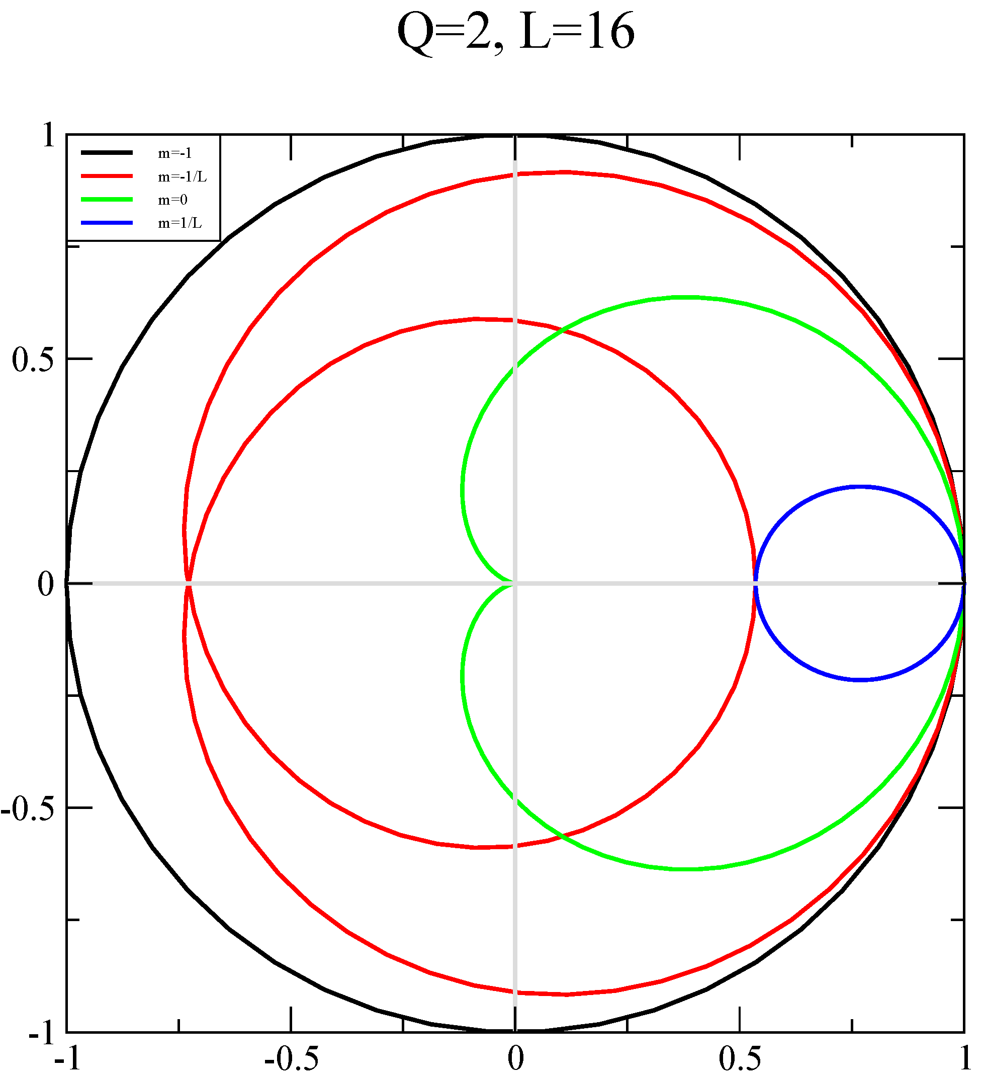
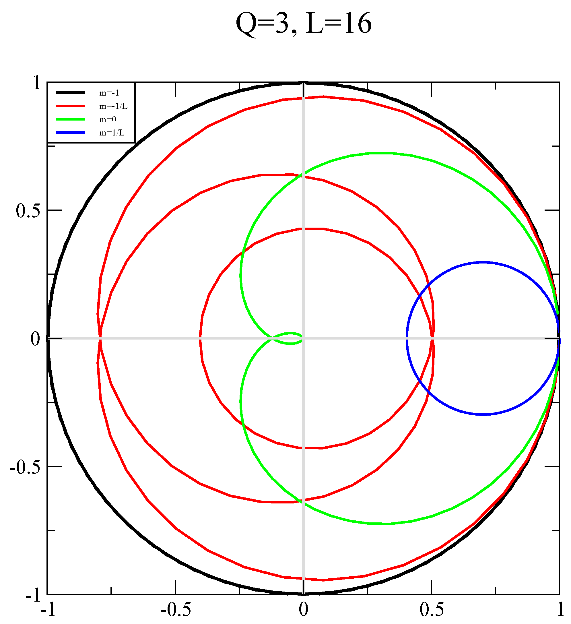
The plot of the full determinant, , is shown for , and in Figure 2, Figure 3 and Figure 4 respectively. In these plots, , and the motion along the closed curve is clockwise starting from the normalized value of . When , the closed curves are unit circles that wind Q times and this is shown for reference in all three plots. We set to be a constant when to maintain a constant physical mass. On the one hand, we see that winds around Q times for and its magnitude changes with . On the other hand, we see that the phase of , reaches a maximum and minimum value in the range for and its magnitude changes with . With the behavior in place for and , we see that is zero and enables a jump in the phase for odd values of Q with it being a smooth function of . Finally, we show the results for in Figure 5. It remains finite as , which is the continuum limit of the background field, and independent of the regulator parameter, .
5. Fermion Determinant in a Non-Abelian Background with Non-Zero
The second background we will consider is a constant background on a torus given by
where are the generators in color space given by Pauli matrices, normalized such that . In this case are all gauge inequivalent and the Chern–Simons action reduces to
Contrary to the Abelian background the phase of the massless fermion determinant is simply given by and we will show this to be the case. Defining as the lattice regulated overlap fermion determinant on a periodic lattice with m being the fermion mass and being another regulator parameter, we will show that both
are both finite and independent of the regulator . This constant SU(2) background can be introduced on the lattice as the link variables
We will consider this background on a three dimensional periodic lattice defined by the points and
All values of that remain finite as are gauge inequivalent.
One can go to momentum space in all three directions and write
where
We have assumed anti-periodic boundary conditions for fermions in the direction. The matrix is given by
where
Let us denote the fermion determinant by on the periodic lattice in this background and define
and
as the determinant with reference to and the determinant at with respect to the free determinant, respectively and is a real function. We will set and and vary . The nonabelian Chern–Simons action given in Equation (58) reduces to and we show the phase of the overlap fermion correctly reproduces this result as in the top panel of Figure 6. Since all are gauge inequivalent, we should find
and we should also find
Both these features are correctly reproduced in the top panel of Figure 6. Since all are gauge inequivalent, we see that the phase at and only approaches as . Note that unlike the Abelian case, the determinant winds around the origin for all values of fermion mass and the fermion determinant remains non-zero for all values of . This is made clear through a plot of in Figure 7.
We note a curious observation in this particular background. The fermion determinant for massless fermions becomes very small for certain values of and it has zeros even at finite L that remains stable as as seen in Figure 7. For our choice of and , we find zeros a pair of zeros at and and another pair at and that remain stable across L. In spite of the fact that all are gauge inequivalent, we see non-trivial behavior seen in the complex determinant for massless fermions in this particular background. Finally, similar to the Abelian background, we found the results for to be finite as and independent of the regulator parameter, .
6. Mixed Chern–Simons (BF) Action and Dualities
Let denote the dependence of the unitary operator in Equation (22) on the Abelian gauge field background, A. A mixed Chern–Simons (BF) term can be written as
One can formally verify the identity by inserting the naïve expressions for CS that are only valid for perturbative fields. The path integrals are defined over all gauge fields and a suitable measure such as a standard Maxwell action for gauge fields is needed to verify the integrals non-perturbatively. Therefore, the last step is essentially a mnemonic and it suggests relations of the form
using a gauge action for A that is implicit and allows one to take a continuum limit (as pointed out explicitly in [3]).
Dualities among various three dimensional theories start with the conjecture [2] that a theory with one massless two component fermion coupled to a dynamical gauge field A and a classical background C defined by
is parity even and dual to a theory at the Wilson–Fisher fixed point. An explicit computation shows that
If , we arrive at a non-trivial relation
where the expectation value is with respect to the measure in Equation (71) and the lattice regularization can be used to verify this relation. In fact, if we use
which has been verified in the continuum limit when a measure for the gauge field is included [18], we see that if we assume that the dynamical fermion has a charge of 2 units,
then is trivially satisfied.
Regularized versions of the various duality relations discussed in [2] can be obtained by following the steps found there. We multiply both sides of Equation (71) by , promote C to the dynamical field with B being a background field and arrive at a regularized version of a fermion-boson duality,
after using Equation (70). If we assume is real we arrive at a regularized version of a boson–boson duality
We can multiply both sides of Equation (71) by , promote C to a dynamical field with B being a background field and arrive at a regularized version of a fermion-fermion duality
and we have used Equations (76) and (77).
A regularized version of a duality involving a fermion with charge of 2 units discussed in [19] can be obtained by setting in Equation (78). In this case, we can multiply both sides by to make the right-hand side even under parity. We also multiply both sides by to couple it to an external flux and promote X to a dynamical field. Then we have
Defining a change of variable, , in the first integral, we obtain
The integral over C can be performed using Equation (70) This forces and we arrive at the regularized version of a fermion-fermion duality
that connects a fermion with 2 units of charge to a fermion with 1 unit of charge.
We should remark that for the sake of simplicity and to a first degree of approximation, we assumed that the massless fermion limits of the odd-flavored theories considered above occurs at the “bare” fermion mass . Unlike the parity-invariant theories with SU flavor symmetry with being even, where the mass term is protected by the symmetry, there is no such symmetry consideration in odd flavored theories. Thus, it could be possible that one needs to tune the overlap fermion mass in order to reach criticality, provided there is one. In that case, the above set of equations might have to be modified accordingly with such mass terms, but it is a straightforward exercise.
7. Conclusions
Overlap formalism was developed three decades ago [7] to properly reproduce all salient features of massless fermions in even dimensions. This was extended to odd dimensions in [10] and we showcase the salient features of massless fermions in odd dimensions; particularly, we extended the formalism and spell out the lattice constructions of topological gauge actions that are being investigated currently in the context of TQFTs coupled to fermions, and in the context of infrared dualities. We focused on the overlap fermion determinant and used two examples, one Abelian background and one non-Abelian background. We showed that the overlap fermion determinant correctly reproduces all known properties of the phase of the fermion determinant; especially, we discussed how the lattice regularization manages to implement the half-Chern–Simons term (or half-the-eta-invariant) in a gauge-invariant manner. While it is satisfying that we can nonperturbatively formulate the topological gauge theories on the lattice, an actual numerical study of such theories is not yet practical due to the sign problem and we did not address such issues in this paper.
An interesting possibility of having a lattice regularized Chern–Simons theory is the following. As we noted in this paper, it is important to realize that the identification of overlap with the continuum Chern–Simons action is possible only in the continuum limit (as usual, the continuum limit taken at the trivial UV fixed point of the lattice gauge theory). However, as a lattice gauge theory that is away from any critical points, the overlap fermion determinants offer a great way to introduce new parity-odd gauge-invariant gauge-actions. Thus, one could now ask about the phase diagrams of such well defined lattice gauge theories as a function of different lattice couplings. This is an exciting direction to think about in the future.
Author Contributions
Conceptualization, N.K. and R.N.; methodology, N.K. and R.N.; software, N.K. and R.N.; investigation, N.K. and R.N.; writing—original draft preparation, R.N.; writing—review and editing, N.K.; visualization, N.K. and R.N.; funding acquisition, N.K. and R.N. All authors have read and agreed to the published version of the manuscript.
Funding
R.N. acknowledges partial support by the NSF under grant number PHY-1913010. N.K. is supported by Jefferson Science Associates, LLC under U.S. DOE Contract #DE-AC05-06OR23177 and in part by U.S. DOE grant #DE-FG02-04ER41302.
Data Availability Statement
Data available up on request.
Conflicts of Interest
The authors declare no conflict of interest.
References
- Dunne, G.V. Aspects of Chern–Simons theory. In Aspects Topologiques de la Physique en Basse Dimension. Topological Aspects of Low Dimensional Systems; Springer: Berlin/Heidelberg, Germany, 1999. [Google Scholar]
- Seiberg, N.; Senthil, T.; Wang, C.; Witten, E. A Duality Web in 2+1 Dimensions and Condensed Matter Physics. Ann. Phys. 2016, 374, 395–433. [Google Scholar] [CrossRef] [Green Version]
- Karch, A.; Tong, D. Particle-Vortex Duality from 3d Bosonization. Phys. Rev. 2016, X6, 031043. [Google Scholar] [CrossRef] [Green Version]
- Wang, C.; Nahum, A.; Metlitski, M.A.; Xu, C.; Senthil, T. Deconfined quantum critical points: Symmetries and dualities. Phys. Rev. 2017, X7, 031051. [Google Scholar] [CrossRef] [Green Version]
- Bilal, A. Lectures on Anomalies. arXiv 2008, arXiv:0802.0634. [Google Scholar]
- Atiyah, M.F.; Singer, I.M. The index of elliptic operators on compact manifolds. Bull. Am. Math. Soc. 1969, 69, 422–433. [Google Scholar] [CrossRef] [Green Version]
- Narayanan, R.; Neuberger, H. A Construction of lattice chiral gauge theories. Nucl. Phys. 1995, B443, 305–385. [Google Scholar] [CrossRef] [Green Version]
- Neuberger, H. Geometrical aspects of chiral anomalies in the overlap. Phys. Rev. 1999, D59, 085006. [Google Scholar] [CrossRef] [Green Version]
- Coste, A.; Luscher, M. Parity Anomaly and Fermion Boson Transmutation in Three-dimensional Lattice QED. Nucl. Phys. 1989, B323, 631. [Google Scholar] [CrossRef]
- Kikukawa, Y.; Neuberger, H. Overlap in odd dimensions. Nucl. Phys. 1998, B513, 735–757. [Google Scholar] [CrossRef] [Green Version]
- Narayanan, R.; Nishimura, J. Parity invariant lattice regularization of three-dimensional gauge fermion system. Nucl. Phys. 1997, B508, 371–387. [Google Scholar] [CrossRef]
- Bietenholz, W.; Nishimura, J. Ginsparg-Wilson fermions in odd dimensions. JHEP 2001, 7, 015. [Google Scholar] [CrossRef] [Green Version]
- Bietenholz, W.; Nishimura, J.; Sodano, P. Chern–Simons theory on the lattice. Nucl. Phys. B Proc. Suppl. 2003, 119, 935–937. [Google Scholar] [CrossRef] [Green Version]
- Karthik, N.; Narayanan, R. Phase of the fermion determinant in QED3 using a gauge invariant lattice regularization. Phys. Rev. 2015, D92, 025003. [Google Scholar]
- Alvarez-Gaume, L.; Della Pietra, S.; Moore, G.W. Anomalies and Odd Dimensions. Ann. Phys. 1985, 163, 288. [Google Scholar] [CrossRef]
- Witten, E. Three lectures on topological phases of matter. Riv. Nuovo Cim. 2016, 39, 313–370. [Google Scholar]
- Karthik, N.; Narayanan, R. Scale-invariance of parity-invariant three-dimensional QED. Phys. Rev. 2016, D94, 065026. [Google Scholar] [CrossRef] [Green Version]
- Karthik, N.; Narayanan, R. Parity Anomaly Cancellation in Three-Dimensional QED with a Single Massless Dirac Fermion. Phys. Rev. Lett. 2018, 121, 041602. [Google Scholar] [CrossRef] [PubMed] [Green Version]
- Cordova, C.; Hsin, P.S.; Seiberg, N. Time-Reversal Symmetry, Anomalies, and Dualities in (2 + 1)d. SciPost Phys. 2018, 5, 6. [Google Scholar] [CrossRef]
Figure 1.
The top panel shows the flow of the phase in the infinite mass case, , as a function of Wilson-loop variable at . The Wilson mass entering the kernel of overlap operator is fixed at . For fixed , the variation with reduction in lattice spacing by increasing L from 4 to 8 is also shown. The bottom panel shows similar flow of the phase of the determinant in the massless case. The variability with respect to the regulator parameter and lattice spacing are shown.

Figure 2.
The flow of the overlap fermion determinant in the complex plane as a function of at a fixed on lattice. The flows are shown for 1 (black), (red), 0 (green), (blue). The flow starts at for , goes clockwise and returns back to for .
Figure 2.
The flow of the overlap fermion determinant in the complex plane as a function of at a fixed on lattice. The flows are shown for 1 (black), (red), 0 (green), (blue). The flow starts at for , goes clockwise and returns back to for .

Figure 3.
The flow of the overlap fermion determinant in the complex plane as a function of at a fixed on lattice. The description is the same as in Figure 2.
Figure 3.
The flow of the overlap fermion determinant in the complex plane as a function of at a fixed on lattice. The description is the same as in Figure 2.

Figure 4.
The flow of the overlap fermion determinant in the complex plane as a function of at a fixed on lattice. The description is the same as in Figure 2.
Figure 4.
The flow of the overlap fermion determinant in the complex plane as a function of at a fixed on lattice. The description is the same as in Figure 2.

Figure 5.
The plot demonstrates the existence of the continuum limit of the overlap fermion action in constant flux background at zero . The continuum extrapolations () are shown using an expansion in lattice spacing . The consistency in the extrapolated values using different regulator parameter is seen.

Figure 6.
The figure is similar to Figure 1 showing the flow of the phase of the fermion determinant as a function of SU(2) gauge field magnitude . The top panel shows the result for infinitely massive fermion, with regulator parameter . The convergence of the results at different L towards a continuum result is shown. The bottom panel shows the flow with at different fermion masses m.

Figure 7.
The dependence of the magnitude of the fermion determinant on . The result at zero and non-zero masses are shown. The determinant at zero mass vanishes are certain values of , though not for any reasoning from invariance under large gauge transformation as seen in the case of Abelian background field studied in this paper.

Publisher’s Note: MDPI stays neutral with regard to jurisdictional claims in published maps and institutional affiliations. |
© 2022 by the authors. Licensee MDPI, Basel, Switzerland. This article is an open access article distributed under the terms and conditions of the Creative Commons Attribution (CC BY) license (https://creativecommons.org/licenses/by/4.0/).
Share and Cite
MDPI and ACS Style
Karthik, N.; Narayanan, R. Topological Gauge Actions on the Lattice as Overlap Fermion Determinants. Universe 2022, 8, 332. https://0-doi-org.brum.beds.ac.uk/10.3390/universe8060332
AMA Style
Karthik N, Narayanan R. Topological Gauge Actions on the Lattice as Overlap Fermion Determinants. Universe. 2022; 8(6):332. https://0-doi-org.brum.beds.ac.uk/10.3390/universe8060332
Chicago/Turabian StyleKarthik, Nikhil, and Rajamani Narayanan. 2022. "Topological Gauge Actions on the Lattice as Overlap Fermion Determinants" Universe 8, no. 6: 332. https://0-doi-org.brum.beds.ac.uk/10.3390/universe8060332
Note that from the first issue of 2016, this journal uses article numbers instead of page numbers. See further details here.