
Chemical Tracing and the Origin of Carbon in the Galactic Disk

1
Department of Physics and Astronomy, Uppsala University, 751 20 Uppsala, Sweden
2
Nordic Institute for Theoretical Physics (Nordita), 106 91 Stockholm, Sweden
Universe 2022, 8(8), 409; https://0-doi-org.brum.beds.ac.uk/10.3390/universe8080409
Submission received: 13 January 2022
/
Revised: 14 July 2022
/
Accepted: 30 July 2022
/
Published: 4 August 2022
(This article belongs to the Special Issue AGB Stars—In Honor of Professor Maurizio Busso on the Occasion of His 70th Birthday)
Abstract
:A basic problem in studies of the evolution of chemical elements in galaxies is the uncertainties in the yields of elements produced by different types of stars. The possibilities of tracing the sites producing chemical elements and corresponding yields in stellar populations by studying ratios of abundances in stars of different ages and metallicities, with an approach with minimal assumptions concerning the yields, is explored by means of simple models of Galactic chemical evolution. Elemental abundances of carbon and oxygen, obtained by recent observations of samples of solar-type stars with estimated ages in the thin disk of the Galaxy, are analysed. Constraints on the yields from winds of intermediate-mass stars and of hot massive stars, including core-collapse supernovae, are derived. It is found that a dominating contribution of carbon from massive stars is most probable, although stars in the mass interval of two to three solar masses may have provided some amounts of carbon in the Sun. The results are consistent with those obtained by using theoretical yields and more elaborate models of Galactic evolution. The uncertainties as regards the mixing of stellar populations due to migration of stars in the Galactic disk may be important for the conclusions. Variations in the star formation rates, lack of chemical homogeneity in the Galactic gas, the inflow of gas from the intergalactic space and possible variations in the Initial mass function may also limit conclusions about the sites and their yields. Very accurate abundance ratios and the determination of stellar ages provide further important constraints on the yields.
1. Introduction
Sixty years ago Wallerstein [1] observed that the ratio of the stellar abundances of elements such as magnesium and titanium—which originate in massive stars—relative to that of iron, are higher for high velocity Halo stars than for stars residing in the Galactic disk. Iron is now known to a great extent come from less massive stars. This finding was interpreted by Tinsley [2] as a natural consequence of the smaller initial stellar mass, and thus longer life-times, of stars in iron-producing SNe Ia, compared with those of SNe II which are mainly responsible for the production of oxygen and the elements.
Since then, it has become customary to plot the logarithmic chemical abundance ratios, such as [Mg/Fe] relative to [Fe/H] for individual stellar atmospheres (the square brackets then indicating that the ratios have been normalised to the corresponding quantities for the Sun), see e.g., [3,4,5]. The slopes and other tendencies in these diagrams contain information about the origin and the history of the nucleosynthesis of the elements involved. During the last decades the abundance data have grown and improved considerably in quantity and quality through very impressive spectroscopic surveys, such as the Gaia-ESO [6], the APOGEE [7], the GALAH [8], and the LAMOST [9] surveys. Moreover, the analyses of the spectroscopic data have also been improved by physically sound modelling of convection and radiative transfer in the stellar atmospheres and of the effects of departures from Local Thermodynamic Equilibrium on the stellar spectra ([10] and papers cited therein [5,11]), and by limiting the parameters of the sample of stars to enable strictly differential analyses [12,13].
Analyses of these types of data are frequently made by using models of the evolution of the chemical elements in the Galaxy and other galaxies. Such models were pioneered by Schmidt [14], Salpeter [15], Truran and Cameron [16], Lynden-Bell [17], Pagel and Patchett [18] and Tinsley [19] and the numerous newer and extended models were recently summarised by Matteucci [20]. These models are constructed on the basis of a number of theories and assumptions concerning star formation, Galactic dynamics, gas accretion to the Galaxy and winds from it, and not the least concerning nucleosynthesis in stars and stellar mass loss from lower-mass and intermediate-mass stars (LIMS) in their AGB and post-AGB phases, including their evolution in binaries sometimes leading to mass transfer and thermonuclear explosions such as Supernovae Type Ia, or contributions of chemical elements from high mass stars (HMS) in their evolution with hot radiatively driven winds, as Wolf–Rayet stars or finally core-collapse Supernovae Type II. A number of uncertainties are obviously built into these models, and in practice handled by free parameters, more or less constrained by various considerations, and often in the end set by fitting the observations of chemical abundances as found from stellar spectra.
The present paper attempts to trace the effective yields from different types of stars, and in particular to decide whether LIMS or HMS are dominating for a particular element, by studying the abundance ratios observed for solar-type stars of different ages in the Galactic disk. The spectra of these stars are thought to rather well reproduce the chemical composition of the interstellar gas in which they were formed. Additionally, their atmospheric structures are relatively well understood so that their spectra may be well analysed and accurate differential measurements relative to the Sun are possible. A semi-empirical approach with a minimal use of theoretical yields of chemical elements from stellar models is presented. It could serve as a test of such theoretical yields. The method will be applied in an attempt to resolve the problem of the origin of the carbon in the Solar system.
The candidate sites for producing carbon in the Galaxy are primarily massive stars, including core-collapse supernovae and Wolf–Rayet stars [21] and references therein, and LIMS on the Asymptotic Giant Branch (AGB) and thereafter ([22,23]). The relative significance of these sites has been repeatedly discussed. For a summary of the early discussion, see [24], where we concluded from measurements of the [C I] 8727 Å line in spectra of solar-type stars that massive stars were the most probable contributors of carbon in the Galaxy. This was based on the observed slope in the [C/Fe]-[Fe/H] diagram for Galactic stars and also data for H II regions in metal-poor galaxies. Henry et al. [25] also found support for this origin of carbon from Galactic and extra-galactic HII regions while Chiappini et al. ([26,27]), as well as well as Bensby and Feltzing [28] and Mattsson [29] found evidence for carbon production by LIMS. In their review Karakas and Lattanzio [23] drew the conclusion that about equal amounts of solar carbon originated in core-collapse SNe and in AGB stars, respectively. More recent studies, based on improved and much more extensive data for stars and nebulae in the Milky Way and other galaxies, suggest that most of the Galactic carbon came from massive stars (Griffith et al. [30], Franchini et al. [31], see also the review by Randich and Magrini [32]).
2. The Model Equations
2.1. The Galactic Disk
A simple one-zone model is used here to represent the evolution of a stellar population in a galaxy, with several features in common with models used frequently in contemporary studies, for a summary see Matteucci [20] whom we follow here, although in the present paper a parametrised description is used for the yields of LIMS and empirical data on abundances and ages are used more directly. We may write, for the mass fraction of element e in the gas with projected surface density onto the galactic plane:
Here, the first term on the RHS represents the loss of nuclei from the interstellar medium by star formation (“astration”) while the second term represents the addition of nuclei to the medium by stellar mass loss. The integrals are taken between and . A time-constant IMF, the distribution of stellar initial mass m, is adopted:
The star-formation rate is assumed to scale with the surface gas density:
where is “the star formation efficiency”, and is a constant. is set to zero for , the time from the formation of a star with mass m and initial metallicity Z, until it delivers its major contribution of processed material to the interstellar medium. The net in-falling gas is assumed to be metal-poor, while the in-falling metal-rich gas is assumed to be compensated for by the corresponding outgoing flow, , so that both these two latter flows cancel.
The values of are set to 2.3 for and for following Kroupa [33], and the value of is set to 1.4, following Kennicutt and Evans [34]; the consequences of varying these values are explored.
A logarithmic time-metallicity relation for the initial composition of the stars is adopted,
where t is in Gyr. Other recipes were also tried, e.g., a saw-toothed pattern to mimic the possible variation in metallicity (or at least iron abundance) traced by Nissen et al. [13]. This had only minor consequences for the result. and are usually set to 0.009 and 0.018 for the time t in Gyr, However, a clear age–metallicity relation is known not to exist in the Galactic disk, why other alternatives were also tried, e.g., with relations chosen to fit the time–metallicity relation of Thin Galactic disk stars or for the younger stars (blue symbols in Figure 3 of Nissen et al. [13]).
For elements almost exclusively produced by HMS, such as oxygen and magnesium with as compared with the life time of the LIMS, one may write Equation (1):
Here, is set to 11 . If the time variation of the abundance is observed and set into Equation (5), it may be used to estimate the surface density of the gas, .
2.2. The LIMS Yields
The yield of any element e from low- and intermediate-mass stars is parametrised in the following way: a parabolic mass dependence is assumed with a maximum at mass and a half width of . The parabola is:
For , i.e., , the profile is usually set to zero. However, alternatively an additional contribution, extending to masses up to is allowed. Thus a correction may be added to the yield so that:
with
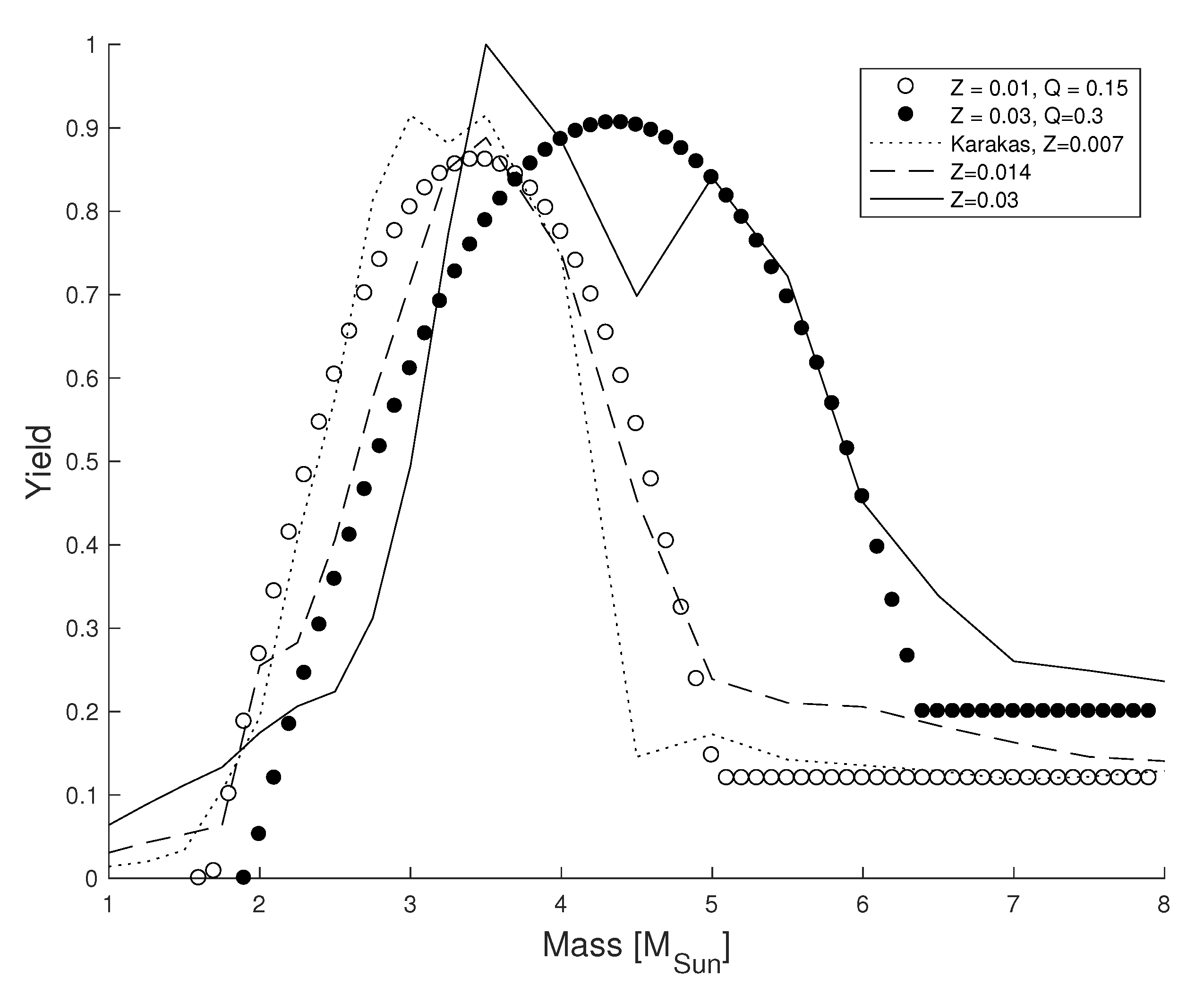
The constant Q is typically given values from 0.0 to 0.6 . Some resulting yield profiles as functions of stellar mass are illustrated in Figure 1. In the figure, also theoretical carbon yields for AGB stars according to Karakas and Lugaro [35] have been plotted.
A possible variation of the yields with stellar metallicity must also be accounted for. This effect has been parametrised by adopting linear variations of and ,
and
Typical values chosen for and are 0 and 1 .
2.3. The HMS Yields
The yields for elements produced by HMS have been adopted from Limongi and Chieffi [37], with a weighting of 0.75 for non-rotating models and 0.25 for models with rotation speeds of 150 km/s. Since the model of Equation (1) will not be applied to the early evolution of galaxies one may work at a lower time resolution and treat the contributions to the abundance through winds from short-lived massive stars in a much simpler way than by detailed integration. The yields for element e, integrated for all HMS, may thus be parameterised by one single function of metallicity, , but the values of this integrated yield are quite uncertain, due to the lack of knowledge concerning the effects of rotation and duplicity on the evolution and mass loss from massive stars, and concerning the precise mass cut in the core-collapse supernovae. These uncertainties are tentatively accounted for by adding corrections to the HMS yields by Limongi and Chieffi [37], setting:
where denotes Limongi et al. yields. The constant g is allowed to vary from 0 to 20 to monitor the effect of varying the contribution of HMS with respect to LIMS, in particular to study the effects on the relative contributions to the carbon abundance in the Sun (see below). is chosen with values 0 and 1 . The latter value obviously corresponds to a doubling of the contribution of the element from massive stars when the metallicity increases through the evolution of the Disk.
2.4. Initial Conditions
In order to solve Equations (1) and (5) we need to specify initial conditions. The integration of the first equation proceeds from a starting time of the disk evolution, chosen to be 9 Gyr ago. The initial oxygen abundance is set to a factor of the solar abundance, and for carbon produced by HMS similarly times the solar carbon produced by HMS. Typically the f values were set to 0.5. Equation (5) was integrated backwards in time, with the present gas surface density of 13.7 , following McKee et al. [38], as an initial value.
An overview of the different parameters in our model simulations is presented in Table 1.
3. Diagnostics and Observations
3.1. The Time Variation of [O/H] and the Gas Density
A reference element for estimating the evolution of the gas density in the Galactic disk by Equation (5)), is oxygen, which is mainly provided by massive stars. O nuclei may also be produced in intermediate-mass stars by helium burning, but much of this oxygen is converted into nitrogen or heavier elements, so that the net yields of the element by these stars are minute (e.g., Karakas and Lugaro [35], Karakas et al. [36]). Here oxygen abundances for stars of different ages are adopted from Nissen et al. [13], who used spectra of very high quality () for 72 solar-like stars to measure the oxygen abundance from the [O I] 6300.3 Å line. The stellar ages, adopted from the same source, were based on model isochrones, effective temperatures and heavy element abundances from the spectra, and luminosities from Gaia parallaxes. The errors in the ages were estimated to be 1 Gyr or less.
As an alternative, the study of 78 solar-like stars by Bedell et al. [39] was used. Here, the spectra were of very high quality, while the oxygen abundances were derived from the 7771–7774 Å triplet lines with corrections for departures from LTE. The ages were again based on (a different set of) isochrones, and an earlier Gaia release.
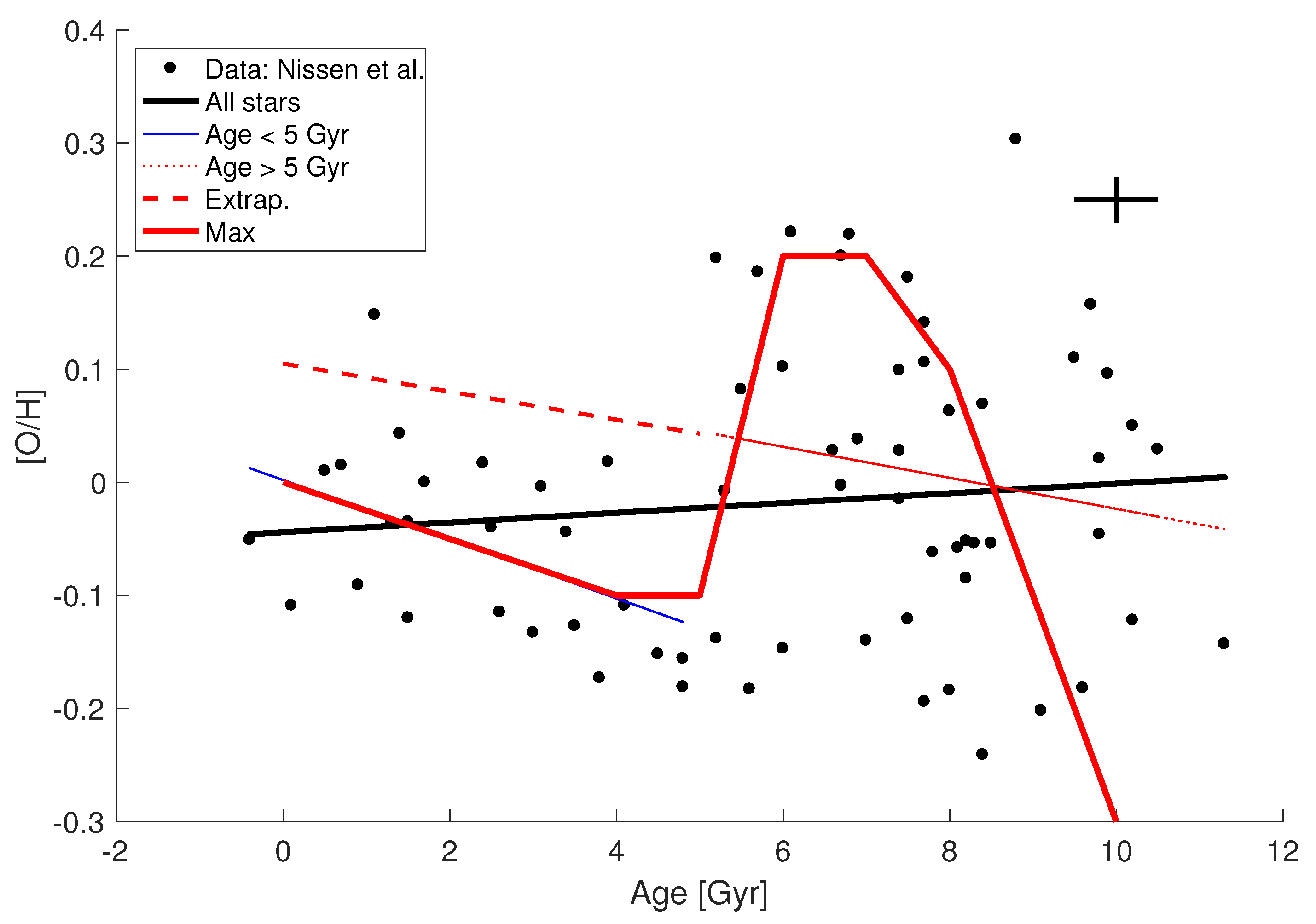
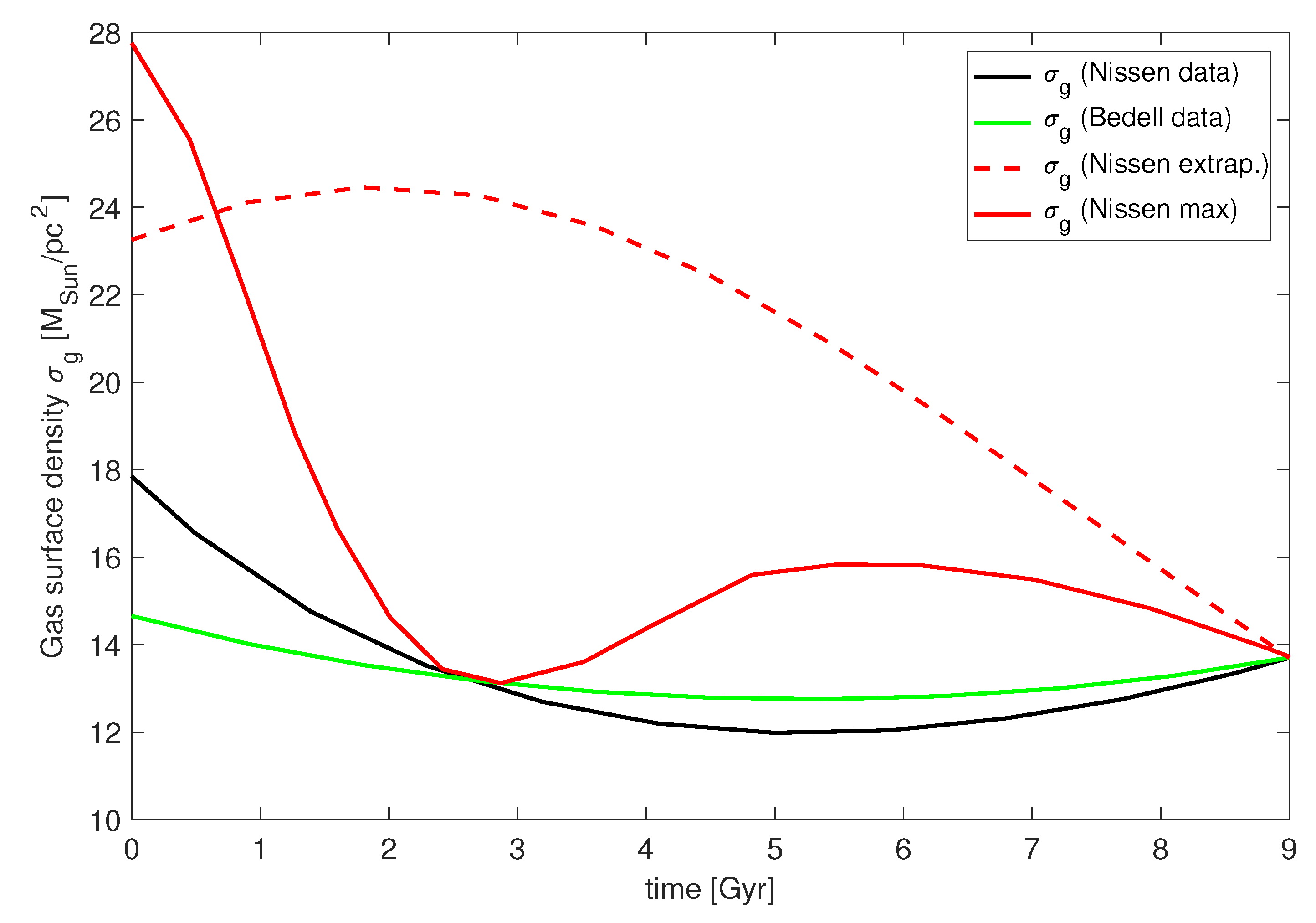
The resulting oxygen abundances relative to stellar age are shown in Figure 2. Here also several lines are plotted, showing regressions (with estimated observational errors in both directions considered), for all the stars, and for stars younger and older than 5 Gyr separately. This latter division takes into account the finding by Nissen et al. that separate abundance patterns appear for the disk stars at about this age. In the diagram also some schematic different relations are shown, where the tendency for older stars are extrapolated towards younger ages (red dashed), or where mean oxygen abundance is assumed to vary more drastically with time (thick red line, denoted in the figure by “Max”, and referred to “Nissen max”, below). These different relations were next used as input into Equation (5). The resulting variations of the density with time are shown in Figure 3, which also shows the density variation that results if the oxygen abundances and ages by Bedell et al. [39] are adopted. As is suggested by Figure 3, the surface density may have stayed fairly constant during the history of the (thin) Disk, meaning that the amount of infalling pristine gas seems to have been compensated for by star formation.
Since the observed oxygen abundance is also rather constant during the history of the disk, it is of interest to explore the implications when the time derivatives in Equation (5) or in Equation (1) are small, that is when , which in particular happens when the disk is aging. Obviously, this means that the two first terms in the RHS of Equation (1), the “astration term” and the “production term” tend to balance—the oxygen mass stored in new stars by star formation and the amount of oxygen produced and emitted from the stars are roughly equal. From Equation (5) follows then
Obviously, the abundance is determined by the ratio between the IMF, , as weighted by the yield , relative to the IMF weighted by the stellar mass. Adopting the yields from Limongi and Chieffi [37] one then finds from Equation (12) for the oxygen abundance by weight , which is in perfect agreement with the observed solar value according to Asplund et al. [40] of 0.0057. Even more interesting is that the abundance of carbon, if only produced by HMS, is found from the theoretical yields and Equation (12) to be 0.0023, close to the observed Solar value of 0.0025. It should be noted that the weighted MS yields, according to Limongi and Chieffi [37] are not very dependent on metallicity. Therefore, with the provision that the systematic time dependence of and of the O abundances in the disk gas are relatively small, this finding suggests that the abundances of both oxygen and carbon may be understood as the result of HMS stars. This possibility will be discussed subsequently on the basis of additional data.
3.2. The Abundance–Abundance Diagram
The focus will now be on the diagram where the logarithmic abundance by the number of nuclei of element e is plotted relative to the abundance of reference element r, the latter essentially produced by massive stars. It should be noted that this diagram departs from the convention in most studies (including Gustafsson et al. [24]) where the reference element has been iron, which in the Galactic disk to a considerable extent is produced by relatively long-lived stars via Supernovae Type Ia. Although having advantages spectroscopically, the choice of iron tends to make the interpretation of the diagram more complicated. The logarithm of the abundance ratio will be normalised to the solar value and denoted by and then plotted relative to the logarithmic abundance of r relative to hydrogen, [r/H], again normalised relative to the solar abundance ratio. The abundance ratios as functions of time will be modeled by solving Equations (1) and (5). The simulation of the Galactic disk is started at a time 9 Gyr before the present time, and is set to 4.3 Gyr when the solar abundances will be read off and then used for normalizing the logarithmic abundance ratios. (We here neglect the tendencies for atypical solar abundance ratios found by Meléndez et al. [12]).
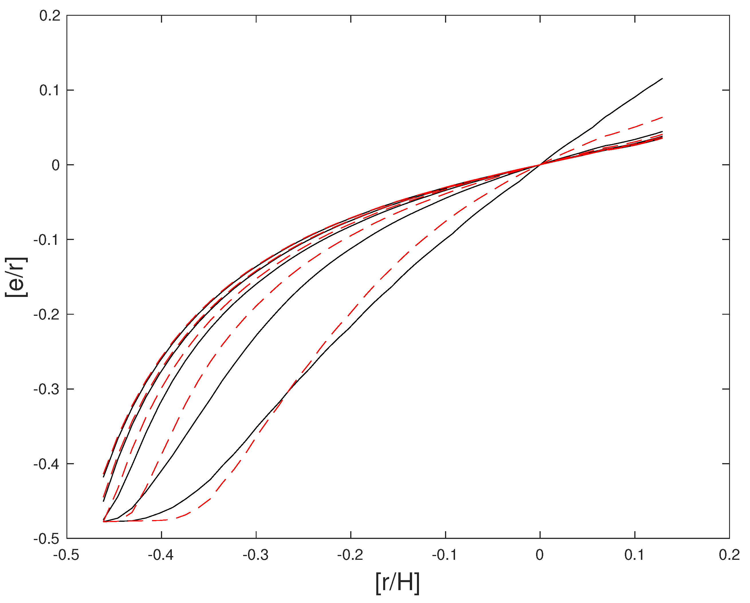
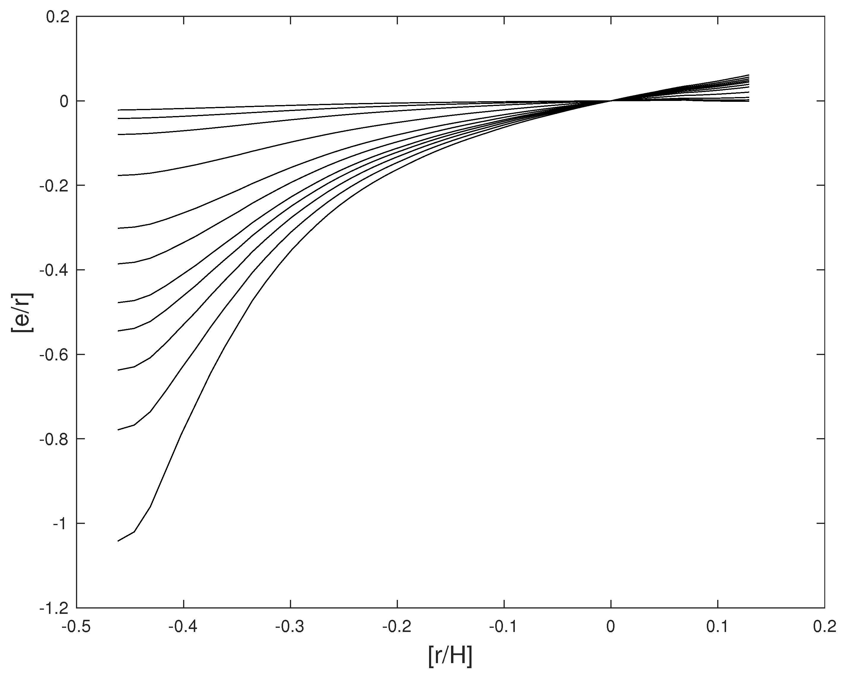
Some typical results plotted for different choices of model parameters are displayed in Figure 4 and Figure 5. All these curves reflect the increasing contribution of the element e by LIMS as they reach the AGB stage, and the abundance of the reference element increases with time, as measured by [r/H]. The higher the initial mass of the LIMS, the earlier they contribute. We also see in Figure 4 that narrowing the yield peak in mass makes the slopes of the curves smaller at late times since the steep IMF then admits much fewer stars from the numerous low-mass stars to contribute. A related effect is found when the yield function is widened to higher masses by setting . The effects are relatively small and again decrease the slope in the diagram. What matters for the slope is the normalised yield weighted by the IMF, and then the low-mass end of the yield function is most significant.
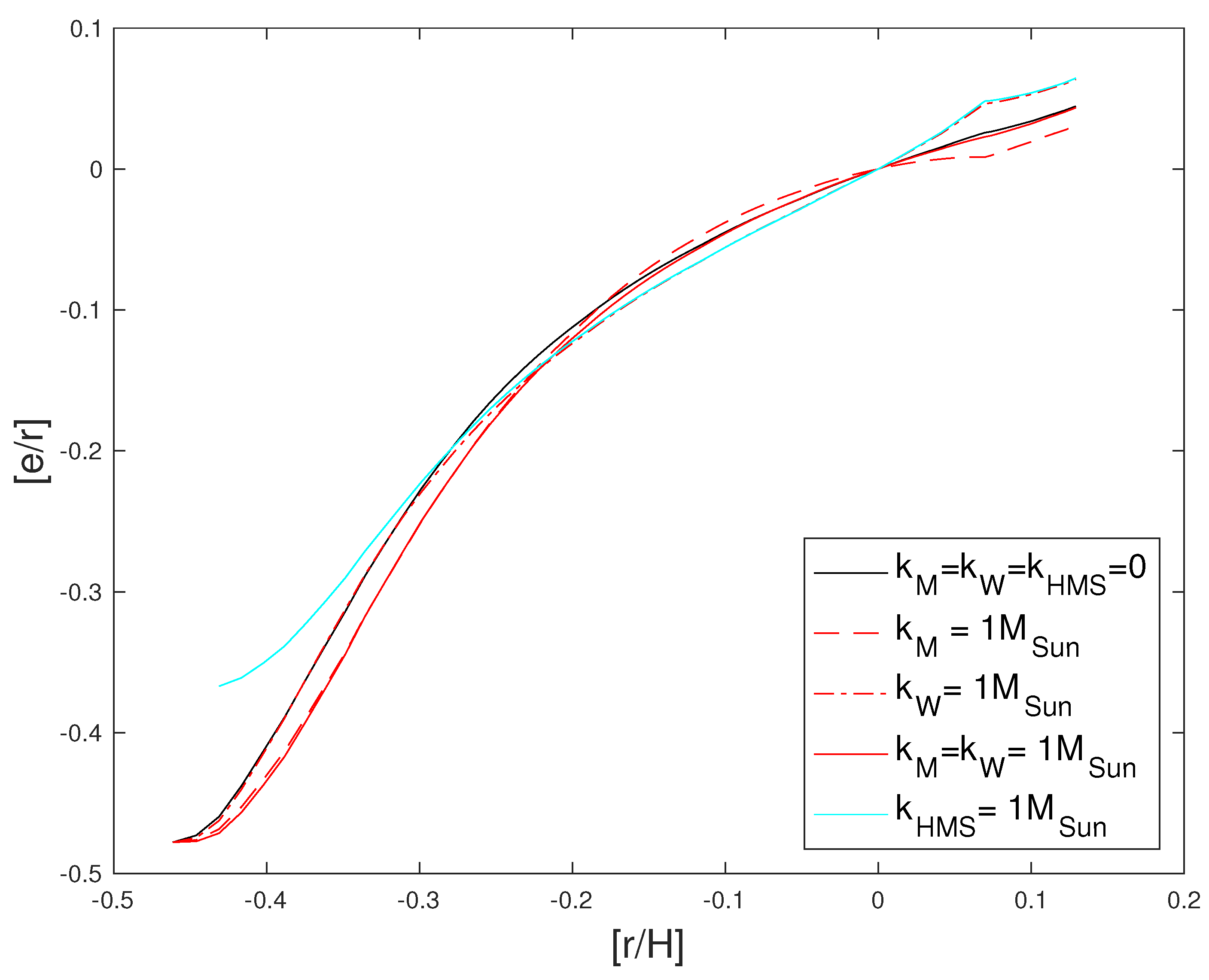
The effects from metallicity changes of the yields are shown in Figure 5. As is seen, these effects are rather small, which to a great extent is due to the compensation by the normalization of the abundances on the solar values.
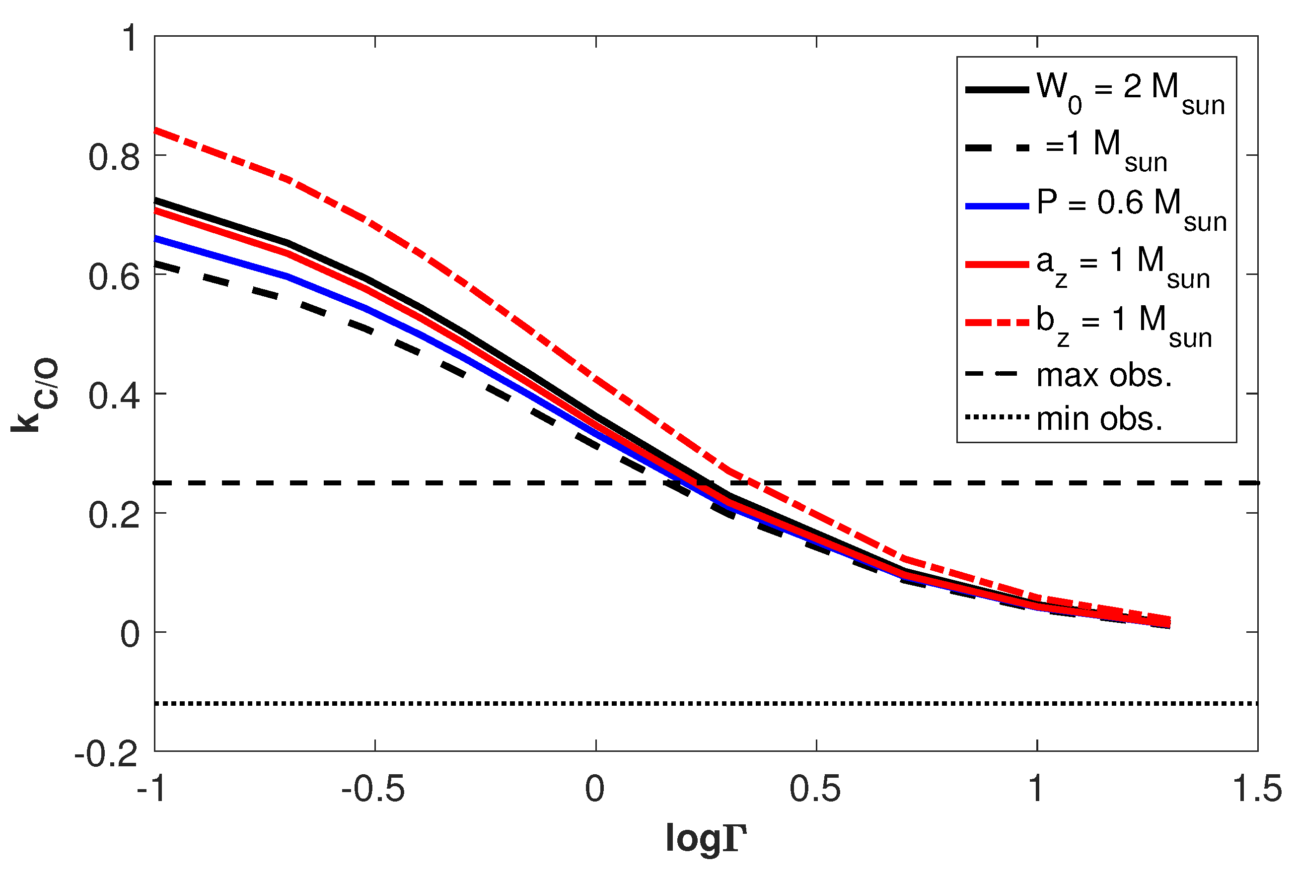
A main objective of the present study is to explore whether the origin of elements can be conclusively traced to either massive stars or intermediate-mass stars. Therefore, the result of varying the parameter g, regulating the contribution of element e from stars of different masses is of particular interest. This is explored in Figure 6 where the curves in the diagram show results for different fractions of the element e produced by massive stars, as compared with LIMS.
Aiming at tracing the yields of stars contributing to the observed elemental abundances, one also has to consider the effects that uncertainties in Galactic evolution may introduce. This has been schematically explored by varying the parameters of the simple Galactic model. Some outcomes are illustrated in Figure 7. Changes in the surface density of gas, as estimated from the observed variation of [O/H] with time from Equation (5), may, as seen in Figure 7, lead to considerable changes in the [e/r]-[r/H] curves. If instead the star-formation rate R is assumed to vary exponentially with time as with we find that a change of the characteristic time T from 5 Gyr to 2 Gyr will change the slope of the curve by about 10%. A more rapid star formation deceases the slope, which reflects the swifter building up of the reference element r by massive stars while the production by LIMS comes later. The effects of changing the typical decay time of gas infall into the disk from 5 to 20 Gyr are of similar size. The effects of changes of the IMF are minor.
In order to use these theoretical results to constrain yields we define a characteristic indicator, the slope k in the abundance–abundance diagram, i.e.,
where the points 1 and 2 along the curves are usually selected at [r/H] vales of −0.30 and 0.20, respectively. In Figure 8 and Figure 9, this quantity is plotted relative to , for different parameter sets.
The possibility to also use the second derivative, the curvature, of the relation in the abundance–abundance diagram to constrain the parameters is challenging, since very high accuracy is needed in the abundance measurements in order to enable meaningful results. Moreover, a real cosmic scatter in abundances, due to mixing of different stellar populations or other reasons for individual abundance characteristics for different stars, may limit the possibilities. Experiments have indicated that this additional measure may primarily be useful for constraining the peak mass of LIMS profiles with < 3 M. Another possibility is, however, to use the curvature measure to verify effects of strongly varying surface gas densities, disclosing effects such that shown by the “Nissen max” curve in Figure 7.
3.3. The Abundance-Ratio versus Time Relation
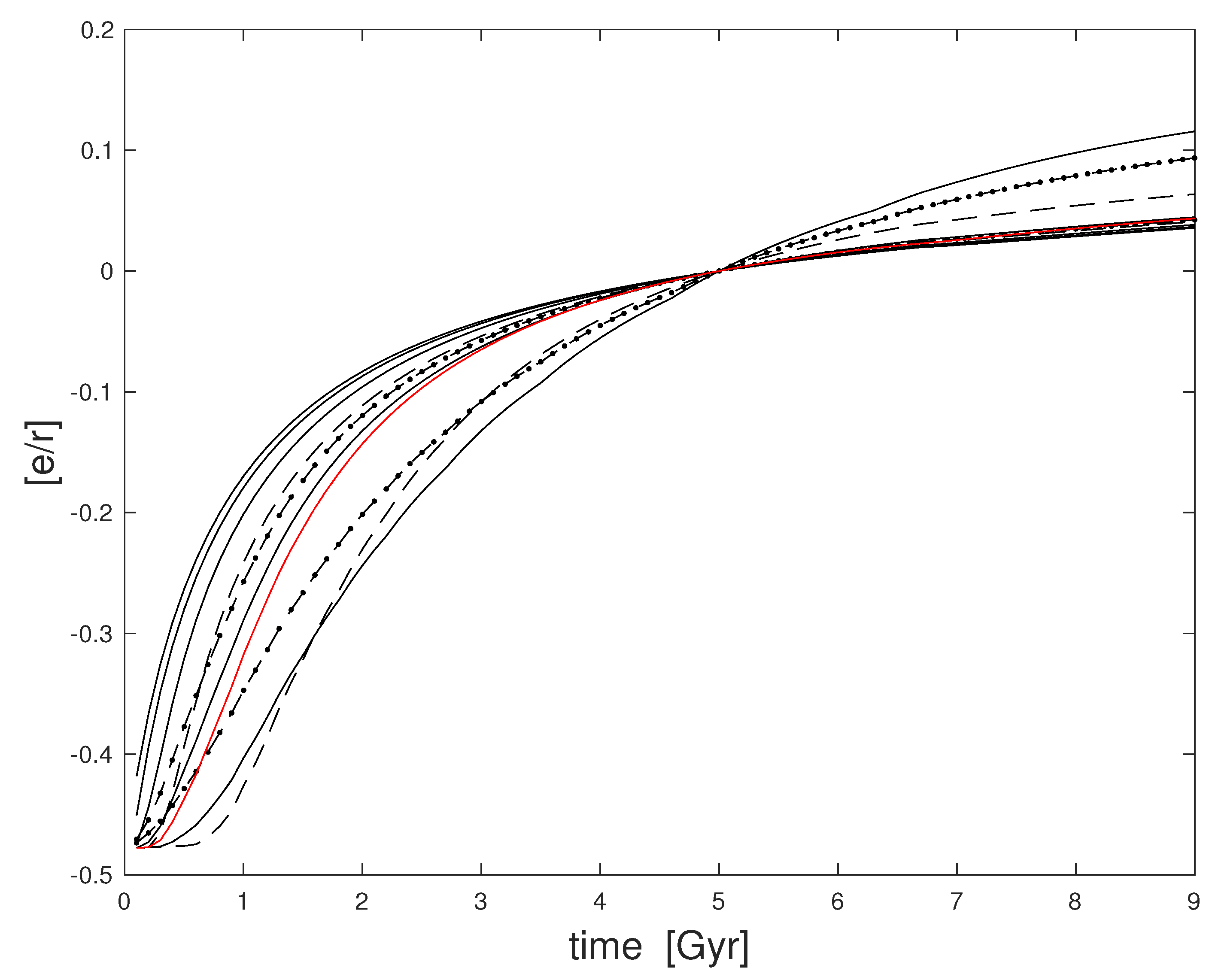
Recent impressive advances in dating stars have opened up yet another possibility to constrain the yields of elements. Thus, the Gaia parallaxes have made the use of isochrones more accurate (e.g., Sahlholdt et al. [41], Nissen et al. [13]), and the astereoseismic data, constraining the stellar mean mass densities, admit in combination with other stellar data age determinations also for distant giant stars [42,43]. Examples of relations between [e/r] and time, calculated by the present simple model are shown in Figure 10 for different parameter sets. One may use the slope in this diagram as a characteristic of the chemical evolution in a galaxy. A quantity has been introduced:
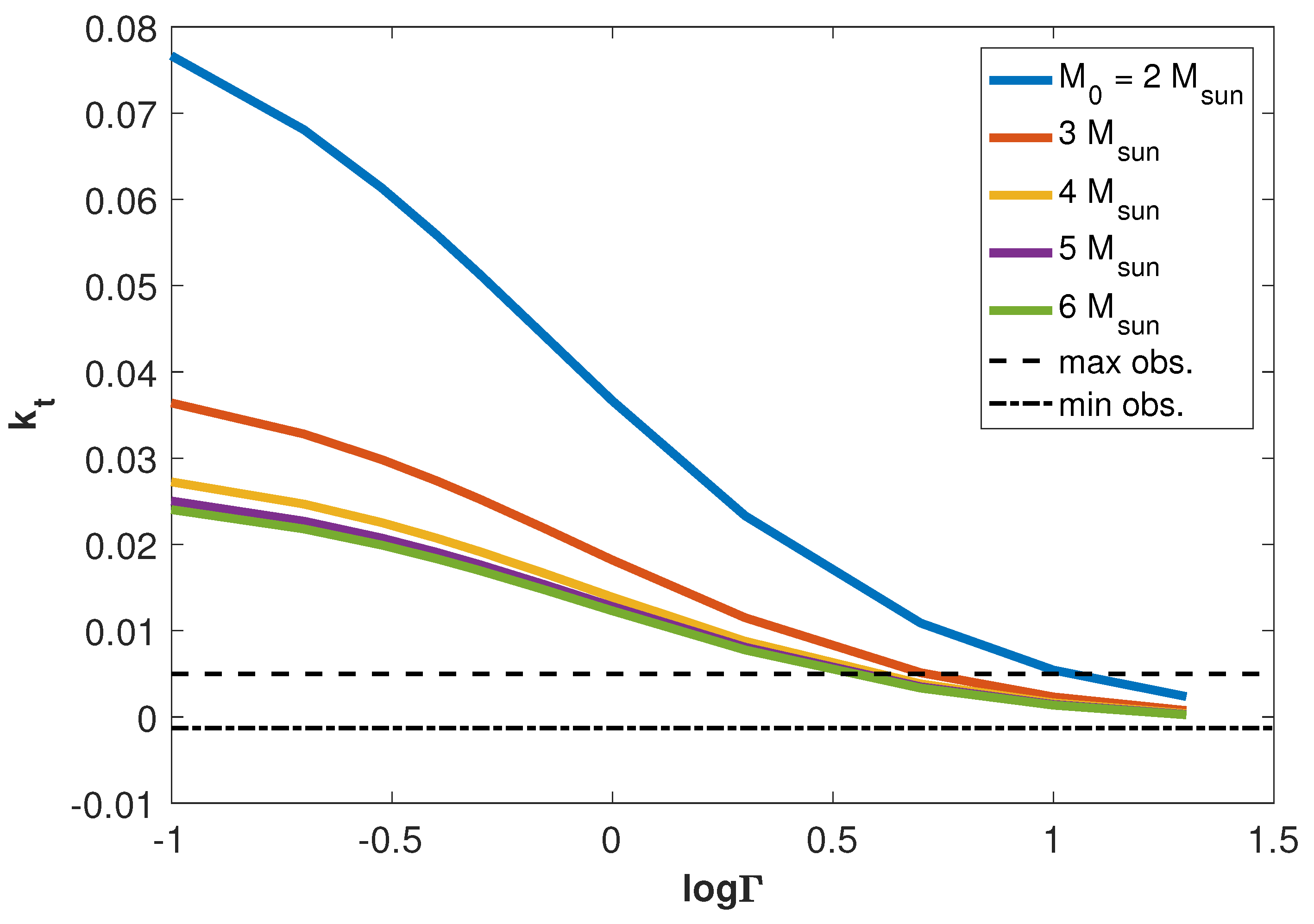
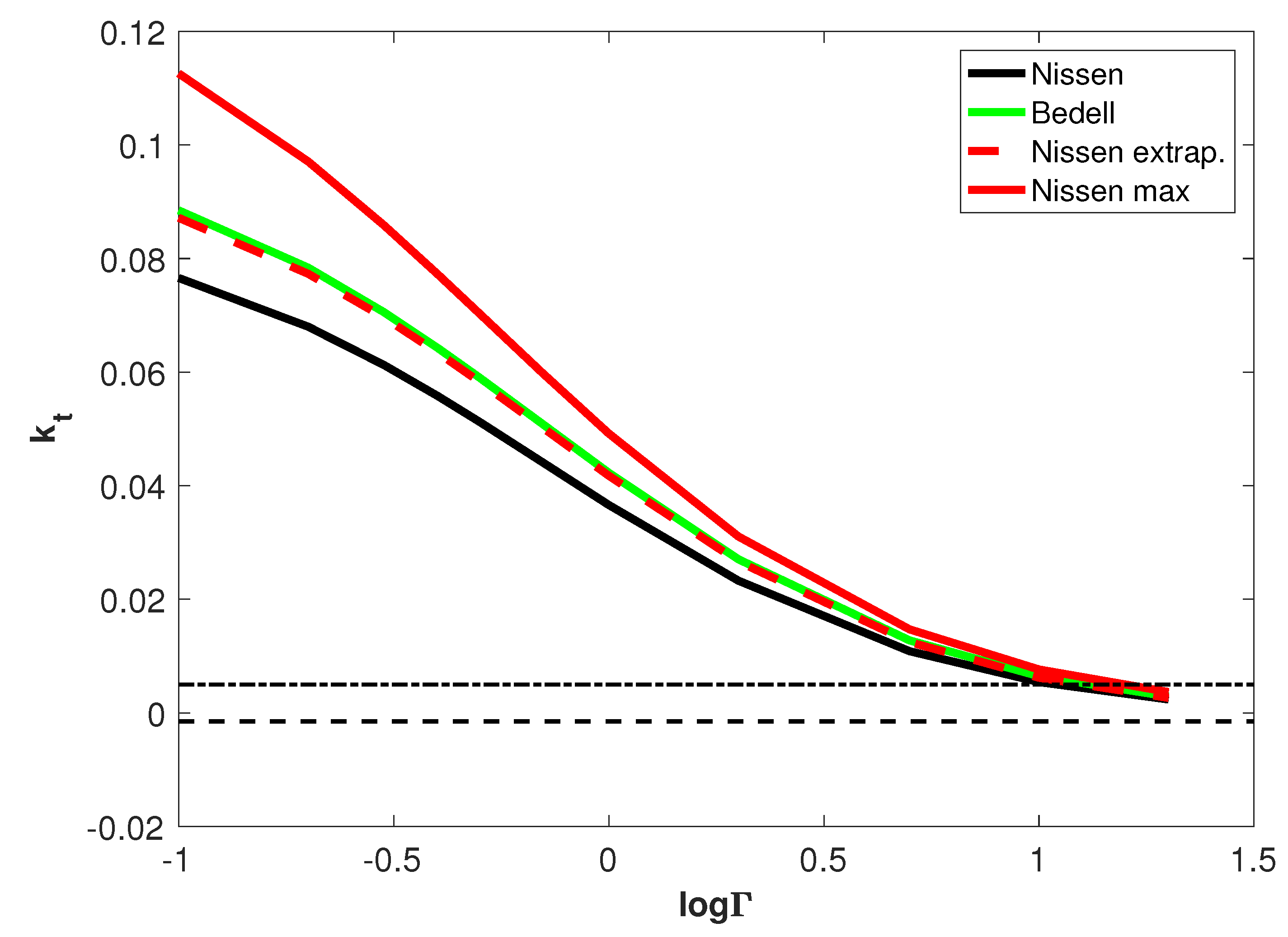
where and now mark times 2 Gyr and 9 Gyr from the start of the simulation. Examples of the dependence of on the parameters are shown in Figure 11 and Figure 12.
The two methods, using k or to determine yield parameters, are certainly not independent. They are both based on the estimates of [e/r]. Moreover, the oxygen abundance as a function of time is used in both methods, even though more indirectly so in the second, , method where it enters via the gas density estimate.
4. Application: The Origin of Carbon in the Galactic Disk
4.1. Observational Data
When applying the methods discussed above it is important to use observational data of as high quality as possible. The systematic errors in the spectrum analysis should also be minimised. Finally, the sample of stars should be selected to contain as homogeneous a population of stars as possible, not the least if the analysis is carried out with schematic single-zone models such as those used here, where the complexity of galaxy evolution is neglected. With these constraints I have selected five different sets of data:
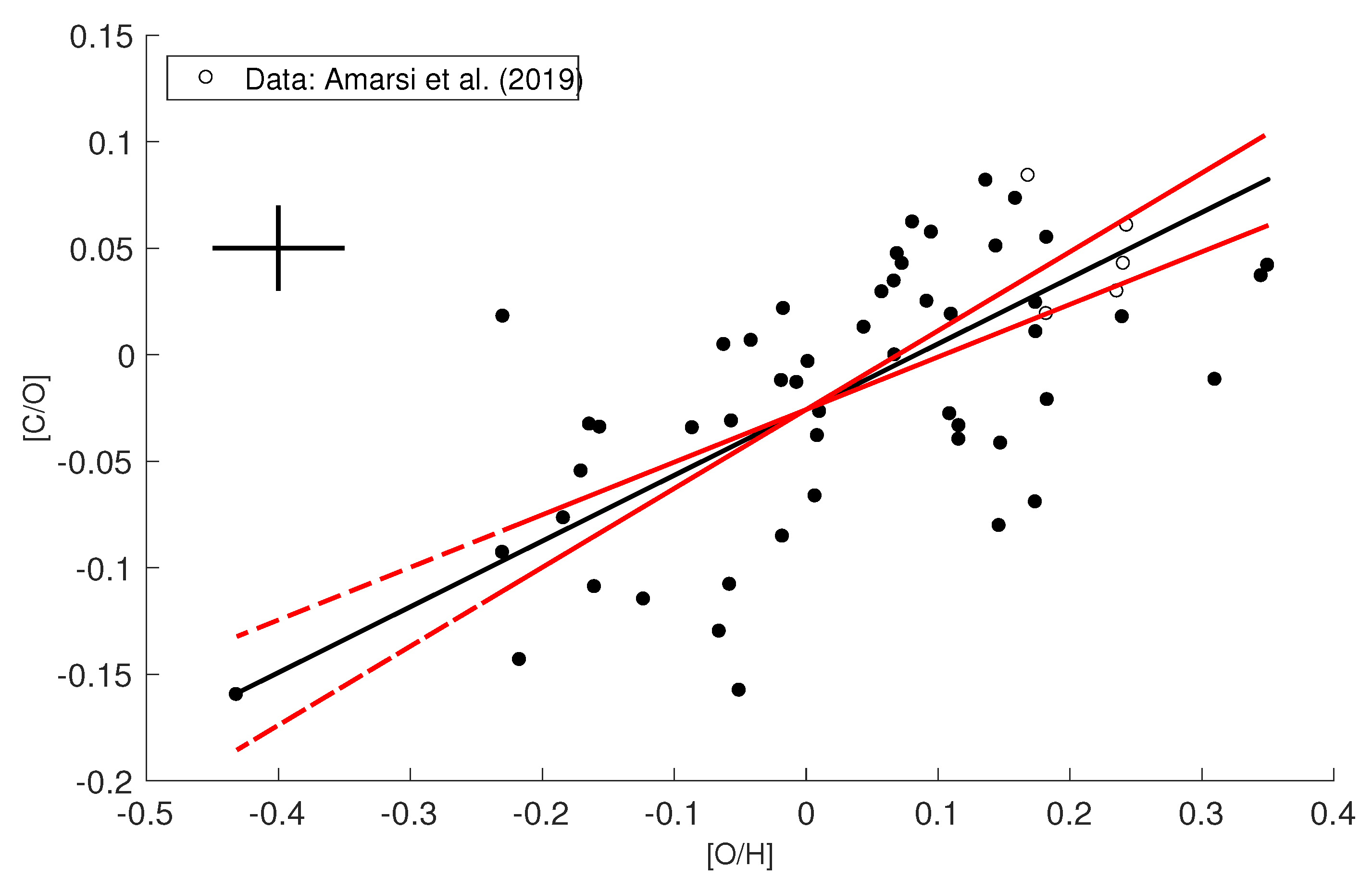
- A sample of 57 Thin disk stars from Amarsi et al. [5], see the [C/O]-[O/H] diagram in their Figure 13. Ages were not provided. Abundances were derived from high S/N spectra at high spectral resolution and with 3D model atmospheres and model spectra with due consideration of non-LTE effects. However, the slope k may be overestimated due to inclusion of some older metal-rich stars;
- The sample of 78 solar-like stars of Bedell et al. [39], see Section 3.1. Carbon abundances were derived from high-excitation C I lines and molecular CH lines with 1D LTE model atmospheres and model spectra;
- The sample of 72 solar-like stars of Nissen et al. [13] in a range of [Fe/H]. Carbon abundances were obtained from highly excited C I lines. The spectra were analysed with 1D LTE models (though with some corrections applied for 3D non-LTE effects) and the resulting abundances were judged to be rather little dependent on the uncertainties involved in the analysis of spectra. The highest [C/O] was obtained for about 10 stars with ages of about 6 Gyr with an intriguing tendency for the planetary hosts to be over-rich in carbon: These stars while the younger stars did not show any significant systematic variation of [C/O] with age;
- The sample of 67 solar-type stars of Botelho et al. [44]. Carbon abundances were obtained from molecular lines in the blue-violet spectral region and a smaller and even negative value of k was found, although there also seems to be some increase of [C/O] with time. Oxygen abundances were adopted from Bedell et al. [39], isochrone ages from Spina et al. [45];
- The sample of 365 Thin disk FGK dwarf stars of Franchini et al. [46] from the Gaia-ESO survey, with carbon abundances derived from high excitation C I lines [31], oxygen abundances from the [O I] 6300.3 Å line, and isochrone ages. Even if the errors in observed spectra and analysis may be larger for this sample than for some of the others, it has a virtue in comparison: its much bigger size and wide span in [Fe/H], extending from values around −0.5 to +0.3.
From the first four of these datasets the coefficients k and have been estimated by regressions in the [C/O] vs [C/H] plots, and [C/O] vs age plots, respectively, with due consideration of typical errors (as given by the authors) in both directions. For the Franchini et al. [46] data the values of k and were read off from their Figure 5. The resulting quantities are presented in Table 2.
The determination of these slopes is non-trivial, as is illustrated in Figure 13 and Figure 14 for two of the presently most advanced analyses [5,13]. Not unexpectedly, the results shown in Table 2 are more disparate than the formal errors suggest, which may be due to real physical scatter with mixed populations in the samples, in combination with selection effects, as well as systematic errors in the different analyses. The possibilities of handling the difficulties of scattered data and mixed populations in the samples are illustrated in the Appendix A, with results that lend some support to the error estimates for the relations deduced from the observed data. Most serious may be the fact that four of the five studies were limited to solar-like stars with a more or less limited range in [Fe/H], as pointed out by Poul Erik Nissen (private communication). Although these limits had the motivation that systematic errors in the abundance analyses and age determinations should be minimised by close differential comparisons, the main objective of the study could be at risk in that the LIMS are known to contribute much iron. If LIMS were also main contributors of C, this might result in an underestimated spread in the C abundance, with underestimates of k and . However, as in seen in Table 2, the result from the large Gaia-ESO survey by Franchini et al. [46] with its less restricted [Fe/H] range supports the results of the other studies. It seems clear that a common result is that the absolute values of the k and coefficients are relatively small. We thus estimate that the following ranges are valid for k and : and (in dex/Gyr), while values outside these limits are improbable, at least for the disk younger than the Sun. For the older disk the interesting result of Nissen et al. [13] of two separate sequences in the abundance-age diagrams (see their Figure 3 and Figure 4, and the present Figure 14) suggests a significantly steeper slope (red line: ).
4.2. Comparison with Models
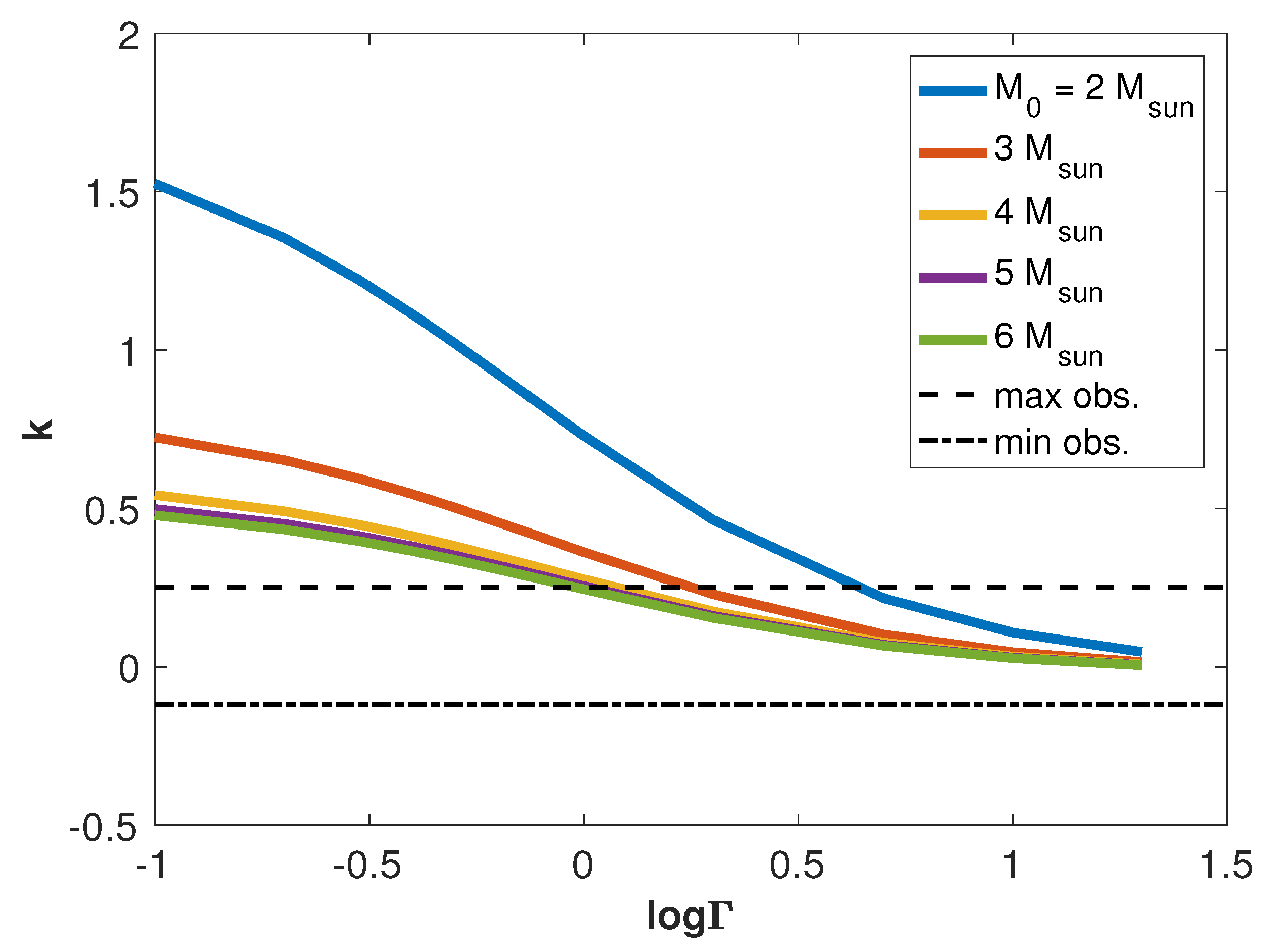
Comparing the observed k values with those of different models in Figure 8 and Figure 9 one finds that the relative contribution of carbon to the Thin disk dwarf stars from massive stars range from more than half of that provided by LIMS to complete dominance by the HMS contribution. LIMS masses of three solar masses or more seem relatively most prolific. One should, however, note that these values refer to the maximum point of the yield profile function in Equation (6). If the mass is corrected for the bias when the skewed IMF is taken into account this characteristic mass should be lowered by 0.6–0.8 solar masses.
Comparison with relations in Figure 11 and Figure 12 provides stronger constraints than those of Figure 8 and Figure 9 and suggest a contribution of carbon by HMS stars by 70% or more to the Sun. It should also be pointed out that the values are less sensitive to the time variation of the surface gas density, as is seen if Figure 12. The sensitivity to drastic changes in the initial conditions (as specified by and in Table 1) is not very significant. A reduction of by a factor of two requires a greater contribution of carbon from the LIMS in order to reach the solar value, but even then the LIMS contribution is smaller than of the total, as is seen in Figure 15. There, it is also shown that even a drastic increase in the amplitude of the variations in gas density in the “Nissen max” alternative of Figure 3 only leads to minor changes of the conclusions concerning the adequate value of , although considerable non-linear responses in the relation appear.
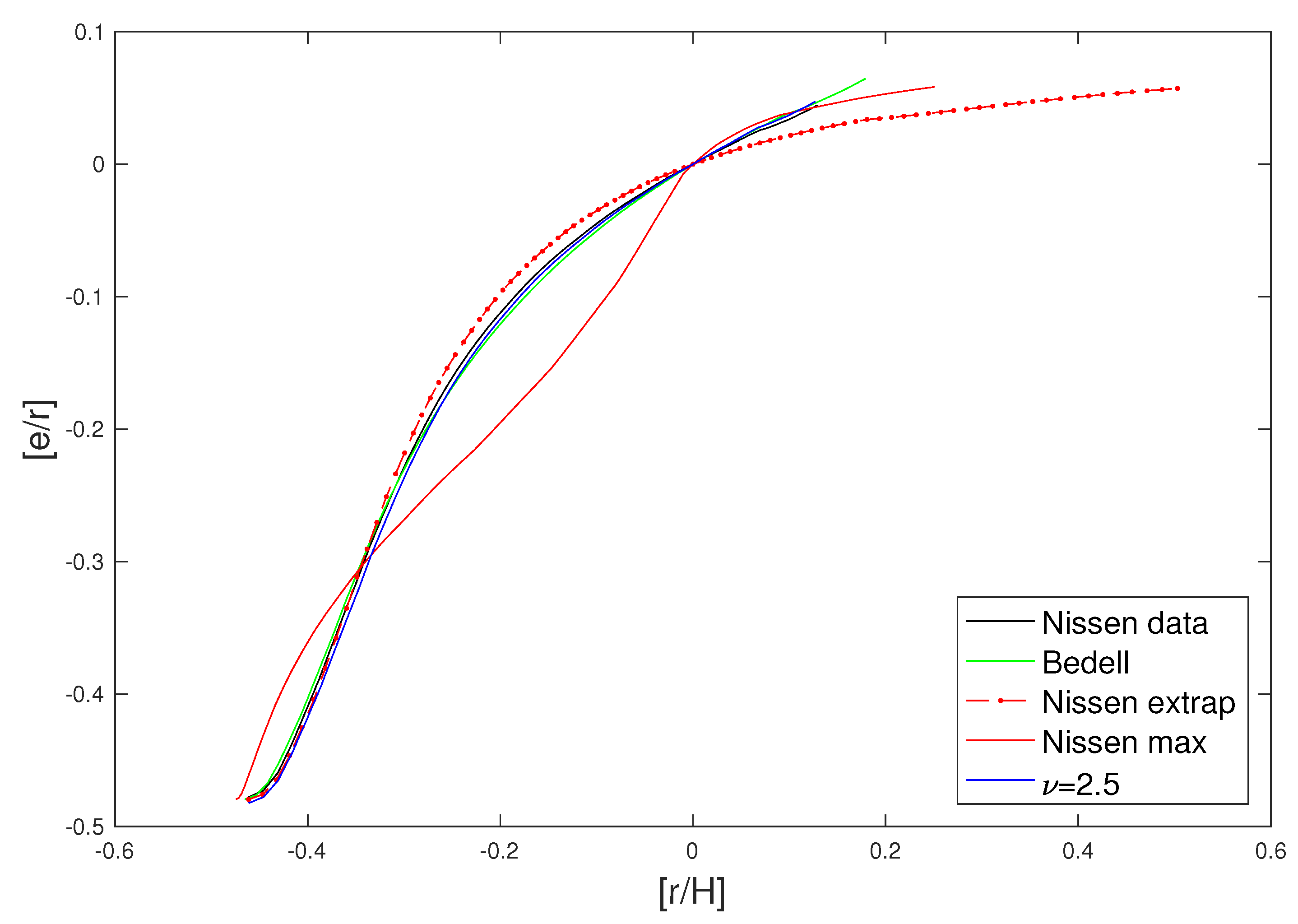
This robustness of to various uncertainties makes the great slope for the old sequence of Nissen et al. [13] in Figure 14 the more interesting. Possibly, this sequence could be the result of selection effects, for instance due to a focus in the HARPS survey (from which spectra were adopted) on high-quality spectra of planetary hosts and a consequence of the tendency of hosts to be rich in metals and carbon. However, if the two sequences really mark two different stellar populations important conclusions concerning the production of carbon may be motivated. Possible explanations, discussed by Nissen et al. [13] for the separate sequences are that two different episodes of in-falling intergalactic gas and subsequent star-formation have taken place or, alternatively, that star formation occurred earlier in the inner Galaxy, followed by migration of stars and later star-formation in the Solar neighborhood. In these two cases, and if the single-zone assumption is valid for each individual population, the slope of the red line in Figure 14 indicates that about half of the carbon in the stars in this sequence was produced by LIMS. In order to understand this, one would have to either invoke differences in the IMF, with a smaller representation of high-mass stars, or more heavy loss from the early Galactic disk by oxygen-rich winds from such stars in this early phase.
Our results are consistent with recent comparisons between model yields and extensive comparisons with observations, such as [23,31,47]. An important remaining uncertainty in our analysis is due to the simplified assumption of single-zone model of the solar neighbourhood.
I have also tentatively used the same data sources as above, which also provide accurate iron abundances, in order to derive the characteristic mass of the secondaries of the main iron providers in the Galactic disk, SNe Type Ia. The results, when comparing the data to the models used here, suggest that the dominant contributors in the Thin disk are stars with masses between 2.5 and 5 solar masses which is in good agreement with what is expected from the delay times derived for the predecessors of SN Ia (see, e.g., [48]). Attempts to also make use of the method for nitrogen indicate that more massive LIMS contribute than those that could be active for carbon. This is in accordance with current beliefs (see, e.g., [22,35]) that the more massive intermediate mass stars on the AGB convert carbon and oxygen through hot-bottom burning and via mass-loss further it to next stellar generation. However, more precise observational abundances for nitrogen are needed for this method to give interesting new results.
5. Discussion and Conclusions
As has been demonstrated above, reasonable constraints concerning yields, both as regards the relative significance of different types of stars and the masses of contributing intermediate-low mass stars, can be obtained by a relatively simple analysis of abundance–abundance-age diagrams, with little or limited theoretical a priori knowledge about the yields. One might ask whether the method may be refined, for instance by increasing the sample of stars, homogenization of the sample and further improvement of the observations and the analysis of them. In order to reach accurate results one could then go beyond a straightforward linear analysis and attempt a determination of curvature of the relations. This requires that errors in abundances are suppressed to less than 0.02 dex, at least if the sample of stars is limited to thin disk stars with their relatively small variations of abundance ratios. Comparison of stars with similar fundamental parameters is almost certainly more accurate since systematic errors in model atmospheres and calculated spectra should cancel more effectively than for stars that bridge a wider gap in the parameter space. An extension of the sample to stars in a wider [O/H] range could therefore be risky. The homogeneity of the stellar sample might also be lost, and any simple Galactic model could fail. (For instance, as is well known, the thick disk stars belong to a different population with seemingly different histories of chemical evolution). Even a sample of thin disk stars in the Solar neighbourhood may contain stars mixed in from different regions in the Galaxy, as may be indicated by the older sequence of Nissen et al. [13]. However, strict limits on the sample of stars may also introduce biasses which may lead to systematic errors in conclusions on the yields, as discussed above.
One could, however, have some hope that advantages could be gained in attempts to constrain the yields from LIMS by careful comparison between stellar populations with different characteristic time scales of formation. An obvious example is offered by the Galactic thin and thick disks, the latter which had a more rapid star formation but produced some (older) stars of similar metallicity as those in the thin disk. Since the present method is built on the differences in life times of stars with different stellar mass, one could hope that these different populations and time scales lead to differences in abundance ratios. This could then be exploited to make further conclusions about the yields. We have attempted this by using the different thin-disk populations traced by Nissen et al. [13], maybe with the different metallicities caused by an episode of strong in-fall of gas into the Galactic disk and enhanced star formation. Our results may indicate that, indeed, there were more pronounced contributions of carbon by LIMS to this population of stars. Control of selection effects of the stellar sample, and errors in the abundance measurements smaller than about 0.02 dex are, however, necessary for allowing new interesting conclusions concerning the yields. One case where this method may give significant results is for yields that are strongly metal-dependent, such as for so-called secondary elements.
Another difficulty to consider in advancing the present method is that even stars with quite similar parameters may scatter in abundance–abundance diagrams due to intrinsic scatter in chemical composition. (For instance, some such scatter is caused by the Sun, which departs systematically from most “solar twins”, stars with almost identical temperatures, masses, ages and overall metallicity [11,12]).
In spite of the various problems pointed out here the major result of the present study when applied to carbon lasts: most of the carbon in the Galactic disk, at least in the Solar neighbourhood, and in particular in the Solar System, is produced by high-mass stars.
Different additional observations may also speak in favour of this finding:
- (1)
- The suggestive agreement between observed Solar absolute abundances of oxygen and carbon and those calculated for HMS by Equation (12), on the assumption that the gas density and oxygen abundance are fairly stationary in the disk, have already been mentioned;
- (2)
- The observed C/C ratios in the photospheres of carbon stars on the AGB (Lambert et al. [49], Hinkle et al. [50]) tend to be higher than the ratios of K giants of typically 15, but in a wide range from 4 to 97, with a mean value of 48 [49]. The C/C ratios found in carbon star envelopes by Ramstedt and Olofsson [51] show a similar tendency with values in the same range, however with a distribution clearly peaked towards values below 40. The particularly C-rich carbon stars, the J-type stars, amount to at least 10% and probably considerably more of a volume-limited sample of carbon stars, see Abia et al. [52] who show that the J stars are systematically less luminous than normal N stars why they should be underrepresented in the usually magnitude-limited samples. One might then argue that the J stars should have lowered the isotope ratio to far below 50 for the solar cloud if LIMS, in particular the carbon stars, were main contributors to Solar carbon. However, Ramstedt and Olofsson [51] found that J stars tend to have significantly smaller mass-loss rates than the normal N stars why it is unclear whether the J stars could have lowered the Solar isotope ratio very much. One should also note that Ziurys et al. [53] find remarkably low isotope ratios for planetary nebulae including carbon-rich ones, ratios approximately ranging from 1 to 15. Most of these results for the isotope ratio are significantly lower than that of the Solar system of about 89 (see, e.g., Clayton and Nittler [54], Asplund et al. [40], as well as the C/C results obtained for Solar twins by Botelho et al. [44]). The production of C nuclei by HMS is several orders of magnitude smaller than the C production, according to the yields by Limongi and Chieffi [37]. These results seem to suggest that at the most about half of the carbon was produced in “typical” carbon stars, if not fractionation processes have increased the solar ratio at early stages, such as may be indicated by the findings by Smith et al. [55] of quite high carbon-isotope ratios in young stellar objects;
- (3)
- Henry et al. [56] found unexpectedly low carbon abundances in well-studied planetary nebulae with known progenitor masses of two to three solar masses, but also higher nitrogen abundances than theoretical calculations of yields suggest.
Finally, it is important to note that the relatively “theory-free” method described here to estimate yields can not replace the traditional usage of stellar models and theoretical yields, in spite of all the uncertainties involved there, not the least concerning interior mixing and mass loss. A value of the method discussed here lies in its exploratory character, as well as for verifying the results of the theoretical approach. However, it cannot, for obvious reasons, compete as regards a major and fundamental advantage of the latter method: its generation of a physical understanding of how stars work.
Funding
This research received no external funding.
Acknowledgments
Amanda Karakas is thanked for providing life times and yields for AGB stars. Anish Amarsi, Marco Limongi, Lars Mattsson and Poul Erik Nissen are thanked for important and critical comments on an earlier version of this paper. Sara Palmerini is thanked for encouragement and support, the referee of this paper for valuable suggestions, and the editors of this journal for their patience. Finally, I wish to thank Maurizio Busso, whose fundamental work led me into the fascinating field of AGB star nucleosynthsis.
Conflicts of Interest
The author declares no conflict of interest.
Abbreviations
The following abbreviations are used in this manuscript:
| AGB | Asymptotic Giant Branch |
| HMS | High Mass Stars |
| LIMS | Intermediate and Low-Mass Stars |
| IMF | Initial Mass Function (distribution over mass of stars at formation) |
Appendix A. Errors in Estimates of Slopes by Regression Analyses of Scattered Data
The effects of scatter on estimated slopes for distributions of points in the (x,y) plane were studied in the following way: First a set of x-points , distributed randomly in the interval (0,A), was generated. The corresponding set of y coordintes was generated by
where were random numbers, with gaussian distribution having a standard deviation of . These scattered points were aimed to represent the true data, free of errors, with the scatter representing physical (“cosmic”) scatter. Typically was set from 0.2 to 1.0. A regression line was then used to fit these points, which gave a slope . Next, each x- and y-coordinate was changed randomly to reflect observational errors with gaussian distributions with standard deviations of and , respectively. This was repeated M times and each time a regression line was fitted to the points, using the same procedure as that used in the main paper, where scatter in both dimensions was considered. The issue was then how well these new regression lines with slopes would retrieve the slope . Finally, the mean and the standard deviation of these slopes were calculated as measures of this fitting ability.
The parameters in this procedure were set up to match the data for the [C/O]-[O/H] diagram and the [C/O]-age diagram, respectively. The parameters were varied in order to cover the reasonable intervals.
The results are presented in Table A1.

Table A1.
Results of fits to perturbed data. Upper half: parameters set for [C/O]-[C/H] diagram of 30 stars, k. Lower part: parameters set for [C/O]-age diagram, . Left part: the starting relation was linear, Equation (A1). Right part (marked by asterisks): 15 more stars were added with values of x higher than the median value of the first set of stars, with a median y of of the maximum value of the first set and with no variation of y except for observational scatter.
| 0.0359 | 0.0148 | 0.0057 | 0.0283 | −0.0019 | 0.0048 | 0.0153 |
| 0.0700 | 0.0448 | 0.0549 | 0.0178 | 0.0495 | 0.0055 | 0.0124 |
| 0.1050 | 0.1330 | 0.1334 | 0.0178 | 0.0669 | 0.0652 | 0.0087 |
| 0.2100 | 0.1785 | 0.1747 | 0.0192 | 0.0891 | 0.1059 | 0.0104 |
| 0.2800 | 0.3389 | 0.3311 | 0.0207 | 0.1440 | 0.1417 | 0.0220 |
| 0.3500 | 0.3661 | 0.3635 | 0.0238 | 0.1536 | 0.1545 | 0.0127 |
| 0.0000 | 0.0010 | 0.0010 | 0.0027 | 0.0000 | 0.0012 | 0.0011 |
| 0.0007 | 0.0007 | 0.0025 | 0.0035 | 0.0007 | 0.0012 | 0.0009 |
| 0.0035 | 0.0032 | 0.0037 | 0.0014 | 0.0003 | 0.0001 | 0.0008 |
| 0.0042 | 0.0054 | 0.0050 | 0.0020 | 0.0014 | 0.0014 | 0.0007 |
| 0.0056 | 0.0089 | 0.0083 | 0.0021 | 0.0027 | 0.0032 | 0.0011 |
| 0.0070 | 0.0111 | 0.0109 | 0.0016 | 0.0072 | 0.0069 | 0.0012 |
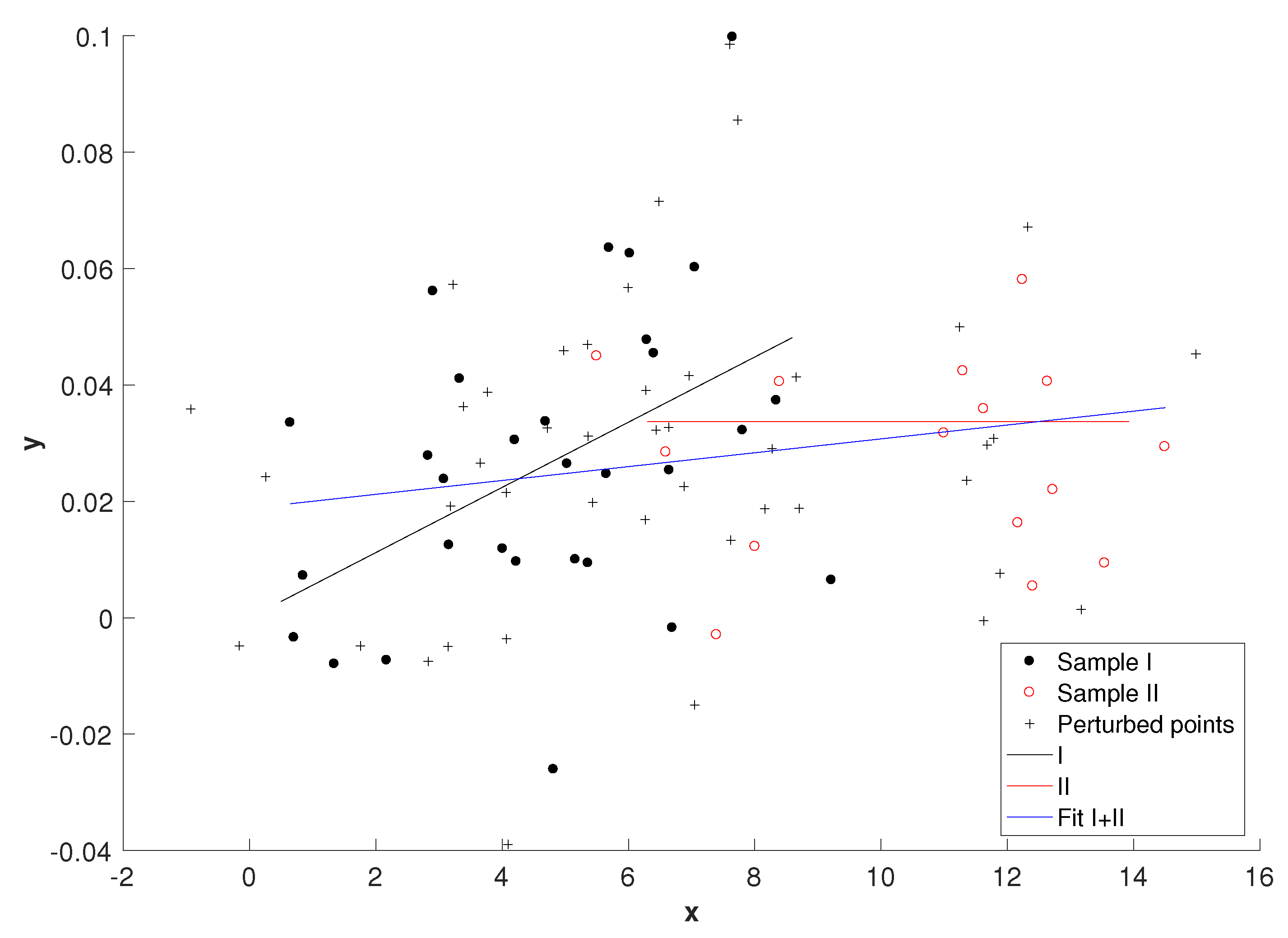
In order to explore the sensitivity of the results to the starting assumption of a linear relation, to which perturbations were added which roughly leads to a symmetric distribution of points around the line, experiments have also been made where the relation was broken by adding another “population” of points to the analysis, comprising one third of the points with no systematic slope of y versus x, and all only represented in half of the total x interval as is illustrated in Figure A1. These arrangements were inspired by the tendencies for some of the observed abundance–abundance diagrams to show such signs of several stellar populations. One example of the effects of such a two-population sample is shown in the right part of Table A1.
It is seen that the standard deviations are relatively constant and not very dependent of for a given set of characteristic plot parameters. The addition of the second population did not increase the standard deviations, sooner they tend to get smaller as the slope of the line fitted to all points in the diagram gets more restricted by the added population. The standard deviations in the slopes are consistent with the errors estimated in Section 4.1. These results support the procedure which has been used to trace the tendencies in the observed diagrams in the present study.
Figure A1.
An example of the simple experiments with results presented in Table A1. Here first 30 points (“Sample I”) were placed along a line (black), were then moved randomly in x by with a standard deviation units to the positions of the black dots. 15 more point (“Sample II”, red circles) were placed along a horizontal line, red line, and then moved randomly in x as for Sample I. Next, all points were given “observational scatter”, with and units, to positions denoted by crosses. Finally, these points were fitted by a regresson line, blue in the figure with the slope . The procedure was repeated ten times and and were calculated.

References
- Wallerstein, G. Nucleogenesis Clues Derived from the Composition of G Dwarfs. Astron. J. 1962, 67, 122. [Google Scholar] [CrossRef]
- Tinsley, B.M. Stellar lifetimes and abundance ratios in chemical evolution. Astrophys. J. 1979, 229, 1046–1056. [Google Scholar] [CrossRef]
- Edvardsson, B.; Andersen, J.; Gustafsson, B.; Lambert, D.L.; Nissen, P.E.; Tomkin, J. The Chemical Evolution of the Galactic Disk—Part One—Analysis and Results. Astron. Astrophys. 1993, 275, 101. [Google Scholar]
- Bensby, T.; Feltzing, S.; Oey, M.S. Exploring the Milky Way stellar disk. A detailed elemental abundance study of 714 F and G dwarf stars in the solar neighbourhood. Astron. Astrophys. 2014, 562, A71. [Google Scholar] [CrossRef]
- Amarsi, A.M.; Nissen, P.E.; Skúladóttir, Á. Carbon, oxygen, and iron abundances in disk and halo stars. Implications of 3D non-LTE spectral line formation. Astron. Astrophys. 2019, 630, A104. [Google Scholar] [CrossRef] [Green Version]
- Randich, S.; Gilmore, G.; Gaia-ESO Consortium. The Gaia-ESO Large Public Spectroscopic Survey. Messenger 2013, 154, 47–49. [Google Scholar]
- Wilson, J.C.; Hearty, F.; Skrutskie, M.F.; Majewski, S.R.; Schiavon, R.; Eisenstein, D.; Gunn, J.; Holtzman, J.; Nidever, D.; Gillespie, B.; et al. Performance of the Apache Point Observatory Galactic Evolution Experiment (APOGEE) high-resolution near-infrared multi-object fiber spectrograph. In Proceedings of the Ground-Based and Airborne Instrumentation for Astronomy IV; McLean, I.S., Ramsay, S.K., Takami, H., Eds.; Society of Photo-Optical Instrumentation Engineers (SPIE) Conference Series; SPIE: Bellingham, DC, USA, 2012; Volume 8446, p. 84460H. [Google Scholar] [CrossRef]
- De Silva, G.M.; Freeman, K.C.; Bland-Hawthorn, J.; Martell, S.; de Boer, E.W.; Asplund, M.; Keller, S.; Sharma, S.; Zucker, D.B.; Zwitter, T.; et al. The GALAH survey: Scientific motivation. Mon. Not. R. Astron. Soc. 2015, 449, 2604–2617. [Google Scholar] [CrossRef] [Green Version]
- Zhao, G.; Zhao, Y.H.; Chu, Y.Q.; Jing, Y.P.; Deng, L.C. LAMOST spectral survey—An overview. Res. Astron. Astrophys. 2012, 12, 723–734. [Google Scholar] [CrossRef] [Green Version]
- Asplund, M. New Light on Stellar Abundance Analyses: Departures from LTE and Homogeneity. Annu. Rev. Astron. Astrophys. 2005, 43, 481–530. [Google Scholar] [CrossRef]
- Nissen, P.E.; Gustafsson, B. High-precision stellar abundances of the elements: Methods and applications. Astron. Astrophys. Rev. 2018, 26, 6. [Google Scholar] [CrossRef] [Green Version]
- Meléndez, J.; Asplund, M.; Gustafsson, B.; Yong, D. The Peculiar Solar Composition and Its Possible Relation to Planet Formation. Astrophys. J. 2009, 704, L66–L70. [Google Scholar] [CrossRef] [Green Version]
- Nissen, P.E.; Christensen-Dalsgaard, J.; Mosumgaard, J.R.; Silva Aguirre, V.; Spitoni, E.; Verma, K. High-precision abundances of elements in solar-type stars. Evidence of two distinct sequences in abundance-age relations. Astron. Astrophys. 2020, 640, A81. [Google Scholar] [CrossRef]
- Schmidt, M. The Rate of Star Formation. Astrophys. J. 1959, 129, 243. [Google Scholar] [CrossRef]
- Salpeter, E.E. The Luminosity Function and Stellar Evolution. Astrophys. J. 1955, 121, 161. [Google Scholar] [CrossRef]
- Truran, J.W.; Cameron, A.G.W. Evolutionary Models of Nucleosynthesis in the Galaxy. Int. Astron. Union Colloq. 1971, 14, 179–222. [Google Scholar] [CrossRef] [Green Version]
- Lynden-Bell, D. The chemical evolution of galaxies. Vistas Astron. 1975, 19, 299–316. [Google Scholar] [CrossRef] [Green Version]
- Pagel, B.E.J.; Patchett, B.E. Metal abundances in nearby stars and the chemical history of the solar neighbourhood. Mon. Not. R. Astron. Soc. 1975, 172, 13–40. [Google Scholar] [CrossRef]
- Tinsley, B.M. Evolution of the Stars and Gas in Galaxies. Astrophys. J. 1980, 5, 287–388. [Google Scholar] [CrossRef]
- Matteucci, F. Modelling the chemical evolution of the Milky Way. Astron. Astrophys. Rev. 2021, 29, 5. [Google Scholar] [CrossRef]
- Meynet, G.; Maeder, A. Stellar evolution with rotation. VIII. Models at Z = 10−5 and CNO yields for early galactic evolution. Astron. Astrophys. 2002, 390, 561–583. [Google Scholar] [CrossRef] [Green Version]
- Busso, M.; Gallino, R.; Wasserburg, G.J. Nucleosynthesis in Asymptotic Giant Branch Stars: Relevance for Galactic Enrichment and Solar System Formation. Annu. Rev. Astron. Astrophys. 1999, 37, 239–309. [Google Scholar] [CrossRef] [Green Version]
- Karakas, A.I.; Lattanzio, J.C. The Dawes Review 2: Nucleosynthesis and Stellar Yields of Low- and Intermediate-Mass Single Stars. Publ. Astron. Soc. Aust. 2014, 31, e030. [Google Scholar] [CrossRef] [Green Version]
- Gustafsson, B.; Karlsson, T.; Olsson, E.; Edvardsson, B.; Ryde, N. The origin of carbon, investigated by spectral analysis of solar-type stars in the Galactic Disk. Astron. Astrophys. 1999, 342, 426–439. [Google Scholar]
- Henry, R.B.C.; Edmunds, M.G.; Köppen, J. On the Cosmic Origins of Carbon and Nitrogen. Astrophys. J. 2000, 541, 660–674. [Google Scholar] [CrossRef] [Green Version]
- Chiappini, C.; Matteucci, F.; Meynet, G. Stellar yields with rotation and their effect on chemical evolution models. Astron. Astrophys. 2003, 410, 257–267. [Google Scholar] [CrossRef] [Green Version]
- Chiappini, C.; Romano, D.; Matteucci, F. Oxygen, carbon and nitrogen evolution in galaxies. Mon. Not. R. Astron. Soc. 2003, 339, 63–81. [Google Scholar] [CrossRef] [Green Version]
- Bensby, T.; Feltzing, S. The origin and chemical evolution of carbon in the Galactic thin and thick discs. Mon. Not. R. Astron. Soc. 2006, 367, 1181–1193. [Google Scholar] [CrossRef] [Green Version]
- Mattsson, L. The origin of carbon revisited: Winds of carbon-stars. Phys. Scr. 2008, 133, 014027. [Google Scholar] [CrossRef]
- Griffith, E.; Johnson, J.A.; Weinberg, D.H. Abundance Ratios in GALAH DR2 and Their Implications for Nucleosynthesis. Astrophys. J. 2019, 886, 84. [Google Scholar] [CrossRef]
- Franchini, M.; Morossi, C.; Di Marcantonio, P.; Chavez, M.; Adibekyan, V.Z.; Bayo, A.; Bensby, T.; Bragaglia, A.; Calura, F.; Duffau, S.; et al. The Gaia-ESO Survey: Carbon Abundance in the Galactic Thin and Thick Disks. Astrophys. J. 2020, 888, 55. [Google Scholar] [CrossRef] [Green Version]
- Randich, S.; Magrini, L. Light elements in the Universe. Front. Astron. Space Sci. 2021, 8, 6. [Google Scholar] [CrossRef]
- Kroupa, P. On the variation of the initial mass function. Mon. Not. R. Astron. Soc. 2001, 322, 231–246. [Google Scholar] [CrossRef]
- Kennicutt, R.C.; Evans, N.J. Star Formation in the Milky Way and Nearby Galaxies. Annu. Rev. Astron. Astrophys. 2012, 50, 531–608. [Google Scholar] [CrossRef] [Green Version]
- Karakas, A.I.; Lugaro, M. Stellar Yields from Metal-rich Asymptotic Giant Branch Models. Astrophys. J. 2016, 825, 26. [Google Scholar] [CrossRef]
- Karakas, A.I.; Lugaro, M.; Carlos, M.; Cseh, B.; Kamath, D.; García-Hernández, D.A. Heavy-element yields and abundances of asymptotic giant branch models with a Small Magellanic Cloud metallicity. Mon. Not. R. Astron. Soc. 2018, 477, 421–437. [Google Scholar] [CrossRef]
- Limongi, M.; Chieffi, A. VizieR Online Data Catalog: Models and yields of 13-120Mȯ massive stars (Limongi+. VizieR Online Data Catalog 2018, J/ApJS/237/13. [Google Scholar] [CrossRef]
- McKee, C.F.; Parravano, A.; Hollenbach, D.J. Stars, Gas, and Dark Matter in the Solar Neighborhood. Astrophys. J. 2015, 814, 13. [Google Scholar] [CrossRef] [Green Version]
- Bedell, M.; Bean, J.L.; Melendez, J.; Spina, L.; Ramirez, I.; Asplund, M.; Alves-Brito, A.; dos Santos, L.; Dreizler, S.; Yong, D.; et al. The Chemical Homogeneity of Sun-like Stars in the Solar Neighborhood. arXiv 2018, arXiv:1802.02576. [Google Scholar] [CrossRef] [Green Version]
- Asplund, M.; Amarsi, A.M.; Grevesse, N. The chemical make-up of the Sun: A 2020 vision. Astron. Astrophys. 2021, 653, A141. [Google Scholar] [CrossRef]
- Sahlholdt, C.L.; Feltzing, S.; Lindegren, L.; Church, R.P. Benchmark ages for the Gaia benchmark stars. Mon. Not. R. Astron. Soc. 2019, 482, 895–920. [Google Scholar] [CrossRef] [Green Version]
- Silva Aguirre, V.; Lund, M.N.; Antia, H.M.; Ball, W.H.; Basu, S.; Christensen-Dalsgaard, J.; Lebreton, Y.; Reese, D.R.; Verma, K.; Casagrande, L.; et al. Standing on the Shoulders of Dwarfs: The Kepler Asteroseismic LEGACY Sample. II.Radii, Masses, and Ages. Astrophys. J. 2017, 835, 173. [Google Scholar] [CrossRef] [Green Version]
- Silva Aguirre, V.; Bojsen-Hansen, M.; Slumstrup, D.; Casagrande, L.; Kawata, D.; Ciucă, I.; Handberg, R.; Lund, M.N.; Mosumgaard, J.R.; Huber, D.; et al. Confirming chemical clocks: Asteroseismic age dissection of the Milky Way disc(s). Mon. Not. R. Astron. Soc. 2018, 475, 5487–5500. [Google Scholar] [CrossRef] [Green Version]
- Botelho, R.B.; Milone, A.d.C.; Meléndez, J.; Alves-Brito, A.; Spina, L.; Bean, J.L. Carbon, isotopic ratio 12C/13C, and nitrogen in solar twins: Constraints for the chemical evolution of the local disc. Mon. Not. R. Astron. Soc. 2020, 499, 2196–2213. [Google Scholar] [CrossRef]
- Spina, L.; Meléndez, J.; Karakas, A.I.; Ramírez, I.; Monroe, T.R.; Asplund, M.; Yong, D. Nucleosynthetic history of elements in the Galactic disk. [X/Fe]-age relations from high-precision spectroscopy. Astron. Astrophys. 2016, 593, A125. [Google Scholar] [CrossRef] [Green Version]
- Franchini, M.; Morossi, C.; Di Marcantonio, P.; Chavez, M.; Adibekyan, V.; Bensby, T.; Bragaglia, A.; Gonneau, A.; Heiter, U.; Kordopatis, G.; et al. The Gaia-ESO Survey: Oxygen Abundance in the Galactic Thin and Thick Disks. Astron. J. 2021, 161, 9. [Google Scholar] [CrossRef]
- Jofré, P.; Jackson, H.; Tucci Maia, M. Traits for chemical evolution in solar twins. Trends of neutron-capture elements with stellar age. Astron. Astrophys. 2020, 633, L9. [Google Scholar] [CrossRef] [Green Version]
- Freundlich, J.; Maoz, D. The delay time distribution of Type-Ia supernovae in galaxy clusters: The impact of extended star-formation histories. Mon. Not. R. Astron. Soc. 2021, 502, 5882–5895. [Google Scholar] [CrossRef]
- Lambert, D.L.; Gustafsson, B.; Eriksson, K.; Hinkle, K.H. The Chemical Composition of Carbon Stars. I. Carbon, Nitrogen, and Oxygen in 30 Cool Carbon Stars in the Galactic Disk. Astrophys. J. Suppl. Ser. 1986, 62, 373. [Google Scholar] [CrossRef]
- Hinkle, K.H.; Lebzelter, T.; Straniero, O. Carbon and Oxygen Isotopic Ratios for Nearby Miras. Astrophys. J. 2016, 825, 38. [Google Scholar] [CrossRef] [Green Version]
- Ramstedt, S.; Olofsson, H. The 12CO/13CO ratio in AGB stars of different chemical type. Connection to the 12C/13C ratio and the evolution along the AGB. Astron. Astrophys. 2014, 566, A145. [Google Scholar] [CrossRef] [Green Version]
- Abia, C.; de Laverny, P.; Romero, M.; Figueras, F. Characterisation of Galactic carbon stars and related stars from Gaia-EDR3. arXiv 2022, arXiv:2206.00405. [Google Scholar] [CrossRef]
- Ziurys, L.M.; Schmidt, D.R.; Woolf, N.J. Carbon Isotope Ratios in Planetary Nebulae: The Unexpected Enhancement of 13C. Astrophys. J. 2020, 900, L31. [Google Scholar] [CrossRef]
- Clayton, D.D.; Nittler, L.R. Astrophysics with Presolar Stardust. Annu. Rev. Astron. Astrophys. 2004, 42, 39–78. [Google Scholar] [CrossRef] [Green Version]
- Smith, R.L.; Pontoppidan, K.M.; Young, E.D.; Morris, M.R. Observational Signatures of 12CO-13CO Partitioning in Ice and Gas Towards Local Young Stellar Objects and Molecular Clouds. Mol. Univ. 2011, 280, 341. [Google Scholar]
- Henry, R.B.C.; Stephenson, B.G.; Miller Bertolami, M.M.; Kwitter, K.B.; Balick, B. On the production of He, C, and N by low- and intermediate-mass stars: A comparison of observed and model-predicted planetary nebula abundances. Mon. Not. R. Astron. Soc. 2018, 473, 241–260. [Google Scholar] [CrossRef] [Green Version]
Figure 1.
Examples of different profiles of yields for AGB stars at different metallicities Z, plotted as functions of the initial masses of the stars (open and filled circles). For the meaning of the parameters, see the text. Theoretical carbon yields from Karakas and Lugaro [35] are also plotted.
Figure 1.
Examples of different profiles of yields for AGB stars at different metallicities Z, plotted as functions of the initial masses of the stars (open and filled circles). For the meaning of the parameters, see the text. Theoretical carbon yields from Karakas and Lugaro [35] are also plotted.

Figure 2.
Observed oxygen abundances versus age estimates according to Nissen et al. [13]. Typical mean errors are indicated by the cross. Different tentative relations are also shown (see text).
Figure 2.
Observed oxygen abundances versus age estimates according to Nissen et al. [13]. Typical mean errors are indicated by the cross. Different tentative relations are also shown (see text).

Figure 3.
The surface density in the Galactic disk, as a function of time was estimated by means of Equation (5) from the observed oxygen abundances obtained by Nissen et al. [13] and Bedell et al. [39]. Regression lines and the different free drawn lines in Figure 2 were used and the results are indicated by curves in corresponding colours.

Figure 4.
The calculated variation of the abundance [e/r] relative to [r/H] for different values of : From bottom to top = 2, 3, 4, 5, and 6 M. The black full lines represent results for LIMS peak profiles with a width of 2 M, the red dashed curves correspond to results with = 1 . g = 0.5 in all cases.

Figure 5.
The effects of introducing metallicity-dependent yields on the |e/r[-| r/H] diagram. All curves represent runs with = 3 , with = 2 M and with a solar carbon contribution from massive stars of of that of LIMS. . Full black line: , full red line: , dashed red line: , cyan line: .
Figure 5.
The effects of introducing metallicity-dependent yields on the |e/r[-| r/H] diagram. All curves represent runs with = 3 , with = 2 M and with a solar carbon contribution from massive stars of of that of LIMS. . Full black line: , full red line: , dashed red line: , cyan line: .

Figure 6.
The effects on the abundance–abundance diagram of varying the contribution of massive stars relative to that of intermediate mass stars, , to the solar abundance of element “e”. The curves correspond, from top to bottom, to g = 20, 5, 2, 1.6, 1.4, 1.2, 1.0, 0.8, 0.6 0.4, 0.2, and 0.1, respectively, in relative contributions. All curves represent runs with = 3 and M, and metallicity independent yields.

Figure 7.
The effects on the abundance–abundance diagram of changes of the gas surface density as a function of time, according to the different results displayed in Figure 3. The effect of changing the exponent of the IMF from a value of 2.3 to 2.5 is also shown. for all results shown.
Figure 7.
The effects on the abundance–abundance diagram of changes of the gas surface density as a function of time, according to the different results displayed in Figure 3. The effect of changing the exponent of the IMF from a value of 2.3 to 2.5 is also shown. for all results shown.

Figure 8.
The effects on the slope k of the [r/H]-[e/r] relation of varying . The upper and lower limits of the observed slopes for e = carbon and r = oxygen are indicated by dashed horizontal lines, see Section 4.1.
Figure 8.
The effects on the slope k of the [r/H]-[e/r] relation of varying . The upper and lower limits of the observed slopes for e = carbon and r = oxygen are indicated by dashed horizontal lines, see Section 4.1.

Figure 9.
The effects on the slope k of the [r/H]-[e/r] relation of varying different parameters of the yield profile of the LIMS. The upper and lower limits of the observed slopes for e = carbon and r = oxygen are indicated by dashed horizontal lines, see further Section 4.1.
Figure 9.
The effects on the slope k of the [r/H]-[e/r] relation of varying different parameters of the yield profile of the LIMS. The upper and lower limits of the observed slopes for e = carbon and r = oxygen are indicated by dashed horizontal lines, see further Section 4.1.

Figure 10.
The relations between time and [e/r] for different sets of parameters. Full black lines from bottom to top: = 2, 3, 4, 5 and 6 M, all with M; dashed lines: = 1 M, = 2, 3 M; dashed-dotted lines: 0.6 M, = 2, 3 M, = 2 M; red line: = 1 M, = 3 M, = 2 M, 0 M.
Figure 10.
The relations between time and [e/r] for different sets of parameters. Full black lines from bottom to top: = 2, 3, 4, 5 and 6 M, all with M; dashed lines: = 1 M, = 2, 3 M; dashed-dotted lines: 0.6 M, = 2, 3 M, = 2 M; red line: = 1 M, = 3 M, = 2 M, 0 M.

Figure 11.
The effects on the slope of the [e/r]-time relation of varying . The upper and lower limits of the observed slopes for e = carbon and r = oxygen are indicated by dashed horizontal lines, see text.
Figure 11.
The effects on the slope of the [e/r]-time relation of varying . The upper and lower limits of the observed slopes for e = carbon and r = oxygen are indicated by dashed horizontal lines, see text.

Figure 12.
The effects on the slope of the [e/r]-time relation of the selection of data for estimating the surface gas density. . The upper and lower limits of the observed slopes for carbon/oxygen are indicated by dashed horizontal lines, see text.
Figure 12.
The effects on the slope of the [e/r]-time relation of the selection of data for estimating the surface gas density. . The upper and lower limits of the observed slopes for carbon/oxygen are indicated by dashed horizontal lines, see text.

Figure 13.
The observed oxygen and carbon abundances of Galactic Thin-disk stars from Amarsi et al. [5]. The stars with abundances denoted by open circles are relatively old metal-rich stars, which may be suspected to have their origin in the inner Galaxy. The three lines represent, with increased slope, a regression line with due consideration of estimated errors in both directions (see cross), and slopes of respectively 25% and 50% greater than that of the regression line.The difficulties in safely measuring the slope and the curvature of the relation, are obvious.

Figure 14.
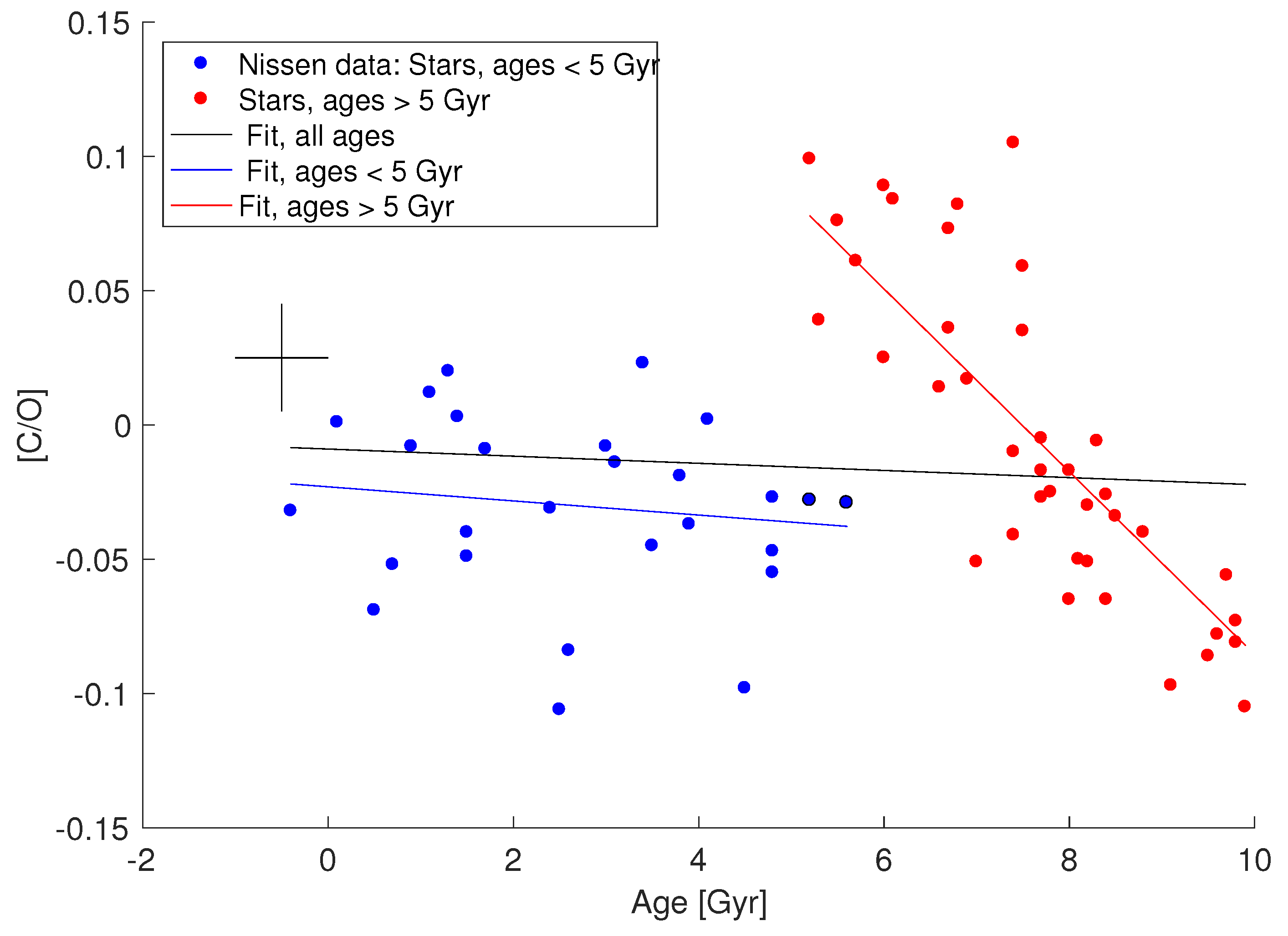
The observed oxygen and carbon abundances of Galactic stars from Nissen et al. [13]. The stars with abundances denoted by red dots are relatively old metal-rich stars, many of which may be suspected to have their origin in the inner Galaxy. As pointed out in [13] most of these stars with high [C/O] are known to be planetary hosts. The three lines represent regression lines with due consideration of estimated errors in both directions (see cross), the long black line for all stars, the blue line for the stars with ages smaller than 5 Gyr + two more stars (points encircled in black), and the red line the stars older than 5 Gyr. The slopes inserted in Table 2 are those of the first and second line. For the red line, see text.
Figure 14.
The observed oxygen and carbon abundances of Galactic stars from Nissen et al. [13]. The stars with abundances denoted by red dots are relatively old metal-rich stars, many of which may be suspected to have their origin in the inner Galaxy. As pointed out in [13] most of these stars with high [C/O] are known to be planetary hosts. The three lines represent regression lines with due consideration of estimated errors in both directions (see cross), the long black line for all stars, the blue line for the stars with ages smaller than 5 Gyr + two more stars (points encircled in black), and the red line the stars older than 5 Gyr. The slopes inserted in Table 2 are those of the first and second line. For the red line, see text.

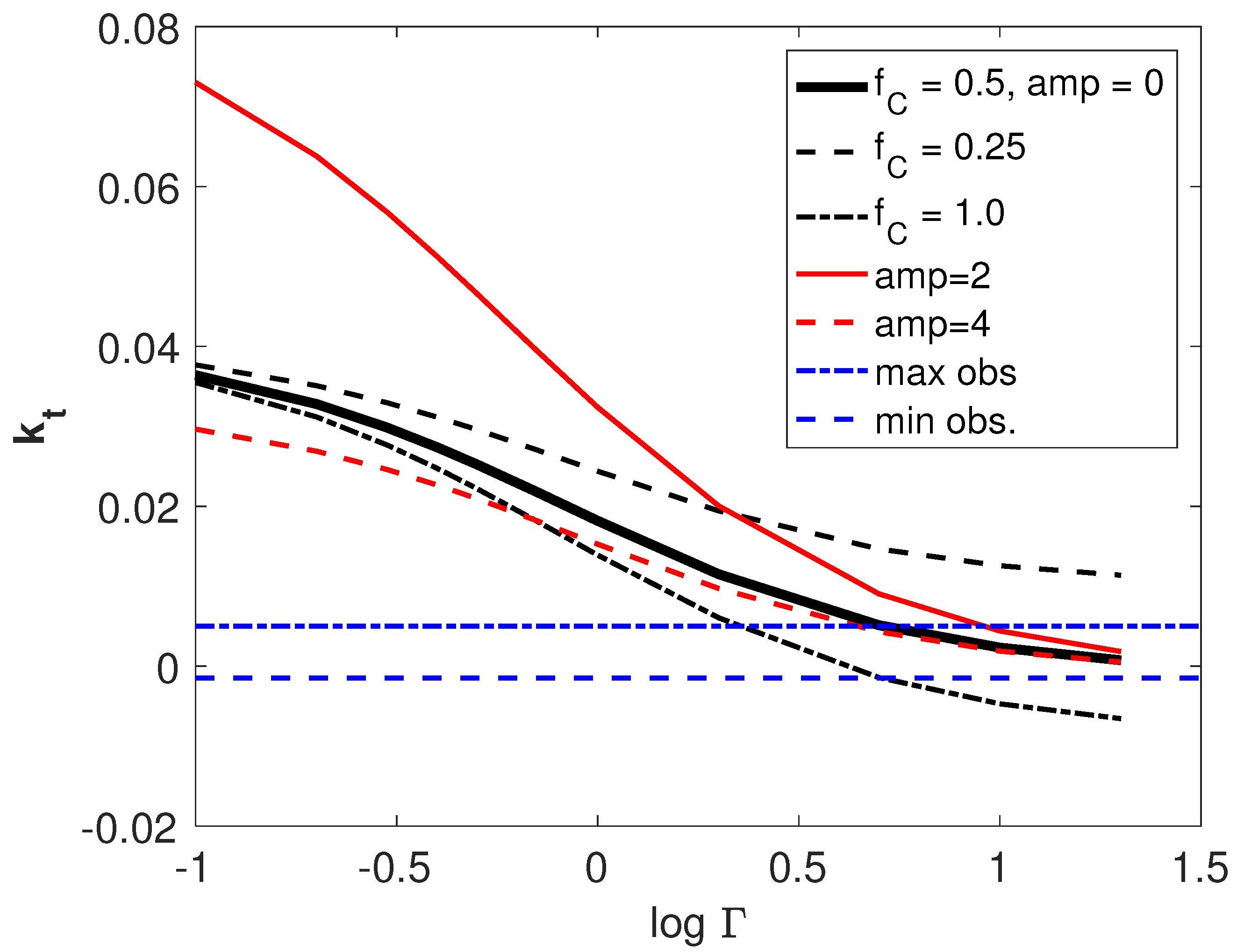
Figure 15.
The effects on the slope of the [e/r]-time relation when changing the initial condition for the reference element (black curves) and increasing the amplitude in the gas density oscillations (as obtained from the “Nissen max” oxygen abundances), by a factor of 2 and 4, respectively (red curves). The upper and lower limits of the observed slopes are indicated by dashed horizontal lines, see text.

Table 1.
Model parameters.
| Parameter | Symbol | Equation | Values 1 |
|---|---|---|---|
| Galaxy | |||
| IMF mass dependence | (2) | 2.2, 2.35, 2.5 | |
| Star formation rate | (3) | 1.2, 1.4, 1.6 | |
| Yield | |||
| Peak mass of profile | (6), (7), (9) | 1, 2, 3, 4, 5, 6 | |
| Width of peak | (6), (7), (10) | 1, 2 | |
| Extension to high mass | Q | (8) | 0.0–0.6 |
| Z correction to | (9) | 0, 1 | |
| Z correction to | (10) | 0, 1 | |
| Z correction to HMS yield | (11) | 0.0–1.0 | |
| Contribution of HMS rel. to LIMS in Sun | g | 0.1–1.0–20 | |
| Initial conditions | |||
| Initial O and C abundances | 0.25–0.5–1.0 |
1 Standard choices of parameters are underlined.
Publisher’s Note: MDPI stays neutral with regard to jurisdictional claims in published maps and institutional affiliations. |
© 2022 by the author. Licensee MDPI, Basel, Switzerland. This article is an open access article distributed under the terms and conditions of the Creative Commons Attribution (CC BY) license (https://creativecommons.org/licenses/by/4.0/).
Share and Cite
MDPI and ACS Style
Gustafsson, B. Chemical Tracing and the Origin of Carbon in the Galactic Disk. Universe 2022, 8, 409. https://0-doi-org.brum.beds.ac.uk/10.3390/universe8080409
AMA Style
Gustafsson B. Chemical Tracing and the Origin of Carbon in the Galactic Disk. Universe. 2022; 8(8):409. https://0-doi-org.brum.beds.ac.uk/10.3390/universe8080409
Chicago/Turabian StyleGustafsson, Bengt. 2022. "Chemical Tracing and the Origin of Carbon in the Galactic Disk" Universe 8, no. 8: 409. https://0-doi-org.brum.beds.ac.uk/10.3390/universe8080409
Note that from the first issue of 2016, this journal uses article numbers instead of page numbers. See further details here.