Magic Wavelengths for Optical-Lattice Based Cs and Rb Active Clocks


1
Department of Physics, Guru Nanak Dev University, Amritsar, Punjab 143005, India
2
Atomic, Molecular and Optical Physics Division, Physical Research Laboratory, Navrangpura, Ahmedabad 380009, India
3
Beijing National Laboratory for Condensed Matter Physics, Institute of Physics, Chinese Academy of Sciences, Beijing 100190, China
4
University of Chinese Academy of Sciences, Beijing 100049, China
*
Author to whom correspondence should be addressed.
Atoms 2020, 8(4), 79; https://0-doi-org.brum.beds.ac.uk/10.3390/atoms8040079
Submission received: 28 September 2020
/
Revised: 2 November 2020
/
Accepted: 3 November 2020
/
Published: 10 November 2020
Abstract
:Active clocks could provide better stabilities during initial stages of measurements over passive clocks, in which stabilities become saturated only after long-term measurements. This unique feature of an active clock has led to search for suitable candidates to construct such clocks. The other challenging task of an atomic clock is to reduce its possible systematics. A major part of the optical lattice atomic clocks based on neutral atoms are reduced by trapping atoms at the magic wavelengths of the optical lattice lasers. Keeping this in mind, we find the magic wavelengths between all possible hyperfine levels of the transitions in Rb and Cs atoms that were earlier considered to be suitable for making optical active clocks. To validate the results, we give the static dipole polarizabilities of Rb and Cs atoms using the electric dipole transition amplitudes that are used to evaluate the dynamic dipole polarizabilities and compare them with the available literature values.
1. Introduction
The future definition of second in the International System of Units (SI) requires the realization of ultraprecise, narrow and concise form of clocks. Active clocks are expected to achieve better short-term stabilities [1] against the available optical clocks when a hybrid clock system consisting of the proposed active clock and an appropriate passive clock are designed together. Such a hybrid system is expected to cater both the short- and long-term stabilities to an indigenous frequency standard. Therefore, active clocks can serve as conducive time keeping standard at the short-term time scale. The output frequency of an active clock is determined by an atomic transition in perturbation-free environment. Proposed more than a decade ago, active optical clocks thus offer a possible solution to the bottleneck of accomplishing high stabilities in clocks [2,3,4,5].
In an active clock, the atomic system itself acts as an oscillator and generates the radiation with the clock frequency, which is then simply received and converted into an output signal [6], whereas, in passive clocks, which work in good-cavity regime, a local oscillator which is generally a laser source whose output frequency is stabilized to the atomic signal, is attached to the atomic system. The generated frequency is monitored after the system is prepared in certain quantum state. Once the local oscillator is synchronized with the frequency of atomic transition, the frequency is measured and converted into time. The active optical clocks follow the basic principle of construction of an intra-cavity weak feedback with phase coherence information through the stimulated emission inside a bad cavity regime, i.e., the linewidth of cavity mode is much broader than the linewidth of laser gain profile generating [5], according to which the phase coherence can provide a much confined ultra-narrow quantum-limited linewidth in comparison to an atomic transition [7,8]. This is the underlying concept of active masers which not only offers short-term stability, but also long-term stability extending over period of years. In addition to this, the insensitivity of frequency of active optical clocks to cavity-length noise [5] can provide optical frequencies with high stabilities [9]. The active optical clock can be constructed by using any “free medium”, i.e., neutral atoms, ions and molecules [5], as long as they have the energy-level structures which follow the phenomenon of stimulated emission for lasing action so that they can work as optical masers. Once realized, the active clocks can overcome the challenges of attaining narrower local oscillators as intended for the passive clocks and hence can serve as prospective candidate for the local oscillator of the next generation passive optical clocks. The output signal of an active optical clock is nothing but a frequency reference to an atomic transition, therefore they can serve as frequency standards with an excellent short-term stability. Since proposed, several theoretical investigations have already been carried out to find the most suitable candidate for the realization of active optical clocks [10,11,12,13,14]. On the basis of theoretical appraisals, several experimental configurations are being commenced to establish active clocks among two-level, three-level and four-level schemes using various atoms [1,9,15,16,17,18,19,20]. Recently, it was studied how a four-level scheme can, in principle, help in realizing continuous output signals by avoiding the pumping of induced light shift which is a common problem with the other two- and three-level schemes [9,18,19,20,21], thereby providing an ultimate strategy for optimizing a more reliable active clock. Such an active optical clock can provide a continuous signal with an excellent short-term stability.
Since alkali metal elements are laboratory friendly systems and possess simple energy level structures, it is possible to find a suitable combination of four-levels in one of the alkali atoms for preparing such configurations. Based on the mechanism of active optical clock, it has been proposed that Cs and Rb are appropriate choices [9] because of the availability of relevant lasers for cooling of these atomic systems. In this scheme, the pumping laser can be used to couple the ground state with a relatively high-lying upper state from which an electron can decay to another excited state consequently accomplishing the lasing clock state. Due to this, the pumping laser will not be able to couple with the clock states directly and hence, a continuous lasing signal can be produced. To reduce the systematic uncertainties further, one can trap the atoms in optical lattices. A fundamental feature of a lattice clock is that it interrogates a transition with controlled atomic motion. However, in this scheme, it is extremely important to make sure that the lattice light does not cause the light frequency shift of the clock transition. The laser induced light shifts can be avoided by trapping the atoms in optical lattice at the magic wavelength [22,23,24]. This is a well known technique used in passive atomic clocks [25,26,27,28] where the magic wavelength trapping is constructed for a ground state and an excited state. Theoretical determination of magic wavelengths in these atoms involves calculation of frequency-dependent polarizabilities of the considered states to find the magic wavelengths, where dynamic polarizability of both states participating in the transition is equal, in other words, the differential Stark shift for the states involved in the transition is zero [24].
The magic trappings between two excited states are very rare since the excited states are generally short lived. In the four-level active clocks, the clock transition occur between two excited states and to the best of our knowledge, there is only one other proposal of magic trapping based on two excited states [29]. In this work, we attempt to find magic wavelengths for the 6S → 5P and 7S → 6P atomic transitions of Rb and Cs atoms, respectively. These magic wavelengths are also given for all possible hyperfine levels of these transition so that it helps experimentalists to select a clock transition depending on the practical conditions. For this purpose, the dynamic electric dipole (E1) polarizabilities of the , and states of Rb atom and the , and states of Cs atom are calculated by assuming linear polarization of the lattice laser light.
2. Method of Evaluation
The shift in the nth energy level of an atom placed in an oscillating electric field with amplitude is given by [30,31,32,33]
where is the dynamic dipole polarizability for a hyperfine level of state n, and is given by
Here, with denoting the unperturbed energies of the corresponding states for and ks are intermediate states to which transitions from state n are possible in accordance to the dipole selection rules. is the E1 matrix element between the states and .
For linearly polarized light, the above expression can be conveniently represented in terms of rank 0 and 2 tensors as [26,28,32]
where is the magnetic projection of total angular momentum . and are known as the scalar and tensor components, respectively, and are given by:
and
and in the above equations are the scalar and tensor components of atomic dipole polarizability of state with angular momentum and magnetic projection and are of the following forms
and
Here, are reduced matrix elements (reduced using Wigner–Eckart theorem) with being angular momentum of intermediate state k. The term in curly bracket refers to 6-j symbols. The total J-dependent dynamic polarizability for linearly polarized light is given as:
For a suitable choice of the electric field polarization and level or , can be determined for different magnetic sublevels or in a transition.
The differential ac Stark shift of a transition is the difference between the ac Stark shifts of the states involved in the transition and can be formulated as
Here, ‘’ and ‘’ represent the energy shift in two different states involved in the transition with or . Our main aim is to find the values of and at which will be zero.
Dipole polarizability of any atom with closed core and one electron in outermost shell can be estimated by evaluating the core, core-valence and valence correlation contributions. i.e., [27]
where , and are the core, core–valence and valence correlation contributions, respectively. The subscript ‘0’ in refers to contributions from the inner core orbitals without the valence orbital. Our valence contribution () to the polarizability is divided into two parts, Main and Tail, in which the first few dominant and the other less dominant transitions of Equations (6) and (7) are included, respectively. The Main term is calculated by using single-double (SD) all-order method, which is described in Refs. [34,35]. Briefly, in SD method, the wave function of the valence electron n can be represented as an expansion:
where is the lowest-order wave function of the state which can be obtained as
Here, is the Dirac–Hartree–Fock (DHF) wave function for the closed core and the terms and are the creation and annihilation operators. The indices m and n represent the excited states. a, and b refer to the occupied states and index v designates the valence orbital. The terms and are ascribed as the single core and valence excitation coefficients, whereas and are the double core and valence excitation coefficients. The partial triple excitations (SDpT) are also included for obtaining SDpT matrix elements where triple excitations were expected to contribute significantly. In all-order SDpT approximation, an additional term (linear triple excitation term) is added to the calculated SD wave function and resulting wave function becomes
We solve the all-order equations using a finite basis set consisting of single-particle states which are linear combinations of 70 B-splines set. The large and small components of Dirac wave function are defined on a nonlinear grid and are constrained to a large cavity of radius R = 220 a.u. The cavity radius is chosen in such a way that it can accommodate as many transitions as practically possible to reduce the uncertainty. The E1 matrix element for the transition between states and can be obtained as
In the case of SD approximation, the resulting expression for the numerator of Equation (14) consists of the sum of the DHF matrix element and twenty other terms, which are linear or quadratic functions of the excitation coefficients [36,37]. In the present work, only two terms have dominant contributions to the transition matrix elements, and they are given as:
and
Here, and are lowest order matrix elements of dipole operator. There are obviously some missing correlations to this term. To estimate some of these omitted correlation corrections and assess the uncertainties associated with these matrix elements, we carried out the scaling of the single excitation coefficients. These missing correlations can be compensated by adjusting the single valence excitation coefficients [38] to the known experimental value of valence correlation energy as
These modified coefficients can be utilized to recalculate the matrix elements. Here, refers to the difference between the experimental energy [39] and lowest order DF energy and is the correlation energy due to single double excitations. In SDpT approximation, this correlation energy is due to single, double and partial triple excitations. Thus, one needs to calculate the scaling differently for SD and SDpT correlations. These modified E1 matrix elements are referred to as and E1 matrix elements respectively. We utilize the value of ratio to establish the recommended set of E1 matrix elements and their uncertainties. If , then are regarded as value, otherwise SD results are used as value. To evaluate uncertainties in the recommended values of E1 matrix elements, we take the maximum difference between recommended value and other three all order values of SD, SDpT, and . The tail and core contribution and are calculated by using DHF approximation. To improve the precision of results for polarizabilities, these E1 matrix elements are combined with experimental energies from the National Institute of Science and Technology Atomic Database (NIST AD) [39].
3. Results
Accurate determination of polarizability of a state plays a key role in predicting precisely. Using the E1 matrix elements of the transitions involving the low-lying states up to 8P, 8S and 8D calculated using the all-order SD method, we first evaluate the static polarizabilities of the and states of the Cs and and states of the Rb atoms and compare them with the previously available experimental and theoretical results in Table 1 and Table 2, respectively. We explicitly list corresponding E1-matrix elements for the allowed transitions in both atoms. To provide the most precise set of known data for these transitions, we replace few all-order theoretical values of the E1 matrix elements by the experimental ones, where high-precision values are already available. Further, we use excitation energies from the measurements as listed in NIST database for further improvement of our results.
3.1. Static Polarizabilities
To demonstrate role of various contributions to , we provide individual contributions from different E1 matrix elements to “Main” (), “Tail" (), core–valence () and core () contributions explicitly along with the net results in the evaluation of static polarizabilities () in atomic units (a.u.) for the and states of Cs atom in Table 1. As shown in Table 1, our calculated (0) value of 6257(41) a.u. for the state of the Cs atom is comparable with the (0) values of 6238(41) and 6140 a.u., which were calculated by Tchoukova et al. [30] and Wijngaarden et al. [40], respectively. Tchoukova et al. [30] employed the relativistic all-order method for calculating the results, whereas Wijngaarden et al. [40] used calculated oscillator strengths using the method of Bates and Damgaard [41] to evaluate the results for polarizabilities. We also found agreement of our calculated results with experimental results of (0) = 6238(6) measured by Bennett et al. using laser spectroscopy. The value of scalar polarizability (0) for the state is estimated to be 1339(18) a.u., which agrees with the results given by Arora et al. [25] and Wijngaarden et al. [40] as 1338 and 1290 a.u., respectively. This result also matches very well with experimental result of 1328.4(6) a.u. measured by Hunter et al. [42]. Both scalar and tensor contributions for the 6P state along with the uncertainties are provided in the same table. The values for the static scalar and tensor polarizabilities of the state in Cs are obtained as 1648(35) and a.u., which are again in reasonable agreement with the values given by Arora et al. [25] and Wijngaarden et al. [40]. Further, our calculated results for static scalar and tensor polarizabilities of the 6P state are very much comparable with the results measured by Tanner et al. [43] calculated by employing crossed beam laser spectroscopy.
In Table 2, we tabulate our calculated values for total static dipole polarizabilities for the states and of the Rb atom. It is observed that out of all the considered transitions, contributions from and transitions are maximum. As can be seen in the table, the obtained (0) value 5124(59) a.u. of static polarizability for the state for Rb atom is in close agreement with the other theoretical calculation, which is 5110 a.u. by Wijngaarden [44] who employed Coulomb approximation to evaluate the results. The value of static scalar polarizability of is estimated to be 813(14) a.u., which is in agreement with the polarizability results calculated by Arora et al. [25] and Zhu et al. [45]. Zhu et al. estimated polarizability using many-body perturbation theory. Our calculated result of polarizability for state matches very well with the value of 810.6(6) measured by Miller et al. [46]. The calculated values for the static scalar and tensor polarizabilities of state in Rb are obtained as 875(14) and –168(4) a.u. These values match very well with the values calculated by Arora et al. [25] and Zhu et al. [45]. The experimental value of scalar and tensor polarizabilities for the state of Rb atom was obtained by Krenn et al. [47] and are in accord with our calculations. There is a reasonable agreement between our calculations and the values reported by other theoretical calculations using a variety of many-body methods and experimental measurement, ascertaining that our static values of polarizabilities are reliable. Correspondingly, we expect that the dynamic polarizabilities evaluated in our calculations will also be accurate enough to determine for the 7S− 6P transitions in Cs and 6S− 5P transitions in Rb.
3.2. Magic Wavelengths
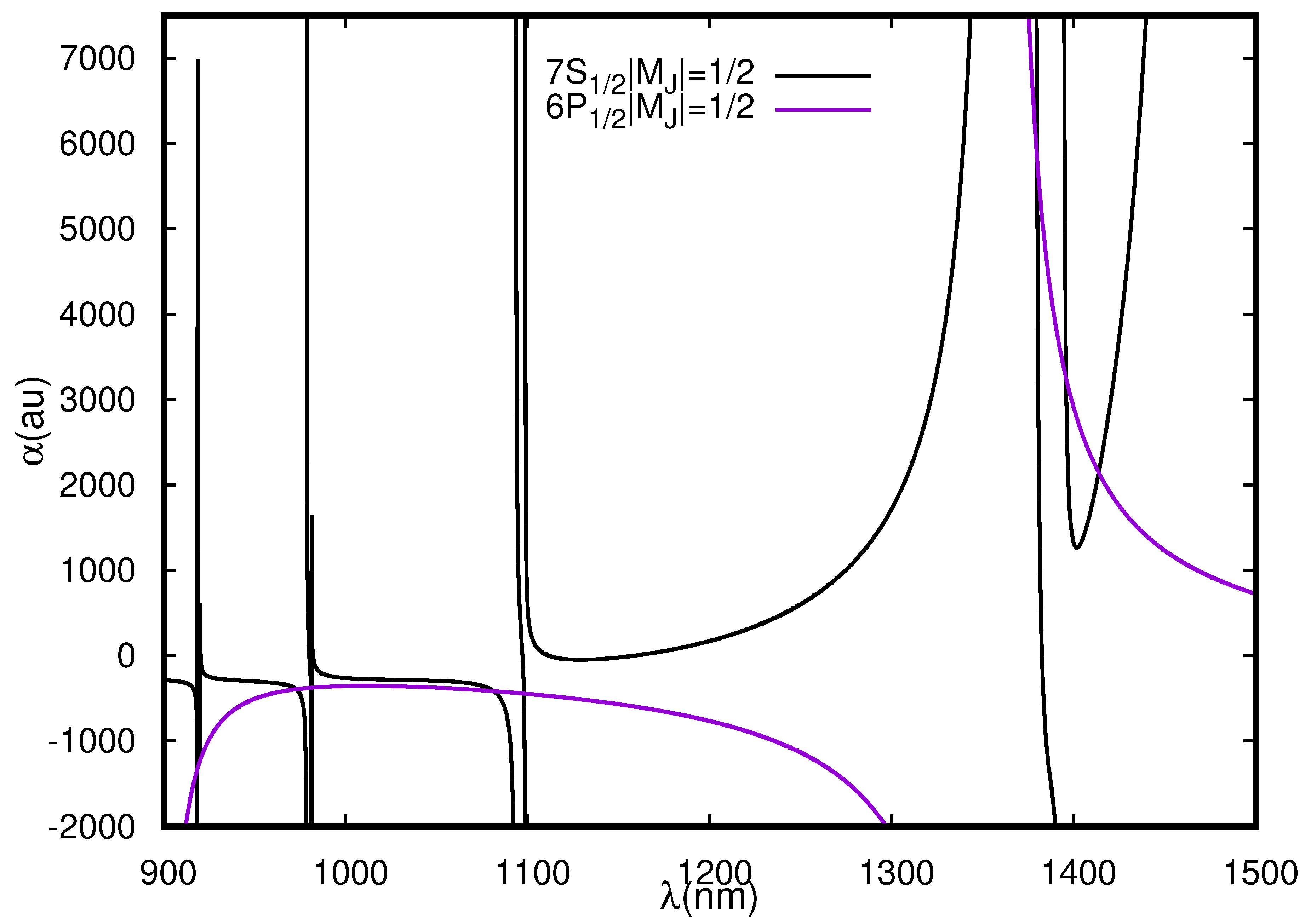
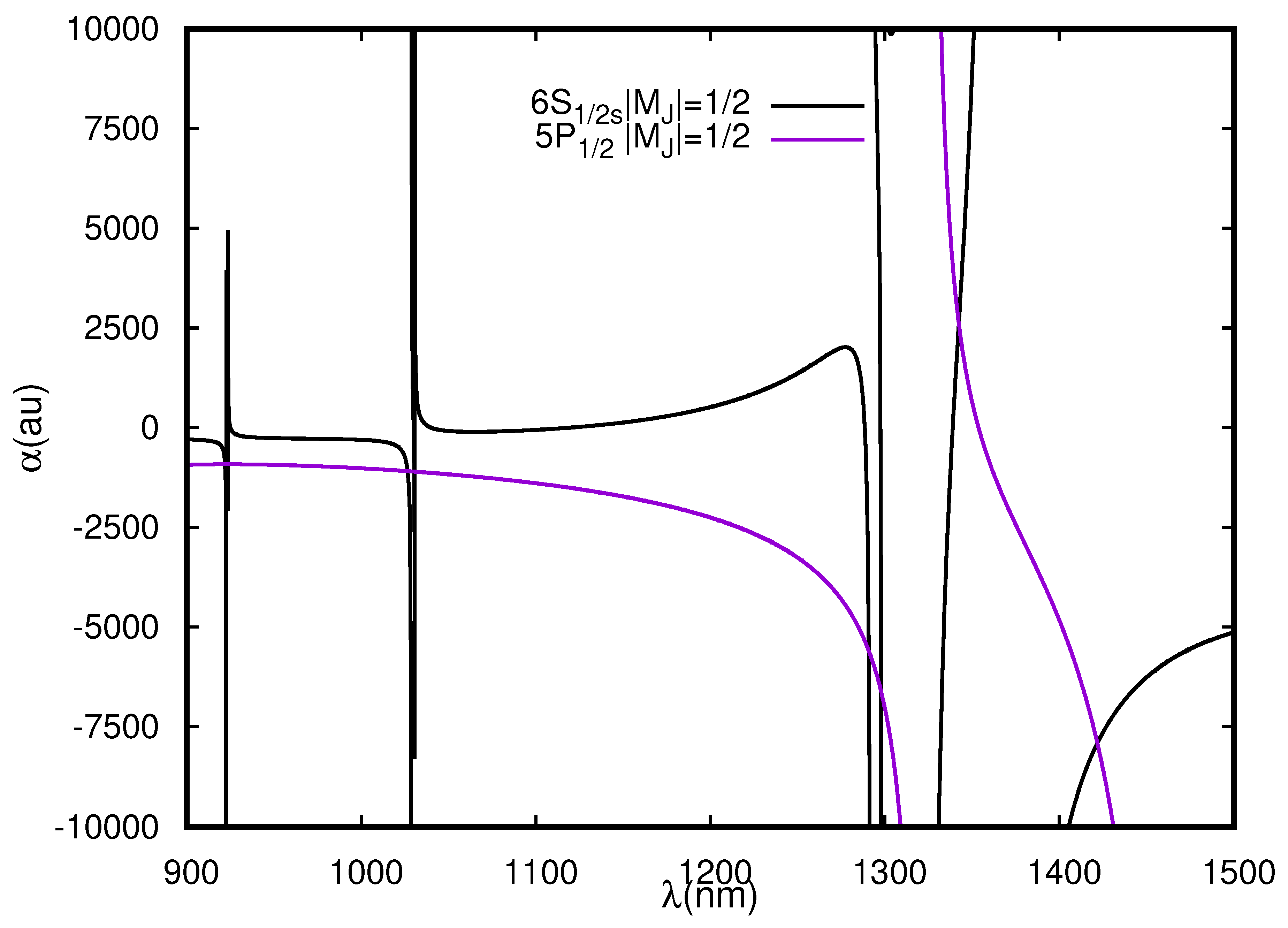
Having evaluated the static dipole polarizability of Cs and Rb atoms, we adopt a similar procedure for calculation of dynamic polarizabilities of these atoms. We anticipate similar accuracies in the dynamic polarizability values as their corresponding static values except at wavelength values in close vicinity of any resonant transition for the considered or states We determine the values of the − and − transitions in Cs () and Rb () atoms using these dynamic polarizabilities. Before we proceed, we would like to clarify that for both (, ) and (, ) levels of the considered transition for Cs and Rb have been calculated. Since for and states, the magic wavelengths among (, ) and (, ) levels for – transition are the same and are shown by the intersection of polarizability curves for and states of Cs and Rb atom in Figure 1 and Figure 2, respectively. To acquire magic wavelength among the (,) levels of the transitions, we plot total dynamic dipolar polarizabilities for the and states for Cs and Rb atoms in Figure 3 and Figure 4, respectively. Similar plots for (, ) levels of transitions are shown in Figure 5 and Figure 6 for Cs and Rb atom, respectively. The results for the (,) and (,) levels are tabulated separately in Table 3 and Table 4 for Cs atom and Table 5 and Table 6 for Rb atom for the ease of pulling out exact values of the magic wavelengths. The resonant wavelengths which are crucial in locating the magic wavelengths are also tabulated.
3.2.1. Cs Atom
As shown in Figure 1 and Table 3, we were able to locate nine s for the transition in Cs within 900–1500 nm. Out of these, six magic wavelengths were located within 900–1100 nm and support blue detuned traps as indicated by negative polarizability values at these wavelengths. The other three located towards higher wavelength range offer red-detuned traps. One would have expected magic wavelengths within 1098–1378 nm where , and resonant transitions occur; however, the opposite nature of and polarizabilities around resonance at 1359 nm prohibits crossing of the and polarizability curves. On the other hand, in Table 3 and Figure 3, we identify seven s for the () transition placed between six different resonances all supporting blue detuned traps. The polarizability of the state has two important resonant transitions ( and ) in the wavelength range considered in this work. In contrast, the polarizability of the state can have significant contributions from several resonant transitions in the considered wavelength range. Thus, they are expected to cross with the polarizability of the states in between these resonant transitions. We find this trend in locating magic wavelengths in between two resonances, except for a few cases where the s are missing. We also find that three s were located between and resonant transitions. Similarly, eight magic wavelengths were found for () transition in the considered wavelength range. It can be noticed from the results in Table 3 that all the magic wavelengths favor red-detuned traps.
We also investigate between the transitions involving the and states. The value of J-dependent polarizability for transition is exactly equal to the F-dependent polarizability value due to the absence of tensor part of the polarizability [49]; hence, we have not tabulated F-dependent values for this transition. The magic wavelengths for the allowed transitions between and states are shown in Figure 5 and listed in Table 4. We choose =0 sublevels in the hyperfine transitions, since, for this particular magnetic sublevel, the first-order Zeeman shift vanishes.
For experimental purposes, it is imperative to choose a magic wavelength which has a low sensitivity towards laser frequency fluctuations and minimum photon scattering. We studied the sensitivity of the magic wavelengths for a 1 nm change in laser wavelength for the and transitions. We noticed that for the transition, magic wavelengths at 973 nm and 1081 nm offer minimum shift in differential stark shifts for a 1 nm change in laser wavelength and are suitable as compared to magic wavelengths at 918.46, 920.101 and 1379.9 nm, which are very sensitive to even a very small change in laser wavelength. The magic wavelengths at 918.46, 920.101 and 1379.9 nm are also very close to the resonance and are expected to have a large photon scattering rate. We recommend the magic wavelength at 1413(2) nm for this transition since it is far detuned and a large value of polarizability value at this wavelength indicates a deep trapping potential. It also offers low sensitivity to laser wavelength fluctuations and small photon scattering rate. For the () transition none of the magic wavelengths support a red-tuned trap. at 1392.4 nm supports a strong blue detuned trap but is very close to the resonances, thus its sensitivity towards the laser fluctuations and photon scattering rate is expected to be very large. On the one hand, the magic wavelength for the () transition at 918.677 supports a very strong red detuned trap but at the same time is extremely sensitive to even small laser wavelength fluctuations. Therefore, we recommend use of at 1213 nm which is far detuned. The recommended magic wavelengths for the F-dependent transitions were investigated in detail by Pan et al. [21] and it was identified that at 1181 nm for the is most suitable for experimental purposes since it offers a strong trapping potential not only for the clock states but also for the other two levels involved in the active clock lasing. Moreover, it was found to provide very low sensitivity against variation in the trapping laser wavelength along with a very low photon scattering rate.
3.2.2. Rb Atom
At least nine s are located for the transition lying systematically between twelve resonant transitions in the considered wavelength range. The magic wavelengths are pictorially presented in Figure 2 and listed in Table 5. Comparing with the results published by Xiao-Run et al. [50], we ascertain that our results are in reasonable agreement with them; however, we have not considered magic wavelengths below 900 nm as we encountered a large number of resonances for the state in this wavelength range. Xiao-Run et al. [50] quoted magic wavelengths at 1342 and 1421 nm for the transition, which agree well with our results at 1342.4(2) and 1421.8(7) nm. According to the evaluations, it is analyzed that Rb favors the formation of blue detuned traps for most of the magic wavelengths except for magic wavelengths near 1342 and 2771 nm for the transition. Similarly, the magic wavelengths for the are shown in Figure 6 and listed in Table 5. The figure and table clearly show that none of the evaluated magic wavelengths lying in the range 900–1500 nm for () and () transitions offer a scope for a red detuned trap; however, while exploring the wavelengths in far infrared region, we found possibility of red detuned traps at 2771 nm for these transitions. In the case of transitions, our results at 1336.5(2) and 1453.3(8) nm match well with the results published in [50]. Similarly in Figure 6 and Table 6, we list the values for all allowed transitions. The F-dependent polarizabilities values at the respective s are listed as well. For this wavelength range, 34 s are located, out of which 30 s support blue detuned traps.
For the transition, s at 1342.4 and 1421.8 nm are recommended for a red-detuned and a blue-detuned trap, respectively. The former wavelength offers less sensitivity to the fluctuations in laser wavelengths as compared to the later magic wavelength. Both these magic wavelengths are far-detuned and will provide very small photon scattering. s at 1461.7 and 1453.3 nm for the () and () transitions, respectively, are recommended for experiments with blue-detuned traps and are least sensitive to the fluctuations in laser wavelengths.
4. Conclusions
We present a list of reliable magic wavelengths for the and transitions for Cs and Rb atoms, respectively, considering the linearly polarized light. These magic wavelengths will be useful for the purpose of trapping of atoms in optical traps for constructing active optical clocks. We calculated static dipolar polarizabilities for the and states of Cs atom, and for the and states of Rb atom. The reliability of these results was verified by comparing the static dipole polarizability values with the other available theoretical and experimental results. The reported electric dipole matrix elements determined for the evaluation of dipole polarizabilities of the above states will be very useful for other studies using the Rb and Cs atoms in the future.
Author Contributions
B.A. conceived the idea of excited state transitions i.e., 7S-6P1/2,3/2 and 6S-5P1/2,3/2 transitions in Cs and Rb atoms respectively for optical-lattice based active clocks proposal. B.A. took the lead of the work and encouraged S.S. and J. to investigate static dipole polarizabilities and magic wavelengths for the considered transitions in Cs and Rb.; S.S. developed the theory and formalism and calculated the results for static dipole polarizabilities for 6S1/2, 5P1/2,3/2 states of Rb and 7S1/2, 6P1/2,3/2 states of Cs. S.S. also evaluated magic wavelengths for the above stated transitions in Rb and Cs, created the tables and designed the figures for the same; J. verified the results for magic wavelengths by independent implementation and contributed in the write-up of manuscript with the support of B.A., J. edited the manuscript and drafted it to the final version by implementing the suggestions of all the authors; B.K.S. and Y.-m.Y. provided critical feedback and helped shape the research, analysis and manuscript, they also aided in interpretation and discussion of the results and commented on the manuscript. All authors have read and agreed to the published version of the manuscript.
Funding
The work of B.A. is supported by DST-SERB(India) Grant No. EMR/2016/001228.
Conflicts of Interest
The authors declare no conflict of interest.
References
- Norcia, M.A.; Winchester, M.N.; Cline, J.R.K.; Thompson, J.K. Superradiance on the millihertz linewidth strontium clock transition. Sci. Adv. 2016, 2, e1601231. [Google Scholar] [CrossRef] [Green Version]
- Chen, J.; Chen, X. Optical lattice laser. In Frequency Control Symposium and Exposition; IEEE: Vancouver, BC, Canada, 2005; p. 3. [Google Scholar]
- Yu, D.; Chen, J. Optical clock with millihertz linewidth based on a phase-matching effect. Phys. Rev. Lett. 2007, 98, 050801. [Google Scholar] [CrossRef]
- Meiser, D.; Ye, J.; Carlson, D.R.; Holland, M.J. Prospects for a millihertz-linewidth laser. Phys. Rev. Lett. 2009, 102, 163601. [Google Scholar] [CrossRef] [PubMed] [Green Version]
- Chen, J. Active optical clock. Chin. Sci. Bull. 2009, 54, 348–352. [Google Scholar]
- Major, F.G. The Quantum Beat: Principles and Applications of Atomic Clocks; Springer: New York, NY, USA, 2015. [Google Scholar]
- Schawlow, A.L.; Devlin, G.E. Intermediate State of Superconductors: Influence of Crystal Structure. Phys. Rev. 1958, 110, 1011. [Google Scholar] [CrossRef]
- Kuppens, S.J.; van Exter, M.P.; Woerdman, J.P. Quantum-limited linewidth of a bad-cavity laser. Phys. Rev. Lett. 1994, 72, 3815. [Google Scholar] [CrossRef]
- Zhang, T.; Wang, Y.; Zang, X.; Zhuang, W.; Chen, J. Active optical clock based on four-level quantum system. Chin. Sci. Bull. 2013, 58, 2033–2038. [Google Scholar] [CrossRef] [Green Version]
- Bohnet, J.G.; Chen, Z.; Weiner, J.M.; Cox, K.C.; Thompson, J.K. Relaxation oscillations, stability, and cavity feedback in a superradiant Raman laser. Phys. Rev. Lett. 2012, 109, 253602. [Google Scholar] [CrossRef] [Green Version]
- Bohnet, J.; Chen, Z.; Weiner, J.; Cox, K.; Thompson, J. Linear-response theory for superradiant lasers. Phys. Rev. A 2014, 89, 013806. [Google Scholar] [CrossRef] [Green Version]
- Christensen, B.T.R.; Henriksen, M.R.; Schaffer, S.A.; Westergaard, P.G.; Ye, J.; Holland, M.; Thomsen, J.W. Non-linear Spectroscopy of Sr Atoms in an Optical Cavity for Laser Stabilization. Phys. Rev. A 2015, 92, 053820. [Google Scholar] [CrossRef] [Green Version]
- Kazakov, G.; Schumm, T. Stability analysis for bad cavity lasers using inhomogeneously boradened spin −1/2 atoms as a gain medium. Phys. Rev. A 2017, 95, 023839. [Google Scholar] [CrossRef] [Green Version]
- Weiner, J.M.; Cox, K.C.; Bohnet, J.G.; Thompson, J.K. Phase synchronization inside a superradiant laser. Phys. Rev. A 2017, 95, 033808. [Google Scholar] [CrossRef] [Green Version]
- Kazakov, G.; Bohnet, J.; Schumm, T. Prospects for a bad-cavity laser using a large ion crystal. Phys. Rev. A 2017, 96, 023412. [Google Scholar] [CrossRef] [Green Version]
- Norcia, M.A.; Thompson, J.K. Cold-Strontium Laser in the Superradiant Crossover Regime. Phys. Rev. X 2016, 6, 011025. [Google Scholar] [CrossRef] [Green Version]
- Norcia, M.A.; Cline, J.R.K.; Muniz, J.A.; Robinson, J.M.; Hutson, R.B.; Goban, A.; Marti, G.E.; Ye, J.; Thompson, J.K. Frequency measurements of superradiance from the strontium clock transition. Phys. Rev. X 2018, 8, 021036. [Google Scholar] [CrossRef] [Green Version]
- Liu, G.; Wang, Y.; Zhang, X.; Yuan, B.; Han, C.; Xue, F. Superradiant Laser with Ultra-Narrow Linewidth Based on 40Ca. Chin. Phys. Lett. 2012, 29, 73202. [Google Scholar]
- Xu, Z.; Zhuang, W.; Wang, Y.; Wang, D.; Zhang, X.; Xue, X.; Pan, D.; Chen, J. Lasing of Cesium four-level active optical clock. In Proceedings of the European Frequency and Time Forum & International Frequency Control Symposium, Prague, Czech Republic, 21–25 July 2013; p. 395. [Google Scholar]
- Pan, D.; Xu, Z.; Xue, X.; Zhuang, W.; Chen, J. Lasing of cesium active optical clock with 459 nm laser pumping. In Proceedings of the Internatinal Frequency Control Symposium, Taipei, Taiwan, 19–22 May 2014; p. 1. [Google Scholar]
- Pan, D.; Arora, B.; mei Yu, Y.; Sahoo, B.K.; Chen, J. Optical-lattice based Cs active clock with continual superradiant lasing signal. arXiv 2020, arXiv:2008.11397. [Google Scholar]
- Katori, H.; Ido, T.; Kuwata-Gonokami, M. Optimal design of dipole potentials for efficient loading of Sr atoms. J. Phys. Soc. Jpn. 1999, 68, 2479–2482. [Google Scholar] [CrossRef]
- Takamoto, M.; Hong, F.L.; Higashi, R.; Katori, H. An optical lattice clock. Nature 2005, 435, 321–324. [Google Scholar] [CrossRef]
- Ovsiannikov, V.D.; Pal’chikov, V.G.; Taichenachev, A.V.; Yudin, V.I.; Katori, H.; Takamoto, M. Magic-wave-induced S 0 1- P 0 3 transition in even isotopes of alkaline-earth-metal-like atoms. Phys. Rev. A 2007, 75, 020501. [Google Scholar] [CrossRef]
- Arora, B.; Safronova, M.S.; Clark, C.W. Magic wavelengths for the np–ns transitions in alkali-metal atoms. Phys. Rev. A 2007, 76, 052509. [Google Scholar] [CrossRef] [Green Version]
- Singh, S.; Kaur, K.; Sahoo, B.K.; Arora, B. Comparing magic wavelengths for the 6s2S1/2-6p2P1/2,3/2 transitions of Cs using circularly and linearly polarized light. J. Phys. B At. Mol. Opt. Phys. 2016, 49, 145005. [Google Scholar] [CrossRef] [Green Version]
- Kaur, J.; Nandy, D.K.; Arora, B.; Sahoo, B.K. Properties of alkali-metal atoms and alkaline-earth-metal ions for an accurate estimate of their long-range interactions. Phys. Rev. A 2015, 91, 1012705. [Google Scholar] [CrossRef]
- Schäffer, S.A.; Christensen, B.T.R.; Rathmann, S.M.; Appel, M.H.; Henriksen, M.R.; Thomsen, J.W. Towards passive and active laser stabilization using cavity-enhanced atomic interaction. In Proceedings of the International Conference on Spectral Line Shapes, Torun, Poland, 19–24 June 2016. [Google Scholar]
- Topcu, T.; Derevianko, A. Possibility of triple magic trapping of clock and Rydberg states of divalent atoms in optical lattices. J. Phys. B At. Mol. Opt. Phys. 2016, 49, 144004. [Google Scholar] [CrossRef] [Green Version]
- Iskrenova-Tchoukova, E.; Safronova, M.S.; Safronova, U.I. High-precision study of Cs polarizabilities. J. Comp. Meth. Sci. Eng. 2007, 7, 521. [Google Scholar] [CrossRef]
- Bonin, K.D.; Kresin, V.V. Electric-Dipole Polarizabilities of Atoms, Molecules and Clusters; World Scientific: Singapore, 1997. [Google Scholar]
- Manakov, N.L.; Ovsiannikov, V.D.; Rapoport, L.P. Atoms in a laser field. Phys. Rep. 1986, 141, 319. [Google Scholar] [CrossRef]
- Singh, S.; Sahoo, B.K.; Arora, B. Magnetic-sublevel-independent magic wavelengths: Application to Rb and Cs atoms. Phys. Rev. A 2016, 93, 063422. [Google Scholar] [CrossRef] [Green Version]
- Blundell, S.A.; Johnson, W.R. Sapirstein J Relativistic all-order calculations of energies and matrix elements in cesium. Phys. Rev. A 1991, 43, 3407. [Google Scholar] [CrossRef]
- Johnson, W.R.; Idrees, M. Sapirstein, J Second-order energies and third-order matrix elements of alkali-metal atoms. Phys. Rev. A 1987, 35, 8. [Google Scholar] [CrossRef]
- Blundell, S.; Johnson, W.; Liu, Z.; Sapirstein, J. Relativistic all-order calculations of energies and matrix elements for Li and Be+. Phys. Rev A 1989, 40, 2233. [Google Scholar] [CrossRef]
- Safronova, M.S.; Johnson, W.R. All-Order Methods for Relativistic Atomic Structure Calculations. Adv. At. Mol. Opt. Phys. 2007, 55, 191. [Google Scholar]
- Safronova, M.S. High-Precision Calculation of Atomic Properties and Parity Nonconservation in Systems with One Valence Electron. Ph.D. Thesis, University of Notre Dame, Notre Dame, IN, USA, 2001. [Google Scholar]
- Kramida, A.; Ralchenko, Y.; Reader, J. NIST Atomic Spectra Database; Version 5; National Institute of Standards and Technology: Gaithersburg, MD, USA, 2012. Available online: http://physics.nist.gov/asd (accessed on 12 December 2012).
- van Wijngaarden, W.; Li, J. Polarizabilities of cesium S, P, D, and F states. Quant. Spectrosc. Radiat. Transf. 1994, 52, 555. [Google Scholar] [CrossRef]
- Bates, D.R.; Damgaard, A. The calculation of the absolute strengths of spectral lines. Philos. Trans. R. Soc. 1949, 242, 101. [Google Scholar]
- Hunter, L.R.; Krause, D.; Miller, K.E.; Berkeland, D.J.; Boshier, M.G. Precise measurement of the Stark shift of the cesium D1 line. Opt. Commun. 1992, 94, 210. [Google Scholar] [CrossRef]
- Tanner, C.E.; Wieman, C.E. Precision measurement of the Stark shift in the 6P1/2–6P2/3 cesium transition using a frequency-stabilized laser diode. Phys. Rev. A 1988, 38, 162. [Google Scholar] [CrossRef]
- van Wijngaarden, W. Scalar and tensor polarizabilities of low lying S, P, D, F and G states in rubidium. J. Quant. Spectrosc. Radiat. Transf. 1997, 57, 275. [Google Scholar] [CrossRef]
- Zhu, C.; Dalgarno, A.; Porsev, S.G.; Derevianko, A. Dipole polarizabilities of excited alkali-metal atoms and long-range interactions of ground- And excited-state alkali-metal atoms with helium atoms. Phys. D At. Mol. Clust. 1997, 41, 229. [Google Scholar] [CrossRef] [Green Version]
- Miller, K.E.; Krause, D.; Hunter, L.R. Precise measurement of the Stark shift of the rubidium and potassium D1 lines. Phys. Rev. A 1994, 49, 5128. [Google Scholar] [CrossRef]
- Krenn, C.; Scherf, W.; Khaitm, O.; Musso, M.; Windholz, L. Stark effect investigations of resonance lines of neutral potassium, rubidium, europium and gallium Z. Phys. D At. Mol. Clust. 1997, 41, 229–233. [Google Scholar] [CrossRef]
- Bennett, S.C.; Roberts, J.L.; Wieman, C.E. Measurement of the dc Stark shift of the 6S→7S transition in atomic cesium. Phys. Rev. A 1999, 59, 16(R). [Google Scholar] [CrossRef]
- Kaur, J.; Singh, S.; Arora, B.; Sahoo, B.K. Annexing magic and tune-out wavelengths to the clock transitions of the alkaline-earth-metal ions. Phys. Rev. A 2017, 95, 042501. [Google Scholar] [CrossRef] [Green Version]
- Xiao, Z.; Tong, Z.; Jing, C. Magic wavelengths for a lattice trapped rubidium four-level active optical clock. Chin. Phys. Lett. 2012, 29, 090601. [Google Scholar]
Figure 1.
Dynamic polarizabilities (in a.u.) of and states of Cs in the wavelength range 900–1500 nm for linearly polarized light.
Figure 1.
Dynamic polarizabilities (in a.u.) of and states of Cs in the wavelength range 900–1500 nm for linearly polarized light.

Figure 2.
Dynamic polarizabilities (in a.u.) of the and states of Rb in the wavelength range 900–1500 nm for the linearly polarized light.
Figure 2.
Dynamic polarizabilities (in a.u.) of the and states of Rb in the wavelength range 900–1500 nm for the linearly polarized light.

Figure 3.
J-dependent dynamic polarizabilities (in a.u.) of the and states of Cs in the wavelength range 900–1500 nm for linearly polarized light.
Figure 3.
J-dependent dynamic polarizabilities (in a.u.) of the and states of Cs in the wavelength range 900–1500 nm for linearly polarized light.

Figure 4.
J-dependent dynamic polarizabilities (in a.u.) of the and states of Rb in the wavelength range 900–1500 nm for linearly polarized light.
Figure 4.
J-dependent dynamic polarizabilities (in a.u.) of the and states of Rb in the wavelength range 900–1500 nm for linearly polarized light.

Figure 5.
F-dependent dynamic polarizabilities (in a.u.) of the and states of Cs in the wavelength range 900–1500 nm for linearly polarized light.
Figure 5.
F-dependent dynamic polarizabilities (in a.u.) of the and states of Cs in the wavelength range 900–1500 nm for linearly polarized light.

Figure 6.
F-dependent dynamic polarizabilities (in a.u.) of the and states of Rb in the wavelength range 900–1500 nm for linearly polarized light.
Figure 6.
F-dependent dynamic polarizabilities (in a.u.) of the and states of Rb in the wavelength range 900–1500 nm for linearly polarized light.


Table 1.
Contributions from different E1 matrix elements (d) to the static polarizabilities (in a.u.) of the , and states of Cs atom. The final results are compared with the previously estimated and available experimental results. Uncertainties are given in the parentheses.
Table 1.
Contributions from different E1 matrix elements (d) to the static polarizabilities (in a.u.) of the , and states of Cs atom. The final results are compared with the previously estimated and available experimental results. Uncertainties are given in the parentheses.
| State | State | State | |||||||
|---|---|---|---|---|---|---|---|---|---|
| Transition | Transition | Transition | |||||||
| 4.25(9) | −179(8) | 4.489(7) | −131.9(4) | 6.324(7) | −124.7(3) | 124.7(3) | |||
| 10.33(5) | 2415(23) | 4.25(9) | 180(8) | 6.49(8) | 226(5) | −226(5) | |||
| 0.929(9) | 8.8(2) | 1.0(1) | 6(1) | 1.5(1) | 6(1) | −6(1) | |||
| 0.356(7) | 1.02(4) | 0.55(6) | 1.4(3) | 0.77(8) | 1.4(3) | −1.4(3) | |||
| 0.185(5) | 0.25(1) | 0.36(4) | 0.57(9) | 0.51(5) | 0.6(1) | −0.6(1) | |||
| 6.49(8) | −453(11) | 7.02(2) | 1084(7) | 3.17(2) | 133(1) | 106(1) | |||
| 14.34(5) | 4413(31) | 4.3(4) | 121(2) | 2.1(2) | 15(3) | 12(3) | |||
| 1.64(1) | 27.3(5) | 2.1(2) | 21(4) | 1.0(1) | 2.5(5) | 2.0(4) | |||
| 0.70(1) | 3.9(1) | 1.3(1) | 7(1) | 0.61(6) | 0.8(2) | 0.7(1) | |||
| 0.388(8) | 1.08(4) | 0.93(9) | 3.6(7) | 0.43(4) | 0.40(8) | 0.32(6) | |||
| 0.71(7) | 2.0(4) | 0.33(3) | 0.22(4) | 0.18(4) | |||||
| 9.59(8) | 1174(20) | −235(4) | |||||||
| 6.3(6) | 132(26) | −26(5) | |||||||
| 2.9(3) | 22(4) | −4.3(9) | |||||||
| 1.8(2) | 7(1) | −1.5(3) | |||||||
| 1.3(1) | 3.5(7) | −0.7(1) | |||||||
| 1.0(1) | 2.0(4) | −0.40(8) | |||||||
| Main() | 6238(41) | Main() | 1295(12) | Main() | 1602(33) | −256(9) | |||
| Tail() | 4(2) | Tail() | 28(14) | Tail() | 30(9) | −6(2) | |||
| −0.47 | ∼0 | ∼0 | ∼0 | ||||||
| 15.8(3) | 15.8(3) | 15.8(3) | |||||||
| Total | 6257(41) | Total | 1339(18) | Total | 1648(35) | −262(9) | |||
| Others | 6238(41) [30] | Others | 1338 [25] | Others | 1650 [25] | −261 [25] | |||
| 6140 [40] | 1290 [40] | 1600 [40] | −233 [40] | ||||||
| Experiment | 6238(6) [48] | Experiment | 1328.4(6) [42] | Experiment | 1641(2) [43] | −262(2) [43] | |||
Table 2.
Contributions from different E1 matrix elements (d) to the static polarizabilities (in a.u.) of the , and states of Rb atom. The final results are compared with the previously estimated and available experimental results. Uncertainties are given in the parentheses.
Table 2.
Contributions from different E1 matrix elements (d) to the static polarizabilities (in a.u.) of the , and states of Rb atom. The final results are compared with the previously estimated and available experimental results. Uncertainties are given in the parentheses.
| State | State | State | |||||||
|---|---|---|---|---|---|---|---|---|---|
| Transition | Transition | Transition | |||||||
| 4.15(3) | −167(2) | 4.231(3) | −104.1(1) | 5.977(4) | −102.0(1) | 102.0(1) | |||
| 9.68(6) | 1915(24) | 4.15(3) | 167(2) | 6.05(3) | 183(2) | −183(2) | |||
| 0.999(6) | 9.5(1) | 0.953(2) | 4.83(1) | 1.350(2) | 4.94(2) | −4.94(2) | |||
| 0.393(4) | 1.2(2) | 0.502(2) | 1.120(7) | 0.708(2) | 1.129(7) | −1.129(7) | |||
| 6.05(3) | −366(4) | 8.05(7) | 700(12) | 3.63(3) | 74(1) | 59(1) | |||
| 13.6(1) | 3693(54) | 1.35(6) | 10(1) | 0.66(3) | 1.3(1) | 1.01(9) | |||
| 1.54(1) | 22.4(3) | 1.1(1) | 5(1) | 0.51(5) | 0.6(1) | 0.5(1) | |||
| 0.628(7) | 2.967(7) | 0.79(6) | 2.6(4) | 0.37(3) | 0.29(4) | 0.23(3) | |||
| 0.61(4) | 1.4(2) | 0.28(2) | 0.16(2) | 0.13(2) | |||||
| 10.90(9) | 665(11) | −133(2) | |||||||
| 1.98(9) | 11(1) | −2.2(2) | |||||||
| 1.5(1) | 5(1) | −1.1(2) | |||||||
| 1.10(8) | 2.5(4) | −0.51(7) | |||||||
| 0.8(5) | 1.4(2) | −0.28(3) | |||||||
| Main() | 5112(59) | Main() | 788(12) | Main() | 849(11) | −163(2) | |||
| Tail() | 3(2) | Tail() | 16(8) | Tail() | 17(9) | −5(3) | |||
| −0.26 | ∼0 | ∼0 | ∼0 | ||||||
| 9.08(45) | 9.08(45) | 9.08(45) | |||||||
| Total | 5124(59) | Total | 813(14) | Total | 875(14) | −168(4) | |||
| Others | 5110 [44] | Others | 805 [25] | Others | 867 [25] | −167 [25] | |||
| 807 [45] | 870 [45] | −171 [45] | |||||||
| Experiment | 810.6(6) [46] | Experiment | 857(10) [47] | −163(3) [47] | |||||
Table 3.
Magic wavelengths (s) (in nm) with corresponding polarizabilities (s) (in a. u.) for the and transitions in the Cs atom with the linearly polarized lights along with the resonant wavelengths (s) (in nm).
Table 3.
Magic wavelengths (s) (in nm) with corresponding polarizabilities (s) (in a. u.) for the and transitions in the Cs atom with the linearly polarized lights along with the resonant wavelengths (s) (in nm).
| Resonance | Resonance | |||||||||
|---|---|---|---|---|---|---|---|---|---|---|
| 894.59 | 917.48 | |||||||||
| 918.46(2) | −1335 | |||||||||
| 918.671 | 918.671 | |||||||||
| 920.101(4) | −1225 | 918.677(3) | 35,277 | |||||||
| 920.141 | 920.141 | |||||||||
| 973(3) | −393 | 921.0(9) | −147 | 920.3(3) | 56 | |||||
| 978.651 | 921.11 | |||||||||
| 980.86(5) | −376 | 978.651 | ||||||||
| 981.231 | 980.1(7) | −14 | 979.01(8) | 1126 | ||||||
| 1081(5) | −415 | 981.231 | ||||||||
| 1093.356 | 982(2) | −46 | 981.33(3) | 1088 | ||||||
| 1097.92(6) | −444 | 1005(5) | −269 | |||||||
| 1098.723 | 1088(3) | −625 | ||||||||
| 1359.201 | 1093.356 | |||||||||
| 1378.173 | 1098.09(9) | −661 | 1095.9(3) | 424 | ||||||
| 1379.9(1) | 5830 | 1098.723 | ||||||||
| 1394.057 | 1100.6(8) | 413 | ||||||||
| 1395.8(2) | 3248 | 1213(6) | 249 | |||||||
| 1413(2) | 2145 | 1359.201 | ||||||||
| 1469.892 | 1378.173 | |||||||||
| 1392.4(1) | −4207 | 1382.4(5) | 113 | |||||||
| 1394.057 | ||||||||||
| 1469.892 | ||||||||||
Table 4.
s (in nm) and their corresponding polarizabilities (in a.u.) in Cs (I = 7/2) of the transitional states involved in transition are listed.
Table 4.
s (in nm) and their corresponding polarizabilities (in a.u.) in Cs (I = 7/2) of the transitional states involved in transition are listed.
| 920.8(1) | −119 | 920.5(3) | −35 |
| 979.3(3) | 398 | 979.1(1) | 938 |
| 981.5(2) | 366 | 981.35(4) | 901 |
| 1097.7(2) | −274 | 1096.5(4) | 243 |
| 1102(3) | 229 | ||
| 1181(8) | 73 | ||
| 1391.2(5) | −2623 | 1383.5(9) | −533 |
| 920.6(1) | −81 | 920.9(1) | −136 |
| 979.1(1) | 722 | 979.6(6) | 180 |
| 981.38(7) | 687 | 982(1) | 150 |
| 1043(9) | −290 | ||
| 1082(3) | −430 | ||
| 1097.1(4) | 36 | 1097.9(1) | −480 |
| 1112(5) | −1 | ||
| 1130(7) | −47 | ||
| 1386(2) | −1320 | 1392.0(2) | −3469 |
Table 5.
Magic wavelengths (s) (in nm) with corresponding polarizabilities (s) (in a. u.) for the transition in the Rb atom with the linearly polarized lights along with the resonant wavelengths (s) (in nm).
Table 5.
Magic wavelengths (s) (in nm) with corresponding polarizabilities (s) (in a. u.) for the transition in the Rb atom with the linearly polarized lights along with the resonant wavelengths (s) (in nm).
| Resonance | Resonance | ||||||||
|---|---|---|---|---|---|---|---|---|---|
| 867.95 | 867.95 | ||||||||
| 921.96(2) | −917 | 922.281(9) | −1351 | ||||||
| 922.71 | 922.71 | ||||||||
| 923.533(3) | −917 | 923.569(2) | −1350 | 923.414(6) | −301 | ||||
| 923.67 | 923.67 | ||||||||
| 1026.58(9) | −1090 | 1027.31(5) | −1516 | 1020.6(6) | −467 | ||||
| 1028.67 | 1028.67 | ||||||||
| 1030.336(9) | −1102 | 1030.395(7) | −1526 | 1030.20(1) | −487 | ||||
| 1030.67 | 1030.67 | ||||||||
| 1290.85(3) | −5597 | 1290.80(3) | −5259 | 1289.70(7) | −1583 | ||||
| 1292.28 | 1292.28 | ||||||||
| 1297.867(7) | −6606 | 1297.841(7) | −5671 | 1297.67(1) | −1655 | ||||
| 1298.28 | 1298.28 | ||||||||
| 1323.88 | 1323.88 | ||||||||
| 1342.4(2) | 2609 | 1331.2(1) | −9501 | 1336.5(2) | −2095 | ||||
| 1366.87 | 1366.87 | ||||||||
| 1421.8(7) | −7909 | 1461.7(7) | −5872 | 1453.3(8) | −6139 | ||||
| 1475.65 | 1529.26 | ||||||||
| 2732.18 | 1529.37 | ||||||||
| 2771.1(3) | 1132 | 2732.18 | |||||||
| 2791.29 | 2771.0(3) | 1501 | 2771.1(3) | 1000 | |||||
| 2791.29 | |||||||||
Table 6.
s (in nm) and their corresponding polarizabilities (in a.u.) in Rb (I = 5/2) of transitional states involved in 6S transition are listed.
Table 6.
s (in nm) and their corresponding polarizabilities (in a.u.) in Rb (I = 5/2) of transitional states involved in 6S transition are listed.
| 921.98(2) | −930 | 919.6(4) | −446 |
| 923.534(3) | −930 | 923.455(5) | −451 |
| 1026.60(8) | −1100 | 1023.9(3) | −621 |
| 1030.337(9) | −1110 | 1030.24(1) | −635 |
| 1290.49(4) | -3781 | 1289.94(6) | −2103 |
| 1297.786(8) | −4063 | 1297.71(1) | −2228 |
| 1332.7(1) | −6714 | 1335.3(2) | −3279 |
| 1459.1(9) | −5950 | 1455(1) | −6082 |
| 2771.1(3) | 1300 | 2771.1(3) | 1071 |
| 923.507(3) | −720 | 923.559(2) | −1201 |
| 1025.9(1) | −891 | 1027.12(5) | −1367 |
| 1030.30(1) | −902 | 1030.377(9) | −1377 |
| 1290.28(4) | −3045 | 1290.70(3) | -4731 |
| 1297.753(9) | −3259 | 1297.823(7) | −5097 |
| 1333.7(2) | −5258 | 1331.7(1) | −8520 |
| 1457.5(6) | −6000 | 1460.9(9) | −5897 |
| 2771.1(3) | 1201 | 2771.0(3) | 1429 |
Publisher’s Note: MDPI stays neutral with regard to jurisdictional claims in published maps and institutional affiliations. |
© 2020 by the authors. Licensee MDPI, Basel, Switzerland. This article is an open access article distributed under the terms and conditions of the Creative Commons Attribution (CC BY) license (http://creativecommons.org/licenses/by/4.0/).
Share and Cite
MDPI and ACS Style
Singh, S.; Jyoti; Arora, B.; Sahoo, B.K.; Yu, Y.-m. Magic Wavelengths for Optical-Lattice Based Cs and Rb Active Clocks. Atoms 2020, 8, 79. https://0-doi-org.brum.beds.ac.uk/10.3390/atoms8040079
AMA Style
Singh S, Jyoti, Arora B, Sahoo BK, Yu Y-m. Magic Wavelengths for Optical-Lattice Based Cs and Rb Active Clocks. Atoms. 2020; 8(4):79. https://0-doi-org.brum.beds.ac.uk/10.3390/atoms8040079
Chicago/Turabian StyleSingh, Sukhjit, Jyoti, Bindiya Arora, B. K. Sahoo, and Yan-mei Yu. 2020. "Magic Wavelengths for Optical-Lattice Based Cs and Rb Active Clocks" Atoms 8, no. 4: 79. https://0-doi-org.brum.beds.ac.uk/10.3390/atoms8040079
Note that from the first issue of 2016, this journal uses article numbers instead of page numbers. See further details here.