Bus Service Level and Horizontal Equity Analysis in the Context of the Modifiable Areal Unit Problem

Abstract

The modifiable areal unit problem is of great importance in geographic science. The use of a specific zoning impacts the social and economic imbalances that can be generated in the deployment of services, facilities, and infrastructure. In this article, GIS is used together with simulation and optimization tools to analyse the effects of bus frequency changes in the levels of service and horizontal equity derived from different types of territorial zoning. The city of Palma (Balearic Islands, Spain) was chosen as a case study for the method, for which different geographical areas are used: neighbourhoods, census sections, cadastral blocks, and a 400 × 400 m mesh. The results show significant variations of the optimal frequencies obtained, depending on the type of zoning used. In general, smaller zonings show much higher sensitivity for the detection of imbalances between the population and bus service level. Likewise, orthogonal zonings also prove useful for identifying service and population concentration over other zonings. The use of large spatial units could lead to the misdiagnosis of needs and the implementation of actions that do not actually improve the level of service or the equity of the transport service. It is recommended to consider combining zonings of different sizes simultaneously, in order to accurately highlight imbalances and to argue for transport service improvements.

1. Introduction

The modifiable areal unit problem (MAUP) is a recurrent theme in studies of the geography of services, which still arouses much debate [1,2,3]. In transport planning, many authors have analysed the MAUP in various fields of study, such as bus transport, bicycle transport, and so on [4,5,6,7,8,9].

Public transport planning aims to provide an appropriate level of service to the population while not creating imbalances between territories and social groups [10]. In the diagnostic phases of transport planning studies, it is usual to divide the region into geographical units (e.g., municipalities, neighbourhoods, districts, sections, and so on) and to analyse demand, supply, or equity indicators based on these divisions. However, there has been little debate about the reliability or bias of these data, concerning the type of geographical zoning used.

One of the main factors conditioning the use of a particular spatial unit in transport planning is socio-economic information availability [2]. In fact, it is not always easy to obtain updated spatial information on the social, demographic, or environmental indicators of a territory. For this reason, when these data are available for a specific type of spatial unit, they are usually retained to analyse the needs for services, facilities, or infrastructure. This practice can lead to the generation or hiding of imbalances.

In the framework of service planning, a minimal change in a geographical unit—for example, due to the integration of a block of buildings with residential use—can modify demand levels. A larger population indicates a more significant potential demand for services, which could justify higher economic investments and guide the deployment of assets in one area or another.

The geographical units used in planning may diverge, regarding sizes or surfaces, as well as regarding geometric shapes. Social, economic, historical, cultural, and environmental issues are involved in the delimitation of neighbourhoods. Sometimes, there may be no specific reason why one district is smaller than another or why one may have a larger population than another. In this context, the choice of one or another zoning can be critical.

Planning tasks should include the use of adequate methodological tools to address the population’s needs and to prevent imbalances in the allocation of resources or the supply of services as much as possible. Therefore, it is essential to know what effects the choice of one or other spatial reference units might have.

Bus fleet frequency management is a common practice for matching supply with service levels and demand [11]. The increase or reduction of the frequency of a line can lead to significant changes in the service level of the areas it covers. In this regard, bus stops provide a level of service to the population in an area of influence usually smaller than 400 m [12,13]. Such an area of influence may include part or all of the geographical units into which the territory is divided for demographic, electoral, or planning (zoning) purposes. Therefore, each geographical unit obtains a level of service derived from the bus stops located within or nearby.

Geographic Information Systems (GIS) have experienced continuous functional development since their origin. However, it has sometimes been criticized that their analytical capabilities have not developed as profoundly as their functionalities for capturing, storing, managing, or representing spatial information. The integration of optimization techniques into GIS has not been a very prolific field in the scientific literature, although there have been relevant contributions in transport planning, land-use assignment, waste management, and so on [14,15,16,17,18,19].

As commercial GIS products have few integrated functionalities, in terms of simulation or optimization, the development of integrated optimization applications or the coordinated use of specific programs is joint. During recent years, access to open data sources that contain information on city transportation networks (General Transit Feed Specification GTFS) has enabled the implementation of applications aimed at simulation and optimization [20,21,22]. Using GIS, it is possible to georeference bus lines and stops, calculate areas of influence and zoning, and calculate territorial indicators.

In this study, we examine the application of simulation and optimization techniques in depth, in order to evaluate the effects of changing bus frequencies on the service level of a territory and the consequences derived from the use of different zonings in the calculation of service and equity indicators.

The article is structured as follows: Firstly, an analysis of the state-of-the-art in the scientific literature of transport planning and modifiable spatial units is presented. Secondly, the methodology of the study, based on the integration of GIS with a modelling and simulation system for the analysis of the level of service and equity is presented; then, the main results obtained in the study and their discussion are presented. Finally, the article ends by giving a set of conclusions.

2. Literature Review

It has been established that the practice of public transport planning has changed from a strictly dotational approach to a more preventive approach [23,24], in which priority is given to equity and, especially, to the provision of services for vulnerable groups. From such a perspective, it is very important to have methodologies for evaluating the impact of transport policies on territories that integrate ethical and social justice considerations, in order to determine the equitable distribution of transport services among the population and to comply with minimum standards. However, some authors have pointed out that there is a lack of methodological guidance on how to define and evaluate equity in the supply of transportation services [25].

A difference has been drawn between horizontal equity, which considers that all individuals should receive the same level of service, and vertical equity, which is especially interested in the appropriate provision to disadvantaged groups [26,27,28]. Therefore, horizontal equity is focused more on aspects relating to the equitable territorial distribution of the service, in which land-use and the distribution of the population play fundamental roles, while vertical equity is of a social nature, in which the access to transport by socially excluded groups is more important [29].

On such a conceptual basis, the scientific literature unfolds along several thematic lines relevant to this research:

Accessibility and equity—Lucas et al. [30] proposed prioritizing accessibility over mobility to balance the deployment of services and infrastructures.

Equity and cost of travel—El-Geneidy, A. et al. [31] investigated in the cost of equity in transport by assessing the differences in travel costs in a territory.

Socio-economic activities and public transport—Liu and Duan [32] identified a close relationship between the design of urban bus routes and the intensity of socio-economic activities; while Chahar and Smith-Colin [33] identified “transit deserts”, areas with a unique lack of facilities, based on integrated accessibility indicators.

Access to public transport and employment—Cebollada et al. [34] studied the relationship between employment and access to public transport; while Barboza et al. [35] analysed the inequity of accessibility, considering 160 neighbourhoods in Rio de Janeiro, to areas that generate employment and proposed calculating the “Balancing Time” indicator.

Equity in access to emerging sustainable transport services—Guo et al. [36] analysed how access to electric vehicles and shared mobility can lead to significant social and territorial imbalances; while Mooney et al. [37] and Braun et al. [38] analysed spatial imbalances concerning access to public bicycle systems.

Methodologies of equity analysis in transport—Sharma et al. [39] proposed an equity analysis methodology to be used in public transport agencies based on the evaluation of traffic connectivity using open-source data sets; Manrique et al. [40] proposed a method for analysing the overall equity of a transport system based on the resident population’s level of transport needs; Romero et al. [41] proposed a method for optimizing the transport of dangerous goods and equipment, based on horizontal equity analysis by calculating the Gini coefficient; and Park and Chang [42] used GIS techniques and calculation of the Gini coefficient to evaluate the spatial equity of access to the transport service in Seoul.

The path towards sustainable mobility requires taking a further step in understanding the territory, in order to minimize travel costs and adjust them to demand, and developing innovative quality schemes that gain the trust and acceptance of people [43].

It has been noted that there is a lack of scientific literature on the analysis of the effects of zoning/geographical scale on the bus service level and equity, in spite of the relevance of the subject. Horner and Murray showed that the aggregation and definition of spatial units can greatly impact the estimation of excess displacement [44]. Kwan and Weber, focusing on accessibility and its relationship with land-uses, concluded that multi-scale relationships remain invariant to scale changes [45]. The effects of scale and zoning in the analysis of school transport have been analysed by Mitra and Buliung [5], indicating that studies that use a single geographical representation can produce misleading results and, therefore, advising that the units selected should always take into account the interaction of behaviour and the surrounding physical environment. Xu et al. [46] revealed that, when the size of spatial units decreases and their number increases, significant groupings are not noticeable on other scales. Pani et al. [47] showed that a planner in freight transport can obtain different indicators, depending on how the data are aggregated, referring to land-use and transport infrastructure.

It has been shown that the choice of territorial zoning can have a direct influence on the calculation of service levels and accessibility and have a singular transcendence in the planning of transport infrastructure and services. Several components of territorial accessibility may be significantly affected by the choice of one or another zoning. We consider that it is essential to have a thorough knowledge of this problem. In this sense, Neutens [48] emphasized the need to improve further spatial aggregation and the analytical methods developed to analyse transport equity further.

Based on the scientific literature reviewed, it can be noted that there has been no in-depth analysis of the effect of the MAUP on the diagnosis of the level of bus transport service and its equity. In the various studies carried out, different zoning systems have been used by default; however, the effects of a change of zoning system were not analysed. In this article, we formulate the following hypotheses: the diagnosis of the bus service and its equity should provide very similar results regardless of the zoning used; the increase of frequencies in bus lines will always produce improvements in the level of service of the transport system and in its equity, as it means improving the access times.

To test these hypotheses, the following tasks were carried out: First, the geographical distribution of the level of service and equity in different zonings is evaluated, through use of a methodology that integrates GIS tools and mathematical analysis. Secondly, a simulation process of the level of service and equity is developed, from bus frequency modelling, which analyses the sensibility of bus lines to each zoning. Finally, an optimization model of bus line frequencies is proposed, in order to maximize the level of service and equity in each type of zoning.

3. Materials and Methods

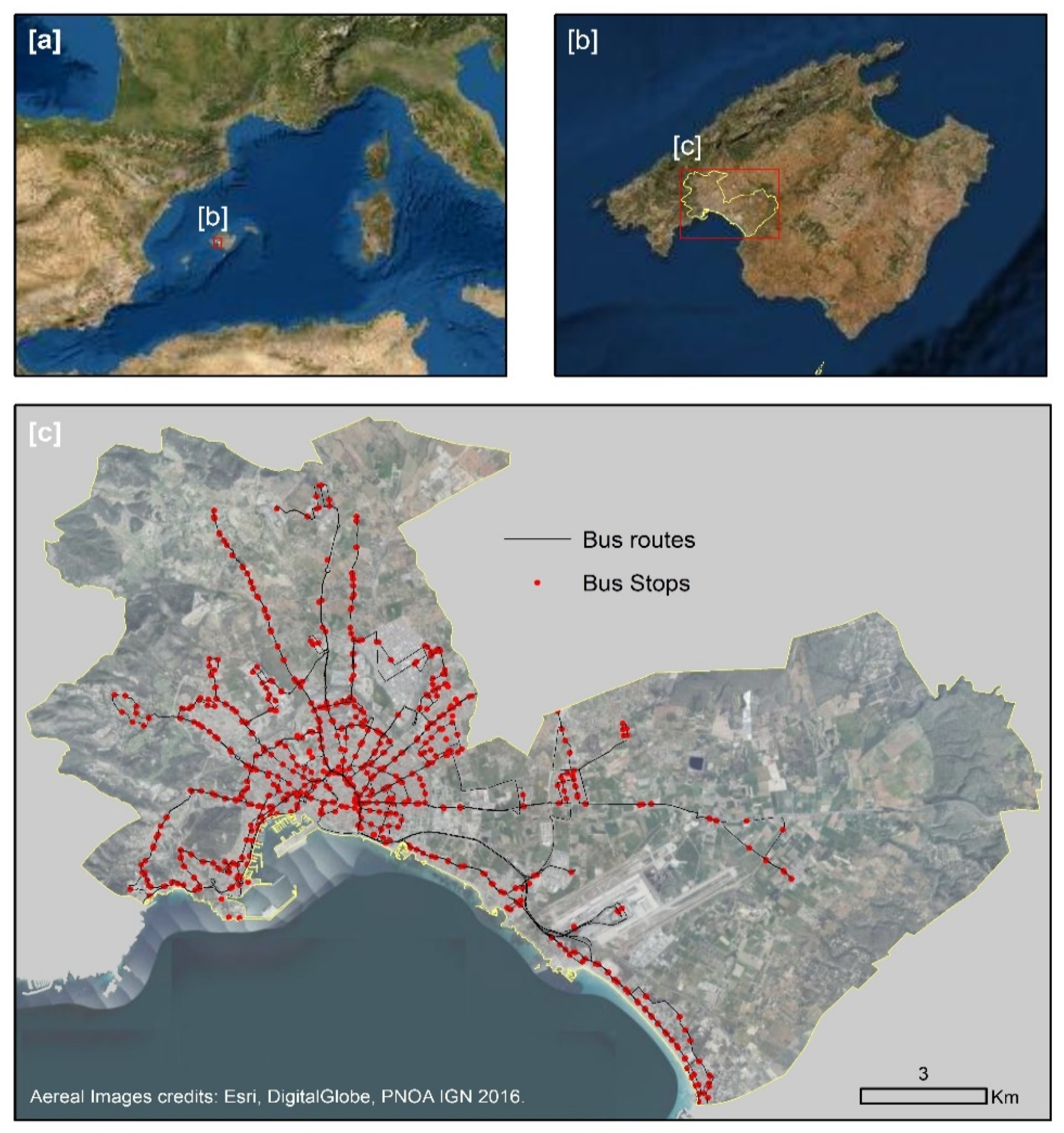
3.1. Case Study

The city of Palma is the capital of the Balearic Islands (Spain; see Figure 1a,b), with a total of 416,065 inhabitants [49] and a surface area of 208.63 m², which means a density of 1948.39 inhabitants/km². It is a highly populated city whose spatial distribution is not homogeneous (Figure 2).

The Empresa Municipal de Transports Urbans de Palma (EMT) [50] is the public company dependent on Palma Town Council, which is responsible for planning and managing urban bus transport. The EMT operates a total of 30 bus lines in Palma. The bus line distribution utilises a radial transport model, in which most routes converge at the Avenidas, a stretch of the road network that outlines the old city wall (Figure 1c).

In recent months, the EMT has launched new routes and new frequencies, which has given rise to intense social debate.

3.2. Data Sources

The following data sources were employed:

3.2.1. Geographic Zones and Population

Assessment of the influence of the MAUP on service and equity indicators was based on the consideration of four types of spatial units of reference: neighbourhoods, census sections, cadastral blocks, and a 400 × 400 m mesh (Figure 2). Their sources were as follows:

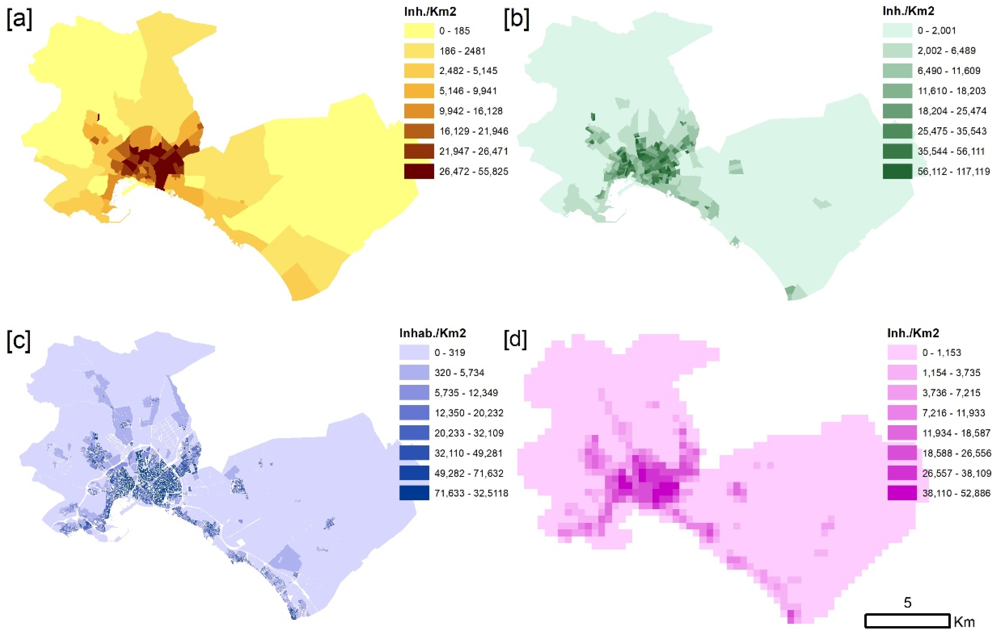
• Neighbourhoods—The division into neighbourhoods in Palma city was provided by the Population Service of Palma City Council. A total of 88 areas of heterogeneous dimensions were recorded.
• Census sections—The National Institute of Statistics is responsible for carrying out the population census in Spain, which it does every 10 years. A total of 245 census sections were recorded.
• Cadastral blocks—From Palma City Council, through its Department of Population. The municipality of Palma comprises a total of 3012 cadastral blocks.
• 400 × 400 m mesh—A mesh of homogeneous square polygonal units of dimensions 400 × 400 m was created. The municipality comprises a total of 1381 units. Its population was obtained from census sections.

Table 1. Description of the zones considered.

Indicators	Neighbourhoods	Census Sections	Cadastral Blocks	400 × 400 m Mesh
Nº Units	88	245	3012	1381
Minimum surface (HA)	4.35	1.53	0.01	16.00
Mean surface (HA)	222.08	79.66	6.10	16.00
Maximum surface (HA)	3771.88	3918.45	185.14	16.00
Standard deviation	509.92	318.40	55.53	0
Minimum population	0	0	0	0
Mean population	4786.29	1634.16	153.22	335.35
Maximum population	27,872	4430	2285	8461.72
Standard deviation population	4759.25	622.60	186.48	1050.72
Minimum population density	0	0	0	0
Mean population density (inhab/ha)	130.03	249.90	329.97	20.95
Maximum population density (inhab/ha)	558.24	1171.19	3251.17	528.85
Standard deviation Population density	118.78	241.64	391.26	65.67

includes descriptions of the different zoning metrics we have defined. It can be seen that there is significant variability in their characteristics. The geographical division into neighbourhoods is most commonly used at a social level by the Palma City Council to manage facilities and infrastructure. The census division is used to define electoral districts and has few connotations in the territorial planning of facilities. The division into cadastral blocks is used by the Town Hall’s Population Department, in order to manage the precise pattern of inhabitants and to provide support for social services. The 400 × 400 m mesh was chosen because it is common in transportation studies to use an area of influence of 400 m to calculate the bus service or accessibility to bus stops [26,51]. This type of zoning was also proposed to analyse the effects of orthogonal zoning.

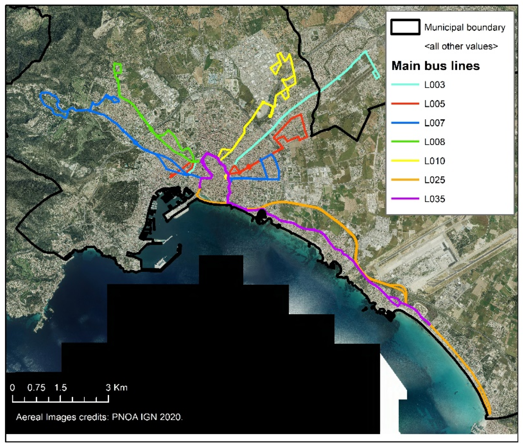
3.2.2. Bus Stops, Bus Lines, and Frequencies

The urban bus service network was provided by the Municipal Transport Company, through its Open Data portal. These data can be accessed in GTFS format (see Figure 1c). A total of 30 routes and 851 stops were considered. The average frequencies in a working day of the routes were obtained from the EMT website [50] (

Table 2. Bus lines and frequencies. Source: Empresa Municipal de Transports de Palma, 2020 [50].

Route	Frequency (min)	Route	Frequency (min)
L001	20	L019	30
L002	30	L020	20
L003	10	L023	30
L004	15	L024	22
L005	8	L025	20
L006	40	L027	15
L007	10	L028	30
L008	8	L029	20
L010	12	L031	20
L011	40	L033	20
L012	22	L035	10
L014	22	L039	20
L016	20	L046	20
L017/A1	20	L047	20
L018	60	A2	30

).

There is a high degree of overlapping between the routes, especially in the downtown area of Palma, which structurally conditions the level of service and accessibility of the city.

3.3. Methodology

The methodology proposed involves the integration of a Geographic Information System with a Simulation and Optimization Tool. For this purpose, the Arcmap v. 10.5 (©ESRI), Geoda 1.12 [52], and @Risk v. 6.0 (©Palisade) software were used. Products required to be included in the simulation and optimization system were generated through the GIS.

The methodological process developed is presented in Figure 3. Its objective is to analyse the effect of zoning on bus service level values and their equity in their distribution in the territory. For this purpose, a method for calculating BSL and equity is available, which was used for the four proposed zonings.

The tasks performed were as follows:

3.3.1. Calculation of the Bus Service Level and the Horizontal Equity Using the Current Bus Frequencies

To calculate the bus service level, the following tasks were carried out:

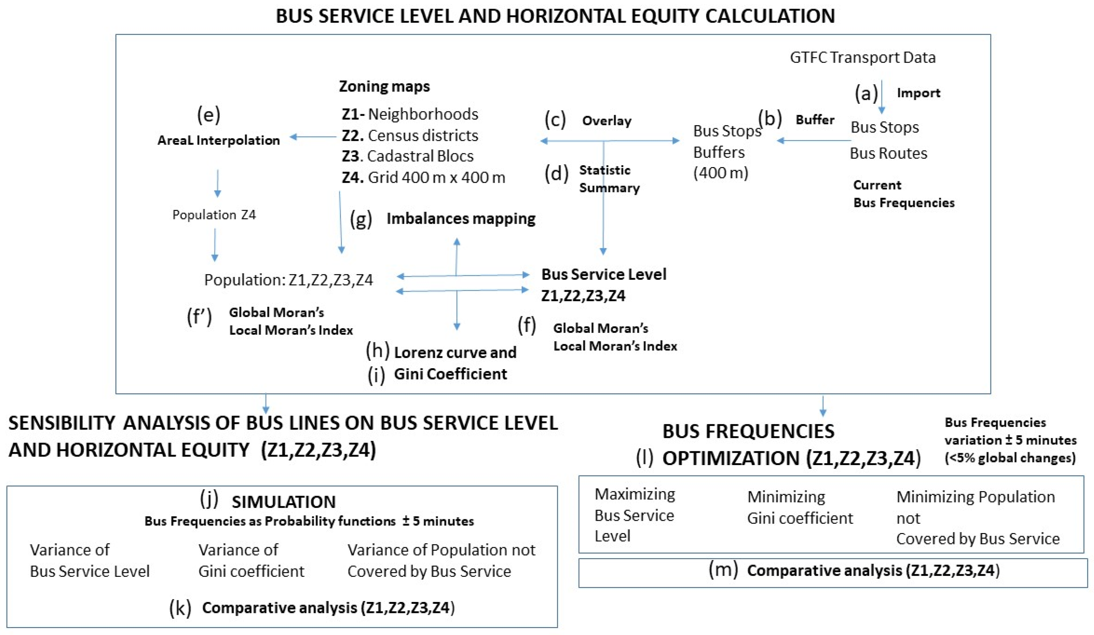
• GIS database creation—Importation of geographical transport files (GTFC), bus stops, and routes (Figure 3a).
• Calculation of the Bus Service Level by Bus Stop—The level of service provided by each bus stop was calculated based on the number of buses that pass through it over the course of 12 h, according to the following expression:

  $${Bus Service Level}_{ bs}={{\displaystyle \sum }}_{r=1}^s\frac{60}{{Freq}_r}12 \mathrm{h}.$$

  (1)

  bs = bus stop; r = bus route; s = total number of routes; Freq_r = Frequency of route r
• Calculation of the Bus Service Level (BSL) for each geographic unit—Using the DelBosc method [26], a buffer of 400 m was generated for each bus stop (Figure 3b) and the number of buses passing through this stop was counted. The buffer layer was then overlapped on each of the zonings carried out, obtaining a level of service for each geographical unit, according to the following expression (Figure 3c):

  $$Geographic Unit Service Level x={\displaystyle \sum }_{bs=1}^m\frac{{Area Buffer}_{ bs,x}}{{Area}_{ Geographic Unit x}}.$$

  (2)

  x = geographic unit; bs = bus stop; m = number of bus stops

This provided a service level value for each geographical unit, based on the number of buses passing through bus stops within 400 m. Therefore, an increase in the frequency of a line indicates a greater number of buses per bus stop, which serves to increase the service level of the geographical units within its area of influence.

A global bus service level indicator was then obtained, according to the following expression (Figure 3d):

$$Global Service Level= {\displaystyle \sum }_{g=1}^n{Geographic Unit Service Level}_g.$$

(3)

The horizontal equity analysis consisted of a comparative analysis of the resident population in each geographic unit, with respect to their level of bus service. Its calculation included the following tasks:

• Calculation of the population of the Grid 400 × 400 m mesh zoning—To calculate the mesh zoning population (Figure 3e), an aerial interpolation [53,54] was performed from the census districts zoning population map.
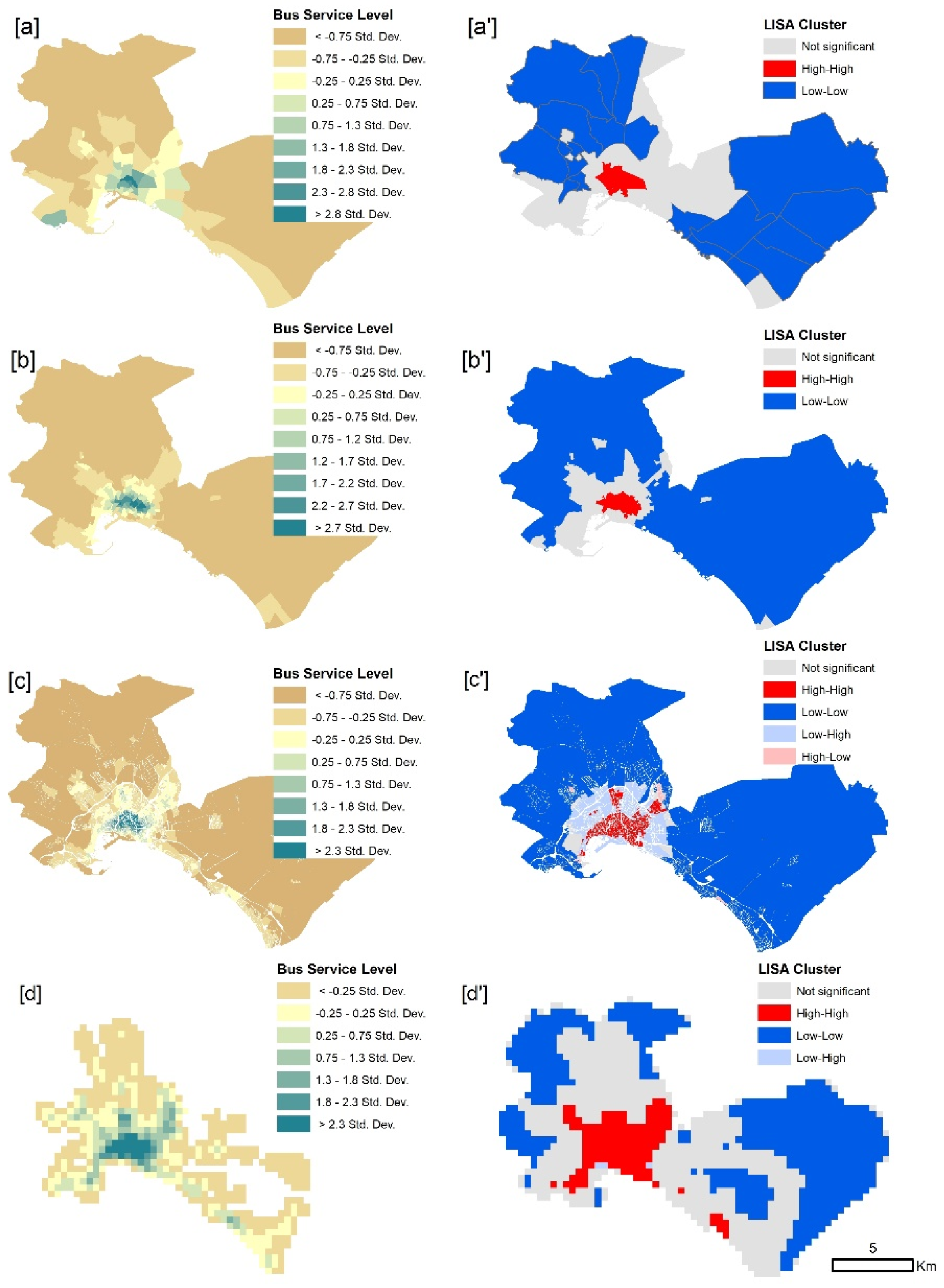
• Analysis of population concentration and bus service—An analysis of the spatial autocorrelation of the service level and population was carried out by calculating the Moran’s Global and Local indices [55,56,57]. The Moran’s Global index provides information on the spatial autocorrelation of the variable and its degree of concentration:

  $$I = \frac{N}{{{\displaystyle \sum }}_i{{\displaystyle \sum }}_j{w}_{ij}} \frac{{{\displaystyle \sum }}_i{{\displaystyle \sum }}_j{w}_{ij}\left(X_i- \overline{X}\right)\left(X_j- \overline{X}\right) }{{{\displaystyle \sum }}_i{\left(X_i- \overline{X} \right)}^2},$$

  (4)

  N = number of indexed spatial units by i, j; X = value of the variable; $\overline{X}$ = mean of X; W_ij = weighted matrix element, where a value of −1 indicates maximum dispersion, a value of 0 indicates a random distribution, while a value equal to 1 indicates a concentrated distribution. The Local Moran’s index is used to verify the concentration of the variable in space (Figure 3f,f′).

Spatial autocorrelation is subject to spatial heterogeneity, which recognizes a specific contribution of each point to the overall autocorrelation. The local autocorrelation was evaluated by local indicators of spatial association (LISA). The Local Moran’s I is a local spatial autocorrelation statistic that identifies local clusters or local outliers, in order to understand their contribution to the ‘global’ clustering statistic:

$$I_i= \left(\raisebox{1ex}{$z_i$}\!\left/ \!\raisebox{-1ex}{$m_2$}\right.\right) {\displaystyle \sum }_{j=1}^n{w}_{ij} z_j.$$

(5)

variance: $m_2$; z = mean deviation $\left(X_i-\overline{X}\right)\left(X_j- \overline{X}\right)$; W_ij = weighted matrix element.

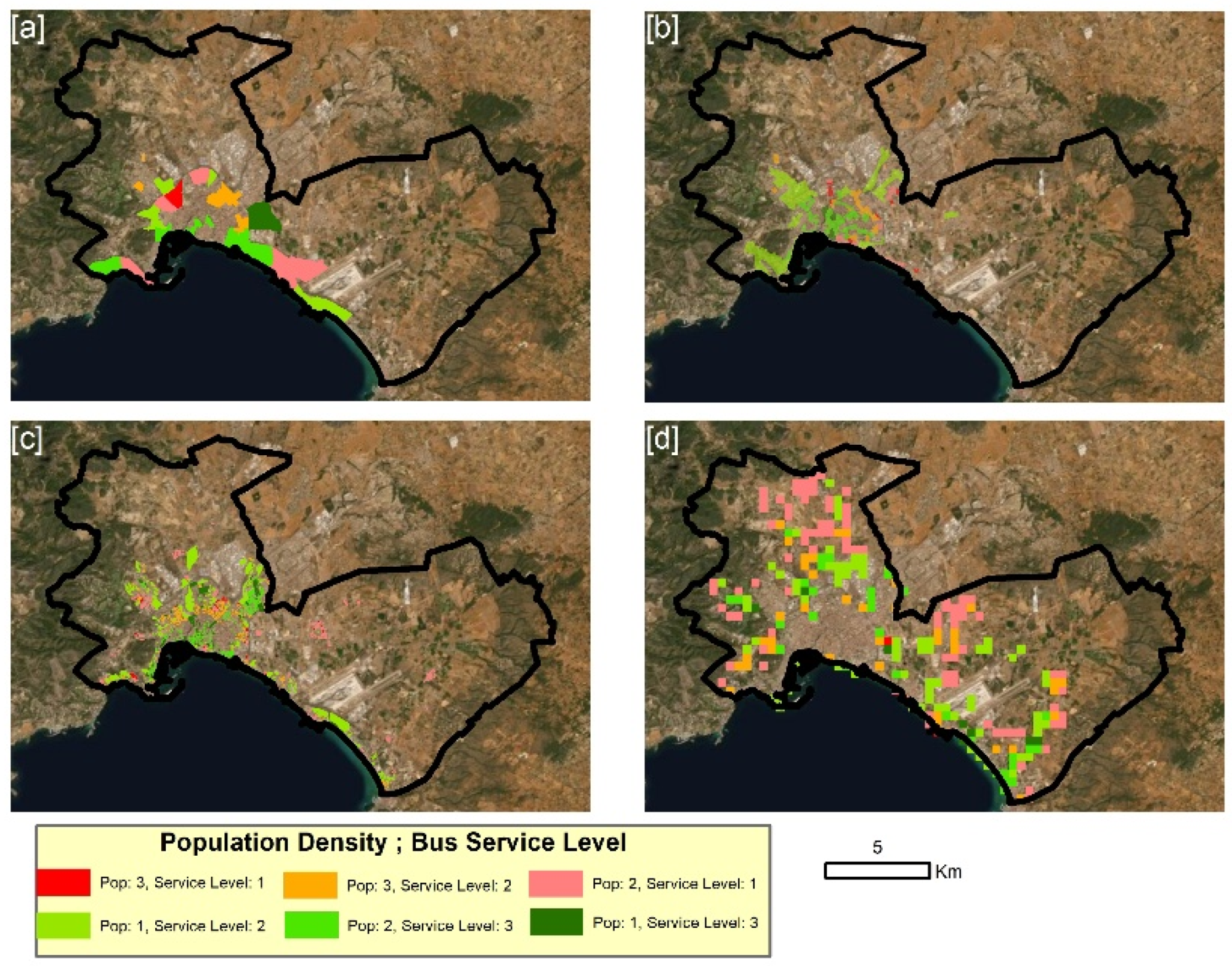
• Mapping of territorial imbalances (Figure 3g)—A cartographic analysis was performed for each type of zoning, in order to represent the relationship between the population and level of service. For this purpose, the mapping of the level of service normalized by resident population was presented and deficit zones were identified. The process is carried out by classifying the population and the level of service in three categories (33 and 66 percentile), and represented by a map showing all the categories.
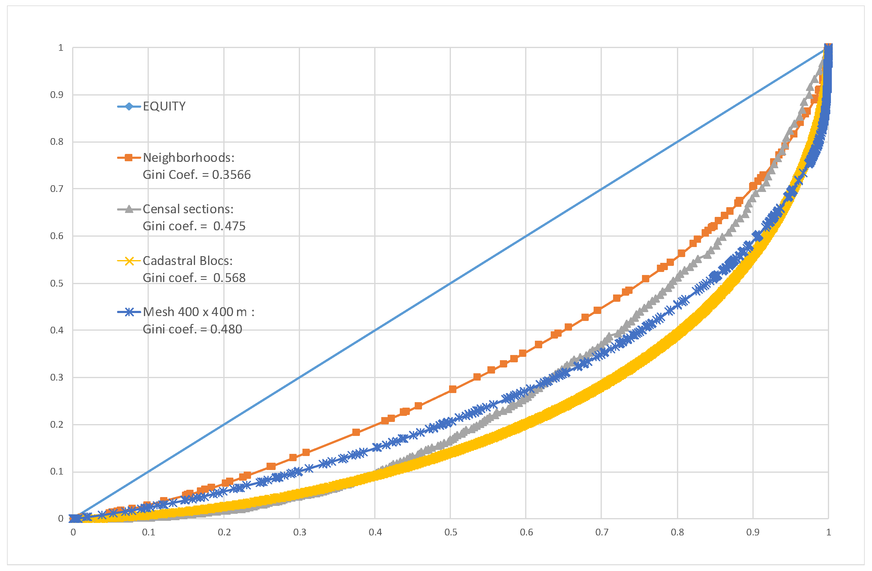
• Lorenz Curves generation (Figure 3h)—A Lorenz curve shows a cumulative distribution of the level of service and population for geographic units, as well as the straight line that would represent perfect equality in distribution [26,27]. A Lorenz curve was constructed for each of the zonings, based on the information corresponding to the population of each geographic unit and its level of service, in which the level of horizontal equity can be observed.
• Gini coefficient calculation—The Gini coefficient [26,58,59] was developed in the field of economics, in order to measure the degree of inequality of an economic variable (income) in relation to the population. The index is based on an analysis of the deviation from the Lorenz curve. The calculation of the Gini coefficient was carried out using accumulated population and service level data for each of the zonings used, according to the following expression (Figure 3i):

  $$Gini coefficient=1-{\displaystyle \sum }_{i=0}^n\left(\delta Y_{i-1}+\delta Y_i\right)\left(\delta X_{i-1}-\delta X_i\right).$$

  (6)

  i = row; n = number total of districts; Y = accumulated service level; X = accumulated population

The Gini coefficient ranges from 0, when there is no concentration of service (perfect equality), to 1, when there is an absolute concentration in one location (inequality).

The Gini indicator, therefore, makes it possible to relate the concentration of the bus service level to the geographical units considered. Thus, it is very sensitive to changes in bus frequencies, as changes in the service level of geographical units also alter their degree of concentration.

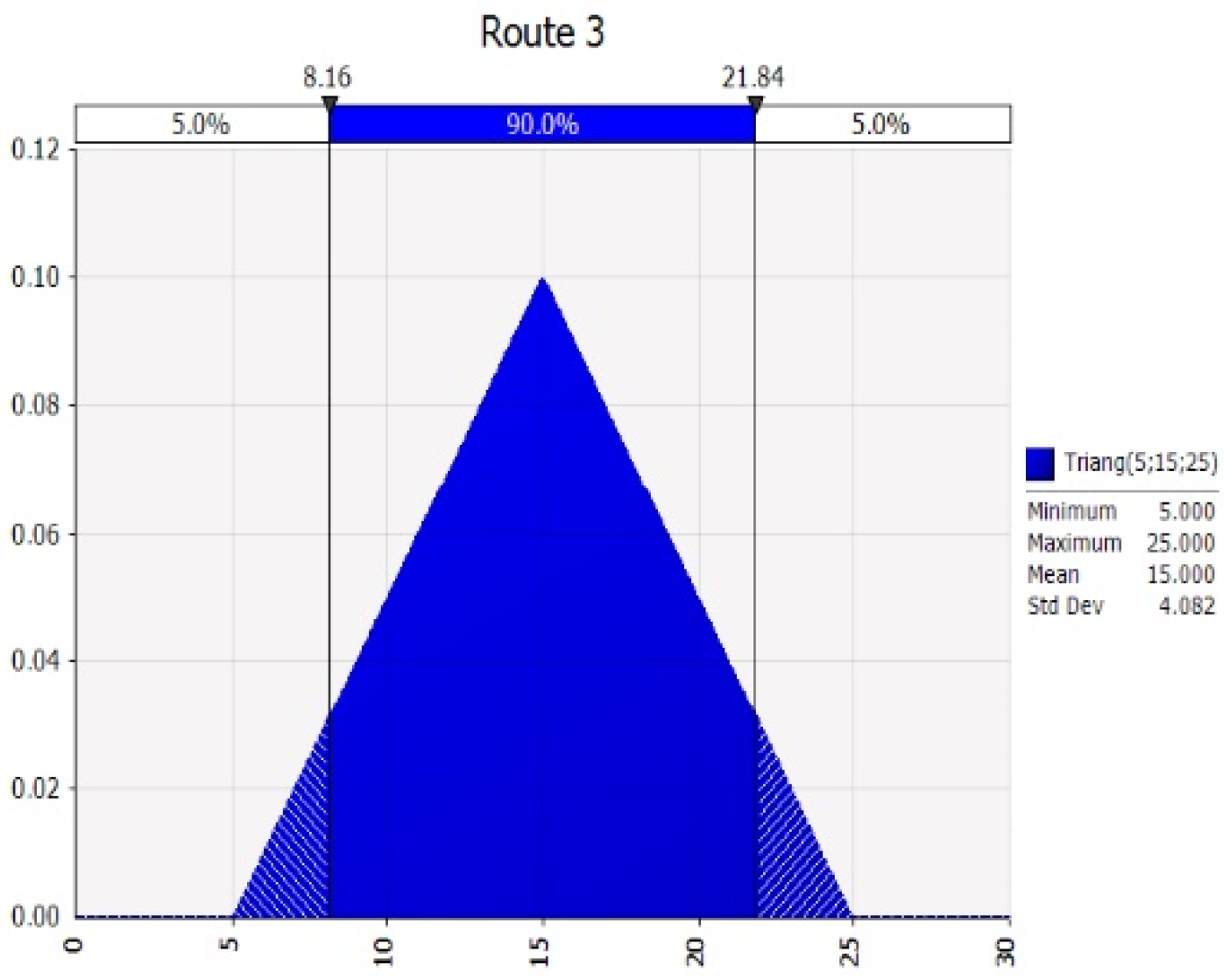
3.3.2. Sensibility Analysis of Bus Service Level and Horizontal Equity by Simulation of the Change of Bus Frequencies (±5 min)

A simulation process was carried out to evaluate the effect of changing the frequency of each bus line on the level of service and the level of horizontal equity (Figure 3j). The proposed sensitivity analysis was based on the modelling of bus line frequencies. In particular, we replaced the absolute value of their frequencies with a triangular-type probability statistical function that covers the possible range of frequency variability. Figure 4 shows a graph representing the function, assuming an average frequency of 15 min and a variability of 10.

By incorporating this statistical function into the calculation of the service level, the expression is as follows:

$$Bus Service Level bs= {{\displaystyle \sum }}_{r=1}^s\frac{60}{f{\left(Triang \left(a_{bs};c_{bs};b_{bs}\right) \right)}_r} 12 \mathrm{h}.$$

(7)

The simulation process was developed based on a Monte Carlo model that assigns random values to the frequencies of each bus line, assuming a maximum variability per line of ±5 min of the current frequency. The simulation process included a total of 10,000 interactions, allowing for a range of variability to be obtained for the service level values in each geographical unit, the overall bus service level, and the Gini coefficient.

In addition, a new variable “Population not covered by bus service” (PNC) was created from the combination of the bus service level and population values for each geographic unit. Specifically, bus service and population were classified into three categories (>=0 and <=33rd Percentile, >33rd Percentile and <66th Percentile, >66th Percentile) and the population of those geographical units whose population was at a percentile above the service level percentile was added (8).

Population = (1, 2, 3); Bus Service Level = (1, 2, 3)

$$\mathrm{PNC} = {{\displaystyle \sum }}_{i=1}^n{Population}_i \nabla {Population interval}_i>{BSL interval}_i$$

(8)

i = geographical unit; n = Number of geographical units

The combined results of the simulations performed for each zoning and each variable could be conveniently analysed through the construction of a table (see Figure 3k).

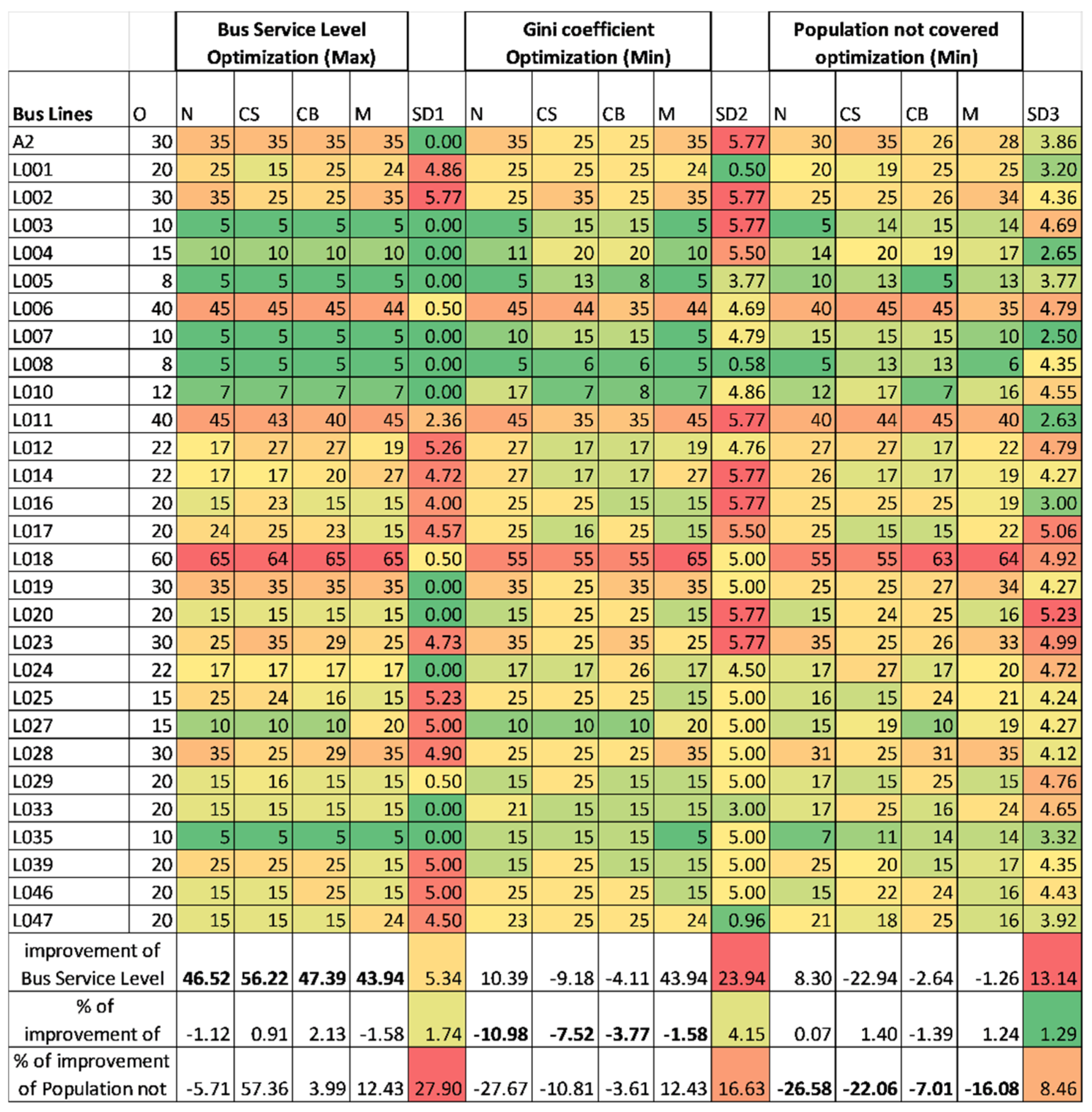
3.3.3. Optimization of Bus Fleet Frequencies

We used an optimization process to select the best combination of frequencies, in order to improve service and equity in each of the zonings. Our objective was to analyse the differences in the results and to test the influence of zoning on the results.

Three optimization processes were developed (Figure 3l):

• Maximising the Global Service Level;
• Minimisation of the Gini coefficient; and
• Minimisation of population not covered by the Bus Service.

At the level of model restrictions, it was considered appropriate not to allow a variability of more than ±5 min in the frequency of each line, taking into account that the total sum of frequencies would be around 5% of the current value. The minimum frequency of the lines was also limited to 5 min.

The combined results of the optimization performed for each zoning and each variable could be conveniently analysed through the construction of a table (see Figure 3m).

The modelling process was carried out using the @Risk v6.0 software and the Optimizer module (©Palisade) [60]. The optimization model incorporated a total of 10,000 iterations.

4. Results and Discussion

4.1. Service Level and Equity for Each Zoning with the Current Bus Frequencies

The bus service level estimated on the current frequencies for each type of zoning presented relatively homogeneous results. Figure 5a–d show the service level distribution for the four zonings considered. In all cases, the maximum values were concentrated in the central zone of the town centre. This area overlaps with the convergence zone of most of the city’s bus lines.

The overall Moran’s indices of the geographical distributions for the service level always obtained high values, which indicates a high level of geographical grouping (

Table 3. Global Moran’s Index; significance < 0.05.

	Neighbourhoods	Census Sections	Cadastral Blocks	400 × 400 m Mesh
Population	0.146	0.01	0	0.749
Density Population	0.471	0.328	0.239	0.749
Bus Service Level	0.669	0.820	0.829	0.809

). Such concentration was not as evident in the population’s distribution, as the values of the Moran’s index were significantly lower. However, the overall Moran’s values for the population density distribution did show concentrated patterns. This fact could be an essential clue to consider in bus demand analyses.

Zoning with smaller spatial units showed the detail of the variability of the service level distribution in different city areas. The loss of quality and refinement of information when scaling up was noticeable. An illustration of this is that the concentration of service in the southeast coastal area was only clearly identified within the cadastral and mesh block zonings (Figure 5c′,d′).

The Moran’s Local indexes represented in Figure 5a′–d′ show the service level concentration pattern. These maps represent the areas in which there is a significant positive autocorrelation between the geographical unit values and their environment (High–High) in red. The zoning shown in Figure 5 d′ (mesh) was the only one in which a concentration zone appears in the southeast of the municipality. This fact is not a trivial one; it reflects that orthogonal units allow spatial patterns to be identified with greater precision than smaller units, which are more adapted to urban morphology or demographic issues.

The horizontal Gini coefficient calculated for each zoning showed slightly differing results: neighbourhoods (0.3566), census sections (0.475), cadastral blocks (0.568), and mesh (0.48). Therefore, the different zonings showed significant differences in the comparative equity analysis. This was due to the different types of concentration of service level and population. Such variability is evidence of the modifiable spatial unit problem’s effect on the calculation of a transport service indicator.

Figure 6 shows the distribution of the Lorenz curves for the four zonings analysed. The graph represents the accumulated population (x-axis) and the accumulated bus service level (y-axis). Its observation allows us to identify more significant inequalities (distance from the diagonal line), when smaller units are used (Cadastral Blocks/Mesh). For zonings whose units were bigger (Neighbourhoods and cadastral blocks), better horizontal equity results were obtained. This fact is essential, as it would advise the planner to opt for the use of smaller geographical units, in order to assess the level of equity more accurately.

As the Gini coefficient is an overall indicator of equity, it is advisable to carry out a more detailed geographical analysis of the relationships between service level and population.

Figure 7 shows the imbalances between the level of service and the population for the different zonings. We can observe that, as the size of the geographical unit is reduced, the areas that present more deficiencies or excesses in the bus level of service concerning their population can be identified more precisely. We also note that the cadastral block zoning showed a great deal of detail, in terms of deficit and excess transport service with respect to the resident population. The mesh zoning (Figure 7d) has great potential to detect territorial imbalances in a global way throughout the municipal territory. Its level is not detailed; however, it does indicate areas where the service should be enhanced in various zones that did not appear in the other zonings. It is important to note that the results obtained were different for each type of zoning.

4.2. The Role of Bus Lines in Service Level and Horizontal Equity

The simulation process allowed us to analyse each bus line’s role, concerning the level of BSL and horizontal equity. Figure 8 shows the variance values of the BSL, the Gini coefficient, and the PNC derived from the frequency variations of each bus line under all of the zonings. The sign of the values represents the effect that varying bus line frequencies will have on the BSL, Gini coefficient, and PNC; a negative sign indicates that an increase in the frequency of the line (i.e., more significant number of buses per hour) will result in a decrease in the BSL, a decrease in the Gini coefficient (more significant equity), and a lower PNC. A positive sign implies that an increase in line frequency will result in higher BSL, an increase in the Gini coefficient (inequality), and an increase in PNC. The absolute value indicates the degree of variance explained in the variables (i.e., BSL, Gini coefficient, and PNC) by a variation in the frequency of each line. The values of the BSL were always positive; therefore, whenever there is an increase in the frequency of any line, the result will be positive on the BSL. For the Gini coefficient, however, positive and negative values were observed. This indicates that an increase in frequency on certain lines may positively or negatively affect the Gini coefficient; in other words, increasing frequencies on certain lines can cause imbalances. This is as increases in the BSL in areas with low demand can cause inequality. The same situation occurred with respect to the PNC values.

The table also shows several columns, including the standard deviation (SD) of the variance explained by each bus line for each variable (BSL, Gini coefficient, and PNC) and zoning. High deviation values show changes in the roles of these lines for each of the zonings analysed.

When zoning by neighbourhoods, the level of service depended primarily on lines 7 (39.85%), 35 (13.03%), 5 (8.93 %), and 3 (7.13%) which concentrated most of the variance. When zoning by census tracts, the priority lines were 7 (35.86%), 5 (22.94%), 3 (15.97%), and 8 (11.38%). The top priority lines that explained the greatest variance when zoning by Cadastral Blocks were 7 (40.22%), 5 (14.61%), 35 (12.82%), and 3 (10.07%). For the 400 × 400 mesh zoning, the main lines were 7 (38.28%), 35 (14.14%), 5 (9.56%), and 8 (8.58%). The standard deviation of the explained variance for each line in each zoning indicates that lines 5 (6.47), 35 (6.36), 8 (4.81), and 3 (4.17) were those that showed the highest values. The rest of the lines obtained similar values.

In the case of the Gini coefficient, greater variability was observed both in the signs and the magnitudes of the variances. When zoning by neighbourhoods, the lines that obtained greater significance were 5 (−44.05%) and 8 (−10.39), whose increase in frequency implied a reduction in the Gini coefficient (thus leading to more equity); while lines 35 (14.18%) and 10 (3.94%) went in the opposite direction (i.e., an increase in frequency would result in less equity). When zoning by census tracts, the lines that improved equity were 10 (−28.14%) and 8 (−26.48%), while those that decreased it were 5 (19.29%) and 4 (8.79%). When zoning by Cadastral Blocks, the balancing lines were 8 (−5.82%) and 39 (−5.23%), while the unbalancing ones were 35 (38.90%), 7 (10.69%), and 4 (10.35%). Under the 400 × 400 m mesh division, the decrease of the Gini coefficient came from lines 5 (−32%) and 8 (−11.91%), while its increase came from 35 (18.39%) and 25 (5.97). The standard variation, in this case, was maximum for lines 5 (29.5), 35 (15.15), and 10 (14.48), and maintained significant variabilities for the rest of the lines.

The role of the lines in the percentage of uncovered population by bus service also showed significant variability. When zoning by neighbourhoods, the lines that reduced the population not covered were 3 (−24.52%) and 5 (−12.07), while those that increased it slightly were 12 (2.28%) and 35 (2.21%). When zoning by census tracts, no line was clearly identified that could improve service coverage; however, the increase in frequency of lines 7 (39.61%), 5 (24.37%), and 3 (14.02%) worsened it. When zoning by Cadastral Blocks, lines 12 (−2.71%) and 24 (−2.36%) reduced the imbalances, while lines 35 (23.40%) and 3 (13.35%) increased them. Under the zoning of the 400 × 400 m mesh, increases in lines 35 (−10.95%) and 7 (−7.06%) decreased the amount of population with imbalances, while lines 10 (8.24%) and 27 (2.96%) increased it. The standard deviation showed large variability for lines 7 (20.69), 3 (−18.02), 5 (15.4), and 35 (14.31).

The results show that the choice of zoning has significant consequences on identifying priority lines for the improvement of the level of service and equity. Therefore, frequency planning in bus fleet management should be based on an exhaustive knowledge of the effect caused by the variation of each line at various scales of analysis. Increasing frequencies on a line always result in improved service levels; however, it can also result in imbalances, which must be known. As we saw in the previous section, zonings with smaller units are more accurate and sensitive to detecting frequency modification effects; however, when we analysed the effects of frequency variation in detail, we obtained different results, which did not justify the advantages of one or the other zoning.

The results show that Palma city’s bus service depends fundamentally on a reduced set of lines. These are very long lines, which include many stops, deployed throughout the city in a radial route (Figure 9). Therefore, this is a very unbundled transport model that is very vulnerable to imbalances caused by inadequate frequency management. In these cases, it may be advisable to disaggregate the routes into shorter independent itineraries, which allow for both radial and transversal access throughout the city.

4.3. Bus Frequencies Optimization to Improve Service Level and Horizontal Equity

The optimization of bus line frequencies to maximize the level of service and horizontal equity showed slightly different results, depending on the type of zoning used. The optimization assumed frequency oscillations of ±5 min per bus line, as long as the total variation of the original frequency did not exceed 5%.

Figure 10 shows the main results of the optimization process. The values show the frequency (in minutes) proposed for each line, in order to optimize the BSL, Gini coefficient, and the PNC under the different zonings (N, CS, CB, and M). The last three rows summarise the optimization results as a percentage.

It can be seen that the optimization of the bus service level provided improvement values between 43% and 56%, depending on the type of zoning used (with a standard deviation of 5.34 min). In this case, significant variability of the frequencies assigned to lines 2, 12, 25, 46, 39, and 27 was observed for each type of zoning, although lines 3, 4, 5, 7, 8, 19, and 35 maintained constant low frequencies.

The optimization of horizontal equity through the minimization of the Gini coefficient did not lead to improvements of lesser magnitude than for service level. The improvement values obtained for each type of zoning ranged from −10.98% (at the neighbourhood level) to −1.58% (at the 400 × 400 m mesh level). These values were significantly lower than for BSL. This implies that the service model is somewhat limited, in terms of improvement, by the current distribution of its lines in general; that is, it is inelastic and cannot easily be improved. In this case, the standard deviation of most lines was significant. This implies that the optimization results were very different for each type of zoning.

The unmet demand reduction optimization results showed the possibility of improvements, ranging from 7% (CB) to 26% (N). Furthermore, the variability of line frequencies was very varied for each of the zonings used.

The results demonstrate the significant variability of optimization results, depending on the type of zoning used and the optimized variable (i.e., NS, Gini coefficient, PNC). In general, Neighbourhood zoning tended to magnify the effects of optimization (46% NS, −10.98 Gini, −26.58 PNC). The rest of the zonings provided very different results. The mesh zoning provided smaller improvement values for NS and Gini, thus smoothing the improvements. Therefore, it was not possible to identify the best type of zoning, based on these results.

5. Conclusions

The problem of the modifiable spatial unit must be adequately considered in the process of transport and mobility planning. The type of zoning used determines the values of Bus Service Levels and equity indicators. This can lead to the detection of erroneous territorial imbalances, which may result in unjustified investments.

From the case study of the city of Palma, the following conclusions were drawn:

• Small unit zoning is much more accurate for service-level analysis. Small units are also more sensitive to detecting imbalances between bus service supply and resident population levels.
• The range of variability of global indicators of concentration (Moran’s Global) did not undergo very significant changes, concerning the use of various zonings; in other words, service level concentrations were detected in all cases. However, the identification of the high bus service level areas (Moran’s Local) was more precise when using small unit zoning. The use of large units can hide significant areas of concentration.
• Orthogonal zoning (mesh) proved to be particularly sensitive for concentration detection, regardless of unit size. It has a tendency to soften the values of BSL improvement and equity, compared to the other zonings. At the same time, it provides a broader view of the municipality.
• The horizontal equity analysis showed that the Gini coefficient increases as the size of the geographical units decreases. This implies that the smaller the geographical unit used, the greater the sensitivity in detecting imbalances. In other words, many imbalances could go undetected if large geographical units are used.
• The sensitivity analysis of bus service level and equity derived from the variation of route frequencies showed the strong dependence of service level on a series of long-distance routes that radially cross the city. This bus transportation system demonstrates rigidity.
• There were significant variations in the roles of bus lines, depending on the type of zoning used. In general, there was a coincidence in the zoning systems, in terms of identifying the lines that improve the level of service. However, there were significant divergences for the maintenance of equity; these issues are unclear.
• In optimizing the level of service and horizontal equity by changing the frequencies of bus lines, it became clear that fundamental changes must be made to the city’s key lines. The variations to the original service level values are significant and can lead to improvements in many areas.

It is convenient to focus the analysis of transport from a scalar perspective at a global level, considering different zonings to extract results jointly. The use of a particular zoning can obscure the processes of service concentration and imbalances, which must be identified. The planner must be very careful with the value obtained from the used indicators. These indicators cannot, in any case, be generalized for the geographical area analysed, and are closely related to the zoning used.

Bus transport systems in a city can be very dependent on some key lines. By using simulation techniques, it is possible to detect these lines and model them properly, in order to improve the service level.

The transport system’s intrinsic configuration limits the possibilities of optimization by modifying the frequencies of its lines. The margin for improvement is relatively small using this technique. It can provide advantages, however, as it does not require any further investment in infrastructure.

The modifiable spatial unity problem must necessarily be considered in the planning of public bus transport. A multiscale geographical vision is required to obtain a rigorous global diagnosis of service and equity level. The indicators obtained must be sufficiently validated by geographical analysis, in order to properly be used as decision tools at various scales.

The combined use of Geographic Information Systems and simulation and optimization tools is a fundamental tool for the transport planner. In this sense, it is desirable that GIS software packages soon incorporate simulation tools in this area.

References

1. Levine, C. The concept of vulnerability in disaster research. J. Trauma. Stress 2004, 17, 395–402. [Google Scholar] [CrossRef]
2. Fotheringham, A.S.; Wong, D.W.S. The modifiable areal unit problem in multivariate statistical analysis. Environ. Plan. A 1991, 23, 1025–1044. [Google Scholar] [CrossRef]
3. Openshaw, S. Ecological fallacies and the analysis of areal census data (UK, Italy). Environ. Plan. A 1984, 16, 17–31. [Google Scholar] [CrossRef] [PubMed] [Green Version]
4. Pereira, R.H.M.; Banister, D.; Schwanen, T.; Wessel, N. Distributional effects of transport policies on inequalities in access to opportunities in Rio de Janeiro. J. Transp. Land Use 2019, 12, 741–764. [Google Scholar] [CrossRef] [Green Version]
5. Mitra, R.; Buliung, R.N. Built environment correlates of active school transportation: Neighborhood and the modifiable areal unit problem. J. Transp. Geogr. 2012, 20, 51–61. [Google Scholar] [CrossRef]
6. Röthlisberger, V.; Zischg, A.P.; Keiler, M. Identifying spatial clusters of flood exposure to support decision making in risk management. Sci. Total Environ. 2017, 598, 593–603. [Google Scholar] [CrossRef] [Green Version]
7. Wang, C.; Quddus, M.A.; Ryley, T.; Enoch, M.; Davison, L. Spatial models in transport: A review and assessment of methodological issues. In Proceedings of the 91st Annual Meeting of the Transportation Research Board, Washington, DC, USA, 22–26 January 2012; Volume 750. [Google Scholar] [CrossRef]
8. Biehl, A.; Ermagun, A.; Stathopoulos, A. Community mobility MAUP-ing: A socio-spatial investigation of bikeshare demand in Chicago. J. Transp. Geogr. 2018, 66, 80–90. [Google Scholar] [CrossRef]
9. Viegas, J.M.; Martínez, L.M.; Silva, E.A. Effects of the modifiable areal unit problem on the delineation of traffic analysis zones. Environ. Plan. B Plan. Des. 2009, 36, 625–643. [Google Scholar] [CrossRef] [Green Version]
10. Litman, T. Evaluating Transport Equity. World Transp. Policy Pract. 2002, 8, 50–65. [Google Scholar]
11. Ruiz, M.; Segui-Pons, J.M.; Mateu-LLadó, J. Improving Bus Service Levels and social equity through bus frequency modelling. J. Transp. Geogr. 2017, 58, 220–233. [Google Scholar] [CrossRef]
12. Eisenberg-Guyot, J.; Moudon, A.V.; Hurvitz, P.M.; Mooney, S.J.; Whitlock, K.B.; Saelens, B.E. Beyond the bus stop: Where transit users walk. J. Transp. Heal. 2019, 14, 100604. [Google Scholar] [CrossRef] [PubMed]
13. Corazza, M.V.; Favaretto, N. A methodology to evaluate accessibility to bus stops as a contribution to improve sustainability in urban mobility. Sustainability 2019, 11, 803. [Google Scholar] [CrossRef] [Green Version]
14. Laasasenaho, K.; Lensu, A.; Lauhanen, R.; Rintala, J. GIS-data related route optimization, hierarchical clustering, location optimization, and kernel density methods are useful for promoting distributed bioenergy plant planning in rural areas. Sustain. Energy Technol. Assess. 2019, 32, 47–57. [Google Scholar] [CrossRef]
15. Kallel, A.; Serbaji, M.M.; Zairi, M. Using GIS-Based Tools for the Optimization of Solid Waste Collection and Transport: Case Study of Sfax City, Tunisia. J. Eng. 2016. [Google Scholar] [CrossRef] [Green Version]
16. Krichen, S.; Faiz, S.; Tlili, T.; Tej, K. Tabu-based GIS for solving the vehicle routing problem. Expert Syst. Appl. 2014, 41, 6483–6493. [Google Scholar] [CrossRef]
17. Kucuksari, S.; Khaleghi, M.A.; Hamidi, M.; Zhang, Y.; Szidarovszky, F.; Bayraksan, G.; Son, J.Y. An Integrated GIS, optimization and simulation framework for optimal PV size and location in campus area environments. Appl. Energy 2014, 113, 1601–1613. [Google Scholar] [CrossRef]
18. Li, X.; Chen, Y.; Liu, X.; Li, D.; He, J. Concepts, methodologies, and tools of an integrated geographical simulation and optimization system. Int. J. Geogr. Inf. Sci. 2011, 25, 633–655. [Google Scholar] [CrossRef] [Green Version]
19. Santé-Riveira, I.; Crecente-Maseda, R.; Miranda-Barrós, D. GIS-based planning support system for rural land-use allocation. Comput. Electron. Agric. 2008, 63, 257–273. [Google Scholar] [CrossRef]
20. Hadas, Y. Assessing public transport systems connectivity based on Google Transit data. J. Transp. Geogr. 2013, 33, 105–116. [Google Scholar] [CrossRef]
21. Porter, J.D.; Kim, D.S.; Ghanbartehrani, S. Proof of Concept: GTFS Data as a Basis for Optimization of Oregon’s Regional and Statewide Transit Networks; No. FHWA-OR-RD-14-12; Oregon Department of Transportation Research Section: Salem, OR, USA, 2014.
22. Sun, F.; Samal, C.; White, J.; Dubey, A. Unsupervised Mechanisms for Optimizing On-Time Performance of Fixed Schedule Transit Vehicles. In Proceedings of the 2017 IEEE International Conference on Smart Computing (SMARTCOMP), Hong Kong, China, 29–31 May 2017. [Google Scholar] [CrossRef]
23. Owens, S. From ‘predict and provide’ to ‘predict and prevent’? Pricing and planning in transport policy. Transp. Policy 1995, 2, 43–49. [Google Scholar] [CrossRef]
24. Lucas, K. Transport and social exclusion: Where are we now? Transp. Policy 2012, 20, 105–113. [Google Scholar] [CrossRef]
25. Boisjoly, A.; El-Geneidy, G. Public transport equity outcomes through the lens of urban form. In Urban Form and Accessibility; Elsevier: Amsterdam, The Netherlands, 2021; pp. 223–241. [Google Scholar]
26. Delbosc, A.; Currie, G. Using Lorenz curves to assess public transport equity. J. Transp. Geogr. 2011, 19, 1252–1259. [Google Scholar] [CrossRef]
27. Delbosc, A.; Currie, G. The spatial context of transport disadvantage, social exclusion and well-being. J. Transp. Geogr. 2011, 19, 1130–1137. [Google Scholar] [CrossRef]
28. Ferguson, E.M.; Duthie, J.; Unnikrishnan, A.; Waller, S.T. Incorporating equity into the transit frequency-setting problem. Transp. Res. Part A Policy Pract. 2012, 46, 190–199. [Google Scholar] [CrossRef]
29. Pereira, R.H.M.; Schwanen, T.; Banister, D. Distributive justice and equity in transportation. Transp. Rev. 2017, 37, 170–191. [Google Scholar] [CrossRef]
30. Lucas, K.; van Wee, B.; Maat, K. A method to evaluate equitable accessibility: Combining ethical theories and accessibility-based approaches. Transportation 2016, 43, 473–490. [Google Scholar] [CrossRef] [Green Version]
31. El-Geneidy, A.; Levinson, D.; Diab, E.; Boisjoly, G.; Verbich, D.; Loong, C. The cost of equity: Assessing transit accessibility and social disparity using total travel cost. Transp. Res. Part A Policy Pract. 2016, 91, 302–316. [Google Scholar] [CrossRef] [Green Version]
32. Liu, C.; Duan, D. Spatial inequality of bus transit dependence on urban streets and its relationships with socioeconomic intensities: A tale of two megacities in China. J. Transp. Geogr. 2020, 86, 102768. [Google Scholar] [CrossRef]
33. Aman, J.J.C.; Smith-Colin, J. Transit Deserts: Equity analysis of public transit accessibility. J. Transp. Geogr. 2020, 89, 102869. [Google Scholar] [CrossRef]
34. Mendiola, L.; González, P.; Cebollada, À. The relationship between urban development and the environmental impact mobility: A local case study. Land Use Policy 2015, 43, 119–128. [Google Scholar] [CrossRef]
35. Barboza, M.H.C.; Carneiro, M.S.; Falavigna, C.; Orrico, R. Balancing time: Using a new accessibility measure in Rio de Janeiro. J. Transp. Geogr. 2021, 90, 02924. [Google Scholar] [CrossRef]
36. Guo, Y.; Chen, Z.; Stuart, A.; Li, X.; Zhang, Y. A systematic overview of transportation equity in terms of accessibility, traffic emissions, and safety outcomes: From conventional to emerging technologies. Transp. Res. Interdiscip. Perspect. 2020, 4, 100091. [Google Scholar] [CrossRef]
37. Mooney, J.S.; Hosford, K.; Howe, B.; Yan, A.; Winters, M.; Bassok, A.; Hirsch, A.J. Freedom from the station: Spatial equity in access to dockless bike share. J. Transp. Geogr. 2019, 74, 91–96. [Google Scholar] [CrossRef] [PubMed]
38. Braun, L.M.; Rodriguez, D.A.; Gordon-Larsen, P. Social (in)equity in access to cycling infrastructure: Cross-sectional associations between bike lanes and area-level sociodemographic characteristics in 22 large U.S. cities. J. Transp. Geogr. 2019, 80, 102544. [Google Scholar] [CrossRef]
39. Sharma, I.; Mishra, S.; Golias, M.M.; Welch, T.F.; Cherry, C.R. Equity of transit connectivity in Tennessee cities. J. Transp. Geogr. 2020, 86, 102750. [Google Scholar] [CrossRef]
40. Manrique, J.; Cordera, R.; Moreno, E.G.; Oreña, B.A. Equity analysis in access to Public Transport through a Land Use Transport Interaction Model. Application to Bucaramanga Metropolitan Area-Colombia. Res. Transp. Bus. Manag. 2020, 100561. [Google Scholar] [CrossRef]
41. Romero, N.; Nozick, L.K.; Xu, N. Hazmat facility location and routing analysis with explicit consideration of equity using the Gini coefficient. Transp. Res. Part E Logist. Transp. Rev. 2016, 89, 165–181. [Google Scholar] [CrossRef]
42. Park, C.; Chang, J.S. Spatial equity of excess commuting by transit in Seoul. Transp. Plan. Technol. 2020, 43, 101–112. [Google Scholar] [CrossRef]
43. Banister, D. The sustainable mobility paradigm. Transp. Policy 2008, 15, 73–80. [Google Scholar] [CrossRef]
44. Horner, M.W.; Murray, A.T. Excess commuting and the modifiable areal unit problem. Urban Stud. 2002, 39, 131–139. [Google Scholar] [CrossRef]
45. Kwan, M.P.; Weber, J. Scale and accessibility: Implications for the analysis of land use-travel interaction. Appl. Geogr. 2008, 28, 110–123. [Google Scholar] [CrossRef]
46. Xu, P.; Huang, H.; Dong, N.; Abdel-Aty, M. Sensitivity analysis in the context of regional safety modeling: Identifying and assessing the modifiable areal unit problem. Accid. Anal. Prev. 2014, 70, 110–120. [Google Scholar] [CrossRef] [PubMed]
47. Pani, A.; Sahu, P.K.; Chandra, A.; Sarkar, A.K. Assessing the extent of modifiable areal unit problem in modelling freight (trip) generation: Relationship between zone design and model estimation results. J. Transp. Geogr. 2019, 80, 102524. [Google Scholar] [CrossRef]
48. Neutens, T. Accessibility, equity and health care: Review and research directions for transport geographers. J. Transp. Geogr. 2015, 43, 14–27. [Google Scholar] [CrossRef]
49. Instituto Nacional de Estadística (INE). Available online: https://www.ine.es/ (accessed on 15 December 2020).
50. Empresa Municipal de Transports Urbans de Palma. Available online: http://www.emtpalma.cat/en/home/ (accessed on 15 December 2020).
51. El-Geneidy, A.; Grimsrud, M.; Wasfi, R.; Tétreault, P.; Surprenant-Legault, J. New evidence on walking distances to transit stops: Identifying redundancies and gaps using variable service areas. Transportation 2014, 41, 193–210. [Google Scholar] [CrossRef]
52. Anselin, L. An Introduction to Spatial Autocorrelation Analysis with GeoDa. GeoDa Documentation. 2002. Available online: http://www.csiss.org/clearinghouse/GeoDa/ (accessed on 1 December 2020).
53. Goodchild, F.M.; Anselin, L.; Deichmann, U. A framework for the areal interpolation of socioeconomic data. Environ. Plan. A 1993, 25, 383–397. [Google Scholar] [CrossRef]
54. Hawley, K.; Moellering, H. A comparative analysis of areal interpolation methods. Cartogr. Geogr. Inf. Sci. 2005, 32, 411–423. [Google Scholar] [CrossRef]
55. Talen, E.; Anselin, L. Assessing spatial equity: An evaluation of measures of accessibility to public playgrounds. Environ. Plan. A 1998, 30, 595–613. [Google Scholar] [CrossRef] [Green Version]
56. Anselin, L. Exploring Spatial Data with GeoDA: A Work Book; Center for Spatially Integrated Social Science, University of Illinois: Chicago, IL, USA, 2005. [Google Scholar]
57. Rey, S.J.; Anselin, L. PySAL: A Python library of spatial analytical methods. In Handbook of Applied Spatial Analysis; Springer: Berlin/Heidelberg, Germany, 2010; pp. 175–193. [Google Scholar]
58. Ricciardi, A.M.; Xia, J.C.; Currie, G. Exploring public transport equity between separate disadvantaged cohorts: A case study in Perth, Australia. J. Transp. Geogr. 2015, 43, 111–122. [Google Scholar] [CrossRef]
59. Sitthiyot, T.; Holasut, K. A simple method for measuring inequality. Palgrave Commun. 2020, 6, 1–9. [Google Scholar] [CrossRef]
60. Palisade Corporation. @Risk: Risk Analysis Software Using Monte Carlo Simulation; Palisade Corporation: Ithaca, NY, USA, 2012. [Google Scholar]
Figure 1. (a) Location of Palma municipality in the Mediterranean basin; (b) Location of Palma municipality on Mallorca island; and (c) Bus stops and bus lines of the public network [50].
Ijgi 10 00111 g001
Figure 2. Population density of the municipality of Palma: (a) Neighbourhoods; (b) Census sections; (c) Cadastral blocks; and (d) 400 × 400 m mesh.
Ijgi 10 00111 g002
Figure 3. Methodological process.
Ijgi 10 00111 g003
Figure 4. Triangular probability distribution of the frequency of route 3 (a = 5 min; b = 15 min; c = 25 min).
Ijgi 10 00111 g004
Figure 5. Bus service level and Local Moran’s distribution (significance < 0.05): (a,a′) Neighbourhoods; (b,b′) Census sections; (c,c′) Cadastral blocks; and (d,d′) 400 × 400 m mesh.
Ijgi 10 00111 g005
Figure 6. Lorenz curve of the distribution of the bus service level and Gini coefficients.
Ijgi 10 00111 g006
Figure 7. Imbalances between service level and population: (a) Neighbourhoods; (b) Census sections; (c) Cadastral blocks; and (d) 400 × 400 m mesh.
Ijgi 10 00111 g007
Figure 8. Explained percentage of variance on Bus Service Level, Gini coefficient, and Uncovered Population, derived from bus frequencies variation. [N] Neighbourhoods; [CS] Census sections; [CB] Cadastral blocks; [M] 400 × 400 m mesh. [SD1], [SD2], and [SD3] Standard Deviation of the variance for each line for BSL, Gini coef., and PNC, respectively. Bus line A2 was not included, due to its low significance.
Ijgi 10 00111 g008
Figure 9. Main bus routes in Palma (Spain).
Ijgi 10 00111 g009
Figure 10. Optimization results (in Minutes). [O] Original frequencies; [N] Neighbourhoods; [CS] Census sections; [CB] Cadastral blocks; [M] 400 × 400 m mesh. [SD1], [SD2], and [SD3] Standard Deviation (of minutes) for each line for BSL, Gini coefficient, and PNC, respectively.
Ijgi 10 00111 g010