Article

Temporal and Spatial Variation of Anthropogenic Heat in the Central Urban Area: A Case Study of Guangzhou, China

1
School of Geography, South China Normal University, Guangzhou 510631, China
2
Joint Laboratory of Plateau Surface Remote Sensing, Tibet University, Lhasa 850000, China
*
Author to whom correspondence should be addressed.
ISPRS Int. J. Geo-Inf. 2021, 10(3), 160; https://0-doi-org.brum.beds.ac.uk/10.3390/ijgi10030160
Submission received: 13 January 2021 / Revised: 5 March 2021 / Accepted: 11 March 2021 / Published: 12 March 2021

Abstract

:
The urban heat island effect caused by the rapid increase in urban anthropogenic heat has gradually become an important factor affecting the living environment of urban residents. Studying the temporal and spatial variation characteristics of urban anthropogenic heat is of great significance for urban planning and urban ecological service systems. In this study, the urban anthropogenic heat flux (AHF) in 2004, 2009, 2014, and 2020 in the central urban area of Guangzhou was retrieved based on Landsat data and the surface energy balance equation, and the temporal and spatial characteristics of different types of anthropogenic heat were explored by combining the transfer matrix and the migration of the gravity center. The results showed that: (1) The overall change trend of anthropogenic heat in the central urban area of Guangzhou was enhanced, and the degree of enhancement was related to the type of urban functional land. (2) Different types of anthropogenic heat had different characteristics in terms of area expansion and spatial changes. Low-value anthropogenic heat (zero-AHF zone, low-AHF zone, medium-AHF zone) changed drastically in terms of area expansion. High-value anthropogenic heat (medium-AHF zone, high-AHF zone) changed more drastically in space. The increase in urban population, rapid economic development, and increased industrial production activities have stimulated the emission of anthropogenic heat, which has a positive impact on the intensity of anthropogenic heat.

1. Introduction

Urbanization, modifying the natural environment with an artificial environment, has several impacts on urban environment and climate, which are global concerns [1,2,3]. The heat emission of human production activities is increasing rapidly, making the city a huge heating element and exacerbating the temperature difference between the city and its surrounding suburbs, which is an important factor causing the increase of the urban heat island effect [4,5,6]. Anthropogenic heat is an additional source of energy in urban areas compared to the other surfaces of the earth and results mainly from human metabolism and the consumption of energy by human activity, such as heating of residential areas, commercial centers, industry, and the discharge from vehicles [7,8,9,10]. Urban anthropogenic heat is an accompanying product of urbanization, changing the energy flow of the urban ecosystem and affecting the urban ecological processes such as the urban regional climate and atmospheric environment [11]. Therefore, quantification of anthropogenic heat is of great significance to mitigation and control of the impact of urbanization on the environment and human society.
With the growing concern over anthropogenic heat flux (AHF), many researchers have conducted quantitative studies in this field. The methods of estimating anthropogenic heat can be grouped into three major categories: the energy-consumption inventory method, building energy modeling method, and surface energy balance method [12]. The energy-consumption inventory, based on the energy consumption data of industries, buildings, and transportation and administrative socioeconomic data, converts these different types of energy consumption into anthropogenic heat emissions through the energy conversion experience coefficients [13,14]. The modeling method collects detailed energy-consumption data of a study aera through building energy modeling and geographic information modeling, to estimate anthropogenic heat flux [15,
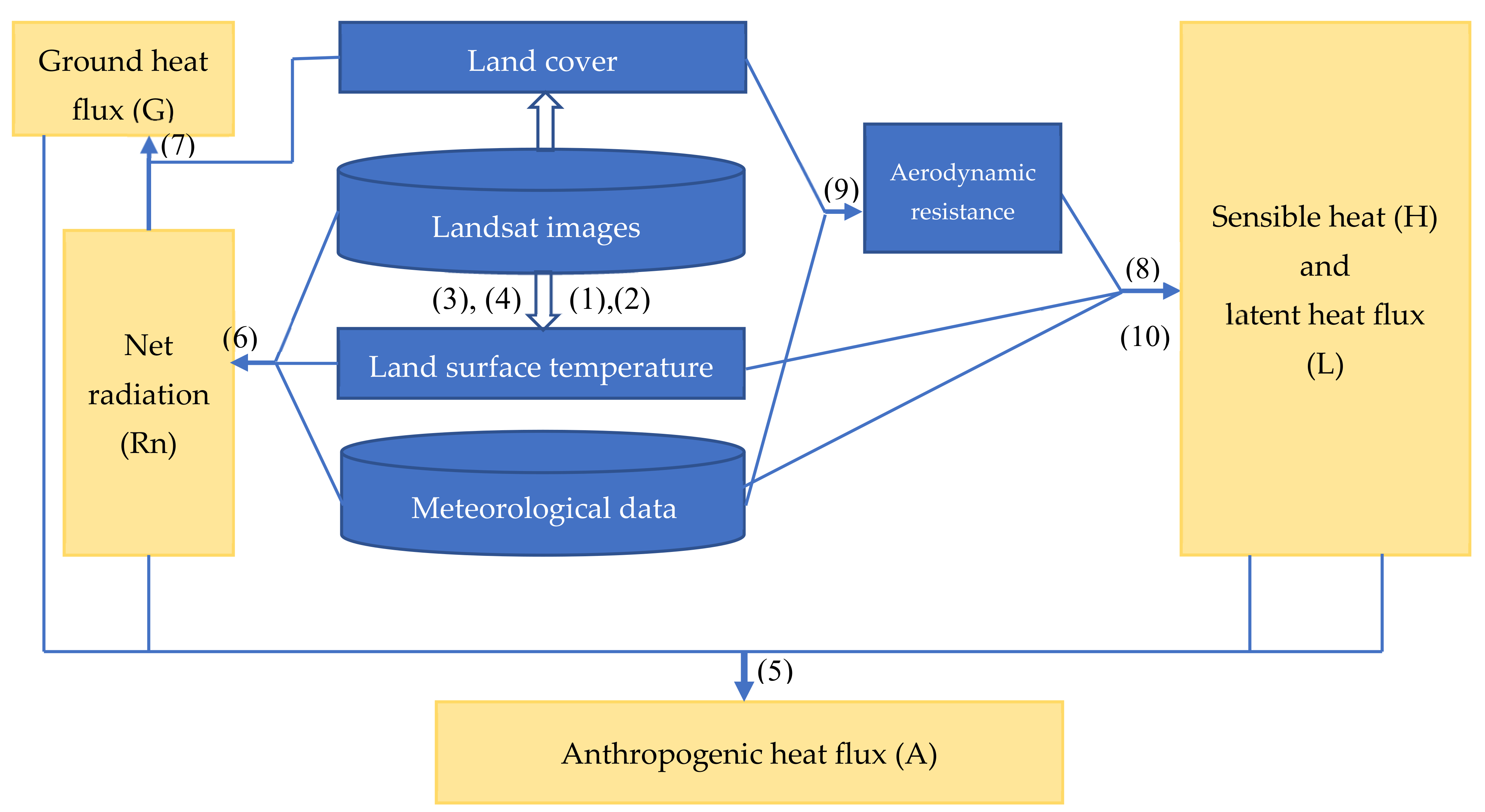
16]. The surface energy balance method, based on remote sensing data and meteorological data, uses empirical formulas to obtain the contribution of net surface radiation, soil heat flux, latent heat flux, and sensible heat flux to the surface energy [17,18]. According to the first law of thermodynamics, it uses the remainder method to estimate anthropogenic heat flux. Compared with the first two methods, the data of remote sensing and meteorological for the surface energy balance method are easy to obtain. The data have the characteristics of high spatial resolution and wide coverage and can be used to determine instantaneous anthropogenic heat flux to study the characteristics of temporal and spatial changes.
The method is based on the surface energy balance and has been applied by previous studies using remote images for research on urban anthropogenic heat. For example, Kato and Yamaguchi used ASTER and ETM+ data to conduct an anthropogenic thermal analysis in Nagoya, Japan, and found that the spatial distribution and seasonal variation trend of anthropogenic heat are consistent with actual energy consumption, which is high in developed areas and low in rural areas, and factories have high annual anthropogenic thermal energy [19]. Zhuo et al. used ASTER data to study the anthropogenic heat and energy consumption of residential and commercial buildings in Indianapolis in the summer, and the results showed that the spatial pattern and scale of anthropogenic heat and building energy consumption are consistent [20]. Wong et al. used HJ-1B data to analyze Hong Kong’s anthropogenic heat based on the surface energy balance method, and the results showed that anthropogenic heat flux is related to building density and building height, and the winter correlation coefficients are 0.94 and 0.62, respectively [21]. Hu et al. used ASTER imagery and meteorological observation data to analyze Beijing’s anthropogenic heat and found that anthropogenic heat is positively correlated with the surface temperature and has a greater impact in the summer [22].
The previous researches mainly focus on quantitatively estimating the intensity of anthropogenic heat based on different scales, analyzing spatiotemporal characteristics, influencing factors, and the impact on the environment. Research on a global scale has shown that the northern mid-latitudes contribute most to the global AHF, and the distribution of anthropogenic heat has the characteristics of regional concentration, mainly concentrated in the areas with high-density population and industries [23,24]. In addition, some studies mapping detailed anthropogenic heat using countries and megacities as research areas [25,26,27] found that the range of anthropogenic heat in China’s large cities is between 60 to 190 W/m2 [28] and that the east has significantly more anthropogenic heat than the west [29]. Factors such as the density and height of buildings, functional urban zones, and impervious surface coverage can affect the intensity of anthropogenic heat [20,30]. There are a lot of studies showing that the change of anthropogenic heat not only causes a variation in urban temperature but also affects the air quality of the city, affecting human health and social and economic development [31,32,33,34]. However, there is a lack of research involving analysis of the temporal and spatial characteristics of anthropogenic heat. The spatial pattern and intensity changes of anthropogenic are the result of multiple factors such as human activities, underlying changes, and economic development. Therefore, exploring the temporal and spatial characteristics of anthropogenic heat can elucidate the impact of human activities and the urban thermal environment.
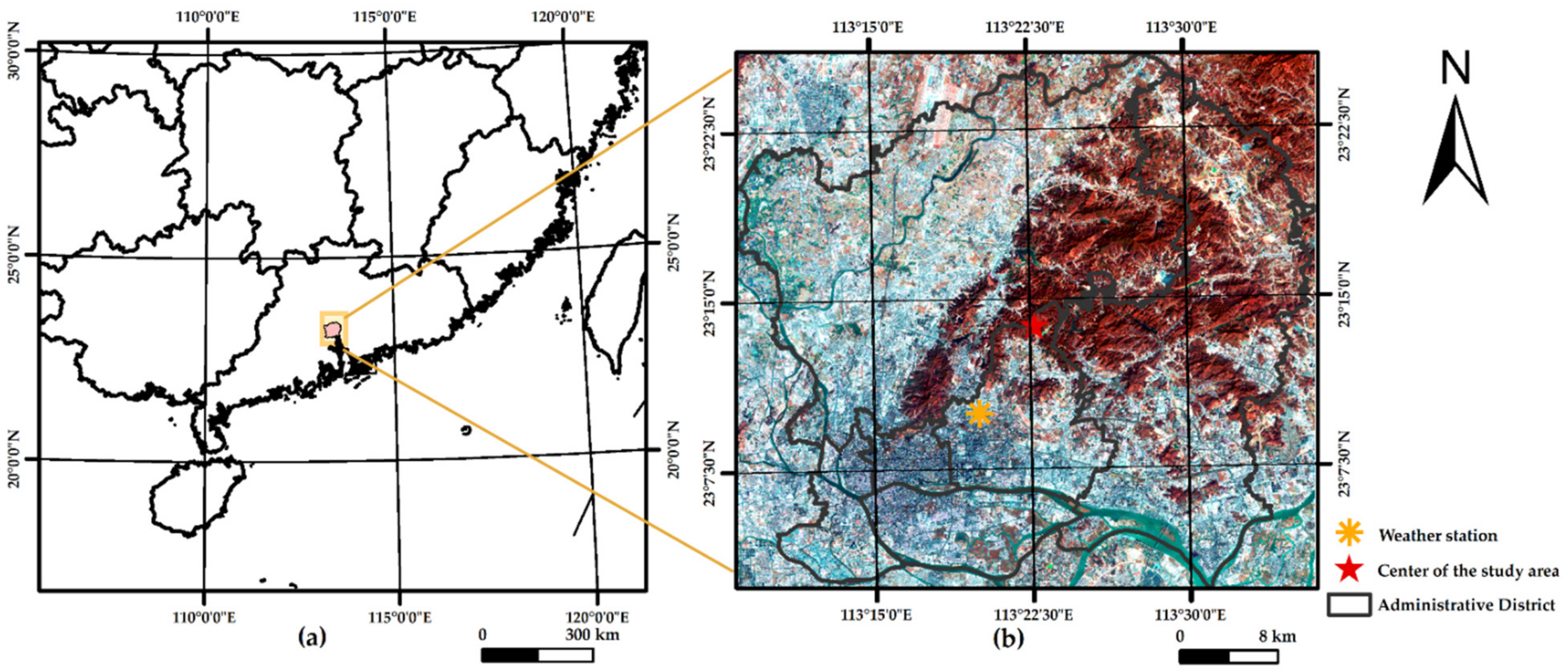
Over the past decades, Guangzhou has been experiencing rapid industrialization and urbanization. As a result, the increased intensity of human activity has stimulated a great increase of energy consumption. Therefore, a time-series analysis of the distribution and evolution and the driving force of urban anthropogenic heat is necessary to evaluate its impact on the thermal environment. In this study, taking the urban area of Guangzhou as an example, based on Landsat time-series image data and the surface energy balance equation, the urban anthropogenic heat for winter from 2004 to 2020 was estimated. The objective of this study was to analyze the spatial distribution and the characteristics of the evolution and explore the evolutionary laws and driving factors of the urban anthropogenic thermal environment.

2. Materials and Methods

2.1. Study Area

Guangzhou is the economic and political center of South China, located in the northern edge of the Pearl River Delta. The study area is the central urban area of Guangzhou (as shown in Figure 1), including 6 districts of Liwan, Yuexiu, Haizhu, Tianhe, Baiyun, and Huangpu, with a range of 113°8′ to 113°36′ E and 23°2′ to 23°25′ N. The topography of the study area is high in the northeast and low in the southwest, and it has a subtropical maritime monsoon climate with an average annual temperature of about 21 °C. It covers an area of approximately 1480 km2 and has a permanent population of approximately 9.67 million in 2019. As a core city in South China, Guangzhou is in a period of rapid economic development, significantly promoting the development of urbanization. The massive increase in urban population and the enhancement of human activities have a huge impact on urban anthropogenic heat, such as the heat island effect, ecological damage, and eco-environmental effects and incipient crises in energy availability.

2.2. Data and Preprocessing

The main data used in this study include remote sensing images and meteorological data. The ancillary data include statistical data of population and gross domestic product (GDP) in 2004, 2009, 2014, and 2020 from the statistical yearbooks, and the distribution map of the urban functional land from Guangzhou Municipal Planning and Natural Resources Bureau.
Remote sensing images include a Landsat 5 TM image (acquired on 21 January 2004 and 2 January 2009) and a Landsat 8 OLI/TRS image (acquired on 16 January 2014 and 18 February 2020), provided by United States Geological Survey (https://earthexplorer.usgs.gov/, accessed on 13 January 2021) and Geospatial Data Cloud Platform of Computer Network Information Center of Chinese Academy of Sciences (http://www.gscloud.cn, accessed on 13 January 2021), the path/row of which is 122/044. The spatial resolution for the sensor of Landsat5 TM and Landsat8 OLI/TRS is 30 m in the short-wave band and 120 m (TM image),100 m (TRS image) in the thermal band. The detailed data are shown in Table 1. The projection of all the images are UTM WGS84. They were preprocessed with radiometric calibration and atmospheric correction by using FLAASH atmospheric correction method based on ENVI 5.3 software.
The land cover classification has been taken by the supervised classification method, which was divided into six types: construction land, forest land, cultivated land, grassland, water body, and bare land. Accuracy assessment is performed by the true land cover types, which is digitized using ArcGIS based on Google Earth image. The overall accuracy of each year is above 90%, and the Kappa coefficient is above 0.8.
The meteorological data came from China Meteorological Data Network (http://data.cma.cn/site/index.html, accessed on 13 January 2021). The selected weather station is Guangzhou Station (23°10′ N, 113°20′ E) and its district station number is 59278. The meteorological data have undergone strict quality control and inspection, which includes atmospheric temperature, vapor pressure, saturated vapor pressure, wind speed, air density, and total solar radiation. The detailed data are shown in Table 2.

2.3. Methods

2.3.1. Inversion of the Land Surface Temperature

The radiative transfer equation method [35] is used to estimate the surface temperature. The algorithm is specifically expressed as:
B T s = L λ L τ 1 ε L τ ε ,
T s = K 2 ln K 1 B T s + 1 ,
where T s is the surface temperature in K, and L λ is the radiance value of the infrared band. ε represents the surface emissivity. τ ,   L , L are the atmospheric transmissivity, the upwelling radiation and downwelling radiation respectively, which can be obtained from NASA (http://atmcorr.gsfc.nasa.gov/, accessed on 13 January 2021). K 1 , K 2 represent the calibration parameter of the infrared band: K 1 =607.76 W∙m−2∙μm−1∙sr-1, and K 2   = 1260.56 K for the band 6 of Landsat TM; K 1   = 774.89W∙m−2∙μm−1∙sr-1 and K 2   = 1321.08 K for the band 8 of Landsat OLI.
The surface emissivity ε is estimated based on the following equation [36] in this study:
ε = 0.004 N D V I N D V I m i n N D V I m a x N D V I m i n + 0.986
N D V I = B N I R B R B N I R + B R
where NDVI is the normalized difference vegetation index, and N D V I m i n and N D V I m a x are the minimum and maximum value, respectively. B N I R and B R represent the near-infrared band and red band of the Landsat images, respectively.

2.3.2. Estimating Anthropogenic Heat Flux based on the Surface Energy Balance Model

Anthropogenic heat flux (AHF) was generally used to represent the intensity of anthropogenic heat. Here, the surface energy balance model [18] was used to calculate AHF, which can be expressed as:
A = G + H + L R n
where R n is the net radiation (W/m2), A is the AHF (W/m2), G is the ground heat flux (W/m2), H is the sensible heat (W/m2), and E is the latent heat flux (W/m2). In the energy balance equation, the net radiation ( R n ) is the sum of solar shortwave radiation and longwave radiation reaching the land surface. It is the net solar radiation energy actually received by the earth’s surface after being reflected by the surface. Rn is determined by parameters such as surface albedo, specific emissivity, and surface temperature. It is calculated as:
R n = 1 α R s + ε ε a σ T a 4 ε σ T s 4
where RS↓ is the downwelling shortwave radiation (W/m2), which can be described as the total solar radiation retrieved from the meteorological data. α and ε represent the surface albedo and the surface emissivity, respectively, and are derived from the remote sensing data [37]. ε a is the atmospheric emissivity, which is estimated using an empirical equation from Kato and Yamaguchi [38]. σ is the Stefan–Boltzmann constant (5.67 × 10⁻⁸W∙K4/m2), and T a represents the atmospheric temperature in K, which can be obtained from meteorological data. T s is the land surface temperature in K, which is estimated based on Equation (2).
The ground heat flux (G) represents the heat exchange energy between the surface and deep layers of the soil. In order to accurately estimate soil heat flux, it is necessary to understand the thermal conductivity of the surface material and the vertical temperature distribution. However, it is difficult to obtain the parameters throughout the study area. There is a linear relationship between soil heat flux and net surface radiation in the existing studies [19,22]. Therefore, it can be estimated from the net surface radiation flux as the following equation:
G = C g R n
where C g is the coefficient, which changes according to factors such as land cover type and season. C g is related to the heat capacity of the surface material and its thermal conductivity. The higher the heat capacity, the lower the C g value. The higher the thermal conductivity, the higher the C g value [19,22,39]. The value of C g in this study is shown in Table 3.
The sensible heat (H) is the energy exchanged between the surface and the atmosphere, characterizing the energy of heating the air. It is estimated based on the following equation:
H = ρ C P T s T a / r a
where ρ is the air density in kg/m3. C P is the specific heat of air at constant pressure (J/kg∙K). r a is the aerodynamic resistance in s/m which is calculated using the following equation:
r a = ln z m d z 0 m ln z h d z 0 h k 2 u z
where z m and z h represent the height of wind and humidity measurement in meters, respectively. d is the zero-plane displacement height in meters. z 0 m is the roughness length governing momentum transfer in meters, and z 0 h is the roughness length governing transfer of heat and vapor in meters. k is the von Karman constant (k = 0.41), and u z is the wind speed in m/s. The values of z 0 m , z 0 h , and d in this study refer to the existing research results, as shown in Table 3 [19,39].
Latent heat flux (L) refers to the heat flux exchanged between the underlying surface and the atmosphere, including surface water evaporation and vegetation transpiration, which is an important part of the water balance. Latent heat flux is always related to parameters such as air density, saturated vapor pressure of the underlying surface, and aerodynamic resistance. Here, we used the formula proposed by Kato [19] to calculate L:
L = ρ C P γ × e s e a r a + r s
where e s is the saturation vapor pressure; e a is air vapor pressure; and γ is the psychrometric constant in hPa/K, which is related to the vapor pressure in the air and the temperature. r a is aerodynamic resistance in s/m, and r s is the stomatal resistance in s/m, which is estimated using the calculation method proposed by Nishida [38,40,41]. ρ and C P have the same meanings as in Equation (8).
The workflow diagram for the overall methodology is shown in Figure 2.

2.3.3. Transition Matrix

In this study, we used the mathematical differences to quantify the changes in anthropogenic heat, which could be demonstrate as:
S A = A 2020 A 2004  
where S A is anthropogenic heat change, and A 2020 and A 2004 are the AHF value of 2020 and 2004, respectively. The S A results could be classified into four categories based on natural breakpoint method: (1) anthropogenic heat drop (AHD), where S A is less than –20 W/m2; (2) anthropogenic heat stable (AHS), where S A is between –20 W/m2 to 20 W/m2; (3) anthropogenic heat increase (AHI), where S A is 20 W/m2 to 60 W/m2; and (4) anthropogenic heat increase sharply (AHIS), where S A is greater than 60 W/m2.
In order to quantitatively explore the magnitude and law of conversion in the anthropogenic heat from 2004 to 2020, the spatial analysis tool was used to establish the transfer matrix of different levels of anthropogenic heat. According to its values, AHF was divided into four types: (1) low-AHF zone, where the value of AHF is 0–100 W/m2; (2) medium-AHF zone, where the value of AHF is 100–200 W/m2; (3) high-AHF zone, where the value of AHF is greater than 200 W/m2; and (4) zero-AHF zone, where the value of AHF is below 0 W/m2.
The general form of the transition matrix is as follows:
S i j = S 11   S 12   S 1 n S 21   S 22   S 2 n       S n 1   S n 2   S n n
where S is the land area of anthropogenic heat; n represents the number of types of anthropogenic heat; i is the anthropogenic heat type at the beginning of the time period; and j is the anthropogenic heat type at the end of the time period. When i = j , S i j represents the unchanged area of the anthropogenic heat type; when i j , S i j represents the area transferred from anthropogenic heat type i to anthropogenic heat type j.2.3.4. Migration of Gravity Center.
The gravity center refers to the point where the forces in various directions can maintain balance in the regional space, which is an important spatial index describing the spatial transformation of geographic elements. The gravity center can reflect the overall heterogeneity of the spatial orientation, and its dynamic migration can reflect the overall migration trajectory of the spatial distribution of geographic elements. We can clearly understand the spatiotemporal evolution pattern in terms of space through researching the shifting of the gravity center [42]. Different anthropogenic heat level types are introduced into the concept of gravity center in this research. The gravity center of anthropogenic heat is the geometric center of the same anthropogenic heat level type in the area, and the gravity center of anthropogenic heat deviates from the geometric center for an uneven distribution of anthropogenic heat in the area, for which the offset direction points to the "high density" location of anthropogenic heat. For multiple geographic objects, the coordinates of the gravity center can be expressed as:
X ¯ = i = 1 n x i n
Y ¯ = i = 1 n y i n
where X ¯ and Y ¯ represent the latitude and longitude coordinates of the gravity center of different types of anthropogenic heat. x i and y i indicate the latitude and longitude coordinates, respectively, of each patch of anthropogenic heat, and n is the number of patches.
The shift distance of the gravity center can be used to express the spatial change characteristics of the feature type, and the expression is as follows:
d = X t + 1 ¯ X t ¯ 2 + Y t + 1 ¯ Y t ¯ 2
where ( X t + 1 ¯ ,   Y t + 1 ¯ ) and ( X t ¯ ,   Y t ¯ ) are the gravity center of elements at different times.

3. Results

3.1. Temporal and Spatial Changes of AHF

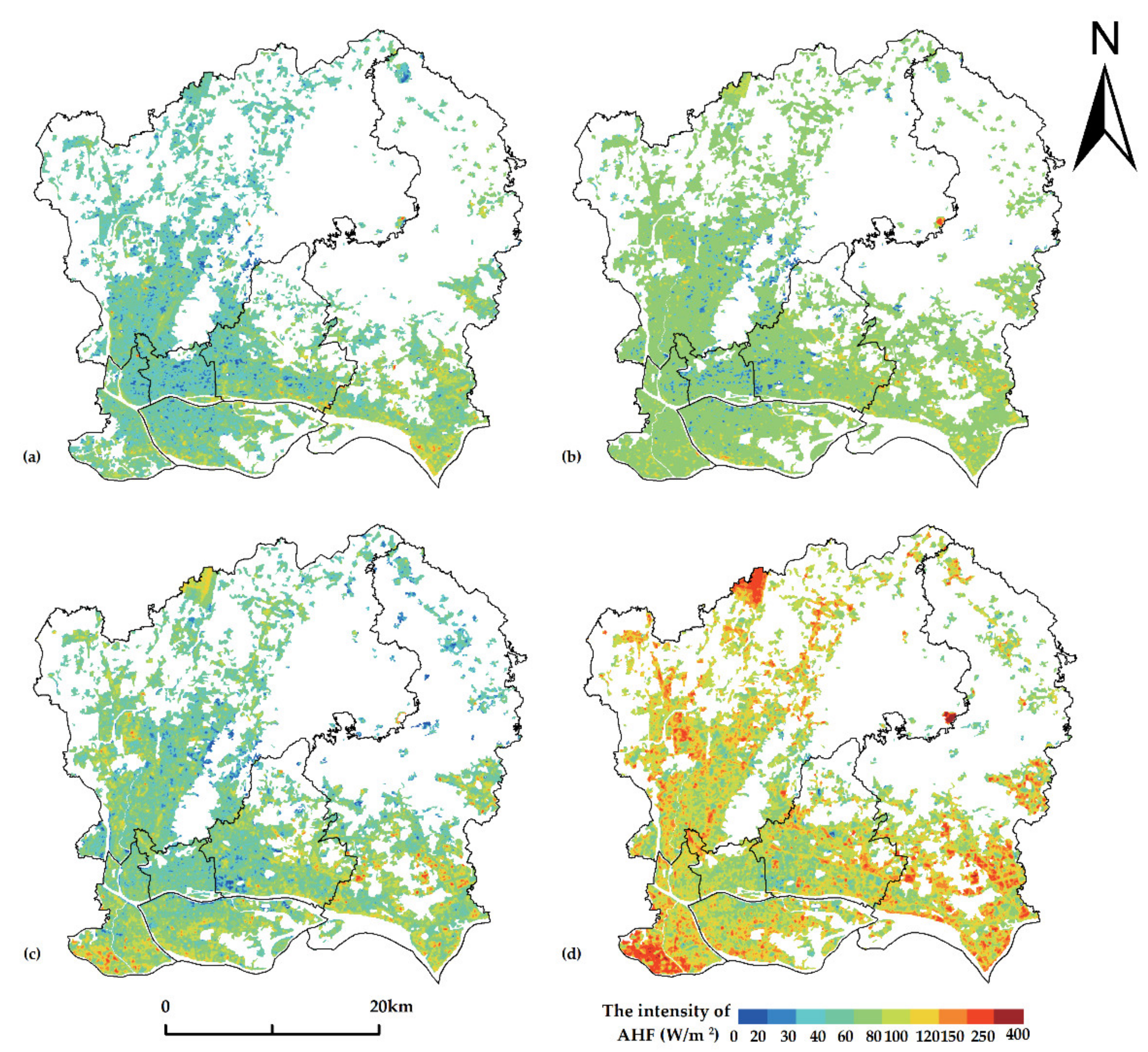
The spatial distribution characteristics of AHF in the central urban area of Guangzhou were obtained and are shown in Figure 3. It is clear from the results that the AHF distribution in the research area changed significantly from 2004 to 2020. The anthropogenic heat expanded rapidly in the space and increased rapidly in terms of value.
The statistics of anthropogenic heat in 2004, 2009, 2014, and 2020 are shown in Table 4. The average value and the main distribution range can reflect the overall level, and the maximum value represents an area of high energy consumption. The main distribution range of the AHF value increased from 32.70 to 90.00 W/m2 in 2004 to 52.70 to 131.60 W/m2 in 2020. The average values of AHF are 53.91, 59.26, 62.26 and 96.28 W/m2, respectively. The maximum AHF in 2004 and 2020 was 245.71 and 397.95 W/m2, respectively. From the perspective of spatial distribution, it is clear that there are obvious spatial differences at different times. Among them, the areas with high AHF in 2004 were mainly distributed along the river and port areas; high AHF areas in 2009 and 2014 were more scattered than that in 2004, moving from the southwest of the central city to the north; there was a large number of AHF peak areas in 2020 in the outer areas of the city.
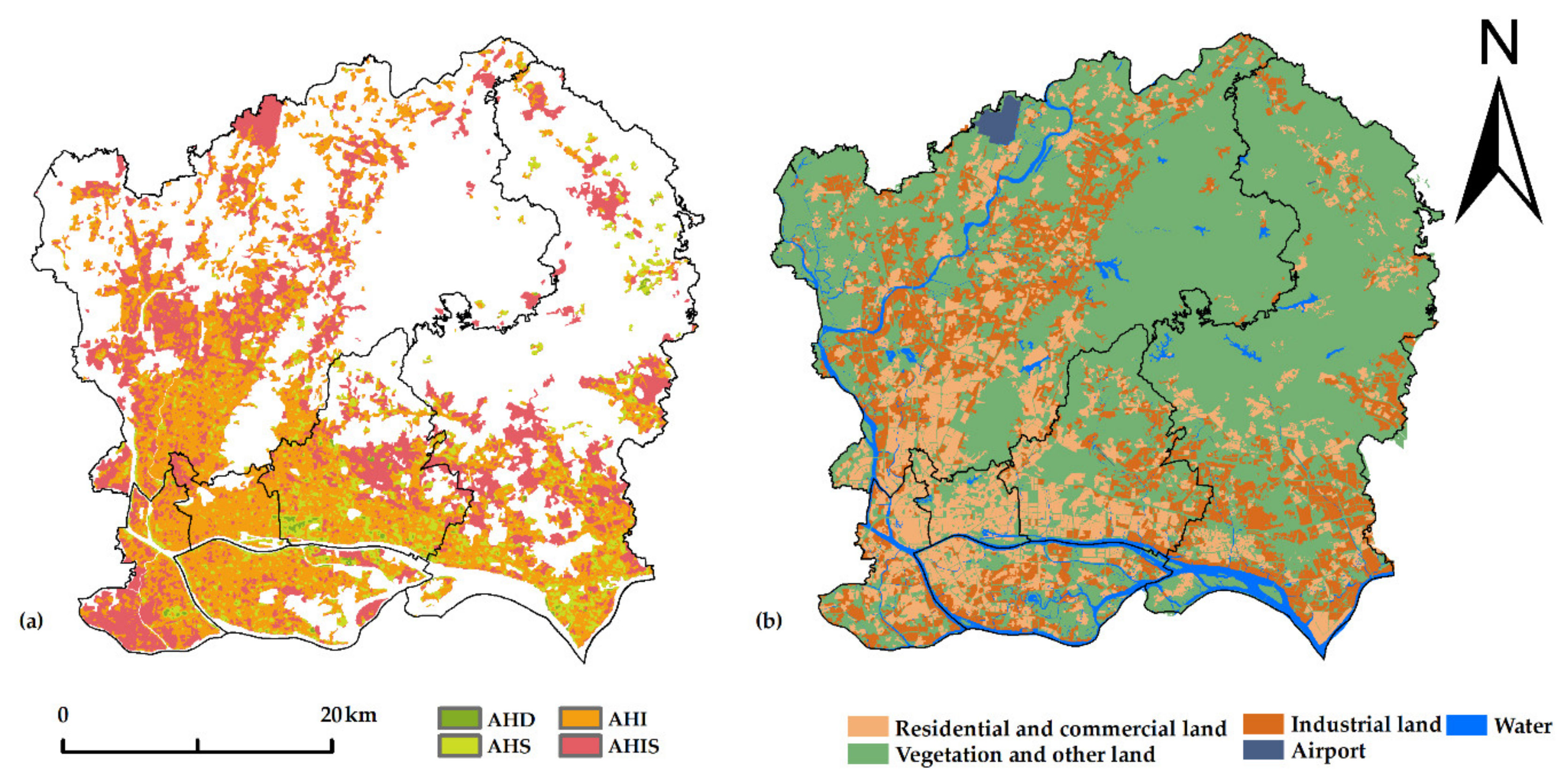
The intensity of anthropogenic heat in 2004 was lower than that in 2020, and the types of anthropogenic heat change are shown in Figure 4a. From the statistics in Table 5, it can be seen that the largest area is the AHI type, with an area of 323.44 km2, accounting for 21.99% of the research area. Next are the AHIS and AHS types, with 231.7 and 77.54 km2, accounting for 15.75% and 5.27%, respectively. The smallest area is the AHD type, with 4.58 km2, accounting for 0.31%.
A comparison was made between the urban functional land and the anthropogenic heat change. The distribution map of the urban functional land in the central city of Guangzhou is shown in Figure 4b. It can be seen that the type of AHI was mainly distributed in the southwest of the center of the study area, and the main functional land types here are residential land and commercial land. The anthropogenic heat in residential and commercial areas mainly comes from electrical energy consumption and human metabolism. There are densely populated and densely built areas in the southwest of the center of the study area, which have been the main reason for a slight increase in anthropogenic heat. The AHIS type was mainly distributed in the outskirts of the central city where the main types of functional land are industrial land and airport land. The anthropogenic heat of industrial land mainly comes from the use of electricity and coal, and frequent air transportation in the airport area causes a lot of waste heat emissions. The new Baiyun International Airport and other transportation facilities have been constantly improving, and their convenient transportation attracted a large number of industrial migration and construction to the mainland [43]. Therefore, the release of a large amount of waste heat because of industrial production and large-scale logistics and transportation made anthropogenic heat rise sharply [39].

3.2. Analysis of the Transition Matrix

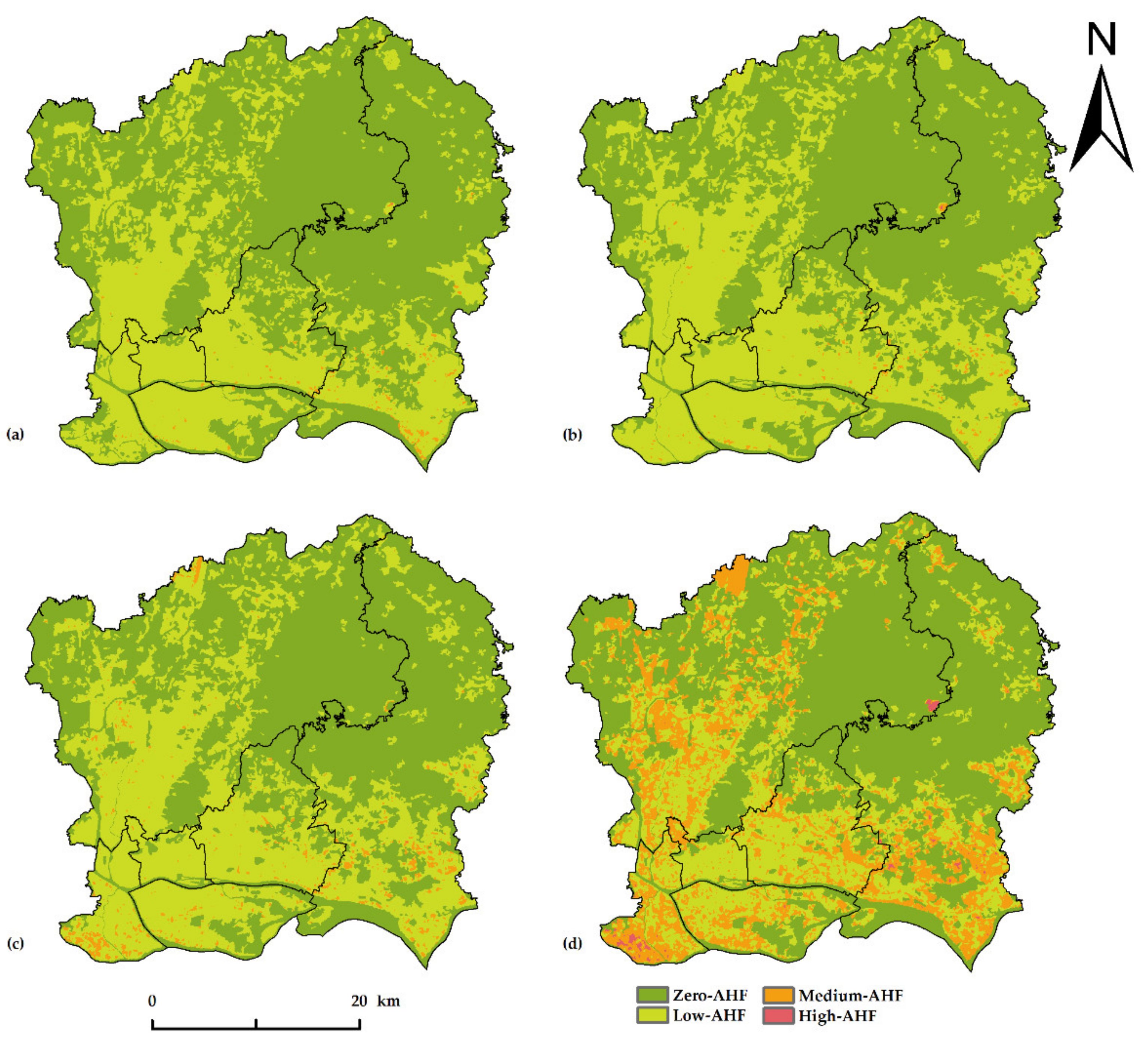
The distribution of different levels of AHF in 2004 and 2020 is shown in Figure 5. It is clear to see that the area of medium-AHF zone expanded significantly, while the area of low-AHF zone shrunk. The area changes of different levels of AHF are shown in Table 6. During the period 2004–2020, the zero-AHF zone and low-AHF zone accounted for the largest area, exceeding 80%. The next is the medium-AHF zone, and the smallest area is the high-AHF zone, with less than 0.3% of the total research area. From the overall dynamic process, it can be seen that the area of the medium-AHF zone and high-AHF zone increased, while the area of the zero-AHF zone and low-AHF zone decreased. During the study period, the zero-AHF zone decreased significantly, which accounted for a decrease from 63.70% to 56.69%, reduced by 103.06 km2, and the period of the fastest decrease was during 2004 to 2009, from 63.70% to 58.86%, with the area decreased by 71.09 km2. For the low-AHF zone, its area increased first and then decreased: during the period 2004 to 2009 and 2009 to 2014, the area of low-AHF zone was increasing steadily, with the proportion increased from 35.85% to 40.86% and the area increased by 73.79 km2. During the period 2014 to 2020, the area of low-AHF decreased significantly, from 40.86% to 26.56%, with the area decreased by 210.41 km2. During the period 2004 to 2020, the proportion of the medium-AHF zone increased significantly, from 0.46% to 16.48%, with the area increased by 235.65 km2, and the fastest growth period was during 2014 to 2020, with the area increased by 213.96 km2. The proportion of the high-AHF zone increased slightly, from 0.001% to 0.28%, with the area increased by 4.05 km2. Therefore, during period of 2004 to 2009 and 2009 to 2014, the transfer-out of the zero-AHF zone and the transfer-in of the low-AHF zone were the main changes, while during the period of 2014 to 2020, The transfer-out of the zero-AHF zone and low-AHF zone and the transfer-in of the medium-AHF zone were the main changes. In all, the level types of AHF in the central urban area from 2004 to 2020 changed extremely significantly, and the overall situation is unbalanced.
According to the transfer matrix (Table 7), the direction and quantity of changes among different level types of AHF could be analyzed. It can be seen that the various level types of AHF were transferred in and out during the period 2004–2020, and the transfer volume between types became more complicated.
The low-AHF zone was the largest of the transferred-out areas, with 217.06 km2, which mainly transferred to the medium-AHF zone. The next was the zero-AHF zone, with an area of 132.19 km2, which mainly converted to the low-AHF zone and medium-AHF zone, with transfer rates of 8.41% and 5.57%, respectively. The smallest transfer-out area was the high-AHF zone, with area only of 0.01 km2.
The largest of the transfer-in areas was the medium-AHF zone, with an area of 237.64 km2, and the main contribution was from the zero-AHF zone and low-AHF zone. The second was the low-AHF zone with an area of 80.43 km2, and the main contribution came from the non-built-up area. The smallest was the high-AHF zone of 4.06 km2.
The absolute number of transfer-in and transfer-out areas of the low-AHF zone was relatively large; thus, the changes in low-AHF were the most intense, while the number of transfer-in and transfer-out areas in the high-AHF zones was small, which indicated that the high-AHF zones were relatively stable.

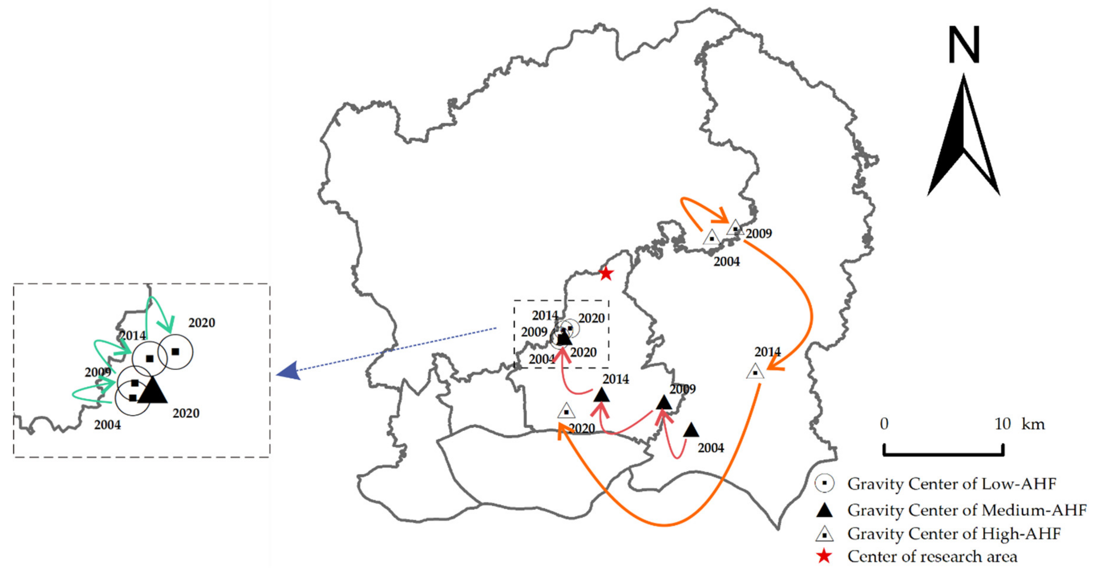
3.3. Spatial Migration of Gravity Center

The gravity center of different levels of AHF in the central urban area of Guangzhou is shown in Figure 6 and can be used to explore the migration trace of different levels of AHF and reveal the temporal and spatial evolution of anthropogenic heat.
This study used the center of the study area as a reference. Spatially, the gravity center of the low-AHF zone moved to the northeast during 2004–2020, but the gravity centers of the low-AHF zone in the four years were all located in the southwest near the center of the study area, which indicated that the distribution of the low-AHF zone was uniform, and the southwest is relatively denser than the northeast. The gravity center of medium-AHF zone migrated to the northwest, from the southeast of the study area, and the gravity centers of medium-AHF zone in the four years were all located in the southern part of the center of the study area. This indicated that the southern part of the medium-AHF zone was denser than the north. The gravity center of the high-AHF zone migrated to the southwest. In 2004 and 2009, the gravity centers of the high-AHF zone were located in the northeast of the study area. And then it migrated to the north, located in the southeast of the center of the study area in 2014, while it was located in the southwest of the center of the study area in 2020.
The migration distances of different levels of AHF are shown in Table 8, which were significantly different. The shortest migration distance was the low-AHF zone with 1.31 km during 2004 to 2020, and its migration distances were 0.32 km in 2004–2009, 0.59 in 2009–2014, 0.55 km in 2014 to 2020, respectively. The next was the medium-AHF zone with 13.19 km, and its migration distances were 3.26 km, 5.3 km, and 5.7 km, respectively. The longest migration distance was the high-AHF zone with 19.06 km, and its migration distances were 2.31 km, 12.2 km, and 16.24 km, respectively. Based on Table 6 and Figure 5, the area and distribution of low-AHF played the main control role in the study area during the period 2004–2020. Therefore, the gravity center of migration distance of the low-AHF zone was relatively short. The medium-AHF was mainly distributed in the southeast of study area in 2004, while the medium-AHF gradually became the main type in 2020, concentrated in the southwest and northwest, and scattered in the north. Therefore, the gravity center of medium-AHF had a large shift. The high-AHF zone had a small change in area but a large change in space. The high-AHF zone was mainly located in the east in 2004. However, it expanded to the north and southeast in 2020. To sum up, the low-AHF zone had relatively stable spatial changes during the period from 2004 to 2020, while the medium-AHF zone and high-AHF zone changed more drastically.

4. Discussion

4.1. Validation of the Estimated Heat Fluxes

The surface heat balance mainly depends on the surface material and local aerodynamic conditions. Since Meteorological parameters vary with location and time, more and accurate spatial meteorological data can reduce the error of anthropogenic heat flux estimation. However, due to the difficulty in obtaining multi-station meteorological data, we only used the data from one meteorological reference station to estimate anthropogenic heat flux. Moreover, there is a lack of anthropogenic heat flux measurement data of the study area. Here, we test the accuracy of heat flux estimated in this study by comparing the results of other studies in the same season (Table 9).
In the previous studies, the ratios of H/Rn and L/Rn varied from 0.08 to 0.46 and from 0.00 to 0.10, respectively [19,38,39,44]. The ratios of H/Rn and L/Rn in the present study are in the range of above studies, varying from 0.1 to 0.19 and from 0.03 to 0.07. The values of H/Rn in this study are similar to the results of Nagoya, Japan in 2004 and Xiamen Island, China in 2009, but lower than the results of Nagoya, Japan in 2000 and Tokyo, Japan in 2002, which is mainly due to the incident solar radiation and the different characteristics of the surface [39]. The values of L/Rn in this study are similar to the results of Tokyo, Japan in 2002, but higher than the results of Nagoya, Japan in 2000 and 2004 and Xiamen Island, China in 2009, which are related to the proportion of impervious surfaces [44]. We also compared the distribution of the mapped AHF in 2009 with the result by using the energy-consumption inventory based on top-down approach in 2010. Both distribution patterns are roughly the same, showing a trend of low AHF value in the central city and high AHF value in the edges in tiny spots [30]. Through the above comparative analysis, it is found that the results of this study are consistent with the results of other existing studies. Therefore, the anthropogenic heat flux estimated is credible to some extent.

4.2. Analysis of Influencing Factors of AHF

From 2004 to 2020, the total population of Guangzhou’s central urban area increased from 3.45 million to 9.67 million, with a net increase of 6.22 million and an increase rate of 389,000 per year. Population is one of the most active factors in the urban structure [45] and has an important impact on AHF. Population data can be used to express the intensity of human activities; thus, the intensity of population activities is more intense in densely populated areas. A correlation analysis between the population data of each district and its AHF in 2004, 2009, 2014, 2020 was carried out to explore the relationship between AHF and population in various districts (Figure 7a). It can be seen that AHF in each district has a positive correlation with the total population (R2 = 0.3046), and correlation is significant at the 0.01 level (two-tailed). As reported by Dong Y et al. [23], on a global scale, the areas accommodating a dense population have a relatively higher values of AHF than the areas with low population density. The increase in the urban population will inevitably be reflected in the strengthening of urban residents’ demand for housing, transportation, and public facilities [46]. Therefore, the urban population can most directly affect anthropogenic heat, and the increase in the total population will lead to an increase in the intensity of anthropogenic heat.
In 2004, the total GDP of the central urban area of Guangzhou was 213.65 billion RMB. It grew to 1693.78 billion RMB by 2020, with a growth rate of 92.502 billion RMB/a. Here, we also used the GDP of each district and its AHF in 2004, 2009, 2014, 2020 to take a correlation analysis (Figure 7b). It can be seen that the intensity of AHF in each district has an obvious linear relationship with the total GDP of districts (R2 = 0.3425), and correlation is significant at the 0.01 level (two-tailed). Previous studies have also found that the mid-latitudes of the northern hemisphere contribute the main global anthropogenic heat [23]. Countries with high GDP are mainly distributed in this region, such as the United States, China, Japan, Germany, and the United Kingdom. There is a big difference in anthropogenic heat between east and west in China [29], and space distribution of China’s anthropogenic heat is similar to economic distribution characteristics, especially in some economically developed large cities, in which the intensity of anthropogenic heat is significantly higher than that in nearby areas [47]. The development of the economy and increased income has also stimulated the emission of anthropogenic heat from residential areas and industrial production activities.
In Figure 4b, the total area of industrial land in the central urban area of Guangzhou was 262.30 km2 in 2020, and it accounts for 17.83% of the study area. An 8 × 8 grid covering the study area was established by ArcGIS, and the proportion of industrial land and the average AHF value in each grid were used to analyze the correlation relationship between the AHF and industrial land in this study (Figure 7c). It can be seen that AHF of each grid is linearly related to the proportion of industrial land area (R2 = 0.4273), and correlation is significant at the 0.01 level (two-tailed). It indicates that the industrial land has a positive influence on AHF, and AHF increases as the area of industrial land increases. Previous studies showed that more than 70.0% of anthropogenic heat emissions in Mainland China come from industrial production [29], and the anthropogenic heat is estimated to have spatial heterogeneity [15]. The distribution of industrial land could contribute to the distribution of anthropogenic heat, and the type and density of industrial land have an influence on the intensity of anthropogenic heat.

4.3. Limitations

The anthropogenic heat was effectively estimated based on the energy balance model. However, there are some limitations in this study. First, February 2020 was in a period of the COVID-19 pandemic when human activity and production had been limited. AHF is affected by human activities. Therefore, the estimation of the anthropogenic heat in 2020 may be lower than expected due to the influence of the COVID-19 pandemic. Second, the aerodynamic parameters used in this study are empirical values from previous studies [19,39]. However, the aerodynamic parameters vary with location and time, which makes the experimental results have certain limitations. A more accurate estimation of anthropogenic heat would be obtained if the spatial interpolation of aerodynamic parameters can be realized in real time. Moreover, the spatial pattern of the estimated anthropogenic heat lacks some detail contrasts with multiple publicly datasets, which might be a method of verifying the estimated anthropogenic heat. Validation of the estimated heat fluxes would be more comprehensive if the we can be further validated with existing publicly available anthropogenic heat datasets [48,49].

5. Conclusions

In this study, the central urban area of Guangzhou City was taken as an example to estimate the temporal and spatial variation of anthropogenic heat in different urbanization periods. The energy balance model was used based on remote sensing images. The transfer matrix and the migration of the gravity center was used to analyze the change characteristics of the anthropogenic heat and the drivers of anthropogenic heat change from population, GDP, and industry aspects were also explored. The main conclusions are as follows:
The overall change trend of anthropogenic heat in the central urban area of Guangzhou was enhanced during the period from 2004 to 2020, and the degree of its enhancement was related to the types of urban functional land. The central area of Guangzhou is in a stage of rapid urbanization, which has stimulated a substantial increase in energy demand and supply, and the intensity of anthropogenic heat has also increased. The increase in the intensity of anthropogenic heat in industrial areas and airport areas is greater than that of commercial and residential areas.
There are obvious differences both in area and space for different types of anthropogenic heat with urban development. In terms of area expansion, the areas of the zero-AHF zone, low-AHF zone, and medium-AHF zone changed drastically, with the zero-AHF zone and low-AHF zone transferring out and medium-AHF zone transferring in as the main form, while the area change of the high-AHF zone was relatively stable. The urbanization of Guangzhou’s central urban area has led to an increase in the demand for urban energy consumption, which is also the main reason for the unbalanced state of the single conversion of anthropogenic heat from low-AHF areas to high-AHF areas. Spatially, the distance change of the low-AHF zone is relatively stable; the migration distance is 1.31 km2. The distance changes of the medium-AHF zone and the high-AHF zone are more intense, with migration distances of 13.19 and 19.06 km, respectively. Some large-scale industrial areas were identified in the study area in 2020 with the improvement of transportation equipment, while industrial areas were mainly distributed in port areas in 2004. This is the main reason for the large changes of space in the medium- and high-AHF areas.
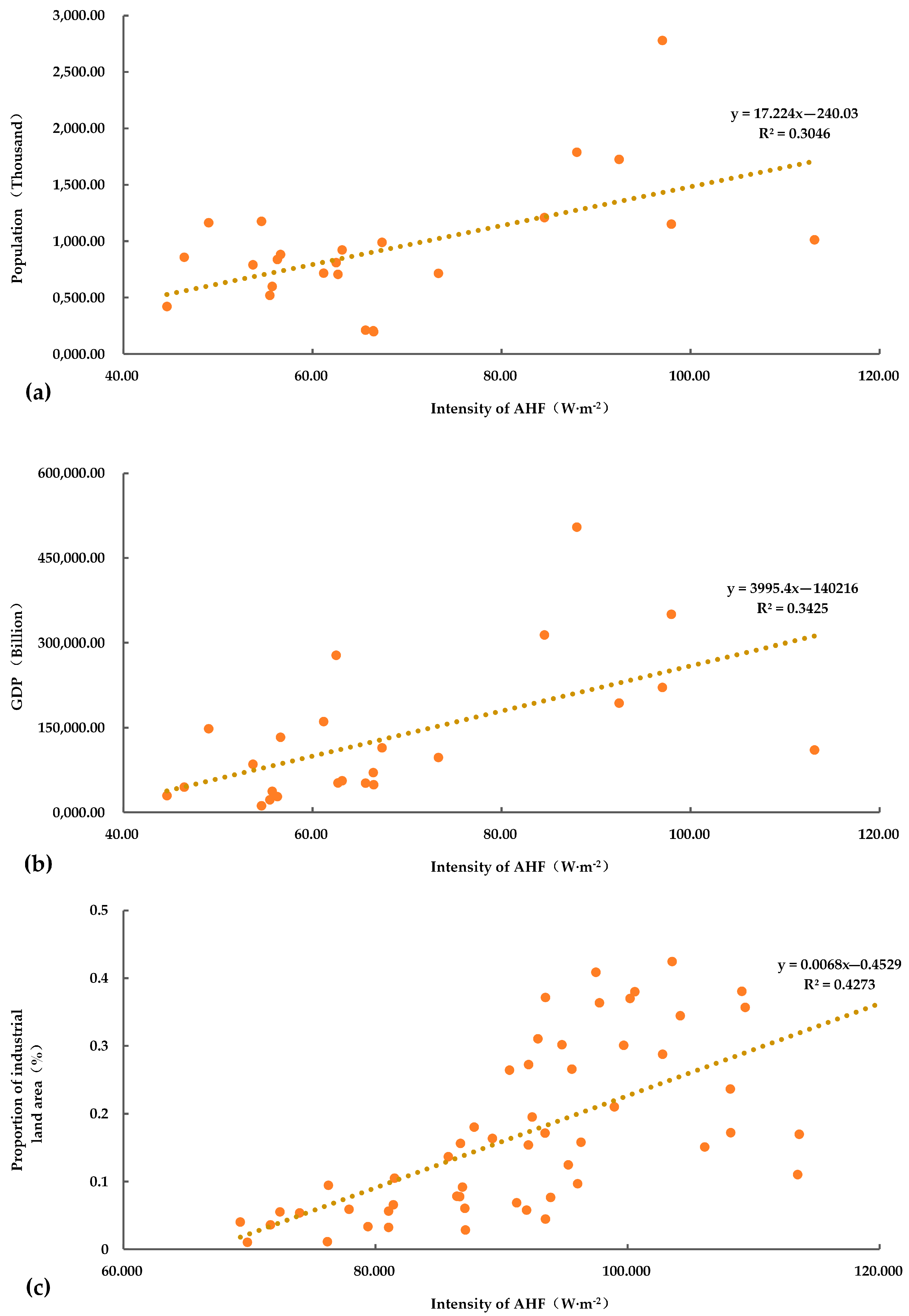
The expansion and enhancement of the influence of human activities, such as the increase in urban population, rapid economic development, and increased industrial production activities, have stimulated the emission of anthropogenic heat, which contributes to the positive impact on the intensity of anthropogenic heat and the occurrence of significant urban anthropogenic heat change. Analysis of the characteristics of temporal and spatial changes in anthropogenic heat and studies on the laws and influencing factors of anthropogenic heat changes will provide references for urban planning and construction in mitigating urban heat islands.

Author Contributions

Conceptualization, Caige Sun and Fenglei Fan; methodology, Caige Sun; investigation and resources, Ting Peng; data curation, Shanshan Feng; writing—original draft preparation, Ting Peng and Caige Sun; writing—review and editing, Yongdong Zhang and Fenglei Fan; visualization, Ting Peng; supervision, Fenglei Fan; project administration and funding acquisition, Caige Sun and Fenglei Fan. All authors have read and agreed to the published version of the manuscript.

Funding

This research was funded by Guangdong Basic and Applied Basic Research Foundation (Grant No.2020A1515010562), the National Nature Science Foundation of China (Grant No. 41901347), and the China Postdoctoral Science Foundation (Grant No.2018M643109).

Data Availability Statement

The data presented in this study are available from author upon reasonable request.

Acknowledgments

We sincerely thank the reviewers for their helpful comments and suggestions about our manuscript.

Conflicts of Interest

The authors declare no conflict of interest.

References

  1. Deng, J.S.; Wang, K.; Hong, Y.; Qi, J.G. Spatio-temporal dynamics and evolution of land use change and landscape pattern in response to rapid urbanization. Landsc. Urban Plan. 2009, 92, 187–198. [Google Scholar] [CrossRef]
  2. Zhou, Q. A review of sustainable urban drainage systems considering the climate change and urbanization impacts. Water 2014, 6, 976–992. [Google Scholar] [CrossRef]
  3. Santamouris, M.; Cartalis, C.; Synnefa, A.; Kolokotsa, D. On the impact of urban heat island and global warming on the power demand and electricity consumption of buildings—A review. Energy Build. 2015, 98, 119–124. [Google Scholar] [CrossRef]
  4. Voogt, J.A.; Oke, T.R. Thermal remote sensing of urban climates. Remote Sens. Environ. 2003, 86, 370–384. [Google Scholar] [CrossRef]
  5. Kikegawa, Y.; Genchi, Y.; Kondo, H.; Hanaki, K. Impacts of city-block-scale countermeasures against urban heat-island phenomena upon a building’s energy-consumption for air-conditioning. Appl. Energy 2006, 83, 649–668. [Google Scholar] [CrossRef]
  6. Ichinose, T.; Shimodozono, K.; Hanaki, K. Impact of anthropogenic heat on urban climate in Tokyo. Atmos. Environ. 1999, 33, 3897–3909. [Google Scholar] [CrossRef]
  7. Sailor, D.J.; Georgescu, M.; Milne, J.M.; Hart, M.A. Development of a national anthropogenic heating database with an extrapolation for international cities. Atmos. Environ. 2015, 118, 7–18. [Google Scholar] [CrossRef] [Green Version]
  8. Chen, S.; Hu, D. Parameterizing anthropogenic heat flux with an energy-consumption inventory and multi-source remote sensing data. Remote Sens. 2017, 9, 1165. [Google Scholar] [CrossRef] [Green Version]
  9. Pigeon, G.; Legain, D.; Durand, P.; Masson, V. Anthropogenic heat release in an old European agglomeration (Toulouse, France). Int. J. Climatol. 2007, 27, 1969–1981. [Google Scholar] [CrossRef]
  10. Oke, T.; Cleugh, H. Urban heat storage derived as energy balance residuals. Bound. Layer Meteorol. 1987, 39, 233–245. [Google Scholar] [CrossRef]
  11. Block, A.; Keuler, K.; Schaller, E. Impacts of anthropogenic heat on regional climate patterns. Geophys. Res. Lett. 2004, 31. [Google Scholar] [CrossRef]
  12. Sailor, D.J. A review of methods for estimating anthropogenic heat and moisture emissions in the urban environment. Int. J. Climatol. 2011, 31, 189–199. [Google Scholar] [CrossRef]
  13. Lee, S.-H.; Song, C.-K.; Baik, J.-J.; Park, S.-U. Estimation of anthropogenic heat emission in the Gyeong-In region of Korea. Theor. Appl. Clim. 2009, 96, 291–303. [Google Scholar] [CrossRef]
  14. Chow, W.T.; Salamanca, F.; Georgescu, M.; Mahalov, A.; Milne, J.M.; Ruddell, B.L. A multi-method and multi-scale approach for estimating city-wide anthropogenic heat fluxes. Atmos. Environ. 2014, 99, 64–76. [Google Scholar] [CrossRef] [Green Version]
  15. Wang, S.; Hu, D.; Yu, C.; Chen, S.; Di, Y. Mapping China’s time-series anthropogenic heat flux with inventory method and multi-source remotely sensed data. Sci. Total Environ. 2020, 139457. [Google Scholar] [CrossRef] [PubMed]
  16. Heiple, S.; Sailor, D.J. Using building energy simulation and geospatial modeling techniques to determine high resolution building sector energy consumption profiles. Energy Build. 2008, 40, 1426–1436. [Google Scholar] [CrossRef] [Green Version]
  17. Christen, A.; Vogt, R. Energy and radiation balance of a central European city. Int. J. Climatol. 2004, 24, 1395–1421. [Google Scholar] [CrossRef]
  18. Oke, T.R. The urban energy balance. Prog. Phys. Geogr. 1988, 12, 471–508. [Google Scholar] [CrossRef]
  19. Kato, S.; Yamaguchi, Y. Analysis of urban heat-island effect using ASTER and ETM+ Data: Separation of anthropogenic heat discharge and natural heat radiation from sensible heat flux. Remote Sens. Environ. 2005, 99, 44–54. [Google Scholar] [CrossRef]
  20. Zhou, Y.; Weng, Q.; Gurney, K.R.; Shuai, Y.; Hu, X. Estimation of the relationship between remotely sensed anthropogenic heat discharge and building energy use. Isprs J. Photogramm. Remote Sens. 2012, 67, 65–72. [Google Scholar] [CrossRef] [Green Version]
  21. Wong, M.S.; Yang, J.; Nichol, J.; Weng, Q.; Menenti, M.; Chan, P.W. Modeling of anthropogenic heat flux using HJ-1B Chinese small satellite image: A study of heterogeneous urbanized areas in Hong Kong. IEEE Geosci. Remote Sens. Lett. 2015, 12, 1466–1470. [Google Scholar] [CrossRef]
  22. Hu, D.; Yang, L.; Zhou, J.; Deng, L. Estimation of urban energy heat flux and anthropogenic heat discharge using aster image and meteorological data: Case study in Beijing metropolitan area. J. Appl. Remote Sens. 2012, 6, 063559. [Google Scholar] [CrossRef]
  23. Dong, Y.; Varquez, A.; Kanda, M. Global anthropogenic heat flux database with high spatial resolution. Atmos. Environ. 2017, 150, 276–294. [Google Scholar] [CrossRef]
  24. Chen, B.; Wu, C.; Liu, X.; Chen, L.; Wu, J.; Yang, H.; Luo, T.; Wu, X.; Jiang, Y.; Jiang, L. Seasonal climatic effects and feedbacks of anthropogenic heat release due to global energy consumption with CAM5. Climate Dyn. 2019, 52, 6377–6390. [Google Scholar] [CrossRef]
  25. Smith, C.; Lindley, S.; Levermore, G. Estimating spatial and temporal patterns of urban anthropogenic heat fluxes for UK cities: The case of Manchester. Theor. Appl. Clim. 2009, 98, 19–35. [Google Scholar] [CrossRef]
  26. ICHINOSE, T.; HANAKI, K.; MATSUO, T. Analyses on geographical distribution of urban anthropogenic heat based on very precise geographical information. Environ. Eng. Res. 1994, 31, 263–273. [Google Scholar]
  27. He, C.; Zhou, L.; Yao, Y.; Ma, W.; Kinney, P.L. Estimating temporal-spatial effects of anthropogenic heat emissions upon the urban thermal environment in an urban agglomeration area in East China. Sustain. Cities Soc. 2020, 102046. [Google Scholar] [CrossRef]
  28. Chen, Q.; Yang, X.; Ouyang, Z.; Zhao, N.; Jiang, Q.; Ye, T.; Qi, J.; Yue, W. Estimation of anthropogenic heat emissions in China using Cubist with points-of-interest and multisource remote sensing data. Environ. Pollut. 2020, 266, 115183. [Google Scholar] [CrossRef] [PubMed]
  29. Lu, Y.; Wang, Q.g.; Zhang, Y.; Sun, P.; Qian, Y. An estimate of anthropogenic heat emissions in China. Int. J. Clim. 2016, 36, 1134–1142. [Google Scholar] [CrossRef] [Green Version]
  30. Cao, Z.; Wu, Z.; Liu, L.; Chen, Y.; Zou, Y. Assessing the relationship between anthropogenic heat release warming and building characteristics in Guangzhou: A sustainable development perspective. Sci. Total Environ. 2019, 695, 133759. [Google Scholar] [CrossRef] [PubMed]
  31. Flanner, M.G. Integrating anthropogenic heat flux with global climate models. Geophys. Res. Lett. 2009, 36, 36. [Google Scholar] [CrossRef] [Green Version]
  32. Sailor, D.J.; Lu, L. A top–down methodology for developing diurnal and seasonal anthropogenic heating profiles for urban areas. Atmos. Environ. 2004, 38, 2737–2748. [Google Scholar] [CrossRef]
  33. Schwarz, N.; Schlink, U.; Franck, U.; Großmann, K. Relationship of land surface and air temperatures and its implications for quantifying urban heat island indicators—An application for the city of Leipzig (Germany). Ecol. Indic. 2012, 18, 693–704. [Google Scholar] [CrossRef]
  34. Connors, J.P.; Galletti, C.S.; Chow, W.T. Landscape configuration and urban heat island effects: Assessing the relationship between landscape characteristics and land surface temperature in Phoenix, Arizona. Landsc. Ecol. 2013, 28, 271–283. [Google Scholar] [CrossRef]
  35. Sobrino, J.A.; Jiménez-Muñoz, J.C.; Paolini, L. Land surface temperature retrieval from LANDSAT TM 5. Remote. Sens. Environ. 2004, 90, 434–440. [Google Scholar] [CrossRef]
  36. Gu, J.; Pei, L. Retrieval of Chlorophyll Content and Temperature in Taihu Based on Landsat 8-OLI/TIRS and HJ-1B. Geomat. Spat. Inf. Technol. 2017, 40, 146–151, 156. (In Chinese) [Google Scholar]
  37. Liang, S. Narrowband to broadband conversions of land surface albedo I: Algorithms. Remote Sens. Environ. 2001, 76, 213–238. [Google Scholar] [CrossRef]
  38. Kato, S.; Yamaguchi, Y. Estimation of storage heat flux in an urban area using ASTER data. Remote Sens. Environ. 2007, 110, 1–17. [Google Scholar] [CrossRef]
  39. Liu, J.; Zhao, X.; Lin, J. Analysis of anthropogenic heat discharge of urban functional regions based on surface energy balance in Xiamen Island. J. Geo-Inf. Sci. 2018, 20, 1026–1036. (In Chinese) [Google Scholar] [CrossRef]
  40. Kelliher, F.M.; Leuning, R.; Raupach, M.; Schulze, E.-D. Maximum conductances for evaporation from global vegetation types. Agric. For. Meteorol. 1995, 73, 1–16. [Google Scholar] [CrossRef]
  41. Noilhan, J.a.; Lacarrere, P. GCM grid-scale evaporation from mesoscale modeling. J. Clim. 1995, 8, 206–223. [Google Scholar] [CrossRef] [Green Version]
  42. Fan, F.; Fan, W. Understanding spatial-temporal urban expansion pattern (1990–2009) using impervious surface data and landscape indexes: A case study in Guangzhou (China). J. Appl. Remote. Sens. 2014, 8, 083609. [Google Scholar] [CrossRef] [Green Version]
  43. Xu, J.; Zhao, Y.; Zhong, K.; Zhang, F.; Liu, X.; Sun, C. Measuring spatio-temporal dynamics of impervious surface in Guangzhou, China, from 1988 to 2015, using time-series Landsat imagery. Sci. Total Environ. 2018, 627, 264–281. [Google Scholar] [CrossRef] [PubMed]
  44. Liu, Y.; Shintaro, G.; Zhuang, D.; Kuang, W. Urban surface heat fluxes infrared remote sensing inversion and their relationship with land use types. J. Geogr. Sci. 2012, 22, 699–715. [Google Scholar] [CrossRef]
  45. Yao, Y.; Liu, X.; Li, X.; Zhang, J.; Liang, Z.; Mai, K.; Zhang, Y. Mapping fine-scale population distributions at the building level by integrating multisource geospatial big data. Int. J. Geogr. Inf. Sci. 2017, 31, 1220–1244. [Google Scholar] [CrossRef]
  46. Li, L.; Sato, Y.; Zhu, H. Simulating spatial urban expansion based on a physical process. Landsc. Urban Plan. 2003, 64, 67–76. [Google Scholar] [CrossRef]
  47. Xie, M.; Zhu, G.; Wang, T.; Feng, W.; Zhu, X.; Chen, F.; Ouyang, Y.; Liu, Z. Study on the distribution of anthropogenic heat flux over China. China Environ. Sci. 2015, 35, 728–734. (In Chinese) [Google Scholar]
  48. Varquez, A.C.G.; Kiyomoto, S.; Khanh, D.N.; Kanda, M. Global 1-km present and future hourly anthropogenic heat flux. Sci. Data 2021, 8, 64. [Google Scholar] [CrossRef]
  49. Jin, K.; Wang, F.; Chen, D.; Liu, H.; Ding, W.; Shi, S. A new global gridded anthropogenic heat flux dataset with high spatial resolution and long-term time series. Sci. Data 2019, 6, 139. [Google Scholar] [CrossRef] [PubMed]
Figure 1. (a) Location of the study area in China; (b) study area of the Landsat 8 OLI image (2020-02-18) based on the combination of band5, band4, band3.
Ijgi 10 00160 g001
Figure 2. Workflow diagram for the methodology used to estimate anthropogenic heat flux.
Ijgi 10 00160 g002
Figure 3. Spatial distribution of anthropogenic heat flux (AHF) (a) in 2004, (b) in 2009, (c) in 2014, and (d) in 2020.
Ijgi 10 00160 g003
Figure 4. (a) Types of anthropogenic heat change from 2004 to 2020 and (b) distribution of functional lands.
Ijgi 10 00160 g004
Figure 5. Distribution of anthropogenic heat level types (a) in 2004, (b) in 2009, (c) in 2014, and (d) in 2020.
Ijgi 10 00160 g005
Figure 6. Migration of gravity center of different anthropogenic heat level types.
Ijgi 10 00160 g006
Figure 7. Fitting functions of anthropogenic heat emission intensity with (a) population, (b) GDP, and (c) proportion of industrial land.
Ijgi 10 00160 g007
Table 1. Remote sensing data used in this study.
PathRowSatelliteSensorDateSpatial ResolutionCloud-Cover (%)
122044Landsat5TM2004/1/2130 m (multispectral)
120 (infrared)
2.64
2009/1/20.49
122044Landsat8OLI/TRS2014/1/1630 m (multispectral)
100 m (infrared)
1.62
2020/2/180.05
Table 2. Meteorological data of Guangzhou.
DateMeteorological Data
Atmospheric Temperature (°C)Vapor Pressure (hPa)Saturated Vapor Pressure (F)Wind Speed (m/s)Air Density
(kg/m3)
Total Solar Radiation (W/m2)
2004/1/217.06.012.254.11.248896
2009/1/211.84.617.012.71.226681
2014/1/169.48.119.324.91.217863
2020/2/1810.76.919.324.91.201863
Table 3. Parameters used in this study.
ParameterCultivated LandForest LandGrasslandWaterConstruction LandBare Soil
C g 0.30.130.30.90.20.3
z 0 m (m)0.10.30.10.330.000030.001
z 0 h (m)0.0010.00030.0010.00330.0000880.00002
d (m)0.11.50.10.051.660.05
Table 4. Statistics of anthropogenic heat in the study area.
DateAverage Value (W/m2)Main Distribution Range (W/m2)Max Value (W/m2)
2004-01-2153.9132.70–90.00245.71
2009-01-0259.2633.30–97.20245.5
2014-01-1662.2630.10–105.20228.90
2020-02-1896.2852.70–131.60397.95
Table 5. Statistics of different change types of anthropogenic heat from 2004 to 2020.
TypeAHDAHSAHIAHIS
Area (km2)4.5877.54323.44231.7
Percentage (%)0.315.2721.9915.75
Table 6. Statistics of different levels of anthropogenic heat.
Type2004200920142020Area Change from 2004 to 2020 (km2)
Area (km2)Percentage (%)Area (km2)Percentage (%)Area (km2)Percentage (%)Area (km2)Percentage (%)
Zero-AHF zone936.9963.70%865.958.86%838.9357.03%833.9356.69%−103.06
Low-AHF zone527.335.85%597.3640.61%601.0940.86%390.6826.56%−136.62
Medium-AHF zone6.720.46%7.70.52%28.411.93%242.3716.48%235.65
High-AHF zone0.020.00%0.080.01%2.610.18%4.070.28%4.05
Table 7. Transfer matrix of different anthropogenic heat level types from 2004 to 2020.
Type2020Total 2004
Zero-AHF ZoneLow-AHF ZoneMedium-AHF ZoneHigh-AHF Zone
2004Zero-AHF zoneArea (km2)804.8078.8052.221.16936.99
Percentage in 2004 (%)85.898.415.570.12100
Percentage in 2020 (%)96.5120.1721.5528.58
Low-AHF zoneArea (km2)28.94310.26185.412.72527.30
Percentage in 2004 (%)5.4958.8435.160.52100
Percentage in 2020 (%)3.4779.4176.5066.81
Medium-AHF zoneArea (km2)0.21.634.740.186.72
Percentage in 2004 (%)2.9324.1570.292.63100
Percentage in 2020 (%)0.020.421.954.34
High-AHF zoneArea (km2)0.000.000.010.010.02
Percentage in 2004 (%)0.006.0638.9754.97100
Percentage in 2020 (%)0.000.000.000.27
Total percentage in 2020 (%)100100100100
Total 2020 (km2)833.93390.68242.374.071471.04
Table 8. Migration distances of different anthropogenic heat level types.
TypeMigration Distance (km)
2004–20092009–20142014–20202004–2020
Low-AHF0.320.590.551.31
Medium-AHF3.265.35.713.19
High-AHF2.3112.216.2419.06
Table 9. Heat fluxes ratios to net radiation between the present study and previous studies [19,38,39,44].
Study AreaDataH/RnL/Rn
Present studyGuangzhou, China2004/1/210.160.03
2009/1/20.190.09
2014/1/160.100.08
2020/2/180.110.07
Kato et al. (2005)Nagoya, Japan2000/12/80.460.02
Moriwaki et al. (2004)Tokyo, Japan2002/1/-0.360.10
2002/2/-0.40.07
Kato et al. (2007)Nagoya, Japan2004/2/20.080.00
Liu et al. (2018)Xiamen Island, China2009/3/180.250.01
Publisher’s Note: MDPI stays neutral with regard to jurisdictional claims in published maps and institutional affiliations.

