Article

The Spatiotemporal Interaction Effect of COVID-19 Transmission in the United States

1
Department of Urban Planning, School of Urban Design, Wuhan University, Wuhan 430072, China
2
Center for Geographic Analysis, Harvard University, Cambridge, MA 02138, USA
3
China Data Institute, Ann Arbor, MI 48108, USA
4
Department of Graphics and Digital Technology, School of Urban Design, Wuhan University, Wuhan 430072, China
*
Author to whom correspondence should be addressed.
ISPRS Int. J. Geo-Inf. 2021, 10(6), 387; https://0-doi-org.brum.beds.ac.uk/10.3390/ijgi10060387
Submission received: 24 March 2021 / Revised: 27 May 2021 / Accepted: 3 June 2021 / Published: 4 June 2021

Abstract

:
(1) Background: Human mobility between geographic units is an important way in which COVID-19 is spread across regions. Due to the pressure of epidemic control and economic recovery, states in the United States have adopted different policies for mobility limitations. Assessing the impact of these policies on the spatiotemporal interaction of COVID-19 transmission among counties in each state is critical to formulating epidemic policies. (2) Methods: We utilized Moran’s I index and K-means clustering to investigate the time-varying spatial autocorrelation effect of 49 states (excluding the District of Colombia) with daily new cases at the county level from 22 January 2020 to 20 August 2020. Based on the dynamic spatial lag model (SLM) and the SIR model with unreported infection rate (SIRu), the integrated SLM-SIRu model was constructed to estimate the inter-county spatiotemporal interaction coefficient of daily new cases in each state, which was further explored by Pearson correlation test and stepwise OLS regression with socioeconomic factors. (3) Results: The K-means clustering divided the time-varying spatial autocorrelation curves of the 49 states into four types: continuous increasing, fluctuating increasing, weak positive, and weak negative. The Pearson correlation analysis showed that the spatiotemporal interaction coefficients in each state estimated by SLM-SIRu were significantly positively correlated with the variables of median age, population density, and proportions of international immigrants and highly educated population, but negatively correlated with the birth rate. Further stepwise OLS regression retained only three positive correlated variables: poverty rate, population density, and highly educated population proportion. (4) Conclusions: This result suggests that various state policies in the U.S. have imposed different impacts on COVID-19 transmission among counties. All states should provide more protection and support for the low-income population; high-density populated states need to strengthen regional mobility restrictions; and the highly educated population should reduce unnecessary regional movement and strengthen self-protection.

1. Introduction

COVID-19 is still rampaging around the world [1,2], showing obvious spatial differences in its global geographic distribution [3]. Countries with low incomes, incomplete health care capabilities, and demographics with a large proportion of elderly have been facing the challenges of more serious disease output and health care burdens [4,5]. However, the United States, as the country with the most developed economy and the highest level of medical care, has the largest number of infections and shows geographic differences in COVID-19 transmission, which has become an important global health research issue for pandemic control.
The spatial heterogeneity in the spread of infectious diseases comes from the social, economic, and environmental differences among the geospatial units themselves [6]. Compared with the potential climate correlations implied by some studies [7,8], more studies indicate that population density [9], health measures, and mobility restrictions [10] have a greater impact on the spread of COVID-19. Among these, mobility and connectivity [11], in addition to population density [12], influence pandemic transmission more in terms of the spatial differences, which is also supported by related research based on U.S. county daily commute data [13] and mobility data for Boston [14], consistent with research on Italy’s industrial spatial structure and epidemic distribution [15].
Inter-regional population movement is the main reason for the extensive spread of COVID-19 across regions [15]. Spatial distancing is considered to be the most effective prevention method [16,17] and has been verified to be effective in both China [18,19] and Europe [20,21]. Due to the trade-off of epidemic control and economic recovery, the states in the United States have adopted different spatial regulatory policies at different stages to control regional mobility. Assessing the spatiotemporal interaction of the inter-county spread of COVID-19 in these states could provide valuable insights to understand the extent to which the inter-regional human flow affects the increase in COVID-19 infections, which is critical for optimizing epidemic policies that specify different levels of regulatory measures for open space, public facilities, and resuming production.
There are two main obstacles in the measurement of spatiotemporal interaction: an appropriate spatiotemporal model and data depression. The most popular Susceptible–Infective–Removal (SIR) model merely considers the initial transmission parameters, which could not reflect the impact of spatial neighborhood effects, while spatial interaction is often estimated by a variety of models, such as Geographic Weighted Regression (GWR) [22], Geographically Weighted Principal Component Analysis (GWPCA) [23], and Spatial Panel Models (SPM), which include the Spatial Lag Model (SLM), Spatial Error Model (SEM), and Spatial Dubin Model (SDM) [24]. Previous studies often explored the spatial interaction effect of COVID-19 transmission based on such static models with cross-sectional data [25], while ignoring the long-time effects on spatial interactions. Moreover, such SPMs mainly focus on the correlation between infection and socioeconomic data [26], which neglects the fact that the changes in infections are mainly driven by the infections during the previous time state; this is captured in the traditional Susceptible–Infective–Removal model (SIR). An approach integrating the SIR model and a spatial interaction model may thus capture the spatiotemporal effect.
Data suppression is another critical issue in the application of the spatial correlation models and SIR models [27]. The officially released COVID-19 infection data may be biased due to potential unreported infectives [28,29,30]. Studies have shown that asymptomatic infections and mildly infected people may not be fully reported, resulting in an underestimate of infection data [31,32,33]. More importantly, the county-level data in the United States are not released, which may limit the reliability of the traditional SIR model. An SIR model integrated with the unreported infection rate (SIRu) was recently proposed, providing an effective supplement to miscalculated data [34].
In this paper, we thus propose an integrated model of SLM and SIRu (SLM-SIRu) to calculate the inter-county spatial interaction effect of daily new cases in each state based on the county-level U.S. COVID-19 data. As the uneven spatial correlation may derive from inequity in the spatial units in terms of socioeconomic features [35,36], the connections between spatial effects and socioeconomic elements in each state, such as population density, income, and political elements, was further explored. The spatiotemporal correlation was also tested by Morans’ I index, which was further used to identify spatial clusters before the application of the SLM-SIRu model.
This study provides an integrated model to capture the spatiotemporal interaction effect, which may help assess the impact of cross-regional mobility on epidemic transmission and assist the government in optimizing COVID-19 control policy.

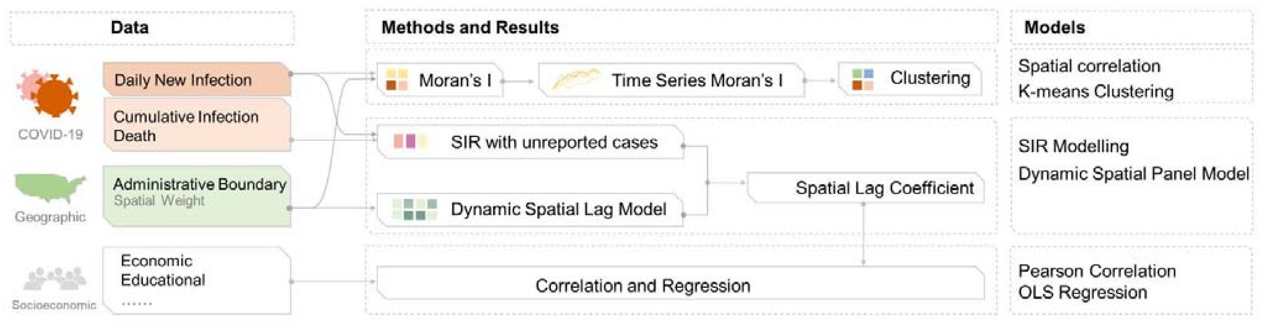
2. Materials and Methods

The workflow can be divided into three parts: (1) spatial autocorrelation analysis of daily new infections; (2) spatial effect exploration based on the SIRu model and Spatial Lag Model; and (3) correlation analysis of spatial effects and socio-economic factors (Figure 1).
The research workflow explains the data, methods, and models used in the article. Moran’s I and K-means clustering were introduced to capture the spatiotemporal features of COVID-19 daily new case changes in the U.S., then the spatial lag effect underlying the SIR model was further estimated via the SLM-SIRu model and further used for correlation tests with socio-economic variables.

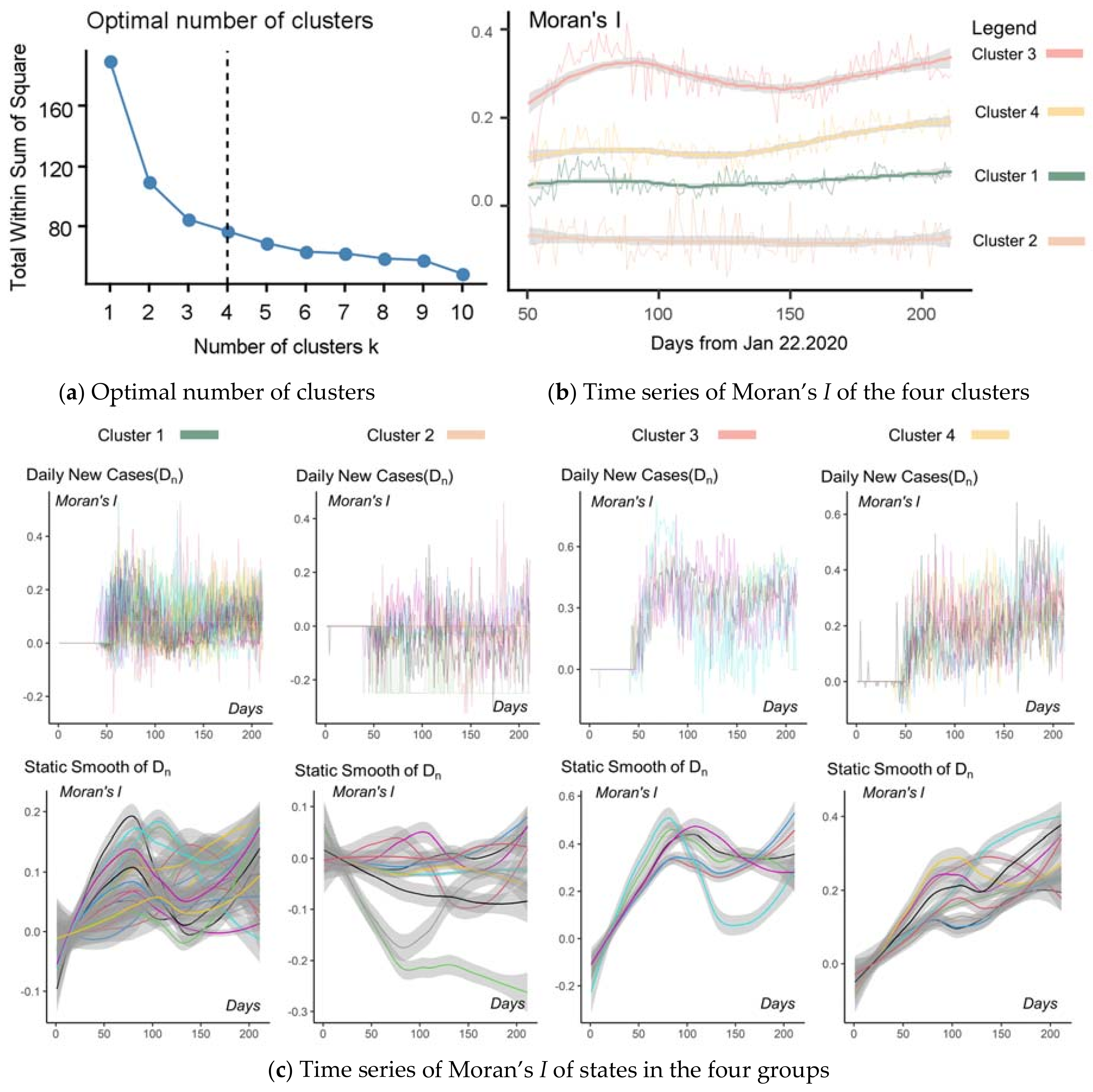
2.1. Global Moran’s I Index and K-Means Clustering

Except for extremely strict spatial restriction policies, any potential inter-county human movement between neighboring counties in a certain state may increase the contact chance and thus affect the number of daily new infections in each geographic unit. Such a pattern of spatial interaction in the state could be defined as spatial autocorrelation, which could be calculated using the global Moran’s I index based on spatial weights. The value of Moran’s I ranges from −1 to 1, where −1 represents a negative spatial correlation, 0 is random, and 1 is a positive correlation.
For a certain attribute x of geographic units, the general formula of global Moran’s I is
I = n W · i = 1 n j = 1 n w i , j x i x ¯ x j x ¯ i = 1 n x i x ¯ 2
wherein xi is the attribute value of the ith county in a state and x ¯ is the mean of all xi values in the state; xj represents the value of the jth county near to the ith county; n is the total number of counties; and W is the sum of spatial weights wij.
The spatial weight W can be calculated via a pre-defined neighboring pattern such as Queen, Rook, K-nearest, or inverse distances. The first two contiguity models rely on natural boundaries, while the latter only depends on a distance matrix.
Due to irregular administrative boundaries in some states, some counties may only have 1–2 neighborhood units, for which the popular Queen algorithm is applied. Thus, in order to ensure a relatively comparable neighborhood impact, the K-nearest model was selected, which calculates spatial weights with several nearest counties. The number k can be neither too small nor too large to characterize the local spatial interaction effect, so k was defined with a maximum value of 4—the same number for the Rook contiguity model. As there is only one unit in the District of Columbia, the spatial weight calculation could not be applied.
If the total number of infections or daily new infections of a state was zero, making the calculation of Equation (1) unapplicable, a value of zero was designated as the Moran’s I value of the corresponding state. Such a situation was also applied when the p-value of the Moran’s I calculation result was not significant (p > 0.05).

2.2. K-Means Clustering Algorithm

At different stages of COVID-19 transmission, the population movement among adjacent spatial units may change with the states’ control policies or the epidemic situation, resulting in Moran’s I index varying over time. The characteristics of the time series of Moran’s I index may reflect the spatial homogeneity and heterogeneity among the states in the United States, which could be explored by clustering algorithms.
The K-means clustering algorithm was applied as it can generate the guaranteed convergence and is relatively simple to implement compared to other clustering models such as DBSCAN or GMM. The optimal group number was determined by the minimum value of the AIC.

2.3. SIR with Unreported Infections

In the classic SIR model, the number of daily new infections (In) can be expressed as the product of the infected population (I), the susceptible population (S), the total population (N), and the transmission rate (β):
I n = β S I / N
However, the official data cannot be directly used, as there may be unreported infections. Moreover, the actual population of recovered patients has not been released in the county-level data, so the parameter I in Equation (2) could not be calculated directly. An SIR model integrated with unreported infections (SIRu) was proposed [37] by adding two more parameters, φ and τ, where φ is the average unreported/reported rate of infections (UIR) and τ is the recovery/death rate (RDR). Equation (2) could then be revised to
φ I n = β N φ I c φ I c τ R d / N
where In, Ic, and Rd are the official released COVID-19 data of daily new infections, cumulative infections, and deaths, respectively; therefore, φIn, φIc, and τRd are the corresponding factual data.
A furthermore simplification of Equation (3) can be rewritten as
I n = β I c β τ φ R d β φ I c 2 N + β τ I c R d N
Such an equation could be seen as a linear regression of the variables In, Ic, Rd, Ic2/N, and IcRd/N.

2.4. Dynamic Spatial Lag Model

Although the dynamic spatial panel models include the Spatial Lag Model (SLM), Spatial Error Model (SEM), and Spatial Dubin Model (SDM), the SLM was adapted to capture the spatial effect of the SIRu model, which focuses the impact of the new infections in surrounding counties on the increasing infection in a certain county. The SLM model only needs to add one variable, In, in Equation (3). If the SEM or SDM was applied, Equation (3) would become quite complicated by the addition of three other variables of neighboring units, which would also make Equation (4) inapplicable.
The classic SLM model could be described as
y = λ W y + a x + ε
wherein y is the dependent variable of a certain geographic unit, y′ represents the values of the adjacent geographic units, and x denotes the corresponding explanatory variables. W is the spatial weight, and λ is the spatial lag coefficient.
The SLM and SIRu models can be combined by substituting Equation (4) into Equation (5):
I n = λ W I n + β I c β τ φ R d β φ I c 2 N + β τ I c R d N
I n denotes the daily new infections of surrounding counties. Compared to Equation (4), only one variable, I n , is added in Equation (6). Based on the COVID-19 data at the county level and the corresponding spatial weights, the spatial interaction coefficient λ of each state can be calculated and used as a dependent variable for further correlation exploration with socioeconomic data.

2.5. Data

The data used in this article include COVID-19 data, geographic boundary data, and socioeconomic data, as follows:
(1)
COVID-19 data of all counties in the United States from 22 January 2020 to 20 August 2020, including daily new infections, cumulative infections, deaths, and total population. The data were acquired from the GitHub repository of Johns Hopkins University (https://github.com/CSSEGISandData/COVID-19, accessed on 21August 2020).
(2)
Administrative boundary data at the state and county levels in the United States. These data are available in the Harvard Dataverse (https://dataverse.harvard.edu/dataverse/cdl_dataverse, accessed on 21August 2020).
(3)
Socioeconomic data of all states in the United States in 2019, including factors such as birth rate, death rate, international immigration rate, poverty rate, median age, average education level (high school graduation rate, undergraduate graduation rate, advanced education rate), and population density. Such data are available on the U.S. Census website (https://www.census.gov, accessed on 30 August 2020). Trump’s vote rate in the 2016 U.S. presidential election in the states was also included in the correlation analysis as a potential political variable of residents.

3. Results

3.1. Time Series of Moran’s I

The time series of Moran’s I index for each state was calculated from the daily new cases and spatial weights at the county level for 22 January 2020 to 20 August 2020; these time series indicated that most states showed significant changes in terms of Moran’s I index (Figure 2). The spatial correlation within each state showed substantial differences over time; for example, New York maintained a restricted state after the first wave, while Georgia and Illinois were still increasing, and Florida had just passed the peak. Such time series of Moran’s I may reflect the real effects of spatial restriction policies.

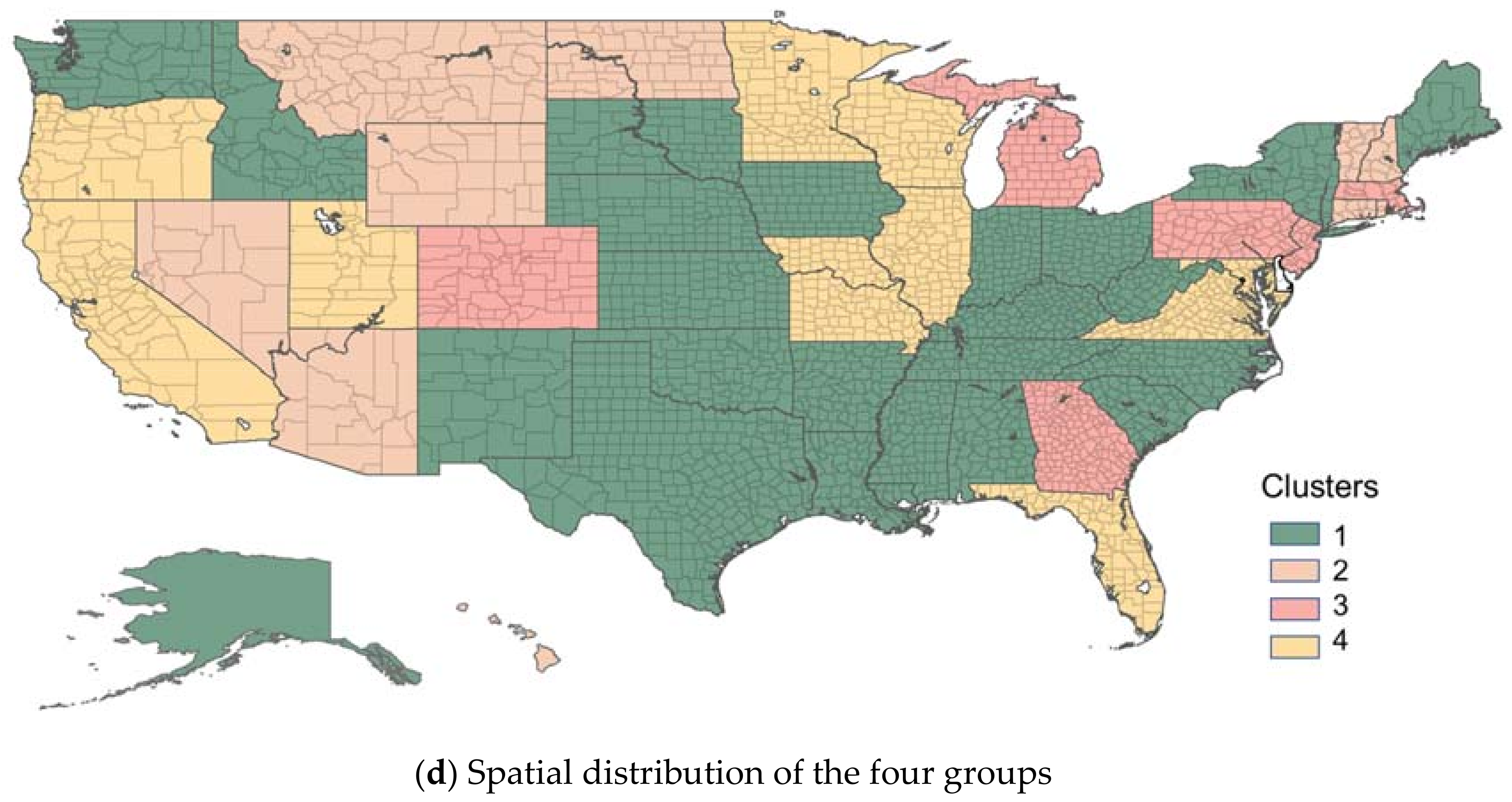
3.2. K-Means Clustering of Time Series of Moran’s I

The K-means clustering algorithm was further performed based on the time series of Moran’s I index. The results showed that the optimal group number was four (Figure 3a), and the four groups could be roughly defined as fluctuating growth, continuous growth, weak positive correlation, and weak negative correlation (Figure 3b). Figure 3c displays the Moran’s I values of each group, wherein the overall fluctuation range in Cluster 1 was −0.1 to 0.4, while the fitting curves and the 95% confidence interval were concentrated between −0.1 and 0.2, indicating a state of weakly positive spatial autocorrelation. Cluster 2, with a value ranging from −0.2 to 0.1, showed a feature of weakly negative spatial autocorrelation. Both Cluster 3 and Cluster 4 exhibited increasing trends, while the former was in a resurging status after the first wave and the latter was in a continuous increasing mode with a relatively lower value of Moran’s I. Figure 3d illustrates the clusters on the map, where the spatial agglomeration can also be observed.

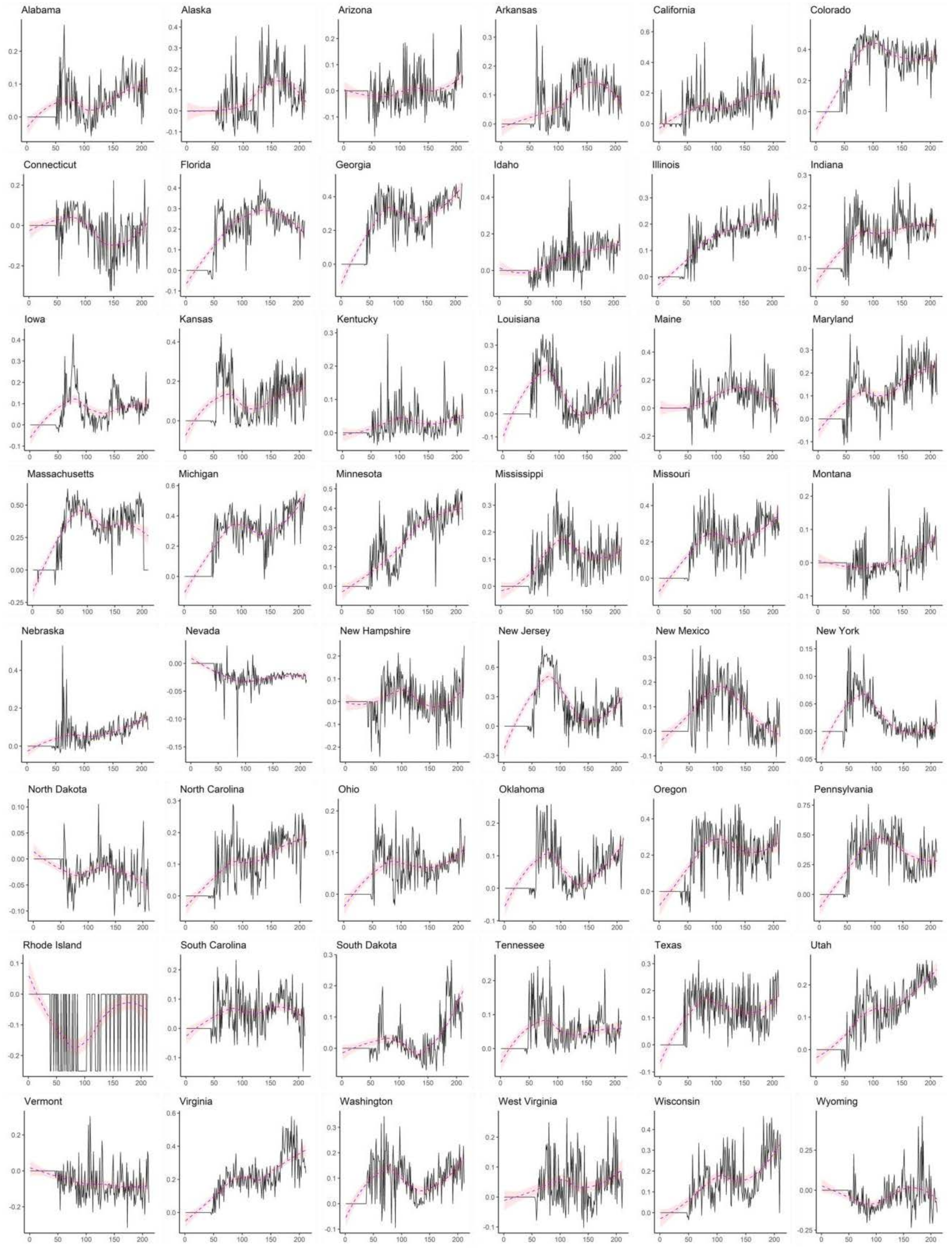
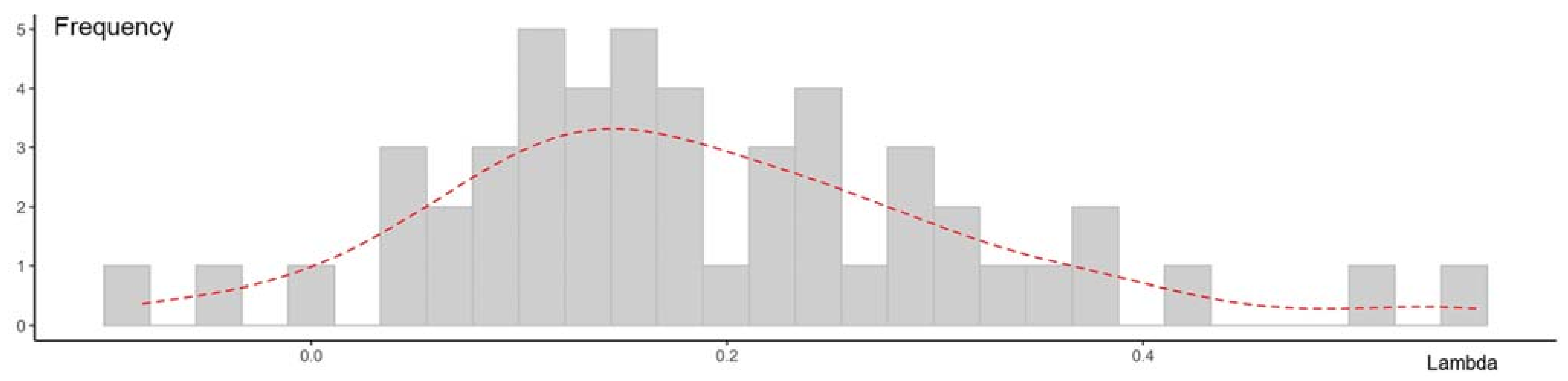
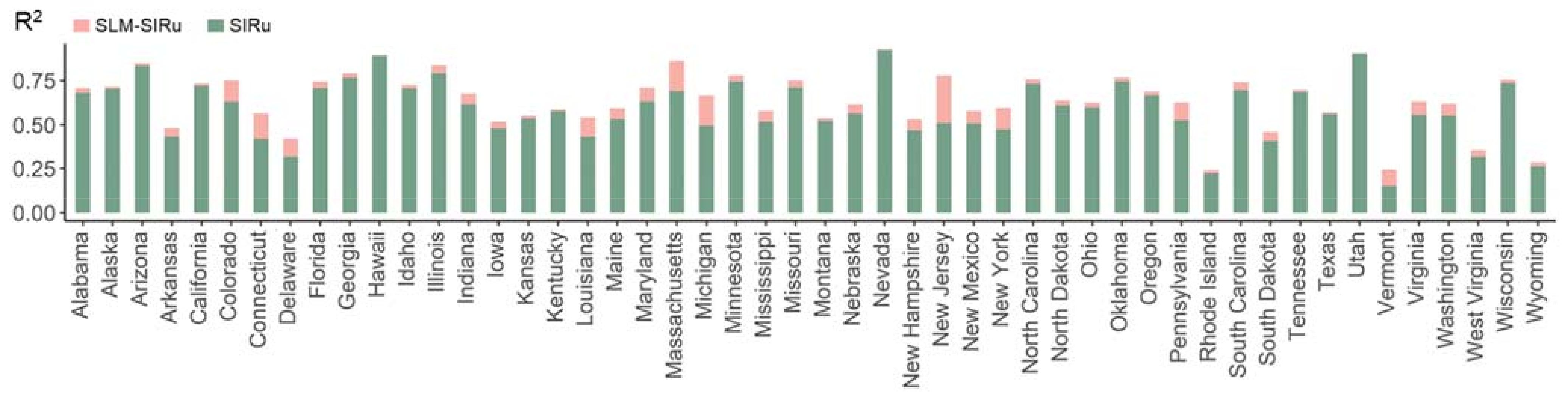
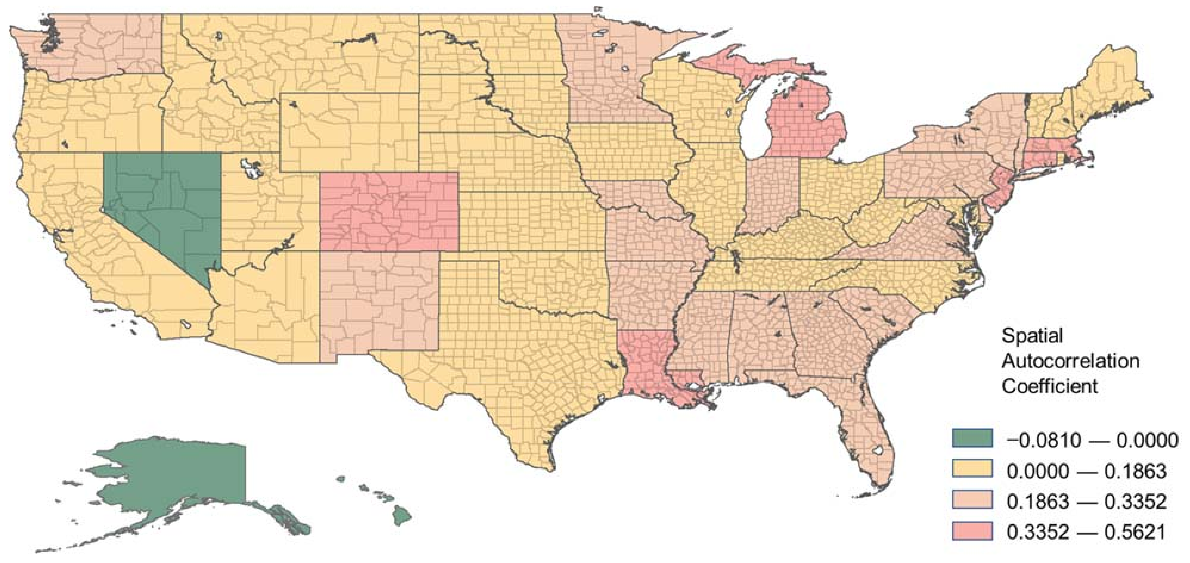
3.3. SIRu Integrated with the Spatial Lag Model

The combined SLM-SIRu model was tested with the spatial matrix and epidemic data of all the counties from 22 January 2020 to 20 August 2020. The results of all the states displayed high significance, verifying the feasibility of the SLM-SIRu model (Table 1). The parameter λ ranged from −0.08 to 0.56, showing a normal distribution (Figure 4). The SLM-SIRu model also showed high R2 values, most of which had a value larger than 0.5. In terms of fitness, the comparison between SIRu and SLM-SIRu indicated that the coefficient of spatial lag in SLM-SIRu improved the fitness of the original SIRu model (Figure 5).
Based on the mapping of the spatial autocorrelation coefficient λ with the four levels, it can be seen that only Alaska, Nevada, and Hawaii showed small negative values, while most of the central states had lower positive values, except for Colorado and New Mexico (Figure 6). The states in the southeast had similarly high values, among which Louisiana’s was the largest. In the north, Michigan, Massachusetts, Connecticut, and New Jersey also had relatively high spatial autocorrelation coefficients, indicating that the inter-county human flow in such states remains high.

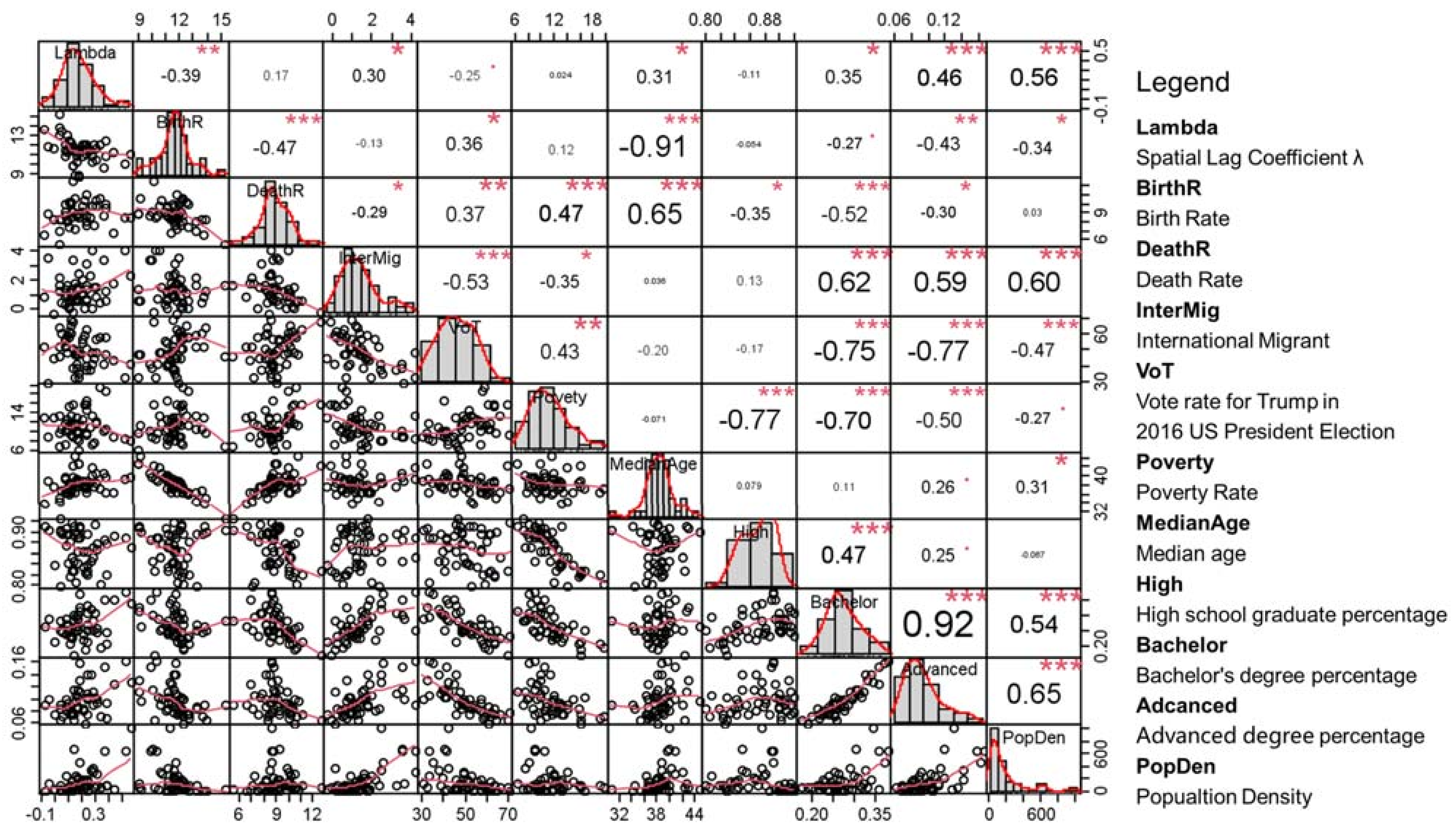
3.4. Correlation and Regression with Socioeconomic Variables

To explore the correlations between the social, economic, and political factors and spatial correlation coefficients, the Pearson correlation test was applied (Figure 7). The result showed a significant negative relationship with the birth rate and an obvious positive correlation with the proportion of international immigrants, median age, higher education rate, and population density. In terms of the political factor, President Trump’s support rate in the 2016 U.S. election showed a weak negative correlation (90% CI).
A further stepwise OLS review retained five variables, among which only three of the variables were significant: population density, poverty rate, and bachelor’s degree rate (Table 2). Among them, the population density and poverty rate were more significant, indicating that the intrastate population flow caused by population density and poverty was still dominant, and an increase in the highly educated population ratio would also increase the risk of inter-regional human flows.

4. Discussion

The initial objective of this project was to measure the inter-county spatiotemporal interaction effect of COVID-19 transmission in the United States and explore the correlations between the spatiotemporal interaction coefficients and socioeconomic features. The results of this study indicate that the inter-county spatial effects in these states are changing with time, displaying four types of spatial correlation trends: continuous increasing, fluctuating increasing, weak positive, and weak negative. The clustering of time series of the COVID-19 Moran’s I index, never previously reported, could be explained by the heterogeneity in the social and spatial peripheries [38].
The fitness of the SIRu models in all states had an average value above 0.75, indicating that the model can explain the epidemic dynamics of COVID-19 transmission in the United States. The SLM-SIRu model showed better fitness than the SIRu model with statistical significance, further verifying the hypothesis of spatial heterogeneity in epidemic dynamics [39]. The result indicates that the eastern states have a relatively high spatial interaction coefficient, showing a high possibility of inter-county flow.
In terms of socioeconomic features, the spatiotemporal interaction coefficients in each state were found to be positively correlated with the proportion of international immigrants, median age, proportion of highly educated population, and population density, but negatively correlated with the birth rate. The correlation in the two variables of median age and international immigrant ratio indicated that there is more cross-regional mobility to obtain living or medical equipment in those states with large ethnic minority populations and elderly populations, which verified that those residents in inequitable living, working, and environmental conditions may face a greater risk of COVID-19 infection [40]. What is interesting is that the vote rate for Donald Trump in the 2016 U.S. presidential election showed a weak negative correlation, which implies that political factors may also have some impact on the inter-county flow in the states [41].
The results of stepwise OLS regression suggested that the poverty rate, population density, and proportion of highly educated population are the three main positive correlated variables. Among these, the population density and poverty rate have been considered to be highly correlated to the COVID-19 transmission rate in previous studies [42,43], while our result implies that more inter-county flow may also occur in those states with higher population density or with low income in the United States. Such a result may support a study in Europe that proposed that high-population-density states appear to benefit more from their Shelter-in-Place Orders [44]. Of course, the cross-regional movement of highly educated people is also noteworthy, as these groups have better medical resources, better epidemic prevention knowledge, and lower infection rates [45], so the possible infection risk is relatively low and their mobility is thus less affected by policies of movement regularity. However, their unrestricted movement may bring risks to other vulnerable groups via direct or indirect disease contact. Low-income groups with worse protective equipment endure greater exposure risk when commuting between counties in search of reliable living and medical supplies [40]. The results of eliminating the political variable imply that although political factors are potentially related to the spread of epidemics, the dominant factors affecting infections between regions are still socioeconomic and demographic variables rather than political factors.
The spatiotemporal dynamic model established in this research still has many deficiencies in terms of spatial weight calculation and model optimization. On the one hand, for simplification, the spatial weights were calculated by the K-nearest algorithm based on counties in each state, while neglecting the inter-state spatial interaction, as COVID-19 transmission in each state not only occurs in adjacent counties but also emerges among different states. Future research can further calculate and compare spatial weight models such as the Queen neighbor algorithm and the inverse distance model based on travel network data, such as Twitter location data. On the other hand, the relevance was explored by spatial interaction effect measurement and OLS regression separately, which may be improved by a combined regression model. Moreover, the SLM model was chosen in this study due to the parameter limits; SDM and SEM may need further exploration. More models such as spatial dynamic SIR models or Neural network models could be tested in future. The SIRu model, adopted to adjust the impact of data depression, can also be further optimized in terms of accuracy.

5. Conclusions

This study proposes that inter-county movement within states has an impact on disease transmission, displaying obvious spatial heterogeneity that is potentially related to the social and economic factors of each state. This result suggests that governments should deploy targeted strategies in each state based on the estimation of spatiotemporal interaction effects; in particular, the states with greater estimated effects should strengthen regulations on human mobility. All states should provide more protection and support for the low-income population; high-population-density states need to strengthen regional mobility restrictions; and the highly educated group should reduce unnecessary regional movement and strengthen self-protection. In terms of vaccines and funds, it is suggested that the governments give priority to accelerating vaccination in cities with higher population density and increase the proportion of aid funds for low-income groups, rather than the current average implementation strategy.

Author Contributions

Lingbo Liu and Shuming Bao conceived and designed the experiments; Lingbo Li performed the experiments; Tao Hu and Zhenghong Peng acquired and analyzed the data; Ru Wang and Hao Wu contributed reagents/materials/analysis tools; Lingbo Liu wrote the paper. All authors have read and agreed to the published version of the manuscript.

Funding

The study was funded by the National Key Research and Development Project (2019YFB2101803); National Natural Science Foundation of China (52078390); and Wuhan University Experiment Technology Project Funding.

Institutional Review Board Statement

Not applicable.

Informed Consent Statement

Not applicable.

Data Availability Statement

The data used in this study were open-source data from Johns Hopkins University, available on GitHub (https://github.com/CSSEGISandData/COVID-19, accessed on 21 August 2020).

Acknowledgments

The authors would like to acknowledge the experts for their suggestions on the presentation of Data Statistical Analysis and Spatiotemporal Prediction Models of COVID-19 based on Workflow in the COVID-19 Data Analysis Webinar.

Conflicts of Interest

The authors declare no conflict of interest.

References

  1. Hu, T.; Guan, W.W.; Zhu, X.; Shao, Y.; Liu, L.; Du, J.; Liu, H.; Zhou, H.; Wang, J.; She, B.; et al. Building an open resources repository for COVID-19 research. Data Inf. Manag. 2020, 4, 130. [Google Scholar] [CrossRef]
  2. Yang, C.; Sha, D.; Liu, Q.; Li, Y.; Lan, H.; Guan, W.W.; Hu, T.; Li, Z.; Zhang, Z.; Thompson, J.H.; et al. Taking the pulse of COVID-19: A spatiotemporal perspective. Int. J. Digit. Earth 2020, 13, 1186–1211. [Google Scholar] [CrossRef]
  3. Loeffler-Wirth, H.; Schmidt, M.; Binder, H. Covid-19 transmission trajectories–monitoring the pandemic in the worldwide context. Viruses 2020, 12, 777. [Google Scholar] [CrossRef]
  4. Walker, P.G.T.; Whittaker, C.; Watson, O.J.; Baguelin, M.; Winskill, P.; Hamlet, A.; Djafaara, B.A.; Cucunubá, Z.; Olivera Mesa, D.; Green, W.; et al. The impact of COVID-19 and strategies for mitigation and suppression in low- and middle-income countries. Science 2020, 369, 413–422. [Google Scholar] [CrossRef] [PubMed]
  5. Dowd, J.B.; Andriano, L.; Brazel, D.M.; Rotondi, V.; Block, P.; Ding, X.; Liu, Y.; Mills, M.C. Demographic science aids in understanding the spread and fatality rates of COVID-19. Proc. Natl. Acad. Sci. USA 2020, 117, 9696. [Google Scholar] [CrossRef] [Green Version]
  6. Merlo, J.; Chaix, B.; Ohlsson, H.; Beckman, A.; Johnell, K.; Hjerpe, P.; Råstam, L.; Larsen, K. A brief conceptual tutorial of multilevel analysis in social epidemiology: Using measures of clustering in multilevel logistic regression to investigate contextual phenomena. J. Epidemiol. Commun. H 2006, 60, 290. [Google Scholar] [CrossRef] [Green Version]
  7. Qi, H.; Xiao, S.; Shi, R.; Ward, M.P.; Chen, Y.; Tu, W.; Su, Q.; Wang, W.; Wang, X.; Zhang, Z. COVID-19 transmission in Mainland China is associated with temperature and humidity: A time-series analysis. Sci. Total Environ. 2020, 728, 138778. [Google Scholar] [CrossRef]
  8. Wu, X.; Yin, J.; Li, C.; Xiang, H.; Lv, M.; Guo, Z. Natural and human environment interactively drive spread pattern of COVID-19: A city-level modeling study in China. Sci. Total Environ. 2021, 756, 143343. [Google Scholar] [CrossRef]
  9. Rader, B.; Scarpino, S.V.; Nande, A.; Hill, A.L.; Adlam, B.; Reiner, R.C.; Pigott, D.M.; Gutierrez, B.; Zarebski, A.E.; Shrestha, M.; et al. Crowding and the shape of COVID-19 epidemics. Nat. Med. 2020, 26, 1829–1834. [Google Scholar] [CrossRef]
  10. Roques, L.; Bonnefon, O.; Baudrot, V.; Soubeyrand, S.; Berestycki, H. A parsimonious approach for spatial transmission and heterogeneity in the COVID-19 propagation. R. Soc. Open Sci. 2020, 7, 201382. [Google Scholar] [CrossRef]
  11. Viguerie, A.; Lorenzo, G.; Auricchio, F.; Baroli, D.; Hughes, T.J.R.; Patton, A.; Reali, A.; Yankeelov, T.E.; Veneziani, A. Simulating the spread of COVID-19 via a spatially-resolved susceptible–exposed–infected–recovered–deceased (SEIRD) model with heterogeneous diffusion. Appl. Math. Lett. 2021, 111, 106617. [Google Scholar] [CrossRef]
  12. Adekunle, I.A.; Onanuga, A.T.; Akinola, O.O.; Ogunbanjo, O.W. Modelling spatial variations of coronavirus disease (COVID-19) in Africa. Sci. Total Environ. 2020, 729, 138998. [Google Scholar] [CrossRef]
  13. Xiong, C.; Hu, S.; Yang, M.; Luo, W.; Zhang, L. Mobile device data reveal the dynamics in a positive relationship between human mobility and COVID-19 infections. Proc. Natl. Acad. Sci. USA 2020, 117, 27087. [Google Scholar] [CrossRef]
  14. Aleta, A.; Martín-Corral, D.; Pastore y Piontti, A.; Ajelli, M.; Litvinova, M.; Chinazzi, M.; Dean, N.E.; Halloran, M.E.; Longini, I.M., Jr.; Merler, S.; et al. Modelling the impact of testing, contact tracing and household quarantine on second waves of COVID-19. Nat. Hum. Behav. 2020, 4, 964–971. [Google Scholar] [CrossRef]
  15. Ascani, A.; Faggian, A.; Montresor, S. The geography of COVID-19 and the structure of local economies: The case of Italy. J. Reg. Sci. 2020. [Google Scholar] [CrossRef]
  16. Hellewell, J.; Abbott, S.; Gimma, A.; Bosse, N.I.; Jarvis, C.I.; Russell, T.W.; Munday, J.D.; Kucharski, A.J.; Edmunds, W.J.; Sun, F. Feasibility of controlling COVID-19 outbreaks by isolation of cases and contacts. Lancet Glob. Health 2020, 8, e488–e496. [Google Scholar] [CrossRef] [Green Version]
  17. Abel, T.; Mcqueen, D. The COVID-19 pandemic calls for spatial distancing and social closeness: Not for social distancing! Int. J. Public Health 2020, 65, 231. [Google Scholar] [CrossRef] [Green Version]
  18. Lai, S.; Ruktanonchai, N.W.; Zhou, L.; Prosper, O.; Luo, W.; Floyd, J.R.; Wesolowski, A.; Santillana, M.; Zhang, C.; Du, X.; et al. Effect of non-pharmaceutical interventions to contain COVID-19 in China. Nature 2020, 585, 410–413. [Google Scholar] [CrossRef]
  19. Kraemer, M.U.G.; Yang, C.-H.; Gutierrez, B.; Wu, C.-H.; Klein, B.; Pigott, D.M.; du Plessis, L.; Faria, N.R.; Li, R.; Hanage, W.P.; et al. The effect of human mobility and control measures on the COVID-19 epidemic in China. Science 2020, 368, 493. [Google Scholar] [CrossRef] [Green Version]
  20. Flaxman, S.; Mishra, S.; Gandy, A.; Unwin, H.J.T.; Mellan, T.A.; Coupland, H.; Whittaker, C.; Zhu, H.; Berah, T.; Eaton, J.W.; et al. Estimating the effects of non-pharmaceutical interventions on COVID-19 in Europe. Nature 2020, 584, 257–261. [Google Scholar] [CrossRef]
  21. Bertuzzo, E.; Mari, L.; Pasetto, D.; Miccoli, S.; Casagrandi, R.; Gatto, M.; Rinaldo, A. The geography of COVID-19 spread in Italy and implications for the relaxation of confinement measures. Nat. Commun. 2020, 11, 4264. [Google Scholar] [CrossRef] [PubMed]
  22. Liu, F.; Wang, J.; Liu, J.; Li, Y.; Liu, D.; Tong, J.; Li, Z.; Yu, D.; Fan, Y.; Bi, X.; et al. Predicting and analyzing the COVID-19 epidemic in China: Based on SEIRD, LSTM and GWR models. PLoS ONE 2020, 15, e0238280. [Google Scholar] [CrossRef]
  23. Das, A.; Ghosh, S.; Das, K.; Basu, T.; Dutta, I.; Das, M. Living environment matters: Unravelling the spatial clustering of COVID-19 hotspots in Kolkata megacity, India. Sustain. Cities Soc. 2020, 102577. [Google Scholar] [CrossRef]
  24. Fingleton, B.; Olner, D.; Pryce, G. Estimating the local employment impacts of immigration: A dynamic spatial panel model. Urban. Stud. 2019, 57, 2646–2662. [Google Scholar] [CrossRef] [Green Version]
  25. Sannigrahi, S.; Pilla, F.; Basu, B.; Basu, A.S.; Molter, A. Examining the association between socio-demographic composition and COVID-19 fatalities in the European region using spatial regression approach. Sustain. Cities Soc. 2020, 62, 102418. Available online: https://0-www-sciencedirect-com.brum.beds.ac.uk/science/article/pii/S2210670720306399 (accessed on 21 December 2020). [CrossRef]
  26. Mollalo, A.; Vahedi, B.; Rivera, K.M. GIS-based spatial modeling of COVID-19 incidence rate in the continental United States. Sci. Total Environ. 2020, 728, 138884. [Google Scholar] [CrossRef]
  27. Anderson, R.M.; Heesterbeek, H.; Klinkenberg, D.; Hollingsworth, T.D. How will country-based mitigation measures influence the course of the COVID-19 epidemic? Lancet 2020, 395, 931–934. [Google Scholar] [CrossRef]
  28. Lau, H.; Khosrawipour, V.; Kocbach, P.; Mikolajczyk, A.; Ichii, H.; Schubert, J.; Bania, J.; Khosrawipour, T. Internationally lost COVID-19 cases. J. Microbiol. Immunol. Infect. 2020, 53, 454–458. [Google Scholar] [CrossRef]
  29. Spychalski, P.; Błażyńska-Spychalska, A.; Kobiela, J. Estimating case fatality rates of COVID-19. Lancet Infect. Dis. 2020, 20, 774–775. [Google Scholar] [CrossRef]
  30. Wu, S.L.; Mertens, A.N.; Crider, Y.S.; Nguyen, A.; Pokpongkiat, N.N.; Djajadi, S.; Seth, A.; Hsiang, M.S.; Colford, J.M.; Reingold, A.; et al. Substantial underestimation of SARS-CoV-2 infection in the United States. Nat. Commun. 2020, 11, 4507. [Google Scholar] [CrossRef]
  31. Leon, D.A.; Shkolnikov, V.M.; Smeeth, L.; Magnus, P.; Pechholdová, M.; Jarvis, C.I. COVID-19: A need for real-time monitoring of weekly excess deaths. Lancet 2020, 395, e81. [Google Scholar] [CrossRef]
  32. Lipsitch, M.; Donnelly, C.A.; Fraser, C.; Blake, I.M.; Cori, A.; Dorigatti, I.; Ferguson, N.M.; Garske, T.; Mills, H.L.; Riley, S.; et al. Potential biases in estimating absolute and relative case-fatality risks during outbreaks. PLoS Neglect. Trop D 2015, 9, e0003846. [Google Scholar] [CrossRef] [PubMed] [Green Version]
  33. Verity, R.; Okell, L.C.; Dorigatti, I.; Winskill, P.; Whittaker, C.; Imai, N.; Cuomo-Dannenburg, G.; Thompson, H.; Walker, P.G.T.; Fu, H.; et al. Estimates of the severity of coronavirus disease 2019: A model-based analysis. Lancet Infect. Dis. 2020, 20, 669–677. [Google Scholar] [CrossRef]
  34. Liu, Z.; Magal, P.; Seydi, O.; Webb, G. A COVID-19 epidemic model with latency period. Infect. Dis. Model. 2020, 5, 323–337. [Google Scholar] [CrossRef] [PubMed]
  35. Cave, B.; Kim, J.; Viliani, F.; Harris, P. Applying an equity lens to urban policy measures for COVID-19 in four cities. Cities Health 2020, 1–5. [Google Scholar] [CrossRef]
  36. Hamidi, S.; Sabouri, S.; Ewing, R. Does density aggravate the COVID-19 pandemic? Early findings and lessons for planners. J. Am. Plan. Assoc. 2020, 1–15. [Google Scholar] [CrossRef]
  37. Peng, Z.; Ao, S.; Liu, L.; Bao, S.; Hu, T.; Wu, H.; Wang, R. Estimating unreported COVID-19 cases with a time-varying SIR regression model. Int. J. Environ. Res. Public Health 2021, 18, 1090. [Google Scholar] [CrossRef]
  38. Biglieri, S.; De Vidovich, L.; Keil, R. City as the core of contagion? Repositioning COVID-19 at the social and spatial periphery of urban society. Cities Health 2020, 1–3. [Google Scholar] [CrossRef]
  39. Sun, F.; Matthews, S.A.; Yang, T.-C.; Hu, M.-H. A spatial analysis of the COVID-19 period prevalence in U.S. counties through 28 June 2020: Where geography matters? Ann. Epidemiol. 2020, 52, 54–59. [Google Scholar] [CrossRef]
  40. Cole, H.V.S.; Anguelovski, I.; Baró, F.; García-Lamarca, M.; Kotsila, P.; Pérez del Pulgar, C.; Shokry, G.; Triguero-Mas, M. The COVID-19 pandemic: Power and privilege, gentrification, and urban environmental justice in the global north. Cities Health 2020, 1–5. [Google Scholar] [CrossRef]
  41. Yamey, G.; Gonsalves, G. Donald Trump: A political determinant of COVID-19. BMJ 2020, 369, m1643. [Google Scholar] [CrossRef] [Green Version]
  42. White, E.R.; Hébert-Dufresne, L. State-level variation of initial COVID-19 dynamics in the United States. PLoS ONE 2020, 15, e0240648. [Google Scholar] [CrossRef]
  43. Berkowitz, R.L.; Gao, X.; Michaels, E.K.; Mujahid, M.S. Structurally vulnerable neighbourhood environments and racial/ethnic COVID-19 inequities. Cities Health 2020, 1–4. [Google Scholar] [CrossRef]
  44. Dave, D.; Friedson, A.I.; Matsuzawa, K.; Sabia, J.J. When do shelter-in-place orders fight COVID-19 best? Policy heterogeneity across states and adoption time. Econ. Inq. 2021, 59, 29–52. [Google Scholar] [CrossRef]
  45. Cordes, J.; Castro, M.C. Spatial analysis of COVID-19 clusters and contextual factors in New York City. Spat. Spatio Temporal Epidemiol. 2020, 34, 100355. [Google Scholar] [CrossRef]
Figure 1. Research workflow. The research workflow can be divided into three parts: (1) data, including epidemiological, spatial, and socioeconomic data; (2) methods and results, including the mapping, estimation, and correlation exploration of spatiotemporal interaction effects; and (3) models, including Moran’s I, K-means clustering, SIR, SLM, and OLS.
Ijgi 10 00387 g001
Figure 2. Time series of the Moran’s I index of each state in the United States. The x-axis and y-axis indicate the time in days and Moran’s I value, correspondingly, and the red curve represents the fitted value with a 95% confidence interval. Obvious changes from around the 50th day can be observed, displaying several patterns of temporal changes in spatial effects, such as a reversed U-shape or N-shape. There were zero values in the numbers of daily new infections for Rhode Island, which caused the Moran’s I curve to swing back and forth from 0 to negative values.
Ijgi 10 00387 g002
Figure 3. Time series of Moran’s I index for each state in the United States. The time series of the Moran’s I value from the 50th day were used for K-means clustering, as the values of most states were zero before the 50th day. (a) The AIC of the clustering algorithm achieved the minimum value when the number of clusters was four. (b) The four curves with grey ribbons represent the corresponding values and 95% CIs of the fitted lines of the four clusters. (c) The upper images show the original curves of the Moran’s I value, and the lower ones show the fitted trends and 95% CIs. (d) Most of the states belonged to Cluster 1, while Cluster 2 was mainly located in the middle. Although the states in Cluster 3 were dispersed, Cluster 4 displayed a pattern of spatial aggregation.
Ijgi 10 00387 g003aIjgi 10 00387 g003b
Figure 4. Histogram and density plot of spatial correlation coefficient λ. The grey bars in Figure 4 show the frequency of λ values, and the red line is the Probability Density Function (PDF) curve of the λ values.
Ijgi 10 00387 g004
Figure 5. Fitness comparison of SLM-SIRu and SIRu. The R2 range of the original SIRu was 0.1490–0.9250 (mean = 0.5894), while that of SLM-SIRu was 0.2399–0.9303 (mean = 0.6443); thus, the percentage of R2 improvement was 0.35%–62.72% with a mean of 11.54%.
Ijgi 10 00387 g005
Figure 6. The choropleth map of spatial correlation coefficient λ. For the choropleth map of the spatial correlation coefficient λ, shown in Figure 6, we used the Jerkens breakpoints with four levels.
Ijgi 10 00387 g006
Figure 7. The correlation tests between λ and socioeconomic variables. The left part under the diagonal line in Figure 7 shows the scatter point plots, and the numbers are the correlation coefficients. The diagrams along the diagonal line are the histograms. Notes: ***, **, *, and · mean that correlation is significant at the 0.001, 0.01, 0.05, and 0.1 levels, correspondingly.
Ijgi 10 00387 g007
Table 1. Summary of spatial lag coefficients in the SLM-SIRu model.
StateSpatial Lag CoefficientStand Errort-Valuep-Value
Alabama0.2297 ***0.008427.2015<0.001
Alaska−0.081 ***0.0126−6.4374<0.001
Arizona0.09 ***0.01247.2636<0.001
Arkansas0.2168 ***0.009921.8995<0.001
California0.1472 ***0.009814.9829<0.001
Colorado0.4275 ***0.008351.6714<0.001
Connecticut0.3625 ***0.023315.5821<0.001
Delaware0.278 ***0.03108.9794<0.001
Florida0.2826 ***0.008134.6982<0.001
Georgia0.2395 ***0.005147.2483<0.001
Hawaii−0.0489 **0.0197−2.48830.0128
Idaho0.1117 ***0.008812.7027<0.001
Illinois0.1661 ***0.006625.0248<0.001
Indiana0.2052 ***0.008424.3700<0.001
Iowa0.1312 ***0.008715.0073<0.001
Kansas0.0773 ***0.00819.5291<0.001
Kentucky0.1032 ***0.007813.237<0.001
Louisiana0.3791 ***0.008644.0066<0.001
Maine0.1497 ***0.02147.004<0.001
Maryland0.1864 ***0.014912.5354<0.001
Massachusetts0.5202 ***0.011146.704<0.001
Michigan0.3771 ***0.007550.2282<0.001
Minnesota0.2892 ***0.007339.4947<0.001
Mississippi0.3353 ***0.008141.2161<0.001
Missouri0.3031 ***0.006546.2933<0.001
Montana0.0859 ***0.01078.0393<0.001
Nebraska0.1004 ***0.008511.7588<0.001
Nevada−0.0036 **0.0168−0.2142 *0.0184
New Hampshire0.1856 ***0.02657.0142<0.001
New Jersey0.5621 ***0.011449.3291<0.001
New Mexico0.2381 ***0.012818.5421<0.001
New York0.2663 ***0.009029.7591<0.001
North Carolina0.1598 ***0.007122.449<0.001
North Dakota0.0348 **0.01123.1114 **0.0019
Ohio0.0812 ***0.00909.0392<0.001
Oklahoma0.1172 ***0.007515.6807<0.001
Oregon0.1709 ***0.012613.5983<0.001
Pennsylvania0.3031 ***0.008834.2476<0.001
Rhode Island0.1400 ***0.03713.7685<0.001
South Carolina0.2134 ***0.009522.4236<0.001
South Dakota0.0560 ***0.01174.8008<0.001
Tennessee0.1216 ***0.007915.3701<0.001
Texas0.0376 ***0.00527.2084<0.001
Utah0.0377 ***0.00894.2494<0.001
Vermont0.1746 ***0.02437.1958<0.001
Virginia0.2374 ***0.006337.9368<0.001
Washington0.2351 ***0.012618.6703<0.001
West Virginia0.1351 ***0.011911.3082<0.001
Wisconsin0.1627 ***0.007820.7673<0.001
Wyoming0.1288 ***0.01886.8477<0.001
Notes: ***, ** and * means correlation significant at the level of 0.001, 0.01 and 0.05, respectively.
Table 2. Summary of stepwise OLS regression.
EstimateStd. Errort-Valuep-ValueVIF
Intercept0.00000.10930.0001.0000
BirthR−0.24190.1214−1.9920.05251.208749
VoT0.26690.17521.5230.13492.518246
Poverty0.4468 **0.15892.8100.00732.072469
Bachelor0.5706 *0.22922.4890.01664.310079
PopDen0.4089 **0.13712.9830.00461.541248
Multiple R20.4633
Adjusted R20.4023
p-value0.00003247
Notes: **, and * mean that correlation is significant at the 0.01, and 0.05 levels, correspondingly.
Publisher’s Note: MDPI stays neutral with regard to jurisdictional claims in published maps and institutional affiliations.

