
INS Error Estimation Based on an ANFIS and Its Application in Complex and Covert Surroundings

School of Environment Science and Spatial Informatics, China University of Mining and Technology, Xuzhou 221116, China
*
Author to whom correspondence should be addressed.
ISPRS Int. J. Geo-Inf. 2021, 10(6), 388; https://0-doi-org.brum.beds.ac.uk/10.3390/ijgi10060388
Submission received: 26 April 2021
/
Revised: 31 May 2021
/
Accepted: 3 June 2021
/
Published: 4 June 2021
(This article belongs to the Special Issue Advances in Localization and Navigation (GIS Ostrava 2021))
Abstract
:Inertial navigation is a crucial part of vehicle navigation systems in complex and covert surroundings. To address the low accuracy of vehicle inertial navigation in multifaced and covert surroundings, in this study, we proposed an inertial navigation error estimation based on an adaptive neuro fuzzy inference system (ANFIS) which can quickly and accurately output the position error of a vehicle end-to-end. The new system was tested using both single-sequence and multi-sequence data collected from a vehicle by the KITTI dataset. The results were compared with an inertial navigation system (INS) position solution method, artificial neural networks (ANNs) method, and a long short-term memory (LSTM) method. Test results indicated that the accumulative position errors in single sequence and multi-sequences experiments decreased from 9.83% and 4.14% to 0.45% and 0.61% by using ANFIS, respectively, which were significantly less than those of the other three approaches. This result suggests that the ANFIS can considerably improve the positioning accuracy of inertial navigation, which has significance for vehicle inertial navigation in complex and covert surroundings.
Keywords:
INS solution; vehicle navigation; ANFIS; error estimation; ANNs; accumulative position error; LSTM1. Introduction
With the increasing requirements of vehicle navigation accuracy, improving vehicle navigation performance is a popular research topic. The commonly used sensors in navigation include GPS (global positioning system), INS (inertial navigation system), camera, odometer, lidar, etc. [1]. However, in complex and covert surroundings such as indoors, underground, in forests, and even in celestial bodies, GPSs can hardly provide continuous and accurate positioning. As a low-cost relative positioning sensor not affected by topography and surroundings, INS has played an important role in calculating vehicle poses [2]. An inertial measurement unit (IMU) is the hardware of an INS. Compared with GPS measurement technology, an IMU is hardly impacted by complex surroundings and has the advantage of high sampling rates. However, the position calculated by the accelerometers and gyroscopes accumulate errors over time. The common solution is to use GPS and INS integration for loosely coupled and tightly coupled [3]. Moreover, cameras, odometers, lidars, and other light- and sound-sensitive sensors are often used for integrated navigation and positioning, with INSs used for indoors, underground, the moon, planets, and other complex surroundings where GPS is not applicable [4,5,6]; this is expensive and computationally complicated. When the GPS signal is blocked for a long time without the aid of other sensors, the error of the position obtained by an INS is most likely to be large, which is the major problem to be solved in this study. In this case, a machine learning method can be used to compensate for the error. Currently, the commonly used solutions are the utilizing of artificial neural networks [7], delayed neural networks [8], adaptive neural fuzzy inference system (ANFIS) [9,10], and other neural networks [11] to estimate the errors of the integrated system consisting of GPSs, IMUs, odometers, and other sensors which can output more accurate positioning results in real-time or quasi-real-time. However, these methods require additional sensors, which generally increase training time. There are also some studies in the literature about IMU de-noising by using machine learning methods [12,13,14]. Some studies estimate the position and velocity errors end-to-end by only using an IMU when GPS outages occur; this is attempted mainly using artificial neural networks (ANNs) [15], recurrent neural networks (RNNs) [16], long short-term memory (LSTM) [17], convolutional neural networks (CNNs) [18], support vector machines (SVM) [19], and other machine learning algorithms [20,21,22]. As the high data collection frequency of the INS, these methods lead to the long training time of the model. Generally, machine learning is employed to estimate and correct the accumulative error in the position or velocity of the IMU; however, the main issues of the method are its low accuracy and long training time.
An accumulative error in the position of the IMU estimation model based on an adaptive neuro fuzzy inference system is proposed in this study to address the above problems. Using only INS observations, this model could effectively reduce the algorithmic complexity and shorten the training time compared with other machine learning methods. It can obtain the position of vehicles in complex and covert surroundings where GPS signals are missing or are not available for an extended period. In addition, a Karlsruhe Institute of Technology and Toyota Technological Institute (KITTI) unrectified raw dataset was used to validate the results of the new algorithm, and the differential GPS data of the dataset were used as the reference position to learn the position error of the INS solution and predict the subsequent position error. Experimental results indicated that the proposed model can estimate and correct the position error of the INS solution with high accuracy. The improvements made in this study can be summarized in three points: (i) Compared with other articles in the literature [9,10,23,24,25,26,27,28,29], time stamps were used as the inputs, which can shuffle date in this time-series problem and enhance the robustness of the training model. (ii) This study uses ANFIS to estimate the IMU error over an extended period. In contrast, GPS/IMU integration is widely used to estimate the carrier trajectory by using ANFIS within a short time of GPS outage [10,23,24,25,26,27,28]. (iii) Considering that the error will increase after two-dimensional integration, the position error was directly estimated without de-noising [14]. The findings of this study have theoretical and practical significance for improving the positioning accuracy of vehicles’ inertial navigation in complex and covert surroundings and provide technical support for vehicle navigation in complex surroundings.
2. Methods
In this section, the algorithm of the INS solution and ANFIS is presented. The principles, basic equations, and information flow are briefly introduced.
2.1. INS Solution
An INS can be either a gimbaled inertial navigation system (GINS) or a strapdown inertial navigation system (SINS), depending on the availability of a physical platform. SINSs were the main focus of this study for calculating the position of the vehicles [30]. An IMU is a component of an inertial navigation system, generally composed of a three-axis gyroscope and a three-axis accelerometer. Under a given initial condition, only the observations of an IMU can be calculated to estimate the position, velocity, and acceleration of the vehicle in the body coordinate system (b system) of the vehicle or a geographic coordinate system (n system).
2.1.1. Inertial Navigation Observation Model
As an IMU is directly installed on the vehicle of a SINS, its accelerometer and gyroscope can record the motion information of the vehicle, and the coordinate system of the measurements is in the b system. Let the observations of the IMU at a particular moment be
where L is the vector of the 6-D observations from the accelerometer and gyroscope; is the true value of L; and is the error of L, which can be expressed as
where is the IMU error, which mainly contains the zero offset of the accelerometer, the zero drift of the gyroscope, the temperature drift of the two sensors, and the reading error caused by the special motion state; is the initialization error, including the initial alignment and calibration error of the IMU; is the calculation error, including the initial condition error and higher-order term error of the integration; and includes all other errors.
2.1.2. Position Calculation by Using INS Observations
INS is not a Lyapunov stable system due to the non-linear and dynamic estimation system used for the INS solution. As a result, any minuscule external interference may change the error propagation. In this study, instead of performing error compensation under the initial conditions, the above errors were modeled as a whole, and the observations of the IMU were directly used to estimate the vehicle’s pose. Let
where Acc is the observations of the 3-D accelerometers, including the acceleration of the vehicle and the gravitational acceleration G in the n system; Gyr is the observations of the 3-D gyroscopes in the b system. Then, the acceleration of the vehicle in the n system can be obtained from the following transformation
where
is the orthogonal matrix denoting the transformation from the n system to the b system; φ, θ, and ψ are the angles of roll, pitch, and yaw angles, respectively, which are also the observations of the IMU gyroscopes, i.e., Gyr = [φ θ ψ]T
By integrating the acceleration of the vehicle in Equation (4), the velocity of the vehicle at the moment t in the n system can be obtained by
where is the velocity of the vehicle at the initial time. Then, the position of the vehicle at time t can be derived as
where is the position of the vehicle in the n system at the initial time.
Since the b system moves with the vehicle, to express the motion state of the vehicle relative to the surroundings, the pose of the vehicle at the initial time in the b system is called the b0 system and, similarly to Equations (4)–(7), the position of the vehicle at time t in the b0 system can be obtained by
where is the vehicle’s position in the b0 system at time t; is the rotation matrix from the n system to the b0 system at the initial time.
To describe the position and posture of the vehicle, a homogeneous matrix is used:
where is defined as the transformation matrix at time t, which is a special Euclidean group. Let
be the pose matrix, and . The first term of the matrix is the vehicle’s attitude at time t relative to the initial time, and the second term is the vehicle’s position at time t relative to the initial time.
2.2. ANFIS and Its Structure
The ANFIS is an ANN-based on a fuzzy inference system (FIS). It is, in fact, the integration of neural networks and fuzzy logic; hence it has the advantages of both and is introduced below.
2.2.1. Fuzzy Inference System
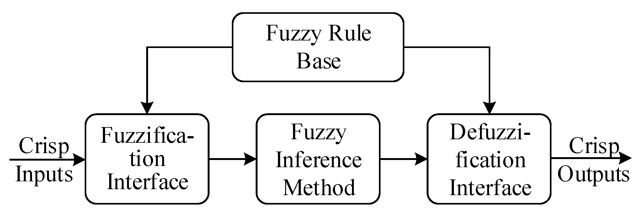
A fuzzy inference system is a system with crisp inputs and outputs, and the theory of fuzzy logic is its primary calculation tool. It imitates comprehensive human inference to cope with fuzzy information that is arduous to be solved by conventional mathematical methods and is mainly applied to resolve non-linear mapping issues [31]. It has been widely applied in unravel sequential signal processing, pattern recognition, automatic control, image processing, and other fields [32,33]. A fuzzy inference system is mainly composed of a fuzzification interface, a fuzzy rule base, a fuzzy inference method, and a defuzzification interface. The relationship between these modules is shown in Figure 1.
The fuzzification interface is used to apply a membership function (MF) for converting the crisp inputs into a fuzzy set. The fuzzy set at the crisp value should have a high membership degree, and the fuzzification result should have the capability to perform anti-jamming. Commonly used membership functions are the triangular function, the trapezoidal function, the Gaussian membership function, and the generalized bell-shaped membership function [34]. In this study, the Gaussian membership function was adopted, and its membership function value of the j-th input value of the i-th rule is defined as
where x is the crisp input; c represents the center of the membership function curve; σ is the width of the membership function. The defuzzification interface is to determine a crisp value that can best represent the fuzzy set. The fuzzy rule base is ordinarily defined as the fuzzy if-then rules, which simulate the inference mechanism of humans making judgments in uncertain and inaccurate surroundings. The other modules of the FIS serve the fuzzy rule base to make more effective judgments. The i-th rule denoted by Ri is usually expressed as
where . is the vector of the input values; y is the output value; A is the fuzzy set obtained by Equation (11); B is the polynomial related to x. The fuzzy inference method performs reasoning operations on fuzzy rules, and common approaches include the Mamdani inference method, the Larsen inference method, the Zadeh inference method, the T-S (Takagi–Sugeno) inference method, etc. [35]. Assuming that the number of rules set by the inference system is m, the fuzzy factor can be defined as
The output can be obtained from the weighted mean formula as follows
2.2.2. Artificial Neural Networks
ANN [36] is a mathematical model that imitates the structure and function of biological neural networks to solve non-linear problems [37]. ANN aims to obtain the activation function value of each neuron and the weights between the neurons of adjacent network layers when the cost function value is minimized.
The cost function of the back propagation algorithm (BP algorithm) is
where n is the total number of training samples; K is the output dimension, the second term of J(Θ) is the L2 regular term; λ is the regularization coefficient; L is the number of the network layers; sl is the number of the neurons in the l layer; hΘ (xi) gives the output of the neural network; y denotes the target value of the samples; represents the connection weight between the j-th neuron in the l-th layer and the m-th neuron in the (l + 1)-th layer. The phenomenon of over-fitting can be circumvented by introducing the regularization term into the cost function, while matrix irreversibility can be avoided with the regularization term (when λ > 0) when solving the minimum cost function. Commonly used methods include the gradient descent method, the quasi-Newton method, the conjugate gradient method [38], and heuristic methods such as genetic and simulated annealing algorithms [39] to calculate the cost function. This study used the quasi-Newton BFGS algorithm to calculate the minimum cost function [40]. Compared with the traditional gradient descent method, its convergence is faster at the minimum value, and it is easier to achieve the global optimal value. Compared to the Newton method, it simplifies the complexity of the operation because it does not need to calculate the Hessian matrix.
The number of hidden layers and the number of neurons in the hidden layer are the main parameters that affect the accuracy and complexity of the model. It is generally argued that an appropriate increase in the number of hidden layers for the time sequence issues can decrease the model error, but an excessively high hidden layer will increase this error. In the BP algorithm, the gradient value decreases as the number of the hidden layers increases and gradually approaches zero, resulting in a vanishing gradient problem [41]. The number of the hidden layers’ nodes is usually determined using empirical formulas [42,43], but the empirical formulas are often only applicable to some conditions. An evolutionary algorithm was employed in this study to establish the number of the nodes in the hidden layers [44]. To address the issue of different models due to different random seeds in the initialization of neural networks, in this study, we applied multiple training to acquire the average value of training results.
2.2.3. Estimation of the Accumulative Error in the Position of INS Based on an ANFIS
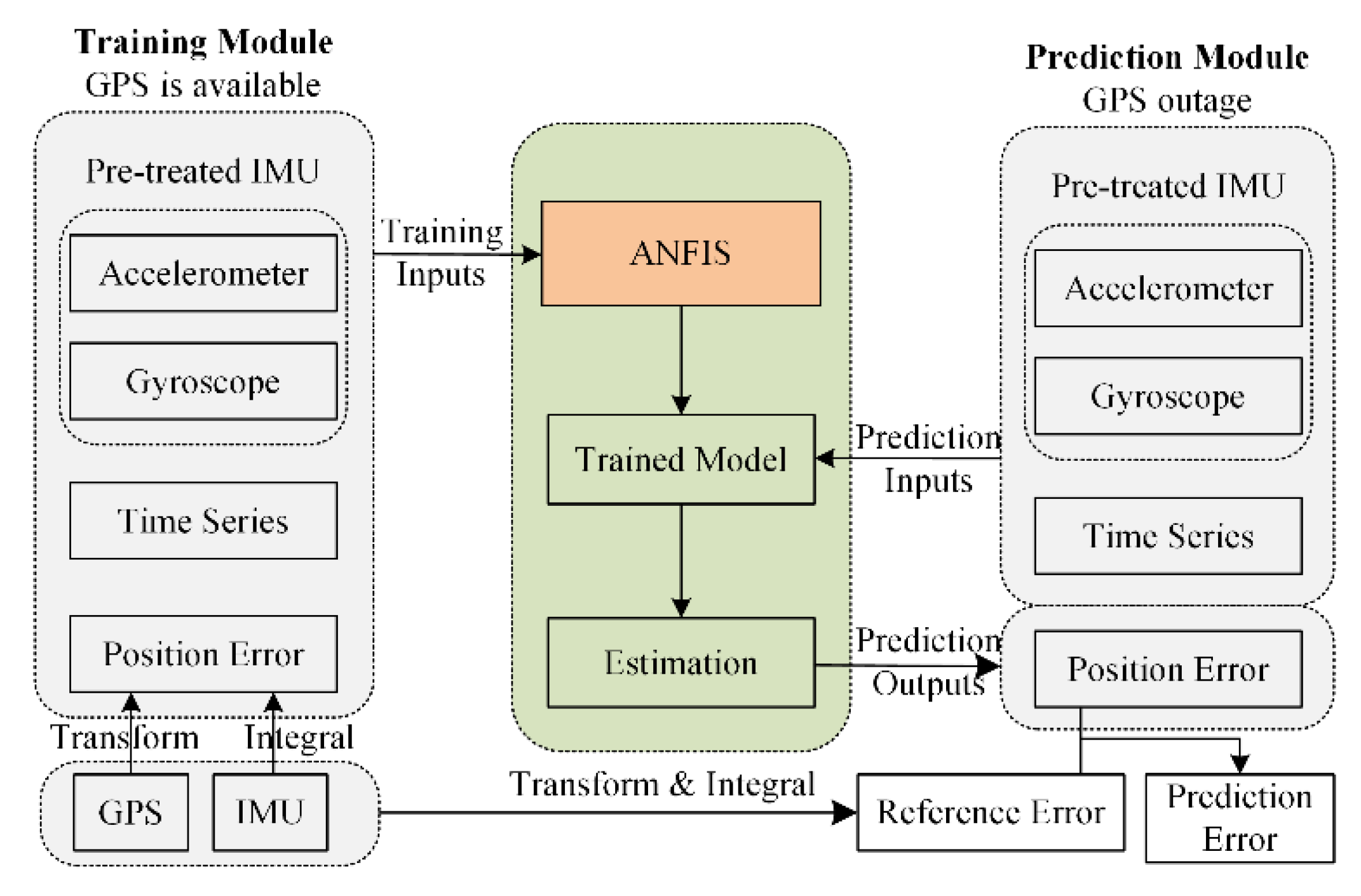
The first ANFIS was proposed in 1993 and has been applied in different fields [45,46,47]. Typical networks contain five layers [48]. The structure of the accumulative error estimation of INS based on an ANFIS designed in this study is shown in Figure 2. The system consists of a training module and a prediction module. The former can be used in open surroundings while the latter is used in covert surroundings. The training module and prediction module errors are obtained from GPS data in this study; alternatively, those errors can be replaced by other sensors such as lidars or cameras in special surroundings. At the training stage, the system inputs are
where the first seven terms on the right-hand side of the equation represent the trained terms denoted by X, and the last two terms represent the target terms denoted by y; the dimension of each term is the number of the training samples; ax, ay, and az are the measured values of accelerometers; gx, gy, and gz are the measured values of gyroscopes; t is the time series; Δx and Δy are the accumulative error of the INS in the b0 system, calculated by
where xtrue and ytrue denote the true position of the vehicle, which can be obtained from precise sensors in suitable surroundings. In this study, the reference position of the vehicle is obtained from differential GPS observations, and ximu and yimu denote and in Equation (10), respectively. After training with the ANFIS, the system obtains a y for each group of X input in the prediction stage.
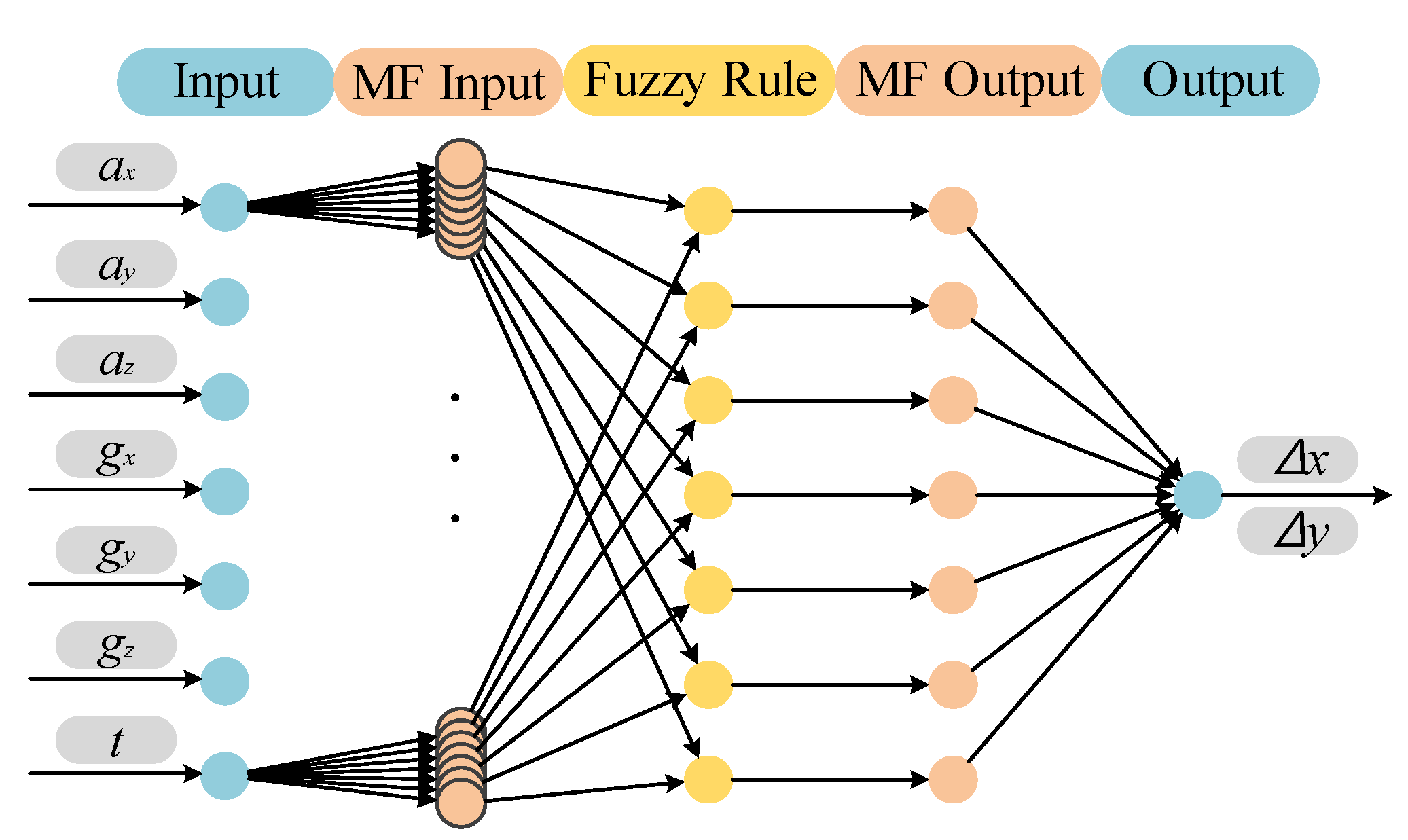
After subtractive clustering is used to generate the Takagi–Sugeno fuzzy inference system [49], the network structure of the algorithm in the accumulative position error estimation of the INS is shown in Figure 3. There are five layers in the network, and the first layer is the input and fuzzification layer. In this study, the Gaussian membership function in Equation (11) was employed to fuzzy the input data. The crisp input value turns to membership degree between 0–1 after fuzzification. The second layer receives the membership degree and applies Equation (13) to calculate the fuzzy factors of each rule. The third layer normalizes the fuzzy factors of each rule through
where m is the number of rules; O3i is the output of the third layer, which represents the trigger weight of rule i in all rules. The results of the fourth layer calculation rule are
where Bi is derived from Equation (12), which is generally a first-order polynomial of the input data; O4i is the output of the fourth layer. The fifth layer outputs the results of the system, using Equation (14) to compute the weighted average of all the rules to defuzzify.
The calculating time of ANFIS is faster than ANN since the BFGS solution mode and FIS generated by subtractive clustering are efficient and rapid.
3. Experiments and Results
Public datasets are utilized for training and predicting one sequence data in different sessions and multi-sequence data. The position error of an INS solution, the position error predicted by the ANN model, and the position error predicted by the ANFIS were compared. Furthermore, LSTM, which is an advanced and improved method based on RNN [11,13,50,51], was compared with ANFIS in the position error prediction.
3.1. Introduction to KITTI
The KITTI dataset was jointly collected by KIT of Germany and TRI-NA, and is currently one of the world’s largest computer vision algorithm evaluation datasets. The sensors include video cameras, laser scanners, GPS, and INS on urban roads, country roads, and expressways [52,53]. The unrectified raw data of GPS and INS in the dataset were used for experiments. Using the IMU data as the observations and the GPS measurements as the reference, the frequency of both observations in the unrectified raw data is 100 Hz.
All data were downloaded from the official website of KITTI. In the downloaded file, the dataformat.txt file contains the GPS and IMU format data, while the timestamps.txt file contains the time stamps. The files under the oxts/data/folder contain all observations, with filenames indicating the data count, and each file contains 30 values. Values-related properties are shown in Table 1. The latitude, longitude, and altitude are the positions in the WGS-84 coordinate system observed by GPS, and the roll, pitch, and yaw are the vehicle attitude angles observed by the gyroscope. The forward acceleration, leftward acceleration, and upward acceleration are the accelerations of the vehicle observed by the accelerometers in the b0 system, and the time stamp is the observation time of the data, which are stored in the timestamps.txt folder.
3.2. Process and Result Analysis
Sequences 20110930_drive_0018 (09300018), 20110930_drive_0033 (09300033), and 20110930_drive_0034 (09300034), which are the unrectified raw data in the residential category, were used in the experiments. The single-sequence position error estimation model was applied based on the 09300018-sequence, and the multi-sequences position error estimation model was employed from three sequences. Some issues were found in that there are repeated observations and missing observations in parts of the unrectified raw observations. To ensure that the observations were not interfered with by humans to a great extent, the processing method included deleting the repeated observations and not interpolating the missing sessions. Since the time stamp file corresponds strictly to the original observation file, the repeated session was also deleted when using the time stamp file.
The positions of the vehicle in the b0 system and the n system were calculated by Equations (4)–(10). The coordinate conversion on the GPS data was simultaneously performed to attain the reference position value of the vehicle in the b0 system and the n system,
where R1, R2 are the rotation matrices, and the specific expression can be referred to as the reference [54,55]. It is stipulated that the X- and Y-directions of the b0 system are the right direction and the forward direction of the initial motion of the vehicle, respectively, while the X- and Y-directions of the n system correspond to the east and north directions of the vehicle. Since the ground truth in the Z-direction has a large error in the KITTI dataset, which can be provided by the observations of the cameras, this study did not consider the motion in the Z-direction.
3.2.1. Single-Sequence Position Error Estimation Model
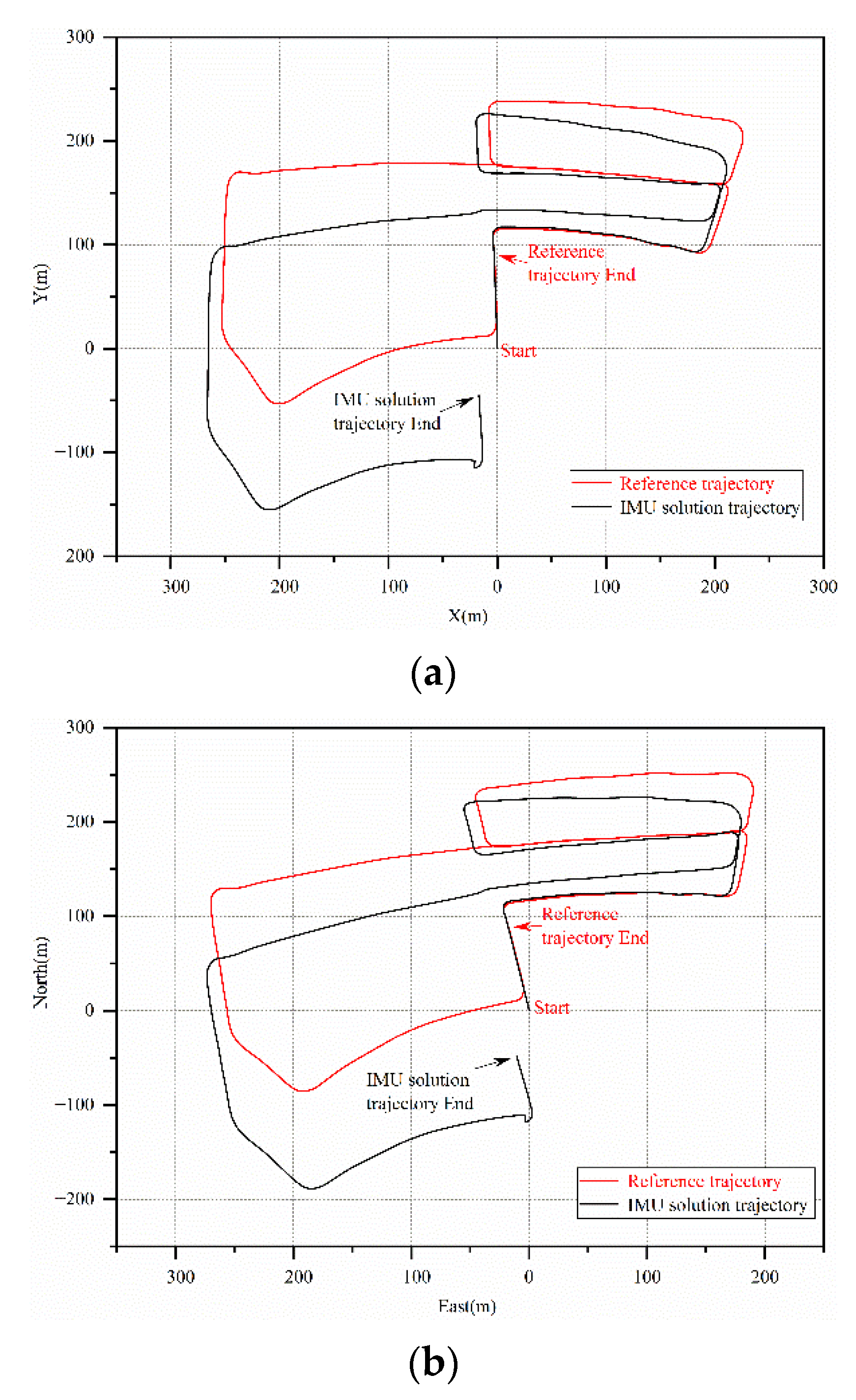
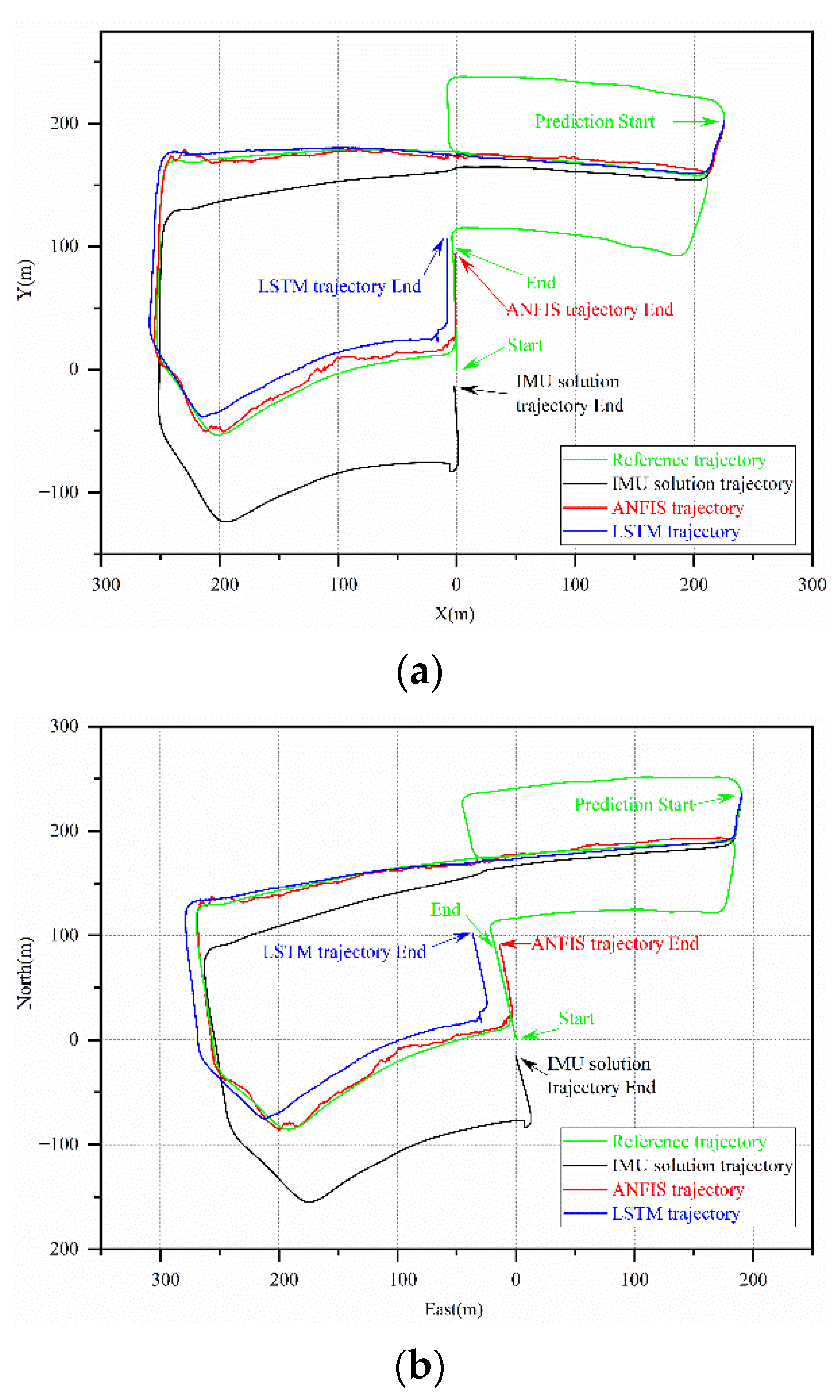
In the 09300018-sequence data, the X-Y trajectory and the east-north trajectory using the INS solution relative to the reference trajectory of the vehicle in the b0 system and the n system are shown in Figure 4a,b, respectively, in which the red line represents the reference trajectory and the black line represents the INS solution trajectory. The track discontinuity is the missing observations session after deleting the IMU repeated observations. It can be seen from Figure 4 that, due to the accumulative position error of INS, the INS solution trajectory is distinct from the reference trajectory, and the difference between the two trajectories at the end point is 135.65 m.
In this study, the strategy of using ANFIS, ANN, and LSTM for single-sequence position error estimation is to use half of the total observations as the training sample to predict the position error of the other half of the observations, and contrast the accuracy of the three models for accumulative position error prediction of the INS in the b0 system and the n system, respectively. The data of the training part represent the moment where GPS is available, and the data of the prediction part simulate the vehicle in complex and covert surroundings.
In the training stage, subtractive clustering is used to generate FIS. Using the training data and the corresponding reference data as the input and setting some parameters, the ANFIS structure can be built. In addition, the parameters which include the optimization method, the maximum epoch, the error goal, and the initial step size should be identified. Digitals of the trained model by using ANFIS and LSTM in this experiment can be found at: https://github.com/robNavLoc/IMU-error-prediction-based-on-ANFIS (accessed on 31 May 2021). Training results are shown in Table 2. It can be seen that, due to the fuzzy logical system, the training results of the ANFIS are better than the results of the LSTM.
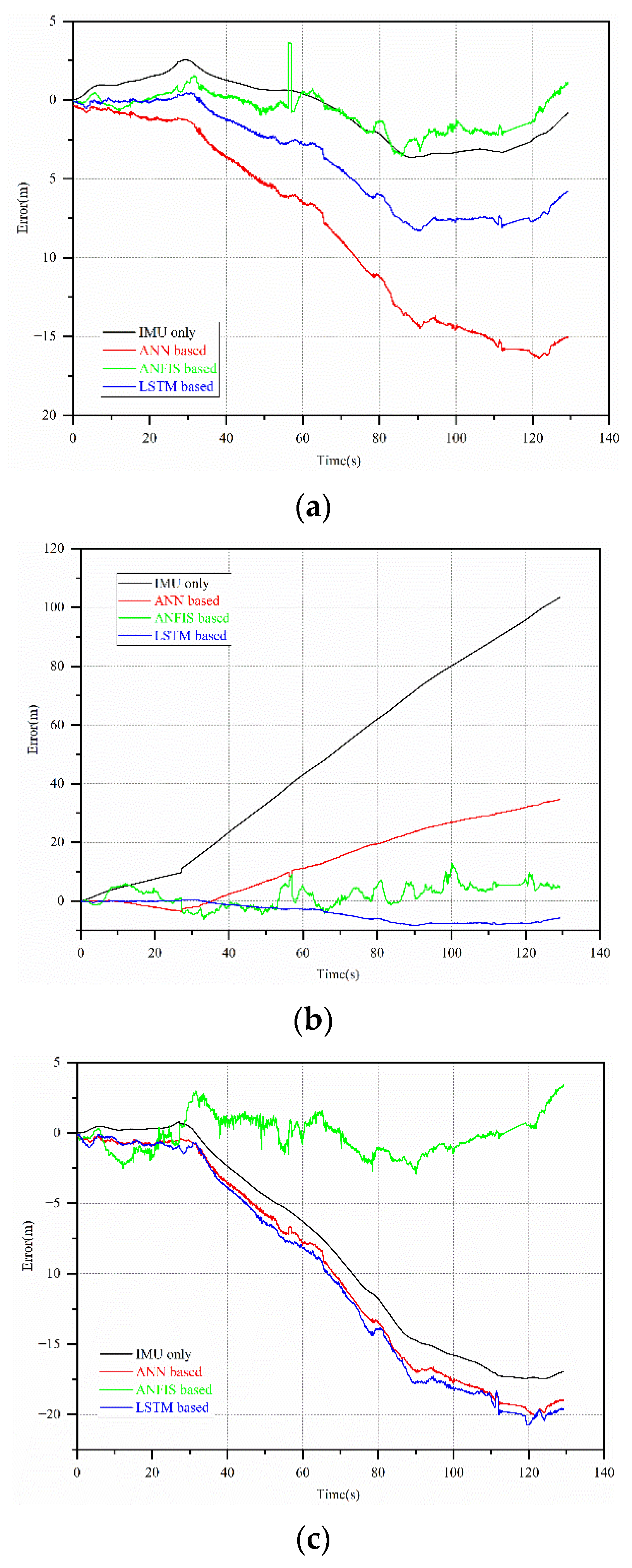
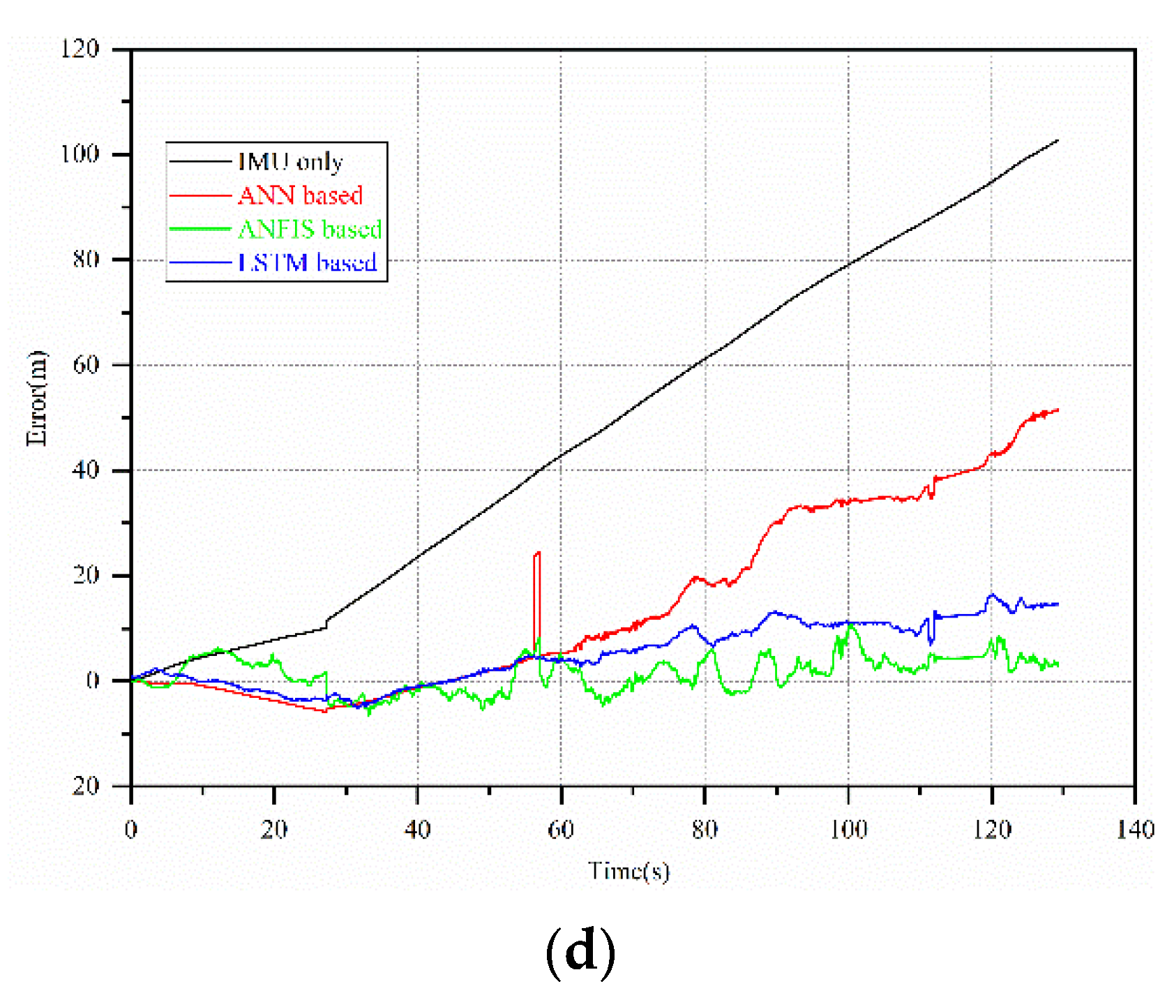
In the prediction stage, the vehicle runs 1052.9 m in 129.31 s. The position error estimated by the ANN, ANFIS, LSTM, and the INS solution versus time is shown in Figure 5. The green line, blue line, red line, and black line represent the accumulative position error of the ANFIS model, the LSTM model, the ANN model, and INS solution, respectively. Figure 5a–d exhibit the prediction position error in X-direction, Y-direction, east direction, and north direction, respectively. The mean square error (MSE), the root mean square error (RMSE), and the accumulative position error of each curve shown in Figure 5 in the b0 system and the n system are shown in Table 3 and Table 4, respectively.
Figure 5a,b shows that the vehicle’s error in the Y-direction was much higher than in the X-direction. When the ANN model and LSTM model were used to predict and correct the accumulative position error of INS, they showed the effective result in the Y-direction, but the position errors in the X-direction were larger, which may be caused by the insufficient training samples of the ANN model. ANFIS performs far better than the ANN model in the X- and Y-directions and virtually restored the true position of the vehicle. Similar results can be seen in Figure 5c,d that ANFIS had a smaller predicting error than the INS solution and ANN. Moreover, the prediction accuracy of ANFIS is better than LSTM.
As seen from Table 3 and Table 4, to a certain extent, ANN improved the Y-direction and north direction accuracy, and MSE was decreased to 10.3% and 16.1% of the position error, respectively, but it increased the X-direction and the east direction errors. In total, the accumulative errors decreased from 9.83% to 3.59% and 5.34% in the b0 and the n systems, respectively. Similar to the ANN, the LSTM decreased the error of the Y-direction and increased the X-direction, which ultimately results in a reduction in error from 9.83% to 1.77% and 2.33% in the b0 system and the n systems, respectively. Compared with the ANN, the LSTM, and the INS solution, the error predicted by the ANFIS was lower. Compared with the INS solution, the RMSE in the X-direction and the east direction using ANFIS was reduced to 65.4% and 12.3%, respectively, and the RMSE of the Y-direction and the north direction using ANFIS was correspondingly reduced to 7.1% and 6.3%, respectively. Overall, the accumulative errors were reduced from 9.83% to 0.45% and 0.43% in the b0 and the n systems, respectively. It shows that the vehicle trajectory obtained by ANFIS has a superior fitting degree with the reference trajectory.
By comprehensively comparing Figure 5a–d and Table 3 and Table 4, the results calculated by ANN and LSTM in the b0 system are better than those in the n system. This was due to the SINS being installed on the vehicle and observations being attained from the sensors in the b system. However, this conclusion is not apparent when using ANFIS, so the following experiment only show the results under the b0 system.
The reference trajectory of the vehicle, the trajectory corrected by the ANFIS, and the INS solution trajectory of the corresponding time are shown in Figure 6, where Figure 6a,b shows the vehicle trajectories of the b0 and n systems, respectively. It can be seen that ANFIS performed well in the estimation of the accumulative position error of INS, which largely corrects the vehicle position deviation caused by the accumulative position error of INS.
3.2.2. Multi-Sequences Position Error Estimation Model
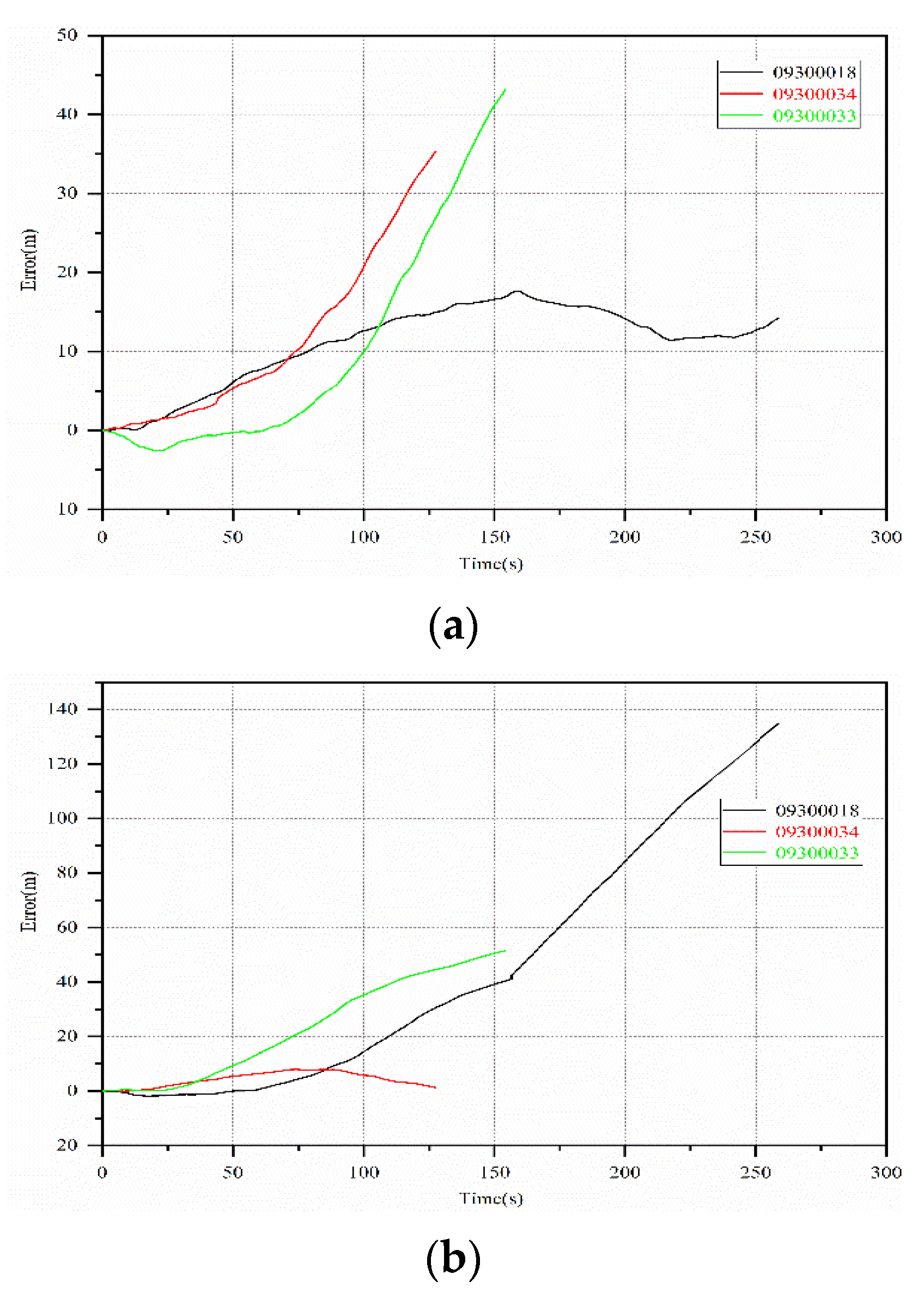
The error accumulation curves of sequences 09300018, 09300033, 09300034 in the b0 system are shown in Figure 7, where Figure 7a,b shows the error accumulation curve in the X- and Y-directions, respectively. The black, red, and green lines indicate the 09300018, 09300033, 09300034 curves, respectively. The information of each sequence is shown in Table 5. As shown in Figure 7 and Table 5, the accumulation of each curve of error over time between curves shows different change trends, but they were gradually increasing overall, and the accumulative position error in each sequence has some correlation with the driving time; thus, the position error of an entire sequence could be predicted by similar sequences [18].
In this study, the strategy of using ANFIS for multi-sequences error estimation is to use the 09300018 and 09300034 observations and errors as training samples to predict the error of the 09300033 observations and compare the error prediction accuracy of the INS solution and the ANFIS in the b0 system. Similarly, the data of the training part represent the moment when the GPS is available, and the data of the prediction part simulate the vehicle in complex and covert surroundings.
Similar to the single-sequence, the subtractive clustering method was also used in the multi-sequences experiment to generate FIS, and then the training data and reference data were used to generate the training model. As the time series were included in the training inputs, the data of the sequences can be shuffled to satisfy randomness. Digitals of the trained model in this experiment can be found on the same website.
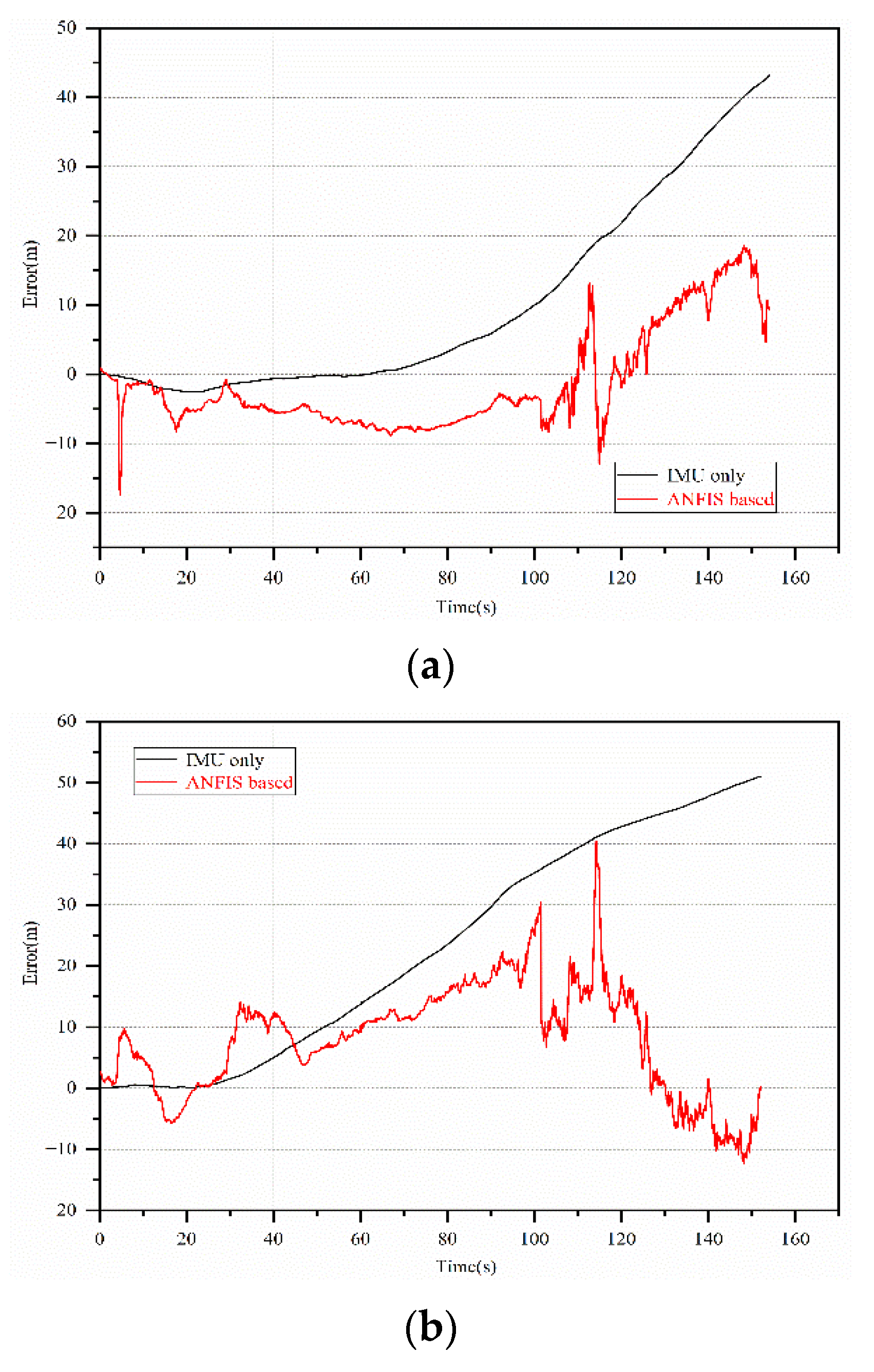
In the prediction stage, the driven time and distance of the vehicle in each sequence are shown in Table 5. The curve of the position error predicted by ANFIS and calculated by IMU is shown in Figure 8. The red line and black line represent the predicted position error of the INS by using the ANFIS model and the INS solution, respectively. Figure 8a,b shows the error in the X- and Y-directions in the b0 system of the vehicle, respectively. The mean square error (MSE), the root mean square error (RMSE), and the accumulative error of each trajectory in the b0 system were calculated as shown in Table 6.
It can be seen from Figure 8a,b that the accumulative position error of INS increased sharply over time, while the ANFIS error did not show a cumulative trend. In the initial stage of vehicle moving, ANFIS did not perform well in predicting errors due to the low INS solution error in the initial stage and the weak correlation of the error in the different road sections, leading to the fluctuation of ANFIS error prediction. Between 100–120 s of vehicle moving, the findings were not ideal because of the complex road conditions. However, overall, ANFIS could correct the accumulative position error of INS to a large extent. It can be seen from Table 6, compared to the INS solution, the MSE of the ANFIS algorithm in the X- and Y-directions was greatly decreased, and the accumulative error w was decreased from 4.1% to 0.6%.
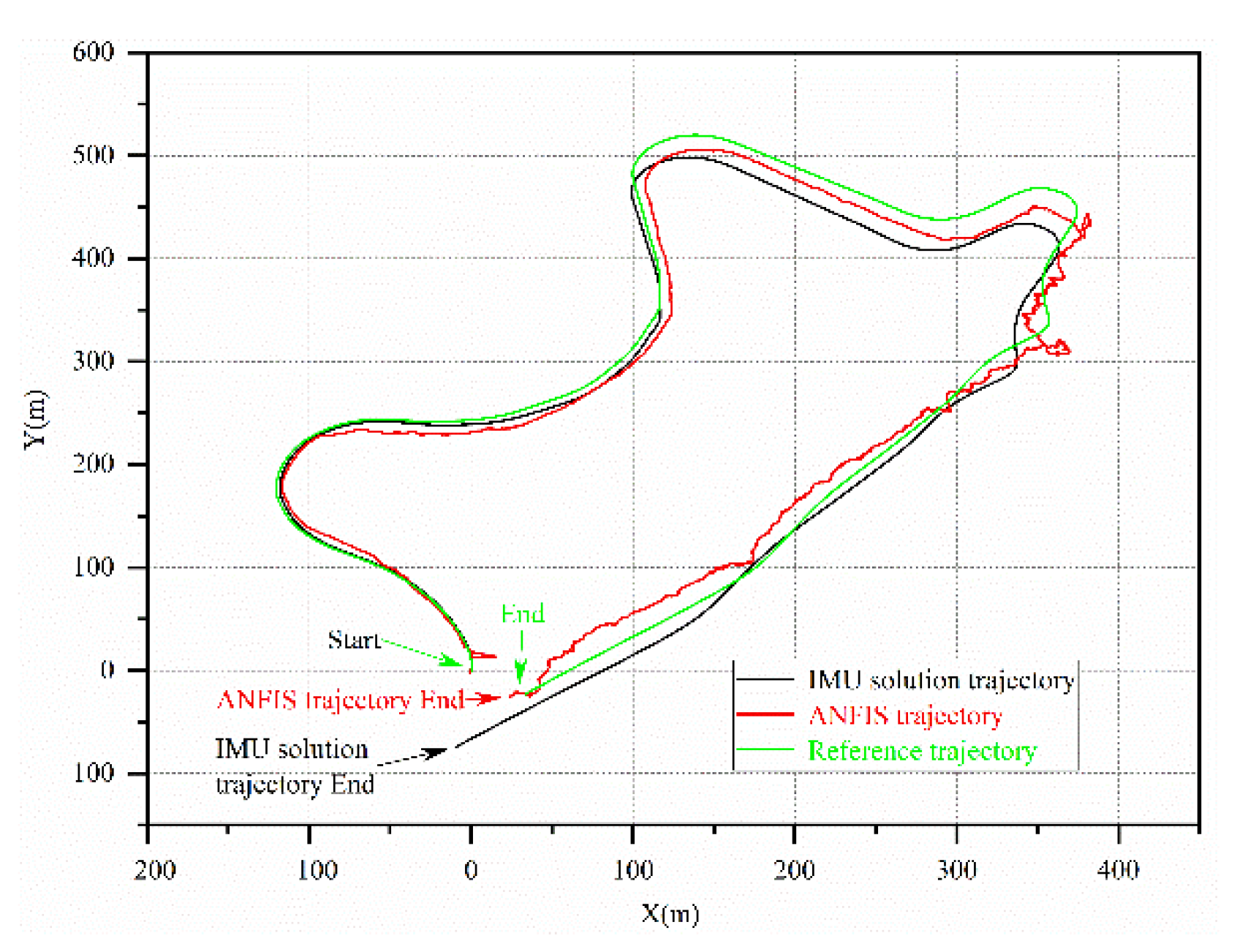
The reference trajectory of the vehicle, the trajectory corrected by the ANFIS estimation INS solution error, and the INS solution trajectory of the corresponding time are shown in Figure 9.
Through the above two experiments, a single-sequence can predict the accumulative position error of INS more accurately because of its continuity of motion, which almost restores the true location information of the vehicle. Due to the independent observation of each road section in multi-sequences, the correlation of the error of the INS at the initial stage was weak and had a high error. After a long driving period, the error of the INS in different road sections was strongly correlated, and the error was decreased.
4. Discussion
The results showed that the proposed ANFIS effectively reduced the position error of the vehicle in the single-sequence experiment and multi-sequences experiment. However, because fewer sequences were used, the result of the multi-sequences experiment did not perform as well as using CNN [18].
The trajectory in an upward direction was not considered in the experiments because the ground truth provided by the KITTI dataset occasionally had large errors in the Z-direction. Future work will involve training a model by using other datasets and collect data under more difficult conditions.
The LSTM method decreased the position error to a large extent but did not perform as well as ANFIS. The reason may be that the vehicle stopped for a few seconds, breaking the continuity of the time-series problem.
Due to the small INS solution error in the initial stage of the multi sequences experiment, the error predicted by ANFIS was often higher than that of the INS solution error at this stage, and the effect was worse on the road section with more bends. To address this, future work should adjust the input values of the ANFIS model in the initial stage and increase the training set of winding roads.
5. Conclusions
In this study, a model for estimating the accumulative position error of the INS based on ANFIS, which can quickly and accurately output the position error of a vehicle end-to-end, is proposed. The new system was employed to estimate and correct the accumulative position error of the INS to obtain the accurate position information of a vehicle in complex and covert surroundings where other sensors do not work consistently. The proposed method was verified using the KITTI dataset, and results indicated that the accumulative position error was decreased to 0.45% and 0.61% in single-sequence and multi-sequences experiments by using ANFIS, respectively; this was significantly less than those of the other three approaches. This result suggests that the ANFIS could considerably improve the positioning accuracy of inertial navigation, which has significance for vehicle inertial navigation in complex and covert surroundings.
Author Contributions
Conceptualization, Yabo Duan and Huaizhan Li; methodology, Yabo Duan; software, Yabo Duan; validation, Huaizhan Li, Kefei Zhang and Suqin Wu; formal analysis, Yabo Duan; investigation, Huaizhan Li; resources, Kefei Zhang; data curation, Yabo Duan; writing—original draft preparation, Yabo Duan; writing—review and editing, Suqin Wu and Huaizhan Li; visualization, Huaizhan Li; supervision, Huaizhan Li; project administration, Kefei Zhang; funding acquisition, Kefei Zhang. All authors have read and agreed to the published version of the manuscript.
Funding
This work was funded by the State Key Program of National Natural Science Foundation of China, Grant No. 41730109; National Natural Science Foundation of China, grant number 51804301; Programme of Introducing Talents of Discipline to Universities, Grant No. B20046; Independent Innovation Project of “Double-First Class” Construction, grant number 2018ZZCX08; Natural Science Foundation of Jiangsu Province, grant number BK20180661; and Postdoctoral Science Foundation, grant number 2019M660135. We would like to acknowledge the support of the Jiangsu dual creative talents and Jiangsu dual creative team’s programme projects, awarded in 2017.
Institutional Review Board Statement
Not applicable.
Informed Consent Statement
Not applicable.
Data Availability Statement
The data supporting reported results can be found at https://github.com/robNavLoc/IMU-error-prediction-based-on-ANFIS, accessed on 4 June 2021.
Conflicts of Interest
The authors declare no conflict of interest.
References
- Franz, M.O.; Mallot, H.A. Biomimetic robot navigation. Robot. Auton. Syst. 2000, 30, 133–153. [Google Scholar] [CrossRef] [Green Version]
- Shaeffer, D.K. MEMS inertial sensors: A tutorial overview. IEEE Commun. Mag. 2013, 51, 100–109. [Google Scholar] [CrossRef]
- Leung, K.T.; Whidborne, J.F.; Purdy, D.; Dunoyer, A. A review of ground vehicle dynamic state estimations utilising GPS/INS. Veh. Syst. Dyn. 2011, 49, 29–58. [Google Scholar] [CrossRef]
- Yassin, A.; Nasser, Y.; Awad, M.; Al-Dubai, A.; Liu, R.; Yuen, C.; Raulefs, R.; Aboutanios, E. Recent Advances in Indoor Localization: A Survey on Theoretical Approaches and Applications. IEEE Commun. Surv. Tutor. 2017, 19, 1327–1346. [Google Scholar] [CrossRef] [Green Version]
- Paull, L.; Saeedi, S.; Seto, M.; Li, H. AUV Navigation and Localization: A Review. IEEE J. Ocean. Eng. 2014, 39, 131–149. [Google Scholar] [CrossRef]
- Shaukat, A.; Blacker, P.; Spiteri, C.; Gao, Y. Towards Camera-LIDAR Fusion-Based Terrain Modelling for Planetary Surfaces: Review and Analysis. Sensors 2016, 16, 1952. [Google Scholar] [CrossRef] [Green Version]
- Sharaf, R.; Noureldin, A.; Osman, A.; El-Sheimy, N. Online INS/GPS integration with a radial basis function neural network. IEEE Aerosp. Electron. Syst. Mag. 2005, 20, 8–14. [Google Scholar] [CrossRef]
- Noureldin, A.; El-Shafie, A.; Bayoumi, M. GPS/INS integration utilizing dynamic neural networks for vehicular navigation. Inf. Fusion 2011, 12, 48–57. [Google Scholar] [CrossRef]
- El Shafie, A.; Hussain, A.; Eldin, A.E.N. ANFIS-Based Model for Real-time INS/GPS Data Fusion for Vehicular Navigation System. In Proceedings of the 2009 International Conference on Computer Technology and Development, Kota Kinabalu, Malaysia, 13–15 November 2009; Volume 2. [Google Scholar]
- Du, S.; Gan, X.; Zhang, R.; Zhou, Z. The Integration of Rotary MEMS INS and GNSS with Artificial Neural Networks. Math. Probl. Eng. 2021, 2021. [Google Scholar] [CrossRef]
- Brossard, M.; Bonnabel, S. Learning wheel odometry and IMU errors for localization. In Proceedings of the 2019 International Conference on Robotics and Automation (ICRA), Montreal, QC, Canada, 20–24 May 2019. [Google Scholar]
- Chen, D.; Han, J.Q. Application of wavelet neural network in signal processing of MEMS accelerometers. Microsyst. Technol. 2011, 17, 1–5. [Google Scholar] [CrossRef]
- Jiang, C.H.; Chen, S.; Chen, Y.W.; Zhang, B.; Feng, Z.; Zhou, H.; Bo, Y. A MEMS IMU de-noising method using long short-term memory recurrent neural networks (LSTM-RNN). Sensors 2018, 18, 3470. [Google Scholar] [CrossRef] [PubMed] [Green Version]
- Li, Q.; Ben, Y.; Sun, F. Strapdown fiber optic gyrocompass using adaptive network-based fuzzy inference system. Opt. Eng. 2014, 53, 014103. [Google Scholar] [CrossRef]
- Kaygisiz, B.H.; Erkmen, I.; Erkmen, A.M. GPS/INS Enhancement for Land Navigation using Neural Network. J. Navig. 2004, 57, 297–310. [Google Scholar] [CrossRef]
- Srinivasan, S.; Sa, I.; Zyner, A.; Reijgwart, V.; Siegwart, R. End-to-end velocity estimation for autonomous racing. IEEE Robot. Autom. Lett. 2020, 5, 6869–6875. [Google Scholar] [CrossRef]
- Lima, J.P.S.D.; Uchiyama, H.; Taniguchi, R. End-to-End Learning Framework for IMU-Based 6-DOF Odometry. Sensors 2019, 19, 3777. [Google Scholar] [CrossRef] [Green Version]
- Brossard, M.; Barrau, A.; Bonnabel, S. AI-IMU Dead-Reckoning. IEEE Trans. Intell. Veh. 2020, 5, 585–595. [Google Scholar] [CrossRef]
- Yan, H.; Shan, Q.; Furukawa, Y. RIDI: Robust IMU double integration. In Proceedings of the 15th European Conference on Computer Vision (ECCV), Munich, Germany, 8–14 September 2018. [Google Scholar]
- Chen, X.; Shen, C.; Zhang, W.; Tomizuka, M.; Xu, Y.; Chiu, K. Novel hybrid of strong tracking Kalman filter and wavelet neural network for GPS/INS during GPS outages. Measurement 2013, 46, 3847–3854. [Google Scholar] [CrossRef]
- Yang, Y.; Zhong, Y.; Gao, Y. Model predictive filter based neural networks for INS/GPS integrated navigation during GPS outages. In Proceedings of the 2017 IEEE 7th International Conference on Electronics Information and Emergency Communication (ICEIEC), Macau, China, 21–23 July 2017. [Google Scholar]
- Adusumilli, S.; Bhatt, D.; Wang, H.; Bhattacharya, P.; Devabhaktuni, V. A low-cost INS/GPS integration methodology based on random forest regression. Expert Syst. Appl. 2013, 40, 4653–4659. [Google Scholar] [CrossRef]
- Jaradat, M.A.; Abdel-Hafez, M.F.; Saadeddin, K.; Jarrah, M.A. Intelligent fault detection and fusion for INS/GPS navigation system. In Proceedings of the 9th International Symposium on Mechatronics and its Applications (ISMA), Amman, Jordan, 9–11 April 2013. [Google Scholar]
- Grigorie, L.T.; Jula, N.; Corcau, C.L.; Adochiei, I.R.; Larco, C.; Mustaţă, S.M. A positioning mechanism based on MEMS-INS/GPS and ANFIS data fusion for urban life mobility improvement. In Proceedings of the 4th International Conference on Nanotechnologies and Biomedical Engineering (ICNBME), Chisinau, Moldova, 18–21 September 2019. [Google Scholar]
- Abdel-Hamid, W.; Noureldin, A.; El-Sheimy, N. Adaptive fuzzy prediction of low-cost inertial-based positioning errors. IEEE Trans. Fuzzy Syst. 2007, 15, 519–529. [Google Scholar] [CrossRef]
- Jaradat, M.A.K.; Abdel-Hafez, M.F. Enhanced, delay dependent, intelligent fusion for INS/GPS navigation system. IEEE Sens. J. 2014, 14, 1545–1554. [Google Scholar] [CrossRef]
- Saadeddin, K.; Abdel-Hafez, M.F.; Jaradat, M.A.; Jarrah, M.A. Optimization of intelligent approach for low-cost INS/GPS navigation system. J. Intell. Robot. Syst. 2014, 73, 325–348. [Google Scholar] [CrossRef]
- Abdolkarimi, E.S.; Mosavi, M.R. Wavelet-adaptive neural subtractive clustering fuzzy inference system to enhance low-cost and high-speed INS/GPS navigation system. GPS Solut. 2020, 24. [Google Scholar] [CrossRef]
- Saadeddin, K.; Abdel-Hafez, M.F.; Jaradat, M.A.; Jarrah, M.A. Performance enhancement of low-cost, high-accuracy, state estimation for vehicle collision prevention system using ANFIS. Mech. Syst. Signal Process. 2013, 41, 239–253. [Google Scholar] [CrossRef]
- Wu, Y.; Hu, X.; Hu, D.; Li, T.; Lian, J. Strapdown inertial navigation system algorithms based on dual quaternions. IEEE Trans. Aerosp. Electron. Syst. 2005, 41, 110–132. [Google Scholar] [CrossRef]
- Stamou, G.B.; Tzafestas, S.G. Fuzzy relation equations and fuzzy inference systems: An inside approach. IEEE Trans. Syst. Man Cybernetics Part B Cybern. 1999, 29, 694–702. [Google Scholar] [CrossRef]
- Son, L.H.; Van Viet, P.; Van Hai, P. Picture inference system: A new fuzzy inference system on picture fuzzy set. Appl. Intell. 2017, 46, 652–669. [Google Scholar] [CrossRef]
- Schott, D.J.; Hoflinger, F.; Zhang, R.; Reindl, L.M.; Yang, H. Fuzzy inference system assisted inertial localization system. In Proceedings of the 2017 International Conference on Engineering, Technology and Innovation (ICE/ITMC), Madeira, Portugal, 27–29 June 2017. [Google Scholar]
- Wang, L.X. A Course in Fuzzy Systems and Control; Prentice-Hall: Hoboken, NJ, USA, 1997; pp. 90–149. ISBN 978-01-3540-882-7. [Google Scholar]
- Chung-Shi, T.; Bor-Sen, C.; Huey-Jian, U. Fuzzy tracking control design for nonlinear dynamic systems via T-S fuzzy model. IEEE Trans. Fuzzy Syst. 2001, 9, 381–392. [Google Scholar] [CrossRef] [Green Version]
- Basheer, I.A.; Hajmeer, M. Artificial neural networks: Fundamentals, computing, design, and application. J. Microbiol. Methods 2000, 43, 3–31. [Google Scholar] [CrossRef]
- Schmidhuber, J. Deep learning in neural networks: An overview. Neural Netw. 2015, 61, 85–117. [Google Scholar] [CrossRef] [PubMed] [Green Version]
- Plumb, A.P.; Rowe, R.C.; York, P.; Brown, M. Optimisation of the predictive ability of artificial neural network (ANN) models: A comparison of three ANN programs and four classes of training algorithm. Eur. J. Pharm. Sci. 2005, 25, 395–405. [Google Scholar] [CrossRef]
- Che, Z.; Chiang, T.; Che, Z. Feed-forward neural networks training: A comparison between genetic algorithm and back-propagation learning algorithm. Int. J. Innov. Comput. Inf. Control. 2011, 7, 5839–5850. [Google Scholar] [CrossRef]
- Zhang, Y.; Mu, B.; Zheng, H. Link Between and Comparison and Combination of Zhang Neural Network and Quasi-Newton BFGS Method for Time-Varying Quadratic Minimization. IEEE Trans. Cybern. 2013, 43, 490–503. [Google Scholar] [CrossRef]
- Xu, Q.; Zhang, C.; Zhang, L.; Song, Y. The Learning Effect of Different Hidden Layers Stacked Autoencoder. In Proceedings of the 2016 8th International Conference on Intelligent Human-Machine Systems and Cybernetics (IHMSC), Hangzhou, China, 11–12 September 2016; Volume 2. [Google Scholar]
- Mirchandani, G.; Cao, W. On hidden nodes for neural nets. IEEE Trans. Circuits Syst. 1989, 36, 661–664. [Google Scholar] [CrossRef]
- Wanas, N.; Auda, G.; Kamel, M.S.; Karray, F.A.K.F. On the optimal number of hidden nodes in a neural network. In Proceedings of the IEEE Canadian Conference on Electrical and Computer Engineering (Cat. No.98TH8341), Waterloo, ON, Canada, 25–28 May 1998; Volume 1–2. [Google Scholar]
- Kuo, R.J.; Chen, C.H.; Hwang, Y.C. An intelligent stock trading decision support system through integration of genetic algorithm based fuzzy neural network and artificial neural network. Fuzzy Sets Syst. 2001, 118, 21–45. [Google Scholar] [CrossRef]
- Pradhan, B. A comparative study on the predictive ability of the decision tree, support vector machine and neuro-fuzzy models in landslide susceptibility mapping using GIS. Comput. Geosci. 2013, 51, 350–365. [Google Scholar] [CrossRef]
- Nayak, P.C.; Sudheer, K.P.; Rangan, D.M.; Ramasastri, K.S. A neuro-fuzzy computing technique for modeling hydrological time series. J. Hydrol. 2004, 291, 52–66. [Google Scholar] [CrossRef]
- Suganthi, L.; Iniyan, S.; Samuel, A.A. Applications of fuzzy logic in renewable energy systems—A review. Renew. Sustain. Energy Rev. 2015, 48, 585–607. [Google Scholar] [CrossRef]
- Jang, R.J. ANFIS: Adaptive-network-based fuzzy inference system. IEEE Trans. Syst. Man Cybern. 1993, 23, 665–685. [Google Scholar] [CrossRef]
- Lohani, A.K.; Goel, N.K.; Bhatia, K.K.S. Takagi–Sugeno fuzzy inference system for modeling stage–discharge relationship. J. Hydrol. 2006, 331, 146–160. [Google Scholar] [CrossRef]
- Zhang, M.; Zhang, M.; Chen, Y.; Li, M. IMU data processing for inertial aided navigation: A recurrent neural network based approach. In Proceedings of the IEEE International Conference on Robotics and Automation (ICRA), Xian, China, 31 May–5 June 2021. [Google Scholar]
- Podobnik, J.; Kraljic, D.; Zadravec, M.; Munih, M. Centre of pressure estimation during walking using only inertial-measurement units and end-to-end statistical modelling. Sensors 2020, 20, 6136. [Google Scholar] [CrossRef]
- Geiger, A.; Lenz, P.; Stiller, C.; Urtasun, R. Vision meets robotics: The KITTI dataset. Int. J. Robot. Res. 2013, 32, 1231–1237. [Google Scholar] [CrossRef] [Green Version]
- Geiger, A.; Lenz, P.; Urtasun, R. Are we ready for Autonomous Driving? The KITTI Vision Benchmark Suite. In Proceedings of the 2012 IEEE Conference on Computer Vision and Pattern Recognition (CVPR), Providence, RI, USA, 16–21 June 2012. [Google Scholar]
- Farrell, J.A.; Barth, M. The Global Positioning System and Inertial Navigation; McGraw-Hill: New York, NY, USA, 1999; pp. 21–28. ISBN 007022045X. [Google Scholar]
- MathWorks. 3-D Coordinate and Vector Transformations—Functions. 2021. Available online: https://www.mathworks.com/help/map/referencelist.html?type=function&category=3-d-coordinate-and-vector-transformations&s_tid=CRUX_topnav (accessed on 26 May 2021).
Figure 1.
Structure of a fuzzy inference system.

Figure 2.
Structure of the accumulative error estimation of INS based on an ANFIS.

Figure 3.
Network structure of ANFIS.

Figure 4.
Reference trajectory and INS solution trajectory: (a) trajectory in b0 system; (b) trajectory in the n system.
Figure 4.
Reference trajectory and INS solution trajectory: (a) trajectory in b0 system; (b) trajectory in the n system.

Figure 5.
Error accumulation curve of three algorithms: (a) X-direction position error in the b0 system; (b) Y-direction position error in the b0 system; (c) east direction position error in the n system; (d) north direction position error in the n system.
Figure 5.
Error accumulation curve of three algorithms: (a) X-direction position error in the b0 system; (b) Y-direction position error in the b0 system; (c) east direction position error in the n system; (d) north direction position error in the n system.


Figure 6.
Comparison of INS solution trajectory, ANFIS trajectory, and true trajectory: (a) trajectory in the b0 system; (b)trajectory in the n system.
Figure 6.
Comparison of INS solution trajectory, ANFIS trajectory, and true trajectory: (a) trajectory in the b0 system; (b)trajectory in the n system.

Figure 7.
Cumulative error curve of three sequences: (a) X direction position error; (b) Y direction position error.
Figure 7.
Cumulative error curve of three sequences: (a) X direction position error; (b) Y direction position error.

Figure 8.
Error accumulation curve of two algorithms: (a) X-direction position error; (b) Y-direction position error.
Figure 8.
Error accumulation curve of two algorithms: (a) X-direction position error; (b) Y-direction position error.

Figure 9.
Comparison of INS solution trajectory, ANFIS trajectory and true trajectory.


Table 1.
Attribute related to values used. LIF means the list of the value in the file.
| Value | Unit | LIF | Remarks |
|---|---|---|---|
| Latitude | deg | 1 | WGS-84 |
| Longitude | deg | 2 | |
| Altitude | m | 3 | |
| Roll | rad | 4 | (−π–π) |
| Pitch | rad | 5 | (−1/2π–1/2π) |
| Yaw | rad | 6 | (−π–π) |
| Forward acceleration | m/s2 | 12 | b system |
| Leftward acceleration | m/s2 | 13 | |
| Upward acceleration | m/s2 | 14 | |
| Time stamp | s | / | timestamp.txt |
Table 2.
Training results of the LSTM and ANFIS methods.
| LSTM | ANFIS | |||||||
|---|---|---|---|---|---|---|---|---|
| Direction | X | Y | East | North | X | Y | East | North |
| MSE | 0.00045 | 3.9 | 0.09 | 2.9 | 0.0017 | 0.0079 | 0.0039 | 0.0088 |
| RMSE | 0.02 | 1.97 | 0.30 | 1.70 | 0.04 | 0.09 | 0.06 | 0.09 |
Table 3.
Error statistics of three algorithms in the b0 system.
| IMU Solution | ANN | LSTM | ANFIS | |||||
|---|---|---|---|---|---|---|---|---|
| X | Y | X | Y | X | Y | X | Y | |
| MSE | 4.46 | 3351.00 | 100.15 | 345.45 | 25.19 | 109.86 | 1.90 | 16.85 |
| RMSE | 2.11 | 57.89 | 10.01 | 18.59 | 5.02 | 10.48 | 1.38 | 4.11 |
| Accumulative Error | 9.83% | 3.59% | 1.77% | 0.45% | ||||
| Distance | 1052.9 m | |||||||
Table 4.
Error statistics of three algorithms in the n system.
| IMU Solution | ANN | LSTM | ANFIS | |||||
|---|---|---|---|---|---|---|---|---|
| East | North | East | North | East | North | East | North | |
| MSE | 113.67 | 3280.96 | 145.43 | 529.14 | 155.43 | 62.23 | 1.71 | 13.16 |
| RMSE | 10.66 | 57.28 | 12.06 | 23.00 | 12.47 | 7.89 | 1.31 | 3.63 |
| Accumulative Error | 9.83% | 5.34% | 2.33% | 0.43% | ||||
| Distance | 1052.9 m | |||||||
Table 5.
Information of each sequence.
| Sequence | Driving Time/s | Driving Distance/m | Accumulative Error |
|---|---|---|---|
| 09300018 | 260.29 | 1925.87 | 7.04% |
| 09300033 | 154.07 | 1623.47 | 4.14% |
| 09300034 | 127.53 | 919.89 | 3.84% |
Table 6.
Error statistics of two algorithms.
| IMU Solution | ANFIS | |||
|---|---|---|---|---|
| X | Y | X | Y | |
| MSE | 288.33 | 865.53 | 54.25 | 143.41 |
| RMSE | 16.98 | 29.42 | 7.37 | 11.98 |
| Accumulative Error | 4.14% | 0.61% | ||
| Distance | 1623.47 m | |||
Publisher’s Note: MDPI stays neutral with regard to jurisdictional claims in published maps and institutional affiliations. |
© 2021 by the authors. Licensee MDPI, Basel, Switzerland. This article is an open access article distributed under the terms and conditions of the Creative Commons Attribution (CC BY) license (https://creativecommons.org/licenses/by/4.0/).
Share and Cite
MDPI and ACS Style
Duan, Y.; Li, H.; Wu, S.; Zhang, K. INS Error Estimation Based on an ANFIS and Its Application in Complex and Covert Surroundings. ISPRS Int. J. Geo-Inf. 2021, 10, 388. https://0-doi-org.brum.beds.ac.uk/10.3390/ijgi10060388
AMA Style
Duan Y, Li H, Wu S, Zhang K. INS Error Estimation Based on an ANFIS and Its Application in Complex and Covert Surroundings. ISPRS International Journal of Geo-Information. 2021; 10(6):388. https://0-doi-org.brum.beds.ac.uk/10.3390/ijgi10060388
Chicago/Turabian StyleDuan, Yabo, Huaizhan Li, Suqin Wu, and Kefei Zhang. 2021. "INS Error Estimation Based on an ANFIS and Its Application in Complex and Covert Surroundings" ISPRS International Journal of Geo-Information 10, no. 6: 388. https://0-doi-org.brum.beds.ac.uk/10.3390/ijgi10060388
Note that from the first issue of 2016, this journal uses article numbers instead of page numbers. See further details here.