Article

Geo-Spatial Analysis of Population Density and Annual Income to Identify Large-Scale Socio-Demographic Disparities

Geomatics Group, Institute of Geography, Faculty of Geosciences, Ruhr University Bochum, D-44870 Bochum, Germany
*
Author to whom correspondence should be addressed.
ISPRS Int. J. Geo-Inf. 2021, 10(7), 432; https://0-doi-org.brum.beds.ac.uk/10.3390/ijgi10070432
Submission received: 30 April 2021 / Revised: 7 June 2021 / Accepted: 22 June 2021 / Published: 24 June 2021
(This article belongs to the Special Issue Spationomy—Spatial Exploration of Economic Data)

Abstract

:
This paper describes a methodological approach that is able to analyse socio-demographic and -economic data in large-scale spatial detail. Based on the two variables, population density and annual income, one investigates the spatial relationship of these variables to identify locations of imbalance or disparities assisted by bivariate choropleth maps. The aim is to gain a deeper insight into spatial components of socioeconomic nexuses, such as the relationships between the two variables, especially for high-resolution spatial units. The used methodology is able to assist political decision-making, target group advertising in the field of geo-marketing and for the site searches of new shop locations, as well as further socioeconomic research and urban planning. The developed methodology was tested in a national case study in Germany and is easily transferrable to other countries with comparable datasets. The analysis was carried out utilising data about population density and average annual income linked to spatially referenced polygons of postal codes. These were disaggregated initially via a readapted three-class dasymetric mapping approach and allocated to large-scale city block polygons. Univariate and bivariate choropleth maps generated from the resulting datasets were then used to identify and compare spatial economic disparities for a study area in North Rhine-Westphalia (NRW), Germany. Subsequently, based on these variables, a multivariate clustering approach was conducted for a demonstration area in Dortmund. In the result, it was obvious that the spatially disaggregated data allow more detailed insight into spatial patterns of socioeconomic attributes than the coarser data related to postal code polygons.

1. Introduction

Socio-demographic datasets provide information about the population in a certain area. Besides others, they provide measures for the evaluation of age and family structures, gender distribution, and household size as well as educational level, employment, income, purchasing power, religious beliefs, and cultural heritage on different scales [1]. Especially for political decision-making and urban planning, this information is of great value. Spatial economic information is also of particular interest to companies. With this, advertising can not only be developed and placed in a more targeted way, butalso, for example, a new branch of a business can be located, much more precisely adapted to the income of the population living in a respective area.
North Rhine-Westphalia (NRW) is the most populated state of Germany and exhibits a population with distinct economic statuses and opportunities. Hence, it is particularly suitable to establish a reproducible methodological approach that can be applied to other urban areas in other countries. Detailed socio-demographic datasets are very often collected by private enterprises (e.g., microm GmbH, Michael Bauer Micromarketing GmbH) and are commercially published in many different formats, covering a lot of different variables [2]. Numerous spatial approaches focus on a more global scale for which the resolution and the size of the spatial units do not fall below urban statistical districts (e.g., [3,4,5,6]). The scope of available initial spatial datasets varies from very coarse (e.g., whole cities) to moderate (e.g., urban statistical districts), and results are often simply visualised in table form [7] or diagrams that only establish borders between statistically generated classes [8]. Since the early 1990s [9], there have been numerous international studies and other publications that address the combination of spatial and statistical datasets and suggest how to ideally deal with this inter-methodological approach [10,11,12,13,14]. However, socioeconomic properties are usually assigned to area-covering, gap-less administrative polygons, neglecting the fact, that people do not live equally spread throughout the area covered by such polygons. This leads to wrong spatially related numbers such as density for those polygons, wherein people gather only on a small part (e.g., block of buildings) of their respective area. This methodological limitation has been overcome by the submitted approach. The application of the proposed workflow using broadly available data to gain disaggregated relocated large-scale socioeconomic datasets has not yet been fully utilised.
In 2016, Ref. [15] conducted a study to detect and classify hotspots of socioeconomic disadvantages for urban statistical districts in the city of Dortmund. Until then, this was the highest level of spatial detail one could find in social science studies that deal with socioeconomic values stored rather in individually shaped vector features instead of uniform raster cells. This study proposes to fill the gap between the expertise of using spatial data on the one hand and statistical socio-demographic data analysis on the other hand. It leads to a sophisticated disaggregation and relocation concept that can be broadly applied with a certain set of source data. The aim is to come to new conclusions by enhancing the spatial precision and to find new ways to incorporate social data into spatial analyses, such as the clustering and recognition of regional and local patterns, developed based on a case study for Dortmund, NRW. Finally, it is about the visualisation of such data in adequate and revealing maps to provide an auxiliary for visual validation and interpretation.
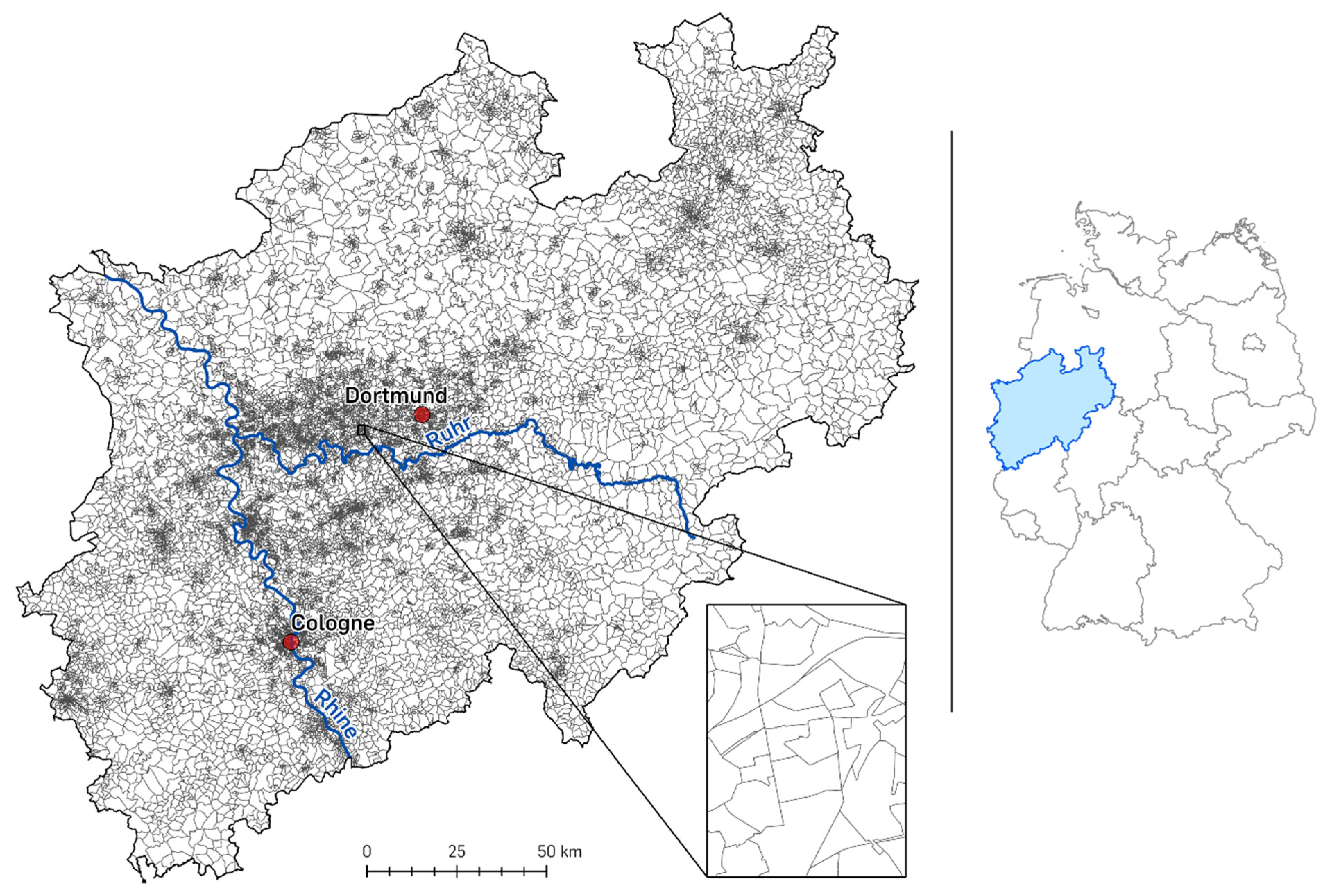
One of the common spatial units for geo-spatial representations of socioeconomic datasets in Germany are postcode polygons. These can be compared to any other kind of gapless spatial unit in terms of global transferability. Those postcode polygons are split up to even more detailed postal units with eight-digit pseudo-postcode polygons (PLZ8) that are provided by the company microm GmbH. Each of the polygons covers about 500 households. Hence, this dataset delivers a uniform basis for comparing different regions while still neglecting the fact that the distribution of people in a given polygon is never homogeneous and, consequently, partly contains areas where no people live. Yet, those homogeneous numbers of inhabitants per unit reliably allow to compare certain attributes in between any selection of polygons ([16], see Figure 1).
In this paper, the general concept of the three-class dasymetric mapping disaggregation will be introduced, illustrated, and applied to income and population data from the city of Dortmund. The resulting disaggregated datasets will be used for spatial comparison of the relationship between the population density and annual income [17] on a city block level. Subsequently, the results will be compared to the initial postal code units through a correlation analysis followed by an individual clustering of both kinds of units for the final identification of respective hot spots of the highest correlation.
Univariate and bivariate choropleth maps are well-suited to give an extensive overview of how people of different economic statuses are distributed in Germany’s most populated state NRW and where certain characteristics and values peak locally. In this case, this comparative visualisation focuses on the two agglomerations of the Rhineland and the Ruhr area with their respective biggest cities of Cologne and Dortmund. They are known to be the densest populated areas in NRW. However, they differ in various social aspects, as, e.g., [18,19,20] have already pointed out. Here, they provide an ideal use case for large-scale disaggregated socioeconomic datasets. A spatial comparison of these two areas reveals patterns that confirm and underline differences, allowing a better understanding of the causes for regional disparities.
The comprehensive disaggregation approach tested for the city of Dortmund refines the PLZ8-wide information to much smaller spatial units representing only residential housing blocks or even single houses and leaving out all unpopulated parts between them. Consequently, disaggregated values can provide the possibility to not only rate the gapless and coarse polygons coming from, e.g., postal codes or administrative units. With them, one can also obtain a visual impression of how the bivariate choropleth map results of the precedent analysis refer to the real living location of the population [21].

2. Materials and Methods

2.1. PLZ8 Polygons

Countries are subdivided into smaller administrative units (states, districts, municipalities, etc.) as well as postal tracts on different levels of spatial detail. The postal code 8 level (PLZ8) is an artificial spatial unit developed for German conditions by microm GmbH. It subdivides the regular German five-digit postal code polygons into smaller areas representing an average of 500 inhabitants per polygon. Advantageously, the PLZ8 data product matches with existing administrative spatial units. Hence, its comparability is directly dependent on the spatial scale of the scientific approach (see Figure 1). In urban areas, one identifies smaller PLZ8 polygons, whereas in rural areas, the extent of PLZ8 polygons is much larger. This means, in effect, that values between two different polygons—e.g., one in an urban and one in a rather rural area—can be reasonably compared with one another while the extent of the respective polygons may differ widely.

2.2. Population Density

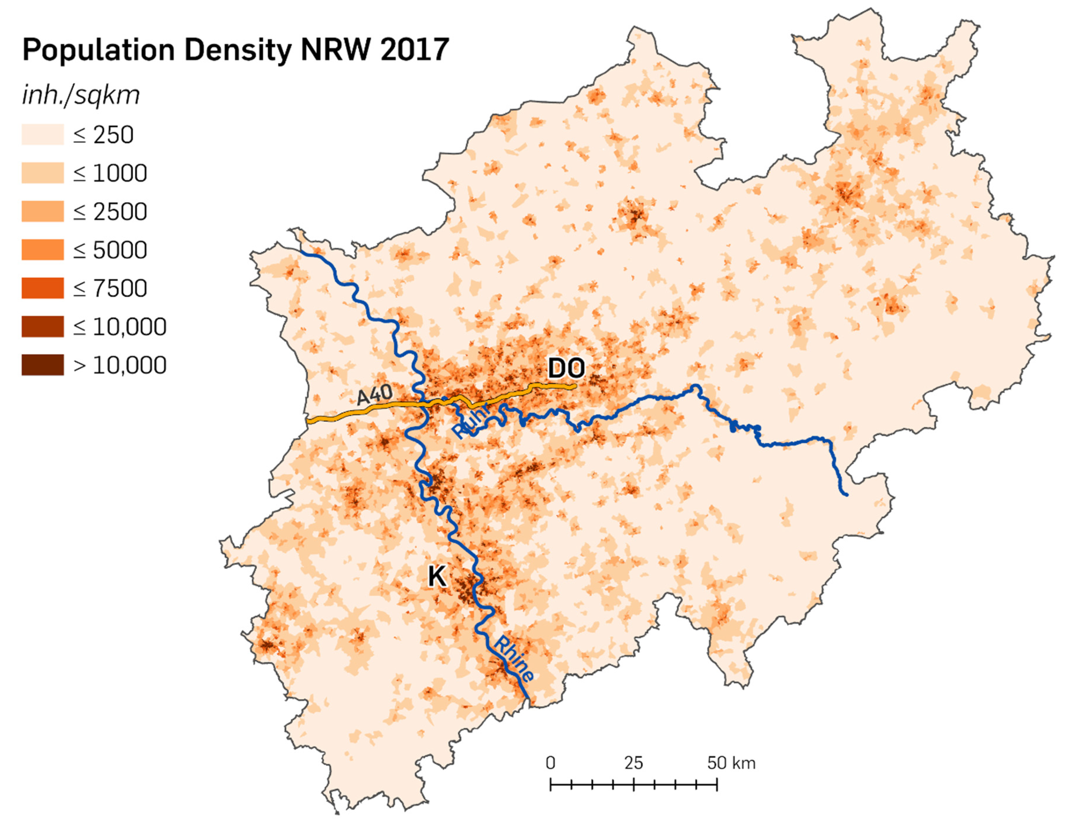
To visualise the population density for each PLZ8 polygon in NRW, the absolute numbers of inhabitants (inh.) must be linked to the extent of the respective polygons in order to be able to calculate the number of inhabitants per square kilometre (sqkm) for each area. After that, the values can be categorised into classes for better comparability [24] and then be visualised in a map (see Figure 2).
The map reveals the more densely populated areas in NRW in darker colours, as there is the Rhine–Ruhr area in its centre with Dortmund (DO) north of the river Ruhr, continuing south across the river Rhine with the city of Cologne (K). All other cities are not named on the map.

2.3. Average Annual Income per Inhabitant

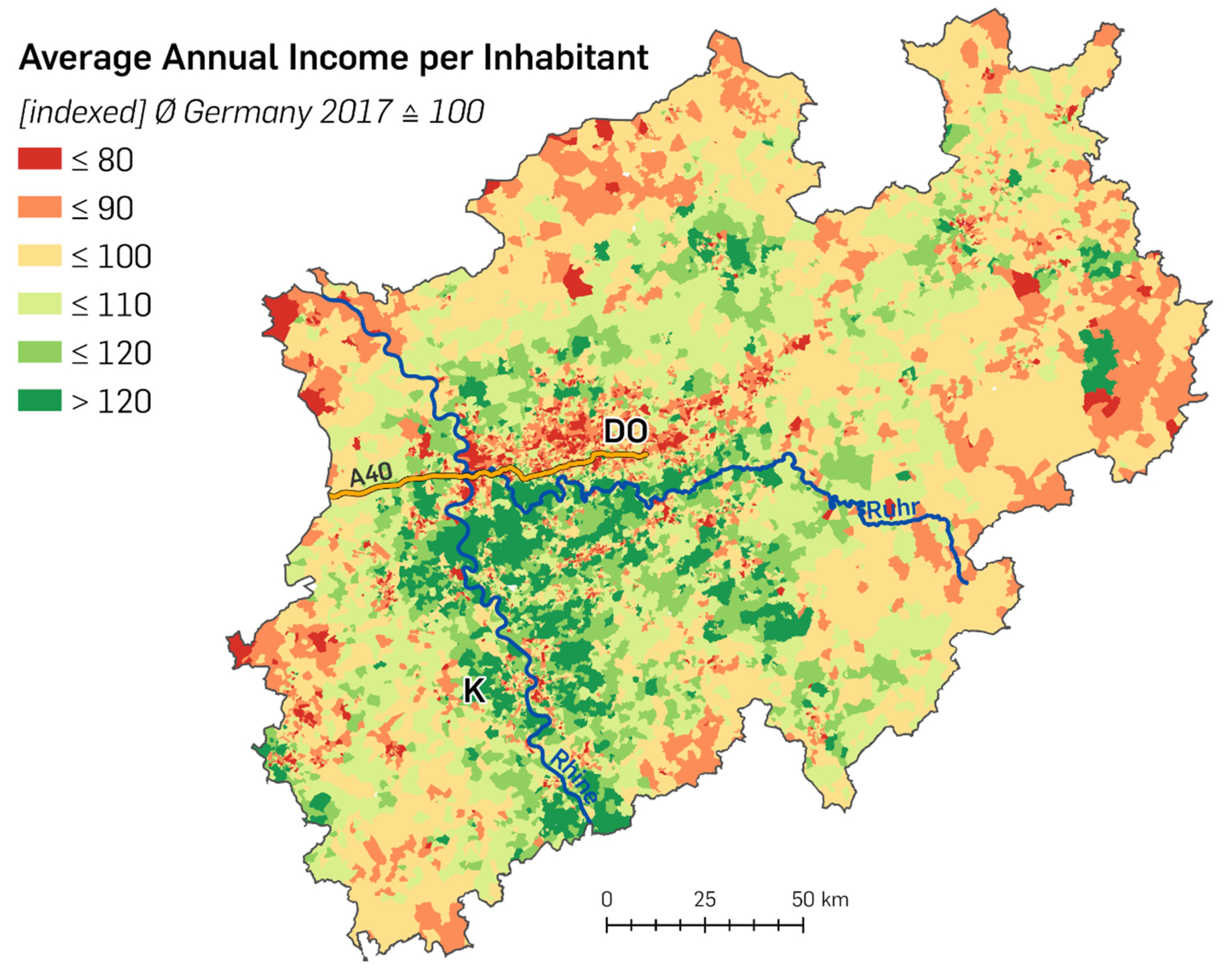
The average annual income per inhabitant can be represented by the monetary sum of money per inhabitant or—better suited for comparisons—by an index that transforms the mean annual income of all inhabitants within a certain year to the value of 100. Income values higher or lower than the average are represented by values above or below 100, respectively. The microm datasets offer a variable called purchasing power index (PPI). It reflects the mean net inhabitant income [27] during the period of 1 year within a spatial unit and can be used as a proxy to assess income factors such as salary, capital assets, lettings, etc., including tax deductions. Periodic expenses such as rent, electricity, and insurances are not taken into account [28]. For Germany, the average income in 2017 is 21,220 EUR per inhabitant and is represented by a PPI value of 100 for that year [17].
The choropleth map of the PPI—more suitable called average annual income per inhabitant hereinafter—for NRW in Figure 3 was created in the same way based upon the same spatial units (PLZ8) as the population density map in Figure 2. It varies the colour scheme for the different classes to point out regions characterised by average, lower, or higher income values (see Figure 3).
As stated before, each PLZ8 unit does not necessarily reflect the real situation of the distribution of inhabitants, as there are areas within each polygon that are not occupied by residents. In order to move these values into those particular sub-polygons, representing the actual location of residential blocks, in the following chapters, a disaggregation approach will be applied. The aim is to confirm the hypothesis that large-scale units, selected as residential areas by their type of usage, provide a significantly better basis for a valuation concerning scientific problems with a spatial socioeconomic background.

2.4. Disaggregation Approach

The disaggregation of spatial data is a problem that widely occurs in science and in planning practice. The primary goal is to distribute values from higher-level, larger spatial units to the smaller spatial units within. Thus, using a suitable procedure that achieves a realistic reassignment of attribute values describing the actual state of the respective smaller spatial units. The method used to assign the aggregated characteristics from the large spatial units—source polygons—to the smaller spatial units—target polygons (see Figure 4)—is crucial for the reliability of a spatial disaggregation on the one hand. On the other hand, the consistency of the input data required for the respective methods has an even higher influence on the quality of the results [29].
Numerous studies conduct a disaggregation using the areal interpolation approach, which is one of the simplest disaggregation techniques (e.g., [31,32]). In contrast, this study applies the three-class dasymetric mapping method as a methodology for further studies in other countries that might be based on it. This approach was evaluated as the best and most accurate one in various studies [29,33,34,35,36]. It is applied by incorporating certain additional datasets that shape and qualify the target areas according to their usage: the outline of city blocks, their individual type of residential use (such as residential, mixed use, etc.), and the coverage of the area by buildings within the respective spatial unit. With this information added to the target polygons, for each of them, a weighting factor can be determined that defines the proportional assignment of inhabitants from the superior PLZ8 polygon. It is also dependent on the extent of each new and smaller spatial unit. The lack of ubiquitous, available, large-scale datasets holding the necessary information for the determination of the weighting factors might be one of the main reasons why so many past studies rather use the much simpler areal interpolation.
Since the availability of datasets required for this approach has strongly improved in a lot of countries over the past years [37,38], with this study, a methodology is developed utilising certain types of broadly available datasets necessary for a dasymetric mapping in three classes. It also aims to advertise this approach for a broader application in socio-geomatic research.
However, still, the general availability of additional datasets depends strongly on the location of the study area and the respective national or regional players that collect and provide the corresponding data. Not only the acquisition of the data itself is important, but also the underlying structure of it. In some three-class approaches, no distinction is made between populated and non-populated target areas. Instead, regardless of whether it is used for, e.g., agricultural, industrial, or residential purposes—a corresponding value of socio-demographic and -economic properties is assigned to each area. While the decision about the weighting factors based on use classes is always subject-driven, it gives degrees of freedom for applying the principle and deriving a suitable allocation factor. Thus creating a need for testing and refinement [35].
As it is known that people use to live in buildings, one could come to more prominent results by focusing the socioeconomic data to build up populated structures. To achieve this, the disaggregation approach is based on remotes-ensing imagery and additional datasets from regional authorities.

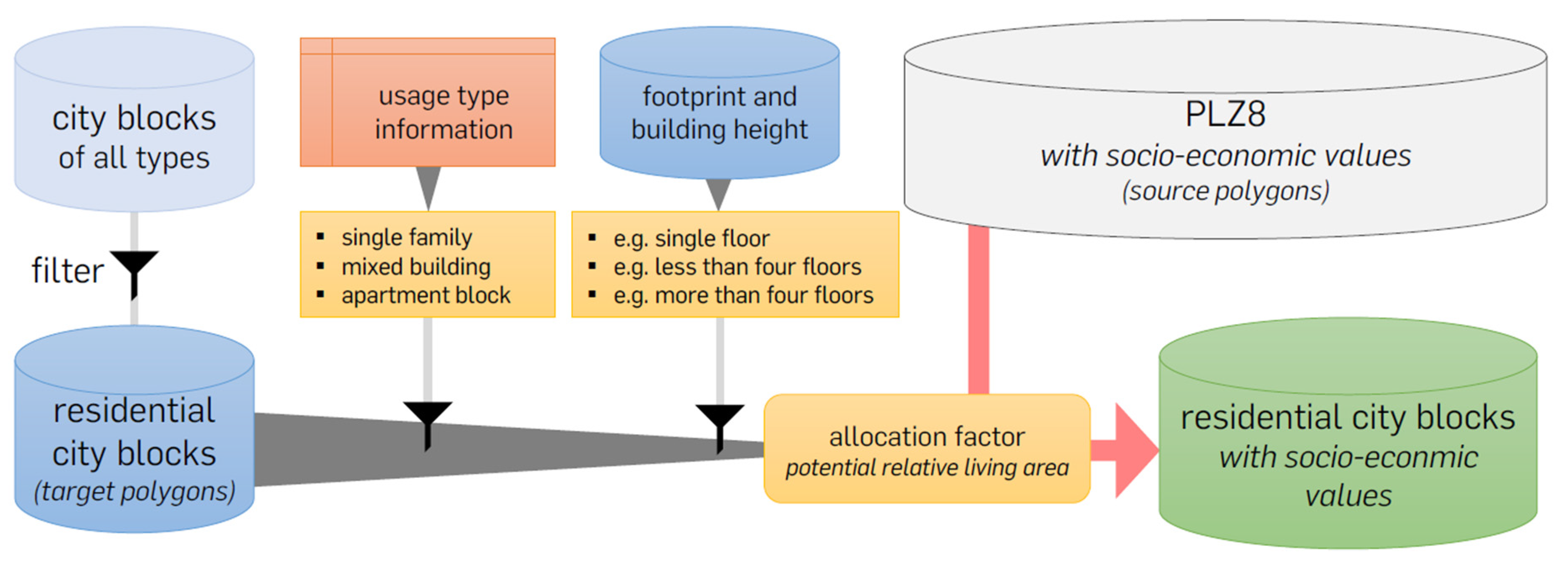
2.5. Disaggregation of Population Density and Annual Individual Income

The disaggregation of the socio-demographic values from the source polygons into the target polygons is conducted in four major steps (see Figure 5): first, the additional datasets that constitute the target polygons in an extended dataset are selected, restructured, and adjusted to obtain a structure that matches the one of the source dataset. In this case, the source polygons are derived from the microm PLZ8 units. The target polygons representing city blocks are taken from the Urban Atlas 2012 dataset provided by the Copernicus program [39]. The official digital landscape model that supplies the building geometries for this case study can be retrieved from Geobasis.NRW [40].
The temporal gap between the datasets is disregarded in this context, since the Urban Atlas and the digital landscape model, besides the target-geometries, only contribute information for the classification of residential use types. A divergent acquisition time of only a few years for these datasets is not expected to cause significant inconsistencies.
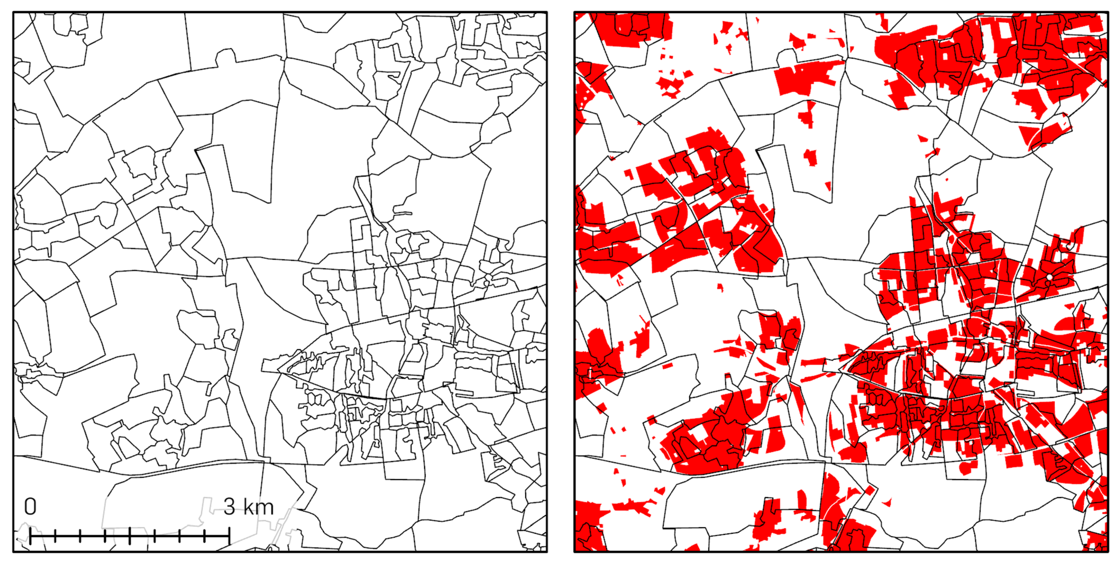
In the second step, representing the second class of the three-class dasymetric mapping process, the extended datasets are filtered according to the requirements for the disaggregation, leaving only the target polygons that are appropriate for the current analysis. In this case study, the residential urban areas providing space for living are of major interest. This leads to preselection of only houses and city blocks whose purpose is habitation as rural, industrial, and commercial sites usually do not provide a place for living. There are several buildings that can be identified as mixed usage, e.g., shops on ground level and several flats on the floors above. This leads to step three, and the third and last class of the disaggregation is where the polygons of the preselected residential areas are classified according to their respective kind of apartment structure and their number of floors [41]. The structure varies from one- or two-floor single homes for single families over mixed buildings with few shops and more apartments to large apartment blocks such as multi-family houses or dormitories for students, pupils, or seniors. Each usage type represents a different amount of people per area unit defining the density of inhabitants in the respective building blocks. This makes it inevitable to distinguish between all these classes, ensuring the values from the source polygons are transferred to the target polygons most appropriately. For this, an allocation factor is determined based on the developed classification of usage types, again based on the additional datasets. This is a crucial step, since the potential relative living area of all subdivided polygons is the only value where all polygons differ from each other.
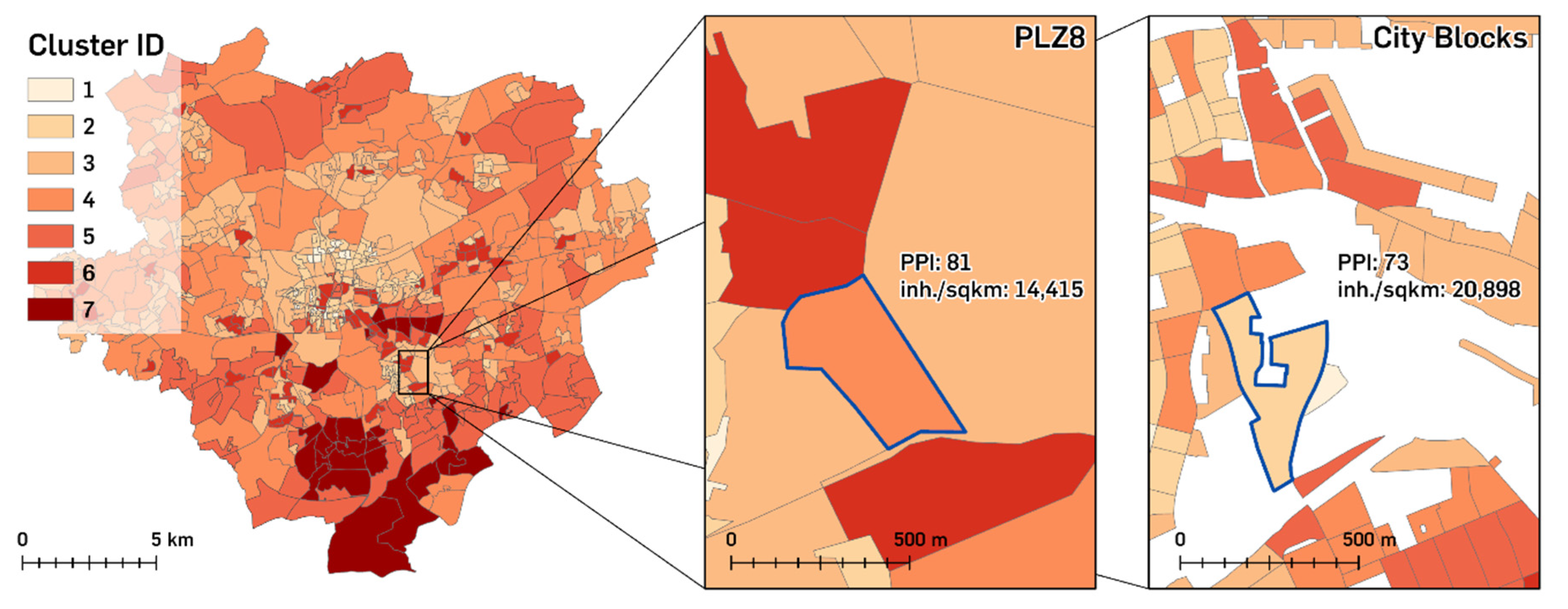
After the preselection and classification of the target polygons, all source polygons are intersected with these prepared target polygons. This step is followed by assigning the weighted source values to the target polygons according to the two steps before. As the PLZ8 and the building block polygons do not match exactly, a lot of target polygons are subdivided into smaller pieces that were assigned with values from different source polygons. These values are assigned to the target polygons depending on their respective potential living area compared to the overall living area in the respective source zones.
Using the specific ID of each single target polygon, these broken parts can be dissolved into a final, coherent city block while aggregating up all property values of the respective subparts. This results in a new patchy dataset covering only those areas where actually people are living.

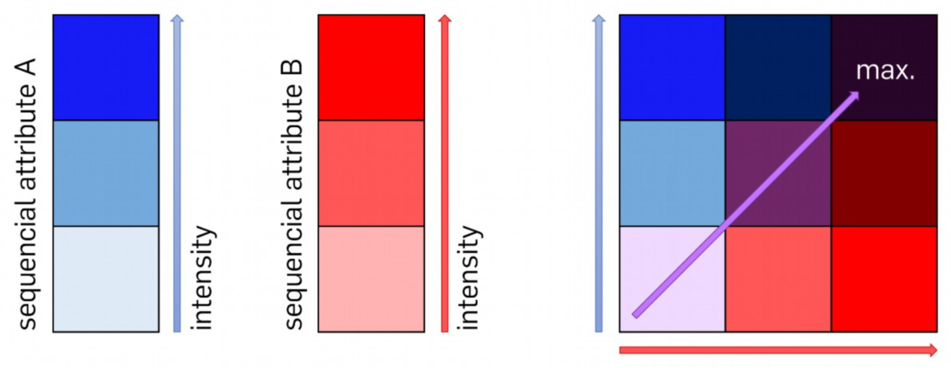
2.6. Concept of Bivariate Choropleth Maps

To illustrate the relationship between two quantitative parameters of polygons in a map, a combined matrix legend can be applied. This supports the recognition of patterns created by the combination of the characteristics of the two variables [42,43]. It is built by combining two different colour scales, each representing one variable by graded brightness. The saturation of the colour assigned to each variable increases with higher values and iss divided into three classes. For easy identification of the displayed correlation, by assigning the resulting colours in the polygons to the combined classes of both variables, a matrix legend with all nine possible colour combinations is used. Therefore, the classes of both characteristics are grouped by a specific selection. This results in an individual associative colour for each possible combination of the two values (see Figure 6). Further applications for bivariate choropleth maps are provided by, e.g., [21,44].

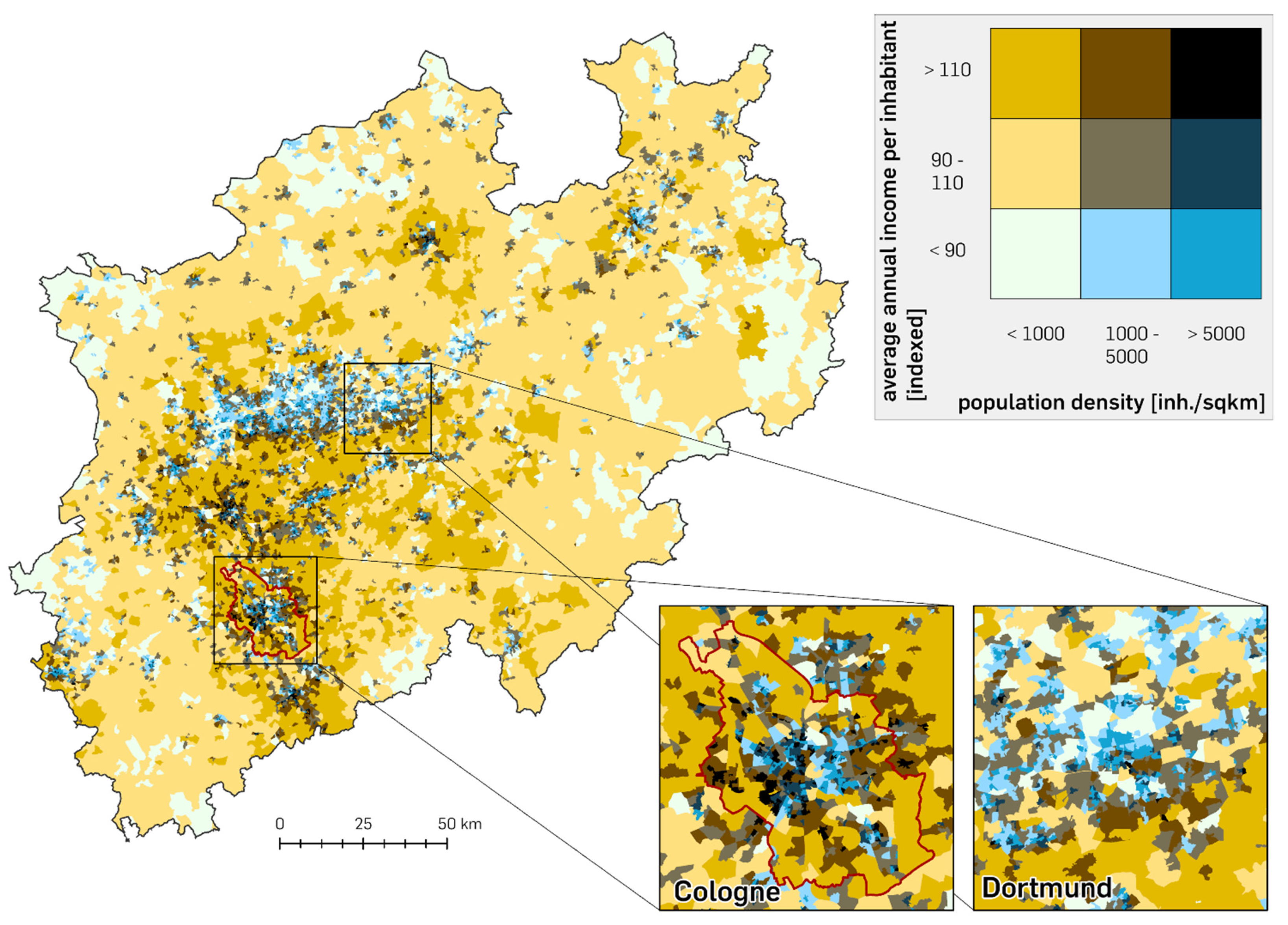
2.7. Population Density vs. Annual Individual Income in Bivariate Choropleth Maps

The univariate choropleth maps shown in Figure 2 and Figure 3 can now be transformed into one bivariate choropleth map. For this reasonable class, breaks for each attribute need to be set, and a colour scheme must be selected that emphasises the essence of this analysis.
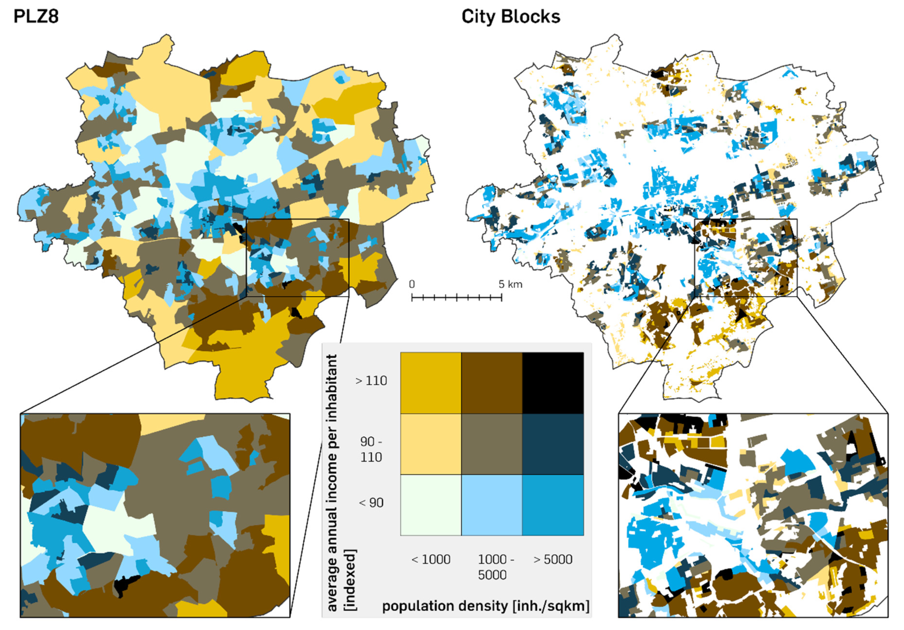
The resulting Figure 7 gives a decent insight into the spatial pattern of the two variables used. It shows less saturation in the combination of the two different colours where values tend to be lower, and vice versa.

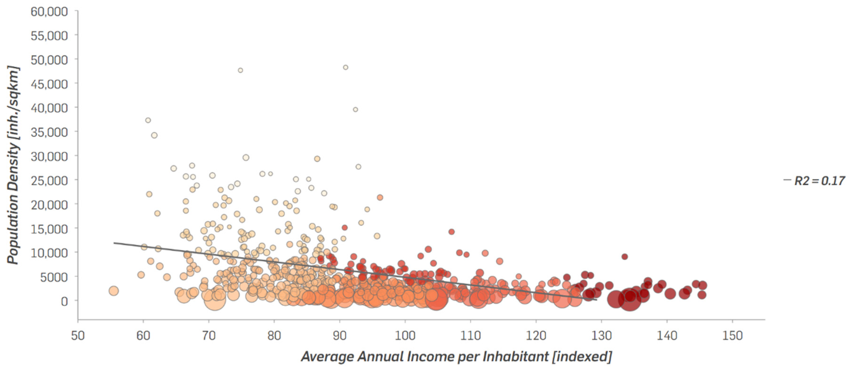
2.8. Correlation and Multivariate Cluster Analysis

The correlation analysis of the two attributes, population density and average annual income per inhabitant, on the PLZ8 level reveals, respectively, a low R2 value with an excessive scattering (see Figure 8).
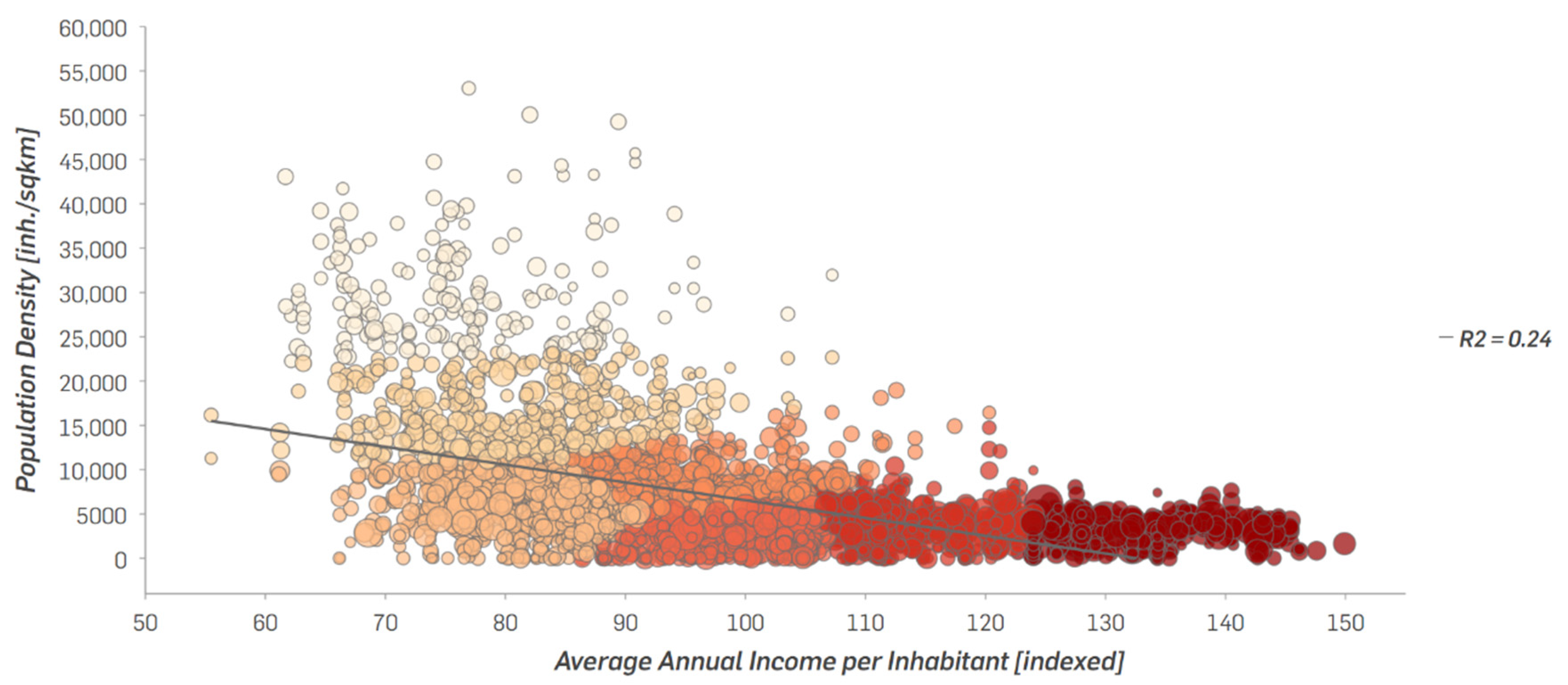
Calculating the same correlation for the disaggregated city block polygons, the R2 value becomes significantly higher while the scattering is reduced (see Figure 9).
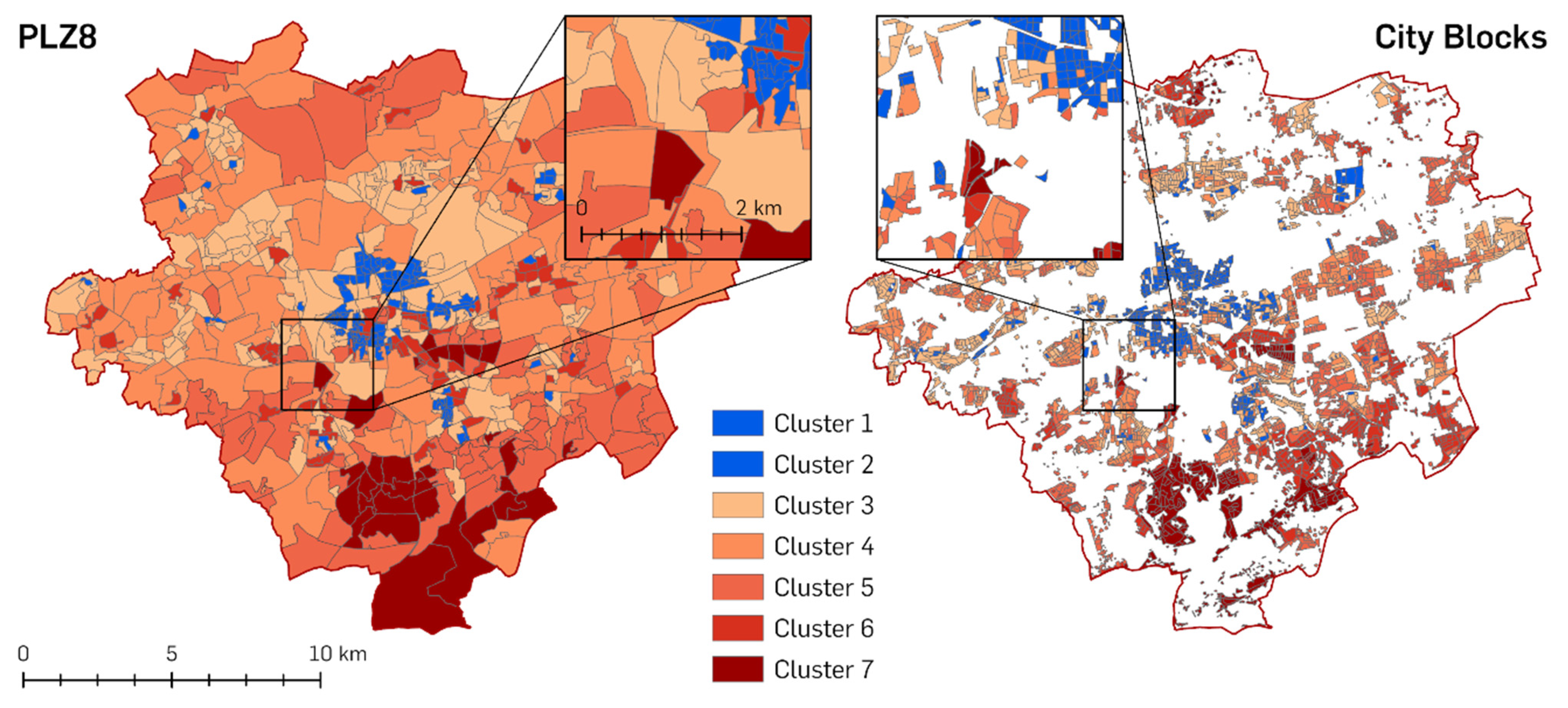
The two regressions already show that the disaggregation has led to an improvement in the correlation of the two values. In the following step, a multivariate cluster analysis is conducted with the two attributes for both spatial units in order to generate new classes, compare the results, and provide a better mean to see if the results can reveal new patterns and insights into large-scale city areas, using the disaggregated city blocks as the smaller spatial unit. The multivariate cluster analysis used in this study is based on the K means algorithm, which aims to partition features based on seeds that grow into clusters, minimising the differences among the features within each cluster [45,46]. This is the basis for the map shown in Figure 10 displaying the clustered values spatially that are shown statistically in the scatterplots of Figure 8 and Figure 9.

3. Results

3.1. Disaggregation

The result of the disaggregation case study for the city of Dortmund leads to two comparable maps, as shown in Figure 10. On the left side, the city of Dortmund is composed of PLZ8 polygons, while the map on the right side shows only residential patches. Looking at the PLZ8 map, it becomes apparent that the level of detail and the variation of colours for the same expanse in the city centre is much higher compared to the outskirts. This can be explained by the requirement of about 500 households per polygon for the PLZ8 data. In less populated areas, these turn out to be larger than those in the city centre, where higher densities of people are present. The polygons in the right map represent only those city blocks where people actually live. All other city blocks (such as open space, industry, business, sports, public services, etc.) were excluded from the disaggregation (white areas in the map). Consequently, the size of polygons representing residential areas is much smaller than the extent of area-wide tracts.
Another improvement is the accuracy of values in certain areas that were transferred from non-fitting geometries to reasonable city blocks (see Figure 11). The Clarenberg in Dortmund’s suburb Hörde is a multi-building residential tower block complex that is home to approximately 3000 people in around 1000 flats. A lot of them are unemployed, there is a relatively high rate of child poverty, and a lot of the inhabitants are receiving unemployment benefits [47]. Thus for the Clarenberg, the average annual income per inhabitant is comparatively low, and the population density—due to the structure of the building complex—is comparatively high. This results in the logical conclusion that it should be represented by one of the lowest clusters that have been calculated by multivariate clustering. Figure 11 shows that this is not the case when looking at the results of the PLZ8 clustering. This is probably caused by the fact that the outlines of the main polygon, which has the biggest overlaying area with the Clarenberg, are not accurately shaped similarly to the complex itself. Hence, the PLZ8 polygon overlays with other surrounding polygons that are not linked with the Clarenberg and represent a respective higher income and a lower population density and are consequently assigned to cluster 4.
The disaggregation outcome shines in a different light—the boundary of the complex is accurately represented by the outline of the polygon, assigned with values that incorporate the structure of the people and the building complex itself. This results in an assignment to the second-lowest cluster by the clustering algorithm applying the disaggregated values stored with city block-polygons. Additionally, the whole level of detail has consequently increased, which leads to a whole new pattern and the possibility of a much finer distinction between the different clusters (see Figure 10). It allows comparing socioeconomic parameters related to single building blocks of homogenous use classes instead of area-wide units with obscurely varying population densities (see Figure 12).
Summed up, the result of the disaggregation is a new sophisticated dataset that contains only building blocks reasonably attributed with values derived from the PLZ8 data and consequently allows evaluating the area in a much more detailed way than the area-wide PLZ8 polygons would allow [5,48]. Now it is possible to distinguish between small housing blocks of fewer or more inhabitants and to directly utilise the focused socioeconomic information about people living there. The value of disaggregated data is to be illustrated in an example by placing focus on a magnified, more detailed sub-area of Dortmund. At this scale, the original PLZ8 data can be ideally compared to the respective disaggregated values. In addition, it can be observed to what extent this higher level of detail can lead to better perceptions.

3.2. Univariate Choropleth Maps

The univariate choropleth maps in Figure 2 and Figure 3 reveal different regional patterns. In the population density map in Figure 2, the densely populated areas appear in darker colours, representing a high number of inhabitants per square kilometre. Namely, there is the dominant Rhine–Ruhr area along the two rivers in the centre of NRW, including the area called ‘Bergisches Land’ south of the Ruhr and several surrounding highly populated areas such as the city of Aachen close to the western border as well as Bielefeld and Münster in the northern part of the state. The space in between these highly populated areas is almost uniformly characterised by rural regions and is not as diverse in terms of population density as it appears in the denser populated urban areas. This results from the fact that population density is highly correlated with specific land use [49] as fields, forests, and huge industrial sites (e.g., open-pit mines) are clearly not as suitable for living as residential areas close to urban agglomerates.
The map in Figure 3 also shows a notable pattern, except that this cannot simply be explained by land use and thus by the presence or absence of housing. Indeed, the reddish-coloured polygons indicate a lower average annual income and appear rather accumulated in more urban areas. There are also urban areas as well as rural areas where this assumption does not fit.

3.3. Bivariate Choropleth Maps

The bivariate choropleth map in Figure 7 shows the combined distribution of the population density and the individual annual income for the year 2017 based on PLZ8 polygons. It is clearly recognisable that the most populated urban areas are dominated by the largest diversity while the rural areas are coloured quite homogenously with less population density and a mediocre annual income. The Ruhr area is dominated by blue polygons, representing the lowest class of average annual income, no matter how densely populated they are. Consequently, this indicates the presence of people who have a low annual income but still live in the rather highly populated inner parts of the cities. This impression is interrupted by only a few areas that are represented in brownish colours. These yellow-brown colours represent the intermediate and utmost class of the individual annual income and are located mostly in the southern parts of the Ruhr area at the northern riverside of the Ruhr. This impression matches with the already attested assumption that the motorway A40 running from west to east across the Ruhr area is some sort of social equator, dividing the Ruhr area into two different parts—well-heeled inhabitants in the southern part and inhabitants with less money in the northern part [50,51].
Comparing the Ruhr area with the Rhineland in Figure 7, one can ascertain that almost no black dyed polygons can be found in the Ruhr area. It appears mostly in lighter colours, indicating the lowest class of the average annual income through all three classes of the population density. Cities such as Dusseldorf, Cologne, or Bonn shine in a different light, since there are a lot of areas that have the highest population density and are indwelled by people who have a relatively high average annual income. The rural areas appear in mostly brownish colours resulting from the already mentioned low rate of population density. They are only interrupted by few smaller areas. These appear either in darker yellow, indicating higher annual income if they are closer to urban agglomerations. Otherwise, they appear in light green in regions far off the respective centres of cities.
The detailed regional perceptions coincide with the statistical results from other studies that analysed the relationship between the Rhineland and the Ruhr area [18,19,20,52]. On the one hand, this corroborates the hypothesis that the social composition of the two agglomerations varies significantly. On the other hand, it provides a possibility to locate these areas in a new level of detail. However, the bivariate choropleth map in Figure 7 can reveal a whole new level of detail and give extensive insights into the smaller urban areas. Additionally, and maybe rather especially, the preceding disaggregation and the resulting new bivariate choropleth map for the city of Dortmund in Figure 12 show that the level of spatial information has increased significantly. This offers the possibility to not only evaluate the bigger picture but also to analyse socioeconomic conditions on a city block level.

4. Discussion

The primary methodological goal of this study was to develop a transferable methodology to be able to analyse socio-demographic variables in much more spatial detail to gain more spatially precise information on the living circumstances of residential areas, embedded in the context of political decision making, geo-marketing, and for further socioeconomic research and urban planning. The results facilitate a distinctly new perspective on certain urban areas, where large-scale city block polygons have replaced the area covering PLZ8 polygons, assigned with respective matching and adjusted values. These allow a much more detailed assessment of fine-grained regional questions.
This becomes obvious by combining the two different socio-demographic attributes of population density and average annual income per inhabitant. This is useful to not only analyse how these two variables may affect each other in terms of numbers but also to dissipate them into appropriate spatial units. Their spatial visualisation can reveal certain segmentations that are perfect for preliminary analyses of the underlying data. By completing this, the results in Figure 7 reveal a distinct pattern that allows for the evaluation and comparison of certain regions about their characteristics in both variables. The K means algorithm and the resulting multivariate statistical and spatial clusters for both spatial levels of detail evidently illustrate the added value of more precise new spatial units that can lead to a better understanding of where to find socially disadvantaged people on the one hand and how to improve economic approaches that incorporate the social status of people on the other hand. They provide an enhanced reference for further studies that deal with a smaller area of investigation and thus require smaller units to evaluate not broadly but in great detail.
Looking at the two regions of the Rhineland and the Ruhr area, it is noticeable that even though both regions stand out in NRW in terms of population density, the Rhineland is obviously inhabited by more people that have an average income or above while the inhabitants of the Ruhr area seem to be below the German average of the respective year (2017). A reason for this could be the diverging demographic structures of the two regions. The Ruhr area has always been a melting pot for miners and factory employees due to the history of the region with a high density of coal and steel factories. Once the industrial sector was obliterated by the structural transformation of the Ruhr area due to the end of the mining era, a lot of people—especially foreign guest workers—were forced to look for new professions while the area was still looking for its future purpose [53]. Apart from that, the Ruhr area had and still has a reputation that suggests a dirty image caused by industrial smoke, coal mining, air pollution, and missing recreational sites such as green areas and forests. This led to the fact that the Rhineland seemed to be more attractive not only for citizens but also for industry and commerce [20] while the Ruhr area was still in the process of handling the downfall of the industrial era and hence is still looking for new perspectives to provide jobs for the many inhabitants.
Due to the successful disaggregation, now inhabitants can be evaluated according to their density and their average annual income—not only for large PLZ8 polygons but for detailed polygons that represent residential city blocks.
Many disaggregation techniques have already been tested, evaluated, and established in various studies (see Section 2.3). However, the one that [21] was adopted and improved for his case study of NRW can easily be transferred to almost every spatial unit in other countries with a comparable data basis without further adaptation. This indicates that socio-geomatic approaches are of great value to combine fine spatial structures with socio-demographic and -economic data to enhance their spatial resolution in order to more accurately analyse their spatial patterns.

5. Conclusions

This paper exemplarily investigates the spatial relationship between population density and annual income to identify hotspots of imbalance by visualising them in bivariate choropleth maps. This approach is carried forward and followed by applying a spatial disaggregation technique to then perform a statistical multivariate cluster analysis on both spatial resolutions for the two attributes into a certain hierarchy for the study area of Dortmund (see Figure 8, Figure 9 and Figure 10).
The comparison of both the clusters and bivariate choropleth maps of the starting and the resulting scales after the disaggregation revealed several improvements. It was demonstrated that the scattering of the cluster combinations has been substantially decreased while the coefficient of determination of the two attributes has been increased, and hence, the usability of socio-demographic values stored in postal code features could be significantly improved.
The empirical acquisition and commercial or scientific distribution of statistical values for the huge variety of different socio-demographic variables is often carried out in coarse and gapless spatial datasets (e.g., regular rasters or postcode polygons). These datasets can help to characterise regions based on their structure and distribution, but their mediocre level of detail and the fact that they do not distinguish between inhabited and uninhabited areas reveal a great potential for improvement concerning the spatial resolution and suitability of the variable containing features. This especially takes effect when dealing with sociological research questions that are analysed spatially, as the results of a sophisticated disaggregation can raise possible interpretations to the next level.

Author Contributions

Conceptualisation, Carsten Juergens, Nicolai Moos, and Andreas P. Redecker; Methodology, Nicolai Moos and Andreas P. Redecker; Spatial Analysis, Nicolai Moos and Andreas P. Redecker; Writing—Original Draft Preparation, Nicolai Moos, Carsten Juergens, and Andreas P. Redecker; Writing—Review and Editing, Nicolai Moos, Carsten Juergens, and Andreas P. Redecker; Visualisation, Nicolai Moos, Carsten Juergens, and Andreas P. Redecker; Supervision, Carsten Juergens. All authors have read and agreed to the published version of the manuscript.

Funding

The research was supported by project no. 2019-1-CZ01-KA203-061374 Spatial and economic science in higher education—addressing the playful potential of simulation games (Spationomy 2.0) funded by the European Union within the Erasmus+ program.

Conflicts of Interest

The authors declare no conflict of interest.

References

  1. Hoffmeyer-Zlotnik, J.H.; Warner, U. Soziodemographische Standards//Nationale soziodemographische Standards und international harmonisierte soziodemographische Hintergrundvariablen. In Handbuch Methoden der empirischen Sozialforschung; Baur, N., Blasius, J., Hoffmeyer-Zlotnik, J.H., Warner, U., Eds.; Springer VS: Wiesbaden, Germany, 2014; pp. 733–743. [Google Scholar]
  2. Küppers, R. Verfahren der Generierung mikrogeographischer Datenangebote zu Bevölkerung, Haushalten, Wohnungen, Gebäuden, Quartieren und Arbeitsplätzen. In Flächenutzungsmonitoring IV: Genauere Daten–Informierte Akteure–Praktisches Handeln; Meinel, G., Schuhmacher, U., Behnisch, M., Eds.; Rhombos: Berlin, Germany, 2012; pp. 175–182. [Google Scholar]
  3. Monteiro, J.; Martins, B.; Pires, J.M. A hybrid approach for the spatial disaggregation of socio-economic indicators. Int. J. Data Sci. Anal. 2017, 5, 189–211. [Google Scholar] [CrossRef]
  4. Yao, J.; Mitran, T.; Kong, X.; Lal, R.; Chu, Q.; Shaukat, M. Landuse and land cover identification and disaggregating socio-economic data with convolutional neural network. Geocarto Int. 2019, 35, 1109–1123. [Google Scholar] [CrossRef]
  5. Stevens, F.R.; Gaughan, A.E.; Linard, C.; Tatem, A.J. Disaggregating census data for population mapping using random forests with remotely-sensed and ancillary data. PLoS ONE 2015, 10, e0107042. [Google Scholar] [CrossRef] [Green Version]
  6. Flacke, J.; Köckler, H. Spatial urban health equity indicators—A framework-based approach supporting spatial decision making. In Proceedings of the Sustainable Development and Planning VII, Istanbul, Turkey, 19–21 May 2015; pp. 365–376. [Google Scholar]
  7. Maschewsky, W. Umweltgerechtigkeit: Gesundheitsrelevanz und Empirische Erfassung; WZB Berlin Social Science Center: Berlin, Germany, 2004; SP I 2004-301. [Google Scholar]
  8. Maier, W.; Mielck, A. “Environmental justice” (Umweltgerechtigkeit). Prävention Gesundh. 2010, 5, 115–128. [Google Scholar] [CrossRef]
  9. Luc Anselin. Spatial Data Analysis with GIS: An Introduction to Application in the Social Sciences; University of California: Santa Barbara, CA, USA, 1992. [Google Scholar]
  10. Ballas, D.; Clarke, G.; Franklin, R.S.; Newing, A. GIS and the Social Sciences: Theory and Applications; Routledge: Abingdon, UK; New York, NY, USA, 2017; ISBN 9781317638834. [Google Scholar]
  11. Goodchild, M.F.; Anselin, L.; Appelbaum, R.P.; Harthorn, B.H. Toward Spatially Integrated Social Science. Int. Reg. Sci. Rev. 2000, 23, 139–159. [Google Scholar] [CrossRef]
  12. Baur, N.; Hering, L.; Raschke, A.L.; Thierbach, C. Theory and Methods in Spatial Analysis. Towards Integrating Qualitative, Quantitative and Cartographic Approaches in the Social Sciences and Humanities. Hist. Soc. Res. 2014, 39, 7–50. [Google Scholar] [CrossRef]
  13. McLafferty, S. The Socialization of GIS. Cartogr. Int. J. Geogr. Inf. Geovis. 2004, 39, 51–53. [Google Scholar] [CrossRef] [Green Version]
  14. Spielman, S.E.; Thill, J.-C. Social area analysis, data mining, and GIS. Comput. Environ. Urban Syst. 2008, 32, 110–122. [Google Scholar] [CrossRef]
  15. Flacke, J.; Schüle, S.A.; Köckler, H.; Bolte, G. Mapping Environmental Inequalities Relevant for Health for Informing Urban Planning Interventions—A Case Study in the City of Dortmund, Germany. Int. J. Environ. Res. Public Health 2016, 13, 711. [Google Scholar] [CrossRef] [Green Version]
  16. Microm GmbH. Das Datenhandbuch 2019. Available online: https://www.microm.de/fileadmin/microm_Datenhandbuch_2019.pdf#c915 (accessed on 15 October 2020).
  17. Microm GmbH. Kaufkraft. Available online: http://fdz.rwi-essen.de/files/PDF/microm_Kaufkraft%20-%20Kopie.pdf (accessed on 15 October 2020).
  18. Tenfelde, K.; Ditt, K. (Eds.) Das Ruhrgebiet in Rheinland und Westfalen; Verlag Ferdinand Schöningh: Paderborn, Germany, 2007; ISBN 9783657757480. [Google Scholar]
  19. LZG. NRW. Bevölkerung Mit Migrationsgeschichte 2017. Available online: https://www.lzg.nrw.de/00indi/0data/02/grafik/0200601052017/atlas.html?comparisonSelect=5000&date=2017 (accessed on 20 October 2019).
  20. Ditt, K. Die Entwicklung des Raumbewusstseins in Rheinland und Westfalen, im Ruhrgebiet und in Nordrhein-Westfalen während des 19. und 20. Jahrhunderts: Charakteristika und Konkurrenzen. In Das Ruhrgebiet in Rheinland und Westfalen; Tenfelde, K., Ditt, K., Eds.; Verlag Ferdinand Schöningh: Paderborn, Germany, 2007; pp. 405–473. ISBN 9783657757480. [Google Scholar]
  21. Moos, N. Soziogeomatik: Möglichkeiten und Grenzen der Verwendung von Erdbeobachtungsdaten und Geodaten Zusammen mit Soziodemographischen und Sozioökonomischen Daten. Ph.D. Thesis, Ruhr-University Bochum, Bochum, Germany, 2020. [Google Scholar]
  22. Microm GmbH. PLZ8: NRW Region. Available online: https://www.microm.de/loesungen/geodaten/plz8/ (accessed on 22 November 2020).
  23. BKG. Verwaltungsgebiete 1:250 000 (VG250). Available online: https://gdz.bkg.bund.de/ (accessed on 21 November 2020).
  24. Juergens, C. Digital Data Literacy in an Economic World: Geo-Spatial Data Literacy Aspects. ISPRS Int. J. Geo Inf. 2020, 9, 373. [Google Scholar] [CrossRef]
  25. Microm GmbH. Soziodemografische Variablen NRW 2017. Available online: https://microm.de/loesungen/marktdaten/soziodemografie-und-oekonomie/ (accessed on 16 October 2020).
  26. Openstreetmap Contributors: OpenStreetMap Data Extracts. Available online: https://openstreetmap.org/copyright;opendatacommons.org (accessed on 22 November 2020).
  27. RWI; Microm. Sozioökonomische Daten auf Rasterebene (Welle 6). Kaufkraft; RWI—Leibniz Institute for Economic Research: Essen, Germany, 2018. [Google Scholar]
  28. Goebel, J.; Krause, P. Gestiegene Einkommensungleichheit in Deutschland. Wirtschaftsdienst 2007, 87, 824–832. [Google Scholar] [CrossRef]
  29. Li, T.; Pullar, D.; Corcoran, J.; Stimson, R. A comparison of spatial disaggregation techniques as applied to population estimation for South East Queensland (SEQ), Australia. Appl. GIS 2007, 3, 1–16. [Google Scholar] [CrossRef]
  30. European Commission. Copernicus. Urban Atlas 2012. Available online: https://land.copernicus.eu/local/urban-atlas/urban-atlas-2012 (accessed on 22 November 2020).
  31. Cartone, A.; Panzera, D. Deprivation at local level: Practical problems and policy implications for the province of Milan. Reg. Sci. Policy Pr. 2021, 13, 43–61. [Google Scholar] [CrossRef]
  32. Kounadi, O.; Ristea, A.; Leitner, M.; Langford, C. Population at risk: Using areal interpolation and Twitter messages to create population models for burglaries and robberies. Cartogr. Geogr. Inf. Sci. 2018, 45, 205–220. [Google Scholar] [CrossRef]
  33. Li, T.; Corcoran, J. Testing dasymetric techniques to spatially disaggregate the regional population forecasts for South East Queensland. J. Spat. Sci. 2011, 56, 203–221. [Google Scholar] [CrossRef]
  34. Mennis, J.; Hultgren, T. Intelligent Dasymetric Mapping and Its Application to Areal Interpolation. Cartogr. Geogr. Inf. Sci. 2006, 33, 179–194. [Google Scholar] [CrossRef]
  35. Eicher, C.L.; Brewer, C.A. Dasymetric Mapping and Areal Interpolation: Implementation and Evaluation. Cartogr. Geogr. Inf. Sci. 2001, 28, 125–138. [Google Scholar] [CrossRef]
  36. Sridharan, H.; Qiu, F. A Spatially Disaggregated Areal Interpolation Model Using Light Detection and Ranging-Derived Building Volumes. Geogr. Anal. 2013, 45, 238–258. [Google Scholar] [CrossRef]
  37. Coetzee, S.; Ivánová, I.; Mitasova, H.; Brovelli, M. Open Geospatial Software and Data: A Review of the Current State and A Perspective into the Future. ISPRS Int. J. Geo Inf. 2020, 9, 90. [Google Scholar] [CrossRef] [Green Version]
  38. Malhotra, A.; Bischof, J.; Allan, J.; O’Donnell, J.; Schwengler, T.; Benner, J.; Schweiger, G. A Review on Country Specific Data Availability and Acquisition Techniques for City Quarter Information Modelling for Building Energy Analysis. In BauSIM 2020: 8th Conference of IBPSA Germany and Austria, 23–25 September 2020, Graz University of Technology, Austria: Proceedings; Verlag der Technischen Universität Graz: Graz, Austria, 2020. [Google Scholar]
  39. Batista e Silva, F.; Poelman, H. Mapping Population Density in Functional Urban Areas: A Method to Downscale Population Statistics to Urban Atlas Polygons; EUR, Scientific and Technical Research Series: Luxembourg, 2016. [Google Scholar]
  40. Land NRW. Open Data-Digitale Geobasisdaten NRW. Available online: https://www.bezreg-koeln.nrw.de/brk_internet/geobasis/opendata/index.html (accessed on 30 April 2020).
  41. Töpsch, S. Räumliche Disaggregation von Bevölkerungsdaten: GIS-Gestützte Methode zur Erstellung eines Deutschland-Rasters der Kleinräumigen Bevölkerungsdichte; Paris Lodron-Universität: Salzburg, Austria, 2009. [Google Scholar]
  42. Götze, W.; van den Berg, N. Techniken des Business Mapping; Oldenbourg Wissenschaftsverlag: Berlin, Germany; Boston, MA, USA, 2003; (Reprinted in 2017). [Google Scholar]
  43. Olbrich, G.; Quick, M.; Schweikart, J. Desktop Mapping: Grundlagen und Praxis in Kartographie und GIS, 3rd ed.; Springer: Berlin/Heidelberg, Germany, 2002. [Google Scholar]
  44. Juergens, C.; Meyer-Heß, M.F. Application of NDVI in Environmental Justice, Health and Inequality Studies–Potential and Limitations in Urban Environments; Preprints: Basel, Switzerland, 2020. [Google Scholar]
  45. Jain, A.K. Data clustering: 50 years beyond K-means. Pattern Recognit. Lett. 2010, 31, 651–666. [Google Scholar] [CrossRef]
  46. ESRI. Mapping Cluster Toolset Concepts: How Multivariate Clustering Works. Available online: https://pro.arcgis.com/en/pro-app/latest/tool-reference/spatial-statistics/how-multivariate-clustering-works.htm (accessed on 29 January 2021).
  47. Stadt Dortmund. Bericht zur sozialen Lage in Dortmund 2018; City of Dortmund, Department for Labor, Health and Social Affair: Dortmund, Germany, 2018. [Google Scholar]
  48. Mennis, J.; Hultgren, T. Dasymetric Mapping for Disaggregating Coarse Resolution Population Data. In Proceedings of the 22nd Annual International Cartographic Conference, A Coruña, Spain, 9–16 July 2005; pp. 9–16. [Google Scholar]
  49. Cooke, S.; Behrens, R. Correlation or cause? The limitations of population density as an indicator for public transport viability in the context of a rapidly growing developing city. Transp. Res. Procedia 2017, 25, 3003–3016. [Google Scholar] [CrossRef]
  50. Kersting, V.; Meyer, C.; Strohmeier, P.; Terpoorten, T. Die A 40–der Sozialäquator des Ruhrgebiets. In Atlas der Metropole Ruhr: Vielfalt und Wandel des Ruhrgebiets im Kartenbild; Prossek, A., Schumacher, J., Eds.; Emons: Köln, Germany, 2009. [Google Scholar]
  51. Mühlan-Meyer, T.; Lützenkirchen, F. Visuelle Mehrsprachigkeit in der Metropole Ruhr–eine Projektpräsentation: Aufbau und Funktionen der Bilddatenbank “Metropolenzeichen”. Z. Angew. Linguist. 2017, 66. [Google Scholar] [CrossRef]
  52. Danielzyk, R. Demographischer Wandel in Nordrhein-Westfalen, 2nd ed.; Inst. für Landes-und Stadtentwicklungsforschung: Dortmund, Germany, 2010; ISBN 9783869340418. [Google Scholar]
  53. Weber, W. Strukturwandel im Ruhrgebiet 1820-2000. Westfälische Z. Z. Vaterländische Gesch. Altert. 2003, 153, 71–83. [Google Scholar]
Figure 1. Location of North Rhine-Westphalia in Germany and its PLZ8 polygons based on postal codes and an average of 500 households per polygon (Data source: [22,23]).
Ijgi 10 00432 g001
Figure 2. Population density 2017 of North Rhine-Westphalia based on PLZ8 polygons, K: Cologne, DO: Dortmund (Data source: [23,25,26]).
Ijgi 10 00432 g002
Figure 3. Average annual income per inhabitant (PPI 2017) for the area of North Rhine-Westphalia based on PLZ8 polygons, K: Cologne, DO: Dortmund (Data source: [23,25,26]).
Ijgi 10 00432 g003
Figure 4. PLZ8 source polygons (black lines) and target polygons (red areas) (Data source: [22,30]).
Ijgi 10 00432 g004
Figure 5. Schematic flow chart of the disaggregation process (source: authors).
Ijgi 10 00432 g005
Figure 6. Schematic generation of a sequential matrix legend (Source: authors).
Ijgi 10 00432 g006
Figure 7. Bivariate choropleth map showing the combination of population density and average annual income per inhabitant (Data source: [22,23,25]).
Ijgi 10 00432 g007
Figure 8. Regression analysis for average annual income per inhabitant and population density in PLZ8 polygons, dot size in scatterplot proportional to relative polygon area (Source: authors).
Ijgi 10 00432 g008
Figure 9. Regression analysis for average annual income per inhabitant and population density in city block-polygons, dot size in scatterplot proportional to relative polygon area (Source: authors).
Ijgi 10 00432 g009
Figure 10. Multivariate clusters for the city of Dortmund with PLZ8 and city blocks, the two lowest clusters in blue (Data Sources: [22,23,25]).
Ijgi 10 00432 g010
Figure 11. Clarenberg building complex (blue outline) in Dortmund—comparison of extent, shape, and values before and after disaggregation (Date source: [22,23,25,40]).
Ijgi 10 00432 g011
Figure 12. Disaggregated values from PLZ8 (left) to residential blocks (right) for the city of Dortmund (Data source: [22,23,25,40]).
Ijgi 10 00432 g012
Publisher’s Note: MDPI stays neutral with regard to jurisdictional claims in published maps and institutional affiliations.

