Article

Modelling Place Visit Probability Sequences during Trajectory Data Gaps Based on Movement History

1
State Key Laboratory of Information Engineering in Surveying Mapping and Remote Sensing, Wuhan University, Wuhan 430072, China
2
Department of Geography & Environment, Western University, London, ON N6A 3K7, Canada
3
School of Geography and Information Engineering, China University of Geosciences, Wuhan 430000, China
*
Author to whom correspondence should be addressed.
ISPRS Int. J. Geo-Inf. 2021, 10(7), 456; https://0-doi-org.brum.beds.ac.uk/10.3390/ijgi10070456
Submission received: 2 April 2021 / Revised: 30 June 2021 / Accepted: 1 July 2021 / Published: 2 July 2021

Abstract

:
The acquisition of human trajectories facilitates movement data analytics and location-based services, but gaps in trajectories limit the extent in which many tracking datasets can be utilized. We present a model to estimate place visit probabilities at time points within a gap, based on empirical mobility patterns derived from past trajectories. Different from previous models, our model makes use of prior information from historical data to build a chain of empirically biased random walks. Therefore, it is applicable to gaps of varied lengths and can be fitted to empirical data conveniently. In this model, long gaps are broken into a chain of multiple episodes according to past patterns, while short episodes are estimated with anisotropic location transition probabilities. Experiments show that our model is able to hit almost 60% of the ground truth for short gaps of several minutes and over 40% for longer gaps up to weeks. In comparison, existing models are only able to hit less than 10% and 1% for short and long gaps, respectively. Visit probability distributions estimated by the model are useful for generating paths in data gaps, and have potential for disaggregated movement data analysis in uncertain environments.

1. Introduction

Information, communication, and location-based technology have boosted the collection of human movement data at the individual level [1,2,3,4], supporting applications in intelligent location-based service and mobility pattern modelling [5,6,7,8,9]. These data sample the location of moving objects at a finite set of moments as a series of timestamped locations, i.e., trajectories [10]. However, many factors, including device power outage, careless shutdown, and poor satellite signal can lead to missing data [11,12]. Low user activity level, low location recording frequency, or privacy awareness may further result in sparse data [13,14]. These problems lead to absent location samples at moments or periods, i.e., trajectory data gaps. In this article, we define gaps as time-continuous episodes with no location fixes in a trajectory.
Gaps can result in biases in trajectory-based analyses and reduced quality of personalized location-based services, which has raised attention in cellular network data analytics [15,16,17]. Compared to cellular data collection that requires little effort by the user, it is more difficult to collect complete trajectories by carrying tracking devices or geotagging social media posts. For example, in a GPS travel survey in three Scottish towns, almost one in five participants carrying GPS units did not return useable data [12]. A study on location-based social networks reported that a user published only one to fifteen geotags per month on average [13]. Therefore, gaps in trajectory data remain a problem requiring further attention in computational movement analysis [6,8], and techniques should be developed to work with gaps in real data from individual users [18].
Statistical imputation handles missing observations in numerical or categorical series [19], but ignores sequential relationships in trajectory data. In longitudinal social science studies, missing data have been a concerning issue in the analysis of life courses [20,21], and multiple imputation by chained equations is effective using multinominal logistic regression model of states before and after a gap [22]. Hidden Markov models [7,23] and neural networks [16,24] can reconstruct missing location series as a sequence, but do not account for physical constraints such as maximum speed. Focusing on the physical dimension of movement, space-time prisms delineate boundary of accessible areas between two points within a time budget. Recent work on movement further differentiates locations within prisms from statistical perspective using visit probabilities [25,26,27,28].
In this study, we proposed a probabilistic space-time model based on historical trajectories (PSM-H) to estimate visit probability distributions during gaps. PSM-H is different from its traditional counterparts, because it captures and makes use of empirical patterns in human movement. Specifically, PSM-H allows chaining of multiple movement episodes according to historical data, which keeps estimation informative for long time spans while prisms from traditional time geography become too large in size. Meanwhile, past movement data are also helpful for realistic estimation of probabilities during short gaps with place and route preference taken into account. The representation of movement preference is useful for user profiling and agent-based models. Visit probability estimations help reconstruct individual trajectory in large spatial extents and for long time intervals [29]. The estimated probabilities may also benefit applications like environmental exposure assessment, as it can help quantify risks associated with dynamic geographic contexts [30].

2. Background

The uncertainty of movement during a trajectory gap is similar to what is modeled by space-time prisms in time geography, i.e., potential trips from an origin to a destination (termed as anchors) within a given time constraint [31]. Winter and Yin [32,33] introduced probability to the description of internal prism structure. Song and Miller [34] formulated Directed Random Walk (DRW) and Truncated Brownian Bridge (TBB) as discrete and continuous stochastic models for movement between anchors. DRW and TBB simulate time series of visit probability distributions (aka. probability surfaces) with speed constraints in Euclidean plane. There are also extensions to allow acceleration constraint [35] and movement within networks [36]. However, these studies do not model habits and preferences of movement.
Individual human movement has intrinsic regularities and patterns [37]. These habitual mobility patterns can help reveal how individuals potentially move during gaps. Holistic methods of social sequence analysis focus on optimal matching and alignment algorithms to identify representative subsequences by similarity metrics [38,39]. Transition probability and sequence frequency have been used to measure the representativeness of a sequence [40,41]. In data science, there are various statistics based on sequences of discrete places and to reflect different aspects of individual movement, including place preference, spatial transition, route preference, and temporal relation. Place stay duration distributions describe preferred length of time of staying at a place [42]. The place pair frequency is the frequency of moving from one place to another [43,44,45,46]. The place sequence frequency extends from pairs to sequences, and differentiates the chances that one travels along a route [47,48]. The frequency of presence at places in relative time calculates the frequency of visiting a place at a relative period, e.g., a month of a year, an hour of a day [5,49]. These factors are useful to model movement habits, such as preference and chains of trips during gaps, when populating stochastic models with empirical parameters.

3. Probabilistic Space-Time Model from Historical Trajectories

In this section, we present how PSM-H estimates place visit probabilities during a gap in three steps. The first step extracts statistical distributions as mobility patterns (Section 3.1). Based on empirical distributions, we enumerate possible ways to break a gap into stops and moves in Section 3.2 as the second step, where each way is a chain of timestamped trip episodes (termed as routes and schedules). For each episode of a chain, Section 3.3 elaborates the final step on how to derive detailed probabilities using directed random walk, with empirically biased convolution kernels.

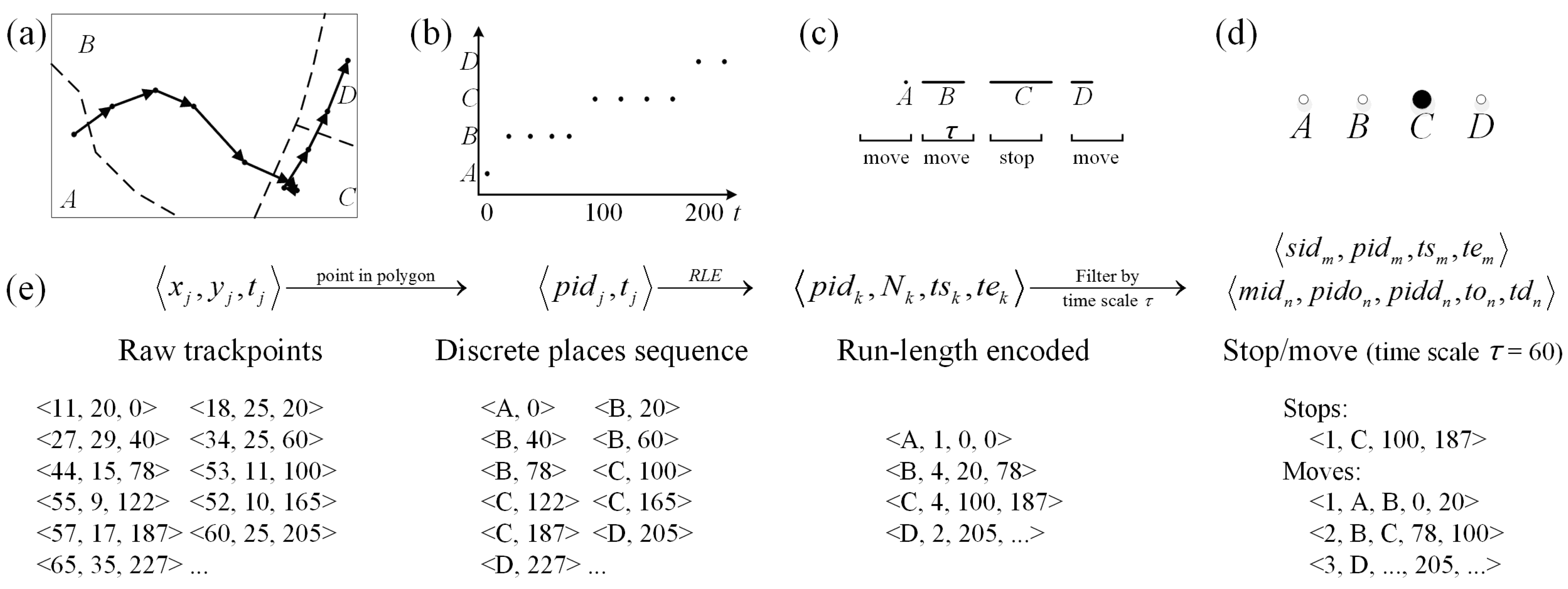
3.1. Mobility Patterns

In PSM-H, mobility patterns are based on preferences of an individual implied by historical trajectories. To reveal patterns, we identify meaningful locations associated with real-world activities as places. For operational simplicity, we use an irregular partition of space to model varied sizes and shapes of places; however, it should be noted that any function mapping geographic coordinates to a place label is compatible. We formalize preference as empirical distributions of certain activities, such as stops and moves. To define activities of stop and move, PSM-H also requires a temporal scale of analysis. A stop is an episode staying at one place for longer than one temporal grain, while a move is the episode between consecutive stops.
Based on places and temporal scale, we define useful forms to represent trajectories for pattern extraction. Symbols used here are listed in Table 1. Given a set of polygons <pidl, polygonl>, location records <xj, yj, tj> in the trajectory data (Figure 1a) can be converted into place sequence <pidj, tj> (Figure 1b) by simple point-in-polygon tests. A sequence can be reduced by merging consecutive appearances of elements, known as the run-length encoding (RLE, [50]). Thus, the RLE representation {<pidk, Nk, tsk, tek>} denotes a trajectory of K episodes with Nk consecutive location fixes at place pidk between timestamps tsk and tek. By comparing the duration of episodes in an RLE representation to a temporal grain (Figure 1c), we derive lists of stops and moves (Figure 1d).
The place sequence {pidj} implies a scale-invariant mobility pattern that reflects the spatiotemporal affinity between a pair of places. We define place adjacency count as the count of occurrences of place a preceding places b in {pidj}.
A C ( a , b ) = | { j | p i d j 1 = a p i d j = b , 2 j J } |
In stop/move representations, there are several scale-dependent mobility patterns. One of them is how long people tend to stay at a particular place. For a list of stops, the distribution of stay duration is defined by Equation (2).
S D ( Δ s ; a ) = | { s i d m | s p i d m = a t e m t s m = Δ s } | | { s i d m | s p i d m = a } | , 1 m M
Another useful pattern is typical time cost for the trip between place pairs. Similarly, for a list of moves, we define the distribution of travel time by Equation (3).
T T ( Δ t ; a , b ) = | { m i d n | p i d o n = a p i d d n = b t d n t o n = Δ t } | | { m i d n | p i d o n = a p i d d n = b } | , 1 n N
To model the route preference between two places, we further exploit the stop list to extract sequence frequency distributions. We search the stop sequence {spidn} for a set of subsequences that serve as possible routes during a gap from o to d by Equation (4). Such subsequences should be no longer than the length of gap, tmax.
R = { s p i d [ m , m ' ] | s p i d m = o s p i d m ' = d t s m ' t e m t max } , 1 m < m ' M
The frequency of a subsequence, r, is defined as its occurrence count normalized by the total counts of subsequences from place o to d (Equation (5)).
S F ( r ) = | { m | r = s p i d [ m , m + | r | ] , 1 m M | r | } , r R | r ' R | { m | r ' = s p i d [ m , m + | r ' | ] , 1 m M | r ' | } |
To account for a detour, which may be caused by barriers or preferences during a directed movement, we also exploit subsequences of RLE. For example, one has to travel west to a gate before leaving for a destination in the east. In this case, it is realistic to consider moving west as toward destination, even if it increases the distance to the destination. Therefore, we define the relative direction of a local movement during a trip based on empirically observed order of places. We find relevant time spans Ssub of all trips from place o to d (Equation (6)), and filter the RLE sequence to get a set S of subsequences representing these trips (Equation (7)). The relative direction of a move from place a to b is determined by the occurrence count of a preceding b during trips in S (Equation (8)). A positive count indicates a local move as moving forward, otherwise not.
S s u b = { ( t o n , t d n ) | p i d o n = o p i d d n = d } , 1 n N
S = { p i d [ k , k ' ] | t s k < t o < t e k , t s k ' < t d < t e k ' } , ( t o , t d ) S s u b
M D ( a , b | o , d ) = | { s | s u = a s u ' = b , 1 u < u ' < | s | , s S } |

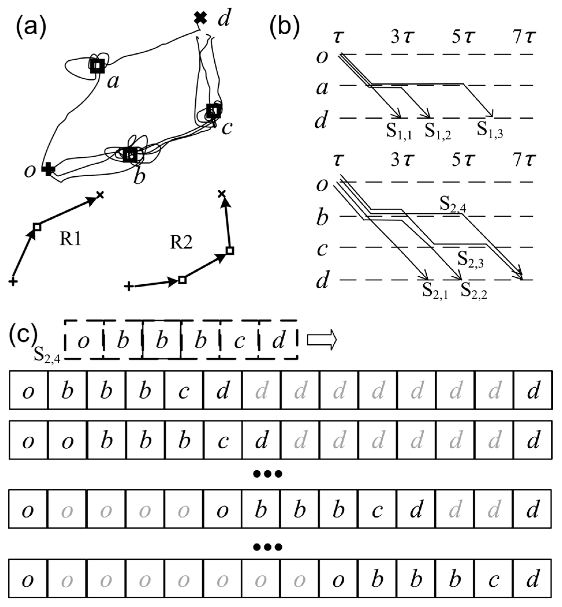
3.2. Routes and Schedules

Movement during a gap may consist of multiple episodes of stops and moves, which is essentially travelling along a chain of waypoints, with the purpose of each move as reaching the next waypoint. In this step, we focus on these waypoints and address how PSM-H divides a gap into multiple sections. Possible place and time of stops will serve as anchors in subsequent model of moves.
In the spatial dimension, we term a possible waypoint sequence during a gap as a route. As defined in Equation (5), sequence frequency SF associates all place sequences with a frequency. Any stop sequence between origin o and destination d serves as a valid route, if the length of the sequence is not greater than the duration of a gap. For example, in Figure 2a, there are two routes R1 and R2 from place o to place d in historical data with different frequencies. In the temporal dimension, specific times for visiting each place in a route is termed as a schedule. It is necessary to define the trips in a chain, because the prisms between the same pair of places are also dependent on time budget. Schedules for two routes are exemplified in Figure 2b. For route R1, schedule S1,1 means the object starts from o at time τ, stays at place a from 2τ to 3τ, and finally arrives at d at 4τ. Each schedule is associated with its historical frequency to model temporal preference. Due to the length difference between the gap and the schedule, there are multiple possible timings for the schedule to happen, i.e., to leave place o (+ marker) later than the head of the gap, and to arrive at place d (×marker) earlier than the tail of the gap (Figure 2c). To assign schedules for generated routes, the possible visiting time series for the waypoints in a route are enumerated by sliding along the gap.
The frequency of each route and schedule is used as a weight when aggregating visit probability distributions of different routes. Corresponding frequencies are counted according to empirical schedules for each route in historical data.

3.3. Visit Probability Estimation

Possible routes and schedules divide the movement during the gap into multiple sections. We then focusing on estimating visit probability series for each section using a recurrent model adapted from a directed random walk (DRW) to incorporate local mobility patterns. The basic idea of a recurrent model is to define an initial state and a recurrence relation between previous and current instants. In this model, a kernel similar to the one used in matrix convolution and image filtering describes the recurrence relation.
To define the kernel, we focus on an arbitrary intermediate move from an intermediate place i at time t to place a in its neighborhood. Such a move during a directed movement must choose one of the following three directions: moving forward, moving backward, and staying. The moving probability for different directions must be weighted properly to reflect the influence of time budget. The choice of staying at place i at time t includes two steps, staying at i for more time and reaching the destination within the remaining time. To leave place i at time t (either moving forward or backward) means to stay at the place until time t and to reach the destination within the remaining time td—t. Hence, the weights for staying and leaving can be formulated as
weight ( stay , i , t | o , t o , d , t d ) = Δ s = t t o t d t o S D ( Δ s ; i ) Δ t = 0 t d t 1 T T ( Δ t ; i , d )
weight ( leave , i , t | o , t o , d , t d ) = Δ s = 0 t t o S D ( Δ s ; i ) Δ t = 0 t d t T T ( Δ t ; i , d )
where o and d are the origin and destination, to and td the corresponding timestamp. SDs;i) denotes the distribution of stay duration Δs at place i. TTt;i,d) denotes the distribution of the travel time Δt between place i and destination d.
The probability for each place in the neighborhood of a place are usually not uniformly distributed, and the probability difference can be used to model local preference of move choice. To this end, we assign weights for places a in the neighborhood of place i according to the adjacency count in the matrix AC(i, a). With relative moving direction considered, the weight for leaving i for a at time t is
weight ( leave , i , a , t ) = { weight ( leave , i , t ) A C ( i , a ) , if   M D ( i , a | o , d ) > 0 0 , otherwise
where MD(i, a|o, d) is the relative moving direction of the movement from i to a during the trip between origin o and destination d, and weight(leave, i, t) is the total weight for leaving the place i as derived from the previous step. The probability of leaving i for a at time t can be normalized by dividing the sum of weights for all places i, i.e., P ( stay , a , t ) + i a P ( leave , i , a , t ) = 1 . These probabilities constitute a kernel defining the recurrence relation for visit probability distributions as Equation (12), where P(a,t) and P(i,t) are the visit probability of places a and i at previous instant t. For all places with index 1, 2… n, this relation can also be written as the matrix notation (Equation (13)).
P ( a , t + 1 ) = P ( stay , a , t ) P ( a , t ) + i a P ( leave , i , a , t ) P ( i , t )
( P ( 1 , t + 1 ) P ( 2 , t + 1 ) ... P ( n , t + 1 ) ) = ( P ( stay , 1 , t ) P ( leave , 2 , 1 , t ) ... P ( leave , n , 1 , t ) P ( leave , 1 , 2 , t ) P ( stay , 2 , t ) ... P ( leave , n , 2 , t ) ... ... ... ... P ( leave , 1 , n , t ) P ( leave , 2 , n , t ) ... P ( stay , n , t ) ) ( P ( 1 , t ) P ( 2 , t ) ... P ( n , t ) )
With the above kernel definition, the visit probability surface at a certain instant can be derived by the convolution-like transformation based on a previous surface. Since the probability of visiting the origin place at the initial epoch is one, visit probability distributions for a trip can be calculated recursively. Series for trips in each route and schedule are concatenated to form a prism for the entire time span of a gap, and these prisms are aggregated by averaging weighted by route and schedule frequencies to derive an overall estimation.

4. Experiment and Results
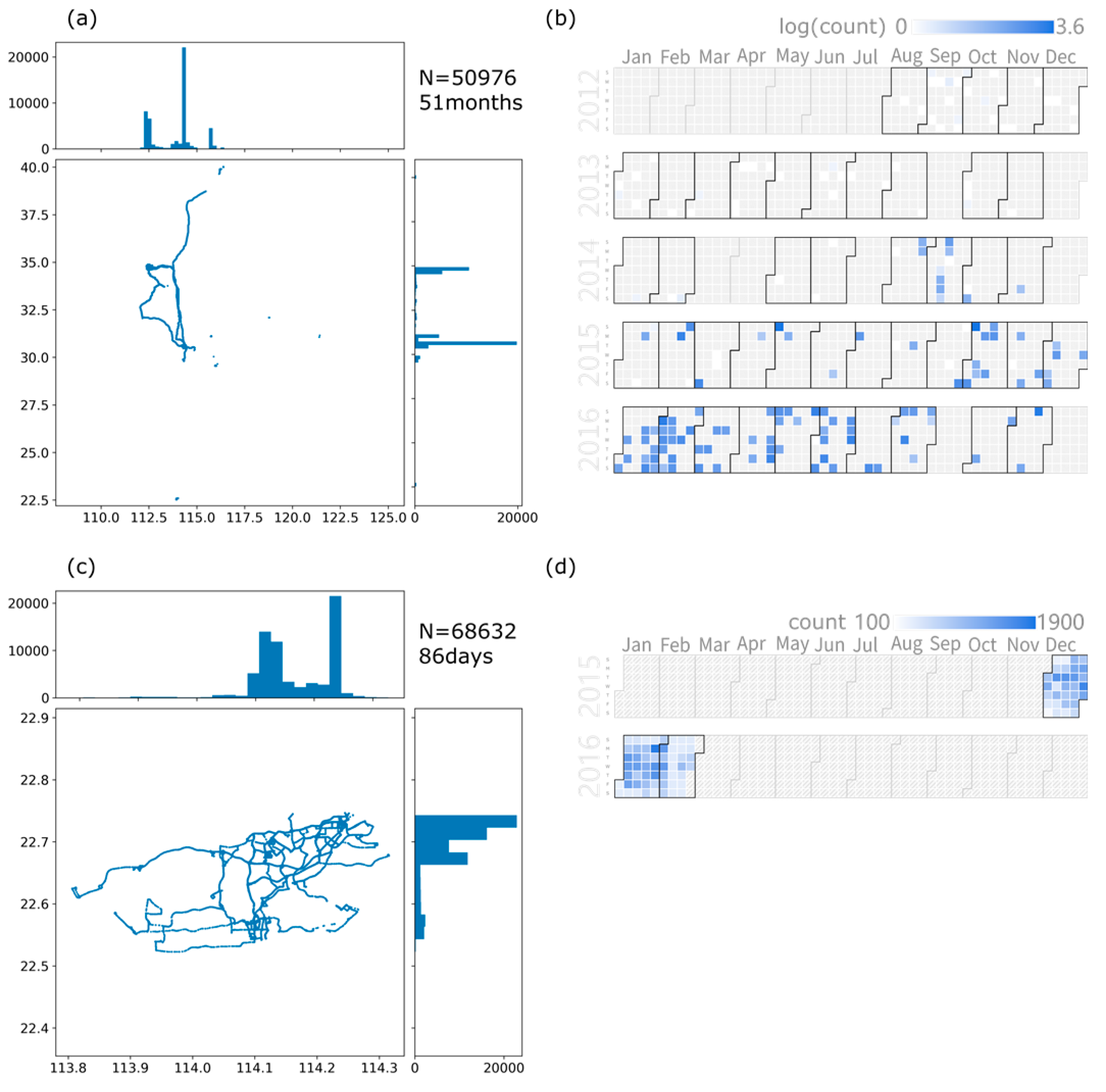
4.1. Datasets

We used two individual movement datasets with different regularity to test the proposed model. The first dataset, named student, consists of the smartphone-based GPS trajectories and the geotagged social media posts of a college student. These trajectories had a large spatial coverage (Figure 3a) but limited temporal coverage (dark cells in Figure 3b), with sampling intervals ranging from 1 s to 15 s. The trajectories involve walking and vehicle rides in daily life, as well as train rides for longer trips across the country. Geotagged social media posts were more scattered in time but less frequent (light cells in Figure 3b). Most of the trajectories were originally recorded for the purpose of voluntary map tracing instead of mobility analysis, so the missing pattern in this dataset could reflect the natural state of user generated contents.
The second dataset, named clerk, includes trajectories captured of a company employee, with sampling intervals ranging from <1 min to 5 min. Nearly 60% of the track points had sampling intervals of less than a minute, and 90% had intervals less than five minutes. This dataset was limited to one city (Figure 3c) and is more complete in the first month (Figure 3d). These trajectories captured the regular commute between home and workplace and other trips within the city for a variety of purposes.
In addition to the movement data, polygon data were also used to represent places. For the student dataset, we used administrative boundaries as a convenient tessellation choice [51], because the movement scattered over a large spatial extent and involved social media check-ins as checkpoints [52]. For the clerk dataset, we used urban road network to derive two types of zones, blocks and roads. Locations close to a road were considered to be in a road zone, while those away from roads were considered as visiting a block zone. Blocks and streets are meaningful polygonal tessellation to represent visiting and passing by places. Since there were long episodes of staying in blocks, it is necessary to differentiate staying in blocks from stops along streets, which networks cannot achieve by projecting points in blocks to adjacent segments.
Due to sparsity of the student dataset, additional travel diary was collected as ground truths for evaluation. The participant was asked to report regions he visited on specific dates guided by a collection of regional trip tickets and social media posts.

4.2. Experiment Setting

The experiment estimated and evaluated visit probability distributions using PSM-H, DRW, and TBB. These two models are both convenient to understand as baselines for comparison and representative of similar methods for the purpose of demonstrating potential problems for long gaps. Network-based models were not considered because the representation of outcomes cannot be trivially converted to areas for valid comparison. For PSM-H, the student dataset was analyzed at a daily temporal scale and spatial scale of Chinese county (administrative level below prefectural city and above township). The clerk dataset was analyzed at the temporal scale of a minute and spatial scale of urban block/street. For compared models, the maximum speed was set to 90 m/s in the regional scenario (student dataset) and 30 m/s in the urban scenario (clerk dataset).
Each movement dataset was divided into two parts: a training set as historical records for mobility pattern extraction, and a test set as ground truth for evaluation. In each test set, episodes of controlled lengths were selected as gaps for validation. For the student dataset, the training set included all trajectories and geotagged posts, with three months of travel diary as the test set. Gap lengths for tests are 7 d, 14 d, 21 d, and 28 d. For the clerk dataset, a subset of tracking data for three days was taken for test, with the rest as training data. Gap lengths for tests are 1 h, 2 h, 3 h, and 4 h. There are 44 and 40 gaps for these datasets, respectively.
We calculate a quantitative metric of how well estimated probability distributions coincide with locations that were actually visited. The hit metric for a gap g is defined as the arithmetic average of hit metric at each time unit t, i.e., hit ( g ) = | g | 1 t hit ( t ) . |g| denotes the length of the gap g. Since a ground-truth trajectory may visit multiple spatial units in one temporal unit, the hit metric for each time unit is the summation of visit probabilities of all spatial units visited in the ground truth, i.e., hit ( t ) = i G T ( t ) P ( i , t ) . GT(t) is the set of spatial units visited at time t, and P(i,t) is the probability of visiting place i at time t. For compared models, we aggregated the probability estimations for grid cells to visited polygons so that the raster-based results were comparable with polygon-based ones.

4.3. Results

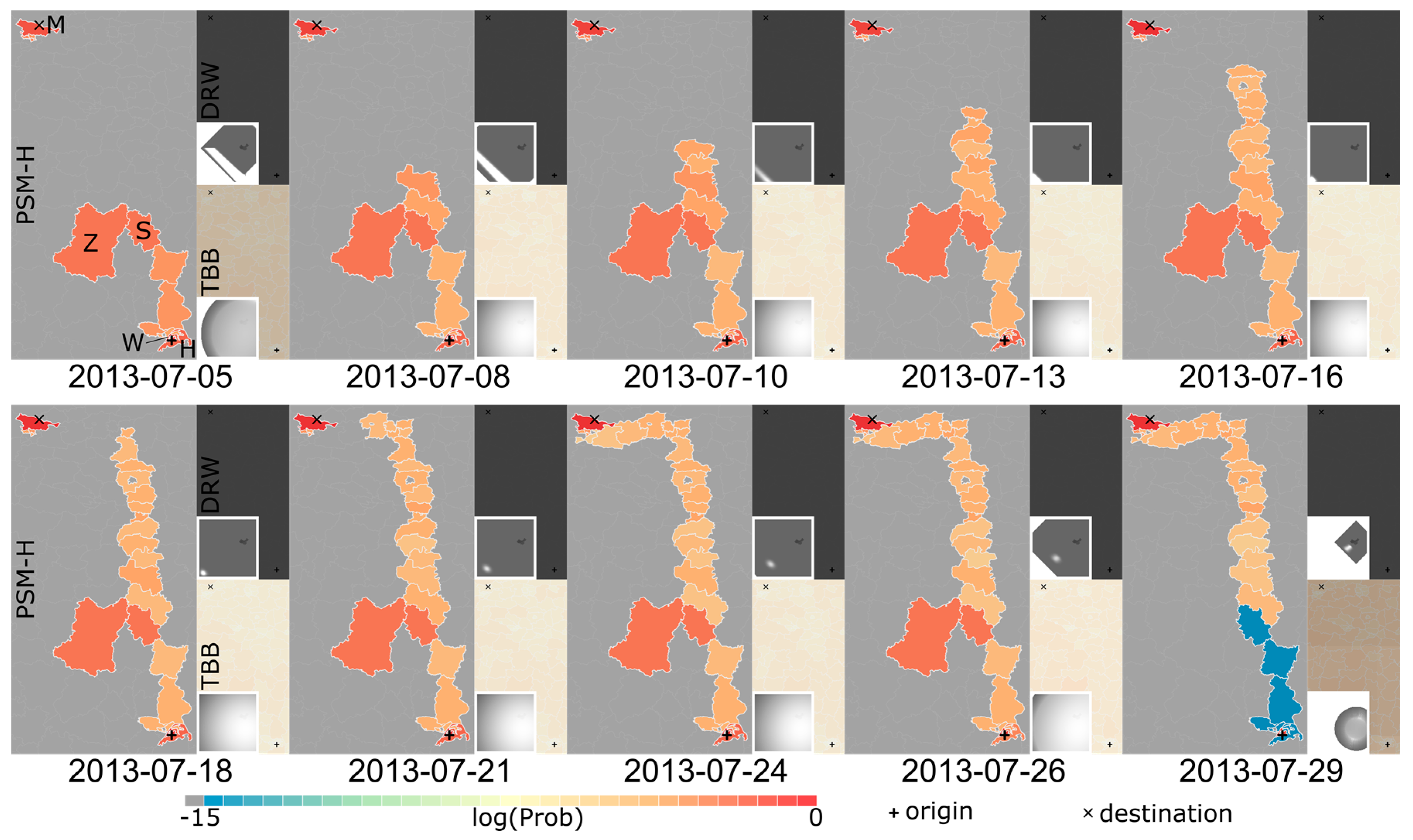
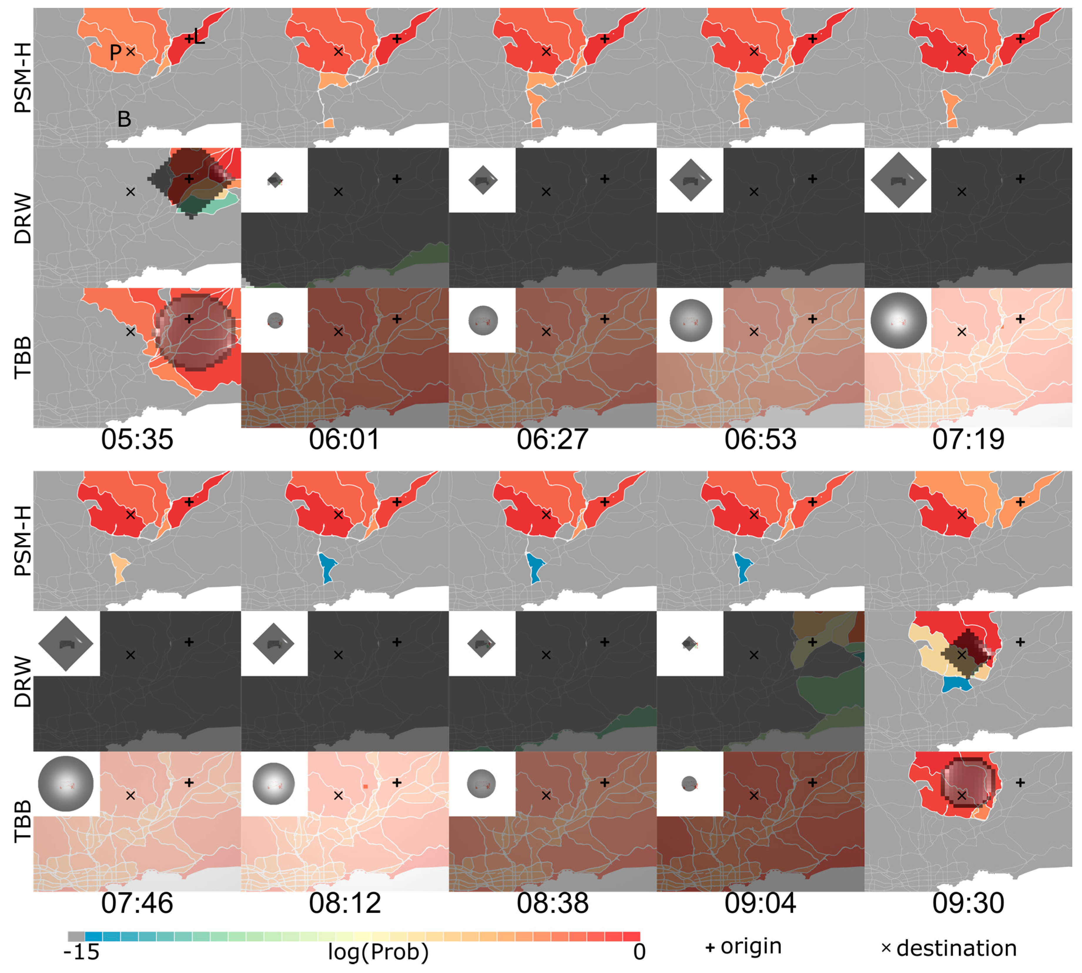
4.3.1. Visit Probability Distributions
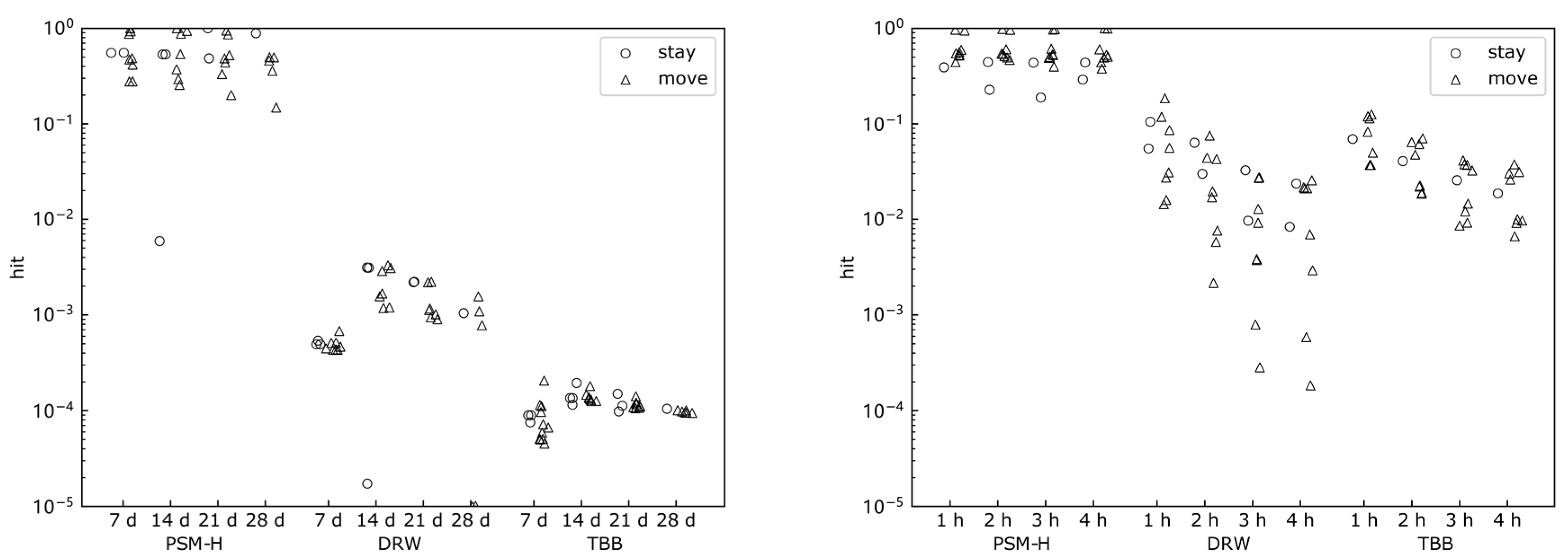
We visualized visit probability distributions for two representative gaps to seek a general sense of the model performance on long gaps. The first gap was in the student dataset, which started at Wuchang (W, university location) on July 2nd and ended at Mengjin (M, hometown location) on July 30th. The visit probabilities of places during this gap are shown in Figure 4 as a series of choropleth maps over time. The visit probabilities of W and H decreased while those for M increased before the recorded presence at hometown M. For the trip with the same origin, destination, and time budget, the visit probability distribution estimated by PSM-H was limited to a frequently visited area. The overly dispersed boundaries of DRW and TBB covered the globe given the excessive time budget and huge speed limit, which led to another problem of being truncated due to reaching the boundary of map projection.
PSM-H has also shown the ability to reflect revisits of home locations, according to highlighted significant places by different levels of probability. The highest level consists of the origin W, the destination M, and the residence H near origin. The inclusion of H in the first group confirms the pattern of visiting residence H after courses at university W. The presence of H in the gap from W to M further indicates that this pattern was taken into consideration in the estimation of unknown gaps. The middle level includes Z and S, which served as transfer stations during similar trips between college and hometown. The lowest level indicated places that frequently appeared on the paths between origin and destination. The results of compared models could only reflect linear movement, which were less realistic.
The second gap was a commute trip from home L to the workplace P from the clerk dataset, which was four hours long. The visit probabilities of urban blocks and roads for different models at ten instants during this gap are shown in Figure 5. Since this urban scenario involved a shorter period and a lower speed limit compared to the previous one, extents of the compared models were much more compact.
PSM-H captured both frequent and unusual routes by extracting mobility pattern. The blocks that a frequent commute route passed by featured visit probabilities that accumulated fast and stayed high. Some other blocks and road areas near residential area B stood out in the probability estimation, revealing an unusual detour and two intermediate blocks in commute routes. By examining the historical dataset, this unusual detour captured in mobility patterns were caused by two pick-ups at the entrance of a gated community in historical data.

4.3.2. Metrics

For PSM-H, gaps with same origin, destination, and duration are equivalent inputs, because outputs are identical visit probability distributions. Outcomes of such equivalent groups of gaps were compared to multiple ground truths, resulting in average and standard deviations of hit metrics in Table 2. As defined in Section 4.2, the hit metric was aligned to the level of polygons for the compared models. The student dataset was evaluated by 44 groups of 220 equivalent gaps from one to four weeks, while the clerk dataset was evaluated by 40 groups of 1200 equivalent gaps from one to four hours. There was a sharp contrast of numbers of ground truths for similar numbers of equivalent inputs, because movement in the student dataset was more irregular than that in the clerk dataset.
PSM-H was less sensitive to gap duration than compared models, even if PSM-H had several cases with zero hit values, which means it completely missed places that were actually visited for these origin-destination (OD) pairs. The hit metrics of PSM-H remained stable across tested gaps from two datasets, while DRW and TBB had decreasing hit metrics with increasing duration. DRW and TBB had similar hit metrics for short durations while DRW had higher hit metrics than TBB for long durations.
Different from trips from one region to another, trips starting and ending at the same region may be stationary and involve no movement at all. Considering the potential influence of these cases, we divided tested gaps into two groups by whether it started and ended at the same region. According to scatter plots in Figure 6, PSM-H had similar hit metrics for stationary and moving episodes. DRW and TBB were more likely to achieve higher hit metrics for stays than moves of the same duration.

4.4. Analysis

Hit metrics for PSM-H were at higher orders of magnitude than compared models, which was a result of compact probability distribution by incorporating mobility patterns in historical data. However, this does not mean the baseline models are not helpful as the metrics appear, with the current baseline settings of constant and extreme parameters. One must keep in mind that there are ways to improve those results by fine-tuning the speed limit parameters, given more prior knowledge about the moving individual and the transportation network in question.
To seek further understanding of the models, we analyze results reported above from the perspective of commission and omission errors [53]. Commission errors originate from predicted areas that were not visited, which was the case of vast spatial extents given by compared models for long gaps. The proposed model was able to break the link of such errors to the duration of gaps, because it limited the estimated areas to those proved possible and preferred in the past. As a result, the commission error of proposed method is only related to path diversity observed in the past. Values of hit metric indicate that the proposed method committed commission error by putting roughly half of the probability outside the visited areas due to alternative paths. This gives us a sense of how much commission error diverse paths of ordinary people may bring to the outcome of proposed method.
Meanwhile, omission errors mean that visited areas are excluded from predicted areas. Compared methods give an upper bound of accessible areas, so omission errors are not possible. Conversely, the proposed method is subject to omission errors because it is unable to capture all possible paths from a finite subset of historical paths. When one explores a new path, PSM-H will fail to hit places on it. Counts of zero values shed lights on how likely omission errors are to happen for PSM-H. Results indicate that omission errors are three months of densely sampled data were sufficient to capture most possible paths and avoid severe omission errors within a city for an ordinary clerk, although four years of sparsely geotagged social media posts were still unable to capture all possible regional movement patterns.

5. Discussion

5.1. Influence of Mobility Patterns

PSM-H is designed to model individual habits for better performance given the pervasive existence of patterns. Based on the experiment on gaps in two real datasets, we found that estimated visit probability distributions were more realistic when historical mobility patterns were considered. The proposed method relies on historical trajectories to find these patterns. In reality, the mobility pattern can vary widely across different moving objects [54,55]. It is necessary to discuss the performance when historical trajectories exhibit different patterns.
Consider two extreme cases to illustrate potential performance variation. If a person moves in a completely random manner, there is neither global preference of possible routes and schedules, nor local preference of places in neighborhood. As a result, the estimation of visit probability distribution is merely based on stay duration and travel time patterns. PSM-H falls back to reflecting space-time accessibility differences of places, which DRW depicts using combinatorics [32]. If a person has a perfectly regular routine, PSM-H is able to accurately replicate movement during gaps, because such movement leads to constant stay duration at each place and travel time between places, and deterministic distributions of routes and schedules. In other words, with the help of regularity, PSM-H reduces the size of potential area, which is key to improve accuracy [56].
The regularity of a real set of historical trajectories lies between the extremes. For example, the Geolife dataset [57] includes both irregular long trips and regular commute trips. The higher regularity historical trajectories exhibit, the better a model can perform [58]. Hence, for a generic set of historical trajectories, the performance of proposed model lies between these two extreme cases.

5.2. Choice of Spatial Units and Temporal Scales

As a fundamental issue in spatial and temporal analytics, the modifiable areal unit problem exists in the proposed model. PSM-H uses polygons (administrative regions and street/block areas) and time grains (days and minutes) as basic units. Although the choice of these units may influence the outcome [59,60], these discrete representations are beneficial for understanding movements.
Polygons facilitate the extraction of mobility patterns from noisy data by identifying visits and revisits. It helps avoid false movement metrics and patterns that measurement errors introduce [61,62], because consecutive points within a polygon is considered as a single visit despite nuances in the coordinates. When properly defined to reflect the concept of place [63], polygon representation can support semantic interpretation of trajectories [6]. In our analysis, these polygons facilitated meaningful interpretation of resident movement at regional and urban scales. In other applications, alternative spatial units can also benefit domain-specific interpretation of locations. For example, home ranges or landscape patches will make sense of animal movement [64]. In addition, these irregular polygonal tessellations are also compatible with regular grid and hexagon given proper conversion [65,66]. Discrete time enables explicit recurrence relation of visit probability surfaces as inherited from DRW [34], which allows us to apply extracted patterns to the estimation. It should be noted that there are also sophisticated alternatives to the polygon tessellation, e.g., conditional random field [67] and neural networks [12]. These methods are useful for extracting meaningful places and mapping coordinates to place representation if the bias introduced by polygon tessellation is concerned.
To minimize the side effect of discrete representation, the temporal granularity should be related to the spatial scale and the activity in question [68]. Coarse temporal granularity neglects local movements and reveals general trends [37]. Fine temporal granularity results in more stops, allowing the depiction of local routes [51]. Given the same spatial partition, the temporal scale should be finer for actively moving objects than stationary ones. There is potential periodicity in the studied movement such as diurnal or weekly repetition. It will help capture these motifs to divide one cycle into multiple temporal units [69]. For example, the analysis scales of an hour or a minute is suitable for capturing daily routines of people.

5.3. Reliability in Varied Contexts

A potential use of a visit probability model is the inference of individual movement during a data gap [70]. Such a model should work with gaps in a variety of contexts [30,71,72]. As one of its motivation, the proposed method works for trips with a wide range of length, especially long trips with different origins and destinations.
In our experiment, the context of gaps was implied by origins, destinations and time budgets. Results in Figure 6 are worth elaborating on, to shed light on the reliability of the models. The context of origins and destinations is simplified here as the relative movement states of stay and move. Ideally, there should be no differences between accuracy of stays and moves for a robust model. PSM-H performed slightly better on gaps involving moves than on stationary gaps (circles at the bottom of triangle clusters), while it is the opposite for DRW and TBB (circles at the top of triangle clusters). This means PSM-H might benefit from additional sources that may indicate the stop state [62]. In terms of time budgets, the performance of PSM-H is stable for gaps of different sizes, which supports the merit of sequence analysis used in human activity analysis [73].
The inference process of PSM-H makes use of historical data, which also requires the model to be able to face the uncertainty introduced by missing episodes. Missing data can introduce error in extracted mobility patterns. For example, missing records of stop episodes will influence the sequence frequency distribution, which can propagate to outcomes due to difference in potential routes considered by the model. Two conditions may alleviate this effect. Firstly, if gaps did not miss any stops, the sequence frequency distribution will be unaffected. Therefore, it is important to capture stops of moving object, which has been implemented in existing tracking systems [74]. Secondly, if there was a stop during a historical data gap, the actual route will lose one sample while an erroneous sample will add to a route with one stop missing. It means more samples for the OD pair will limit the effect of this sample on the sequence frequency distribution [75,76]. The development of tracking technology is promising to satisfy both conditions more easily.

5.4. Scalability for Extrapolation

The trip during a gap may involve paths never found in the past, which needs extrapolation. As an empirical model, PSM-H is limited to estimate visit probabilities of places observed in historical data, which is not suitable for the scenario of exploring new places. However, it is possible to extrapolate movement by borrowing patterns from other similar or related individuals based on social conformity principle [77]. The similarity can be measured in both geometric and semantic aspects [78], to facilitate the application of extracted patterns to a wide range of cohort.
With multiple moving objects from massive movement data, the definitions of stops, moves, routes and schedules remain the same for each individual. More agents contribute more samples to the empirical probability distributions (i.e., mobility patterns) for groups. The pattern extraction step is independent for each individual. Subsequent calculation steps are independent for each trip route and schedule. The final step is an aggregation of previous results. This design conforms to the computing paradigm of map–reduce [79], which is suitable for scalable parallel computing.

6. Conclusions

A probabilistic space-time model based on historical trajectories (PSM-H) was developed to estimate visit probability distributions during data gaps. The use of historical data results in compact spatial extents of potential areas during long gaps, which is useful to reduce commission error and keep the related omission error low for people exhibiting choice preferences.
PSM-H takes into consideration historical movement patterns such as revisits and stops derived from empirical data to extend previous time geographic probability models. Here, we use the historical movement data to characterize individual preferences, which improves upon a universal stochastic distribution for each moving object. The proposed model is suitable for inference over long periods of time, when excessive time budget renders the prediction of traditional space-time prisms (and related structures from time geography theory designed for short time spans) less informative due to the fact that they become too large in size.
By providing a way to represent and extract empirical preference in movement, the proposed model can serve as a practical tool to facilitate understanding of personal travel needs and inform future transportation plans. The output of the model, time series of visit probability distributions, can also help infer missing stops and moves during gaps in trajectory data, which improves the usability of data collected by non-professionals and enables the digital depiction of a personal travel history with imperfect data. This means digital travel surveys can include more data from digitally marginalized groups. These distributions are useful for addressing the uncertain geographical context problem when linked to environmental or other contextual information. The precise evaluation of personal risk of exposure to pollutants or pathogens will enable more effective environment management and disease prevention.

Author Contributions

Conceptualization, Chang Ren and Luliang Tang; methodology, Chang Ren; software, Chang Ren; investigation, Chang Ren; resources, Chang Ren, Luliang Tang and Jed Long; data curation, Chang Ren; writing—original draft preparation, Chang Ren, Zihan Kan; writing—review and editing, Luliang Tang, Jed Long and Xue Yang; visualization, Chang Ren; supervision, Luliang Tang and Jed Long. All authors have read and agreed to the published version of the manuscript.

Funding

This research was funded by the National Key Research and Development Program of China, grant numbers 2017YFB0503604 and 2016YFE0200400; the National Natural Science Foundation of China, grant numbers 41971405 and 41901394; China Scholarship Council, grant number 201906270227.

Data Availability Statement

The trajectory data examined in this study are available on request from the corresponding author. The data are not publicly available due to privacy restriction.

Conflicts of Interest

The authors declare no conflict of interest. The funders had no role in the design of the study; in the collection, analyses, or interpretation of data; in the writing of the manuscript, or in the decision to publish the results.

References

  1. Demšar, U.; Buchin, K.; Cagnacci, F.; Safi, K.; Speckmann, B.; Van de Weghe, N.; Weiskopf, D.; Weibel, R. Analysis and Visualisation of Movement: An Interdisciplinary Review. Mov. Ecol. 2015, 3, 1–24. [Google Scholar] [CrossRef] [PubMed] [Green Version]
  2. Kang, Y.; Gao, S.; Liang, Y.; Li, M.; Rao, J.; Kruse, J. Multiscale Dynamic Human Mobility Flow Dataset in the U.S. during the COVID-19 Epidemic. Sci. Data 2020, 7, 390. [Google Scholar] [CrossRef]
  3. Sharma, M.; Sharma, S.; Singh, G. Remote Monitoring of Physical and Mental State of 2019-NCoV Victims Using Social Internet of Things, Fog and Soft Computing Techniques. Comput. Methods Programs Biomed. 2020, 196, 105609. [Google Scholar] [CrossRef]
  4. Wan, S.; Xu, X.; Wang, T.; Gu, Z. An Intelligent Video Analysis Method for Abnormal Event Detection in Intelligent Transportation Systems. IEEE Trans. Intell. Transp. Syst. 2020, 1–9. [Google Scholar] [CrossRef]
  5. Sadilek, A.; Krumm, J. Far out: Predicting Long-Term Human Mobility. In Proceedings of the AAAI Conference on Artificial Intelligence, Toronto, ON, Canada, 22–26 July 2012; Volume 26. [Google Scholar]
  6. Parent, C.; Spaccapietra, S.; Renso, C.; Andrienko, G.; Andrienko, N.; Bogorny, V.; Damiani, M.L.; Gkoulalas-Divanis, A.; Macedo, J.; Pelekis, N.; et al. Semantic Trajectories Modeling and Analysis. ACM Comput. Surv. CSUR 2013, 45, 42. [Google Scholar] [CrossRef]
  7. Baratchi, M.; Meratnia, N.; Havinga, P.J.M.; Skidmore, A.K.; Toxopeus, B.A.K.G. A Hierarchical Hidden Semi-Markov Model for Modeling Mobility Data. In Proceedings of the 2014 ACM International Joint Conference on Pervasive and Ubiquitous Computing, Seattle, WA, USA, 13–17 September 2014; Association for Computing Machinery: New York, NY, USA, 2014; pp. 401–412. [Google Scholar]
  8. Zheng, Y.; Capra, L.; Wolfson, O.; Yang, H. Urban Computing: Concepts, Methodologies, and Applications. ACM Trans. Intell. Syst. Technol. 2014, 5, 1–55. [Google Scholar] [CrossRef]
  9. Dodge, S.; Weibel, R.; Ahearn, S.C.; Buchin, M.; Miller, J.A. Analysis of Movement Data. Int. J. Geogr. Inf. Sci. 2016, 30, 825–834. [Google Scholar] [CrossRef] [Green Version]
  10. Lee, W.-C.; Krumm, J. Trajectory Preprocessing. In Computing with Spatial Trajectories; Zheng, Y., Zhou, X., Eds.; Springer: New York, NY, USA, 2011; pp. 3–33. ISBN 978-1-4614-1629-6. [Google Scholar]
  11. Shen, L.; Stopher, P.R. Review of GPS Travel Survey and GPS Data-Processing Methods. Transp. Rev. 2014, 34, 316–334. [Google Scholar] [CrossRef]
  12. Siła-Nowicka, K.; Vandrol, J.; Oshan, T.; Long, J.A.; Demšar, U.; Fotheringham, A.S. Analysis of Human Mobility Patterns from GPS Trajectories and Contextual Information. Int. J. Geogr. Inf. Sci. 2016, 30, 881–906. [Google Scholar] [CrossRef] [Green Version]
  13. Cho, E.; Myers, S.A.; Leskovec, J. Friendship and Mobility: User Movement in Location-Based Social Networks. In Proceedings of the 17th ACM SIGKDD International Conference on Knowledge Discovery and Data Mining, San Diego, CA, USA, 21–24 August 2011; pp. 1082–1090. [Google Scholar]
  14. Rahmani, M.; Koutsopoulos, H.N. Path Inference from Sparse Floating Car Data for Urban Networks. Transp. Res. Part C Emerg. Technol. 2013, 30, 41–54. [Google Scholar] [CrossRef]
  15. Hoteit, S.; Chen, G.; Viana, A.; Fiore, M. Filling the Gaps: On the Completion of Sparse Call Detail Records for Mobility Analysis. In Proceedings of the Eleventh ACM Workshop on Challenged Networks, New York, NY, USA, 3–7 October 2016; pp. 45–50. [Google Scholar]
  16. Liu, Z.; Ma, T.; Du, Y.; Pei, T.; Yi, J.; Peng, H. Mapping Hourly Dynamics of Urban Population Using Trajectories Reconstructed from Mobile Phone Records. Trans. GIS 2018, 22, 494–513. [Google Scholar] [CrossRef]
  17. Li, M.; Gao, S.; Lu, F.; Zhang, H. Reconstruction of Human Movement Trajectories from Large-Scale Low-Frequency Mobile Phone Data. Comput. Environ. Urban Syst. 2019, 77, 101346. [Google Scholar] [CrossRef]
  18. Purves, R.S.; Laube, P.; Buchin, M.; Speckmann, B. Moving beyond the Point: An Agenda for Research in Movement Analysis with Real Data. Comput. Environ. Urban Syst. 2014, 47, 1–4. [Google Scholar] [CrossRef] [Green Version]
  19. Schafer, J.L.; Graham, J.W. Missing Data: Our View of the State of the Art. Psychol. Methods 2002, 7, 147–177. [Google Scholar] [CrossRef] [PubMed]
  20. Stovel, K.; Bolan, M. Residential Trajectories: Using Optimal Alignment to Reveal The Structure of Residential Mobility. Sociol. Methods Res. 2004, 32, 559–598. [Google Scholar] [CrossRef] [Green Version]
  21. Mayer, K.U. New Directions in Life Course Research. Annu. Rev. Sociol. 2009, 35, 413–433. [Google Scholar] [CrossRef] [Green Version]
  22. Halpin, B. Multiple Imputation for Categorical Time Series. Stata J. 2016, 16, 590–612. [Google Scholar] [CrossRef] [Green Version]
  23. Yu, S.-Z.; Kobayashi, H. A Hidden Semi-Markov Model with Missing Data and Multiple Observation Sequences for Mobility Tracking. Signal Process. 2003, 83, 235–250. [Google Scholar] [CrossRef]
  24. Crivellari, A.; Beinat, E. LSTM-Based Deep Learning Model for Predicting Individual Mobility Traces of Short-Term Foreign Tourists. Sustainability 2020, 12, 349. [Google Scholar] [CrossRef] [Green Version]
  25. Downs, J.A.; Horner, M.W. Probabilistic Potential Path Trees for Visualizing and Analyzing Vehicle Tracking Data. J. Transp. Geogr. 2012, 23, 72–80. [Google Scholar] [CrossRef]
  26. Ahearn, S.C.; Dodge, S.; Simcharoen, A.; Xavier, G.; Smith, J.L.D. A Context-Sensitive Correlated Random Walk: A New Simulation Model for Movement. Int. J. Geogr. Inf. Sci. 2017, 31, 867–883. [Google Scholar] [CrossRef]
  27. Song, Y.; Song, T.; Kuang, R. Path Segmentation for Movement Trajectories with Irregular Sampling Frequency Using Space-Time Interpolation and Density-Based Spatial Clustering. Trans. GIS 2019, 23, 558–578. [Google Scholar] [CrossRef]
  28. Loraamm, R.W. Incorporating Behavior into Animal Movement Modeling: A Constrained Agent-Based Model for Estimating Visit Probabilities in Space-Time Prisms. Int. J. Geogr. Inf. Sci. 2020, 34, 1607–1627. [Google Scholar] [CrossRef]
  29. An, L.; Tsou, M.-H.; Crook, S.E.; Chun, Y.; Spitzberg, B.; Gawron, J.M.; Gupta, D.K. Space–Time Analysis: Concepts, Quantitative Methods, and Future Directions. Ann. Assoc. Am. Geogr. 2015, 105, 891–914. [Google Scholar] [CrossRef]
  30. Kwan, M.-P. The Uncertain Geographic Context Problem. Ann. Assoc. Am. Geogr. 2012, 102, 958–968. [Google Scholar] [CrossRef]
  31. Miller, H.J. Time Geography and Space-Time Prism. In The International Encyclopedia of Geography; Wiley: Hoboken, NJ, USA, 2016. [Google Scholar]
  32. Winter, S.; Yin, Z.-C. Directed Movements in Probabilistic Time Geography. Int. J. Geogr. Inf. Sci. 2010, 24, 1349–1365. [Google Scholar] [CrossRef]
  33. Winter, S.; Yin, Z.-C. The Elements of Probabilistic Time Geography. GeoInformatica 2011, 15, 417–434. [Google Scholar] [CrossRef]
  34. Song, Y.; Miller, H.J. Simulating Visit Probability Distributions within Planar Space-Time Prisms. Int. J. Geogr. Inf. Sci. 2014, 28, 104–125. [Google Scholar] [CrossRef]
  35. Long, J.A.; Nelson, T.A.; Nathoo, F.S. Toward a Kinetic-Based Probabilistic Time Geography. Int. J. Geogr. Inf. Sci. 2014, 28, 855–874. [Google Scholar] [CrossRef] [Green Version]
  36. Song, Y.; Miller, H.J.; Zhou, X.; Proffitt, D. Modeling Visit Probabilities within Network-Time Prisms Using Markov Techniques. Geogr. Anal. 2016, 48, 18–42. [Google Scholar] [CrossRef]
  37. Gonzalez, M.C.; Hidalgo, C.A.; Barabasi, A.-L. Understanding Individual Human Mobility Patterns. Nature 2008, 453, 779–782. [Google Scholar] [CrossRef]
  38. Abbott, A. Sequence Analysis: New Methods for Old Ideas. Annu. Rev. Sociol. 1995, 21, 93–113. [Google Scholar] [CrossRef]
  39. Gauthier, J.-A.; Bühlmann, F.; Blanchard, P. Introduction: Sequence Analysis in 2014. In Advances in Sequence Analysis: Theory, Method, Applications; Blanchard, P., Bühlmann, F., Gauthier, J.-A., Eds.; Life Course Research and Social Policies; Springer International Publishing: Cham, Switzerland, 2014; pp. 1–17. ISBN 978-3-319-04969-4. [Google Scholar]
  40. Gabadinho, A.; Ritschard, G.; Studer, M.; Müller, N.S. Extracting and Rendering Representative Sequences. In Knowledge Discovery, Knowlege Engineering and Knowledge Management; Fred, A., Dietz, J.L.G., Liu, K., Filipe, J., Eds.; Springer: Berlin/Heidelberg, Germany, 2011; pp. 94–106. [Google Scholar]
  41. Barban, N.; Billari, F.C. Classifying Life Course Trajectories: A Comparison of Latent Class and Sequence Analysis. J. R. Stat. Soc. Ser. C Appl. Stat. 2012, 61, 765–784. [Google Scholar] [CrossRef]
  42. Baumann, P.; Kleiminger, W.; Santini, S. How Long Are You Staying? Predicting Residence Time from Human Mobility Traces. In Proceedings of the 19th Annual International Conference on Mobile Computing & Networking, Miami, FL, USA, 30 September–4 October 2013; pp. 231–234. [Google Scholar]
  43. Wei, L.-Y.; Zheng, Y.; Peng, W.-C. Constructing Popular Routes from Uncertain Trajectories. In Proceedings of the 18th ACM SIGKDD International Conference on Knowledge Discovery and Data Mining, Beijing, China 12–16 August 2012; pp. 195–203. [Google Scholar]
  44. Su, H.; Zheng, K.; Wang, H.; Huang, J.; Zhou, X. Calibrating Trajectory Data for Similarity-Based Analysis. In Proceedings of the 2013 ACM SIGMOD International Conference on Management of Data, New York, NY, USA, 22–27 June 2013; pp. 833–844. [Google Scholar]
  45. Luo, W.; Tan, H.; Chen, L.; Ni, L.M. Finding Time Period-Based Most Frequent Path in Big Trajectory Data. In Proceedings of the 2013 ACM SIGMOD International Conference on Management of Data, New York, NY, USA, 22–27 June 2013; pp. 713–724. [Google Scholar]
  46. Huang, Q. Mining Online Footprints to Predict User’s next Location. Int. J. Geogr. Inf. Sci. 2017, 31, 523–541. [Google Scholar] [CrossRef]
  47. Zheng, K.; Zheng, Y.; Xie, X.; Zhou, X. Reducing Uncertainty of Low-Sampling-Rate Trajectories. In Proceedings of the 2012 IEEE 28th International Conference on Data Engineering, Arlington, VA, USA, 1–5 April 2012; pp. 1144–1155. [Google Scholar]
  48. Baratchi, M.; Meratnia, N.; Havinga, P.J. Finding Frequently Visited Paths: Dealing with the Uncertainty of Spatio-Temporal Mobility Data. In Proceedings of the 2013 IEEE Eighth International Conference on Intelligent Sensors, Sensor Networks and Information Processing, Melbourne, Australia, 2–5 April 2013; pp. 479–484. [Google Scholar]
  49. Huang, Q.; Wong, D.W. Modeling and Visualizing Regular Human Mobility Patterns with Uncertainty: An Example Using Twitter Data. Ann. Assoc. Am. Geogr. 2015, 105, 1179–1197. [Google Scholar] [CrossRef]
  50. Daintith, J.; Wright, E. Run-length encoding. In A Dictionary of Computing; Oxford University Press: Oxford, UK, 2008; ISBN 978-0-19-923400-4. [Google Scholar]
  51. Du Mouza, C.; Rigaux, P. Multiscale Classification of Moving Objects Trajectories. In Proceedings of the 16th International Conference on Scientific and Statistical Database Management, Santorini Island, Greece, 21–23 June 2004; pp. 307–316. [Google Scholar]
  52. Tao, Y.; Both, A.; Duckham, M. Analytics of Movement through Checkpoints. Int. J. Geogr. Inf. Sci. 2018, 32, 1282–1303. [Google Scholar] [CrossRef]
  53. Long, J.A.; Nelson, T.A. Time Geography and Wildlife Home Range Delineation. J. Wildl. Manag. 2012, 76, 407–413. [Google Scholar] [CrossRef] [Green Version]
  54. Jiang, S.; Ferreira, J.; González, M.C. Clustering Daily Patterns of Human Activities in the City. Data Min. Knowl. Discov. 2012, 25, 478–510. [Google Scholar] [CrossRef] [Green Version]
  55. Long, Y.; Liu, X.; Zhou, J.; Chai, Y. Early Birds, Night Owls, and Tireless/Recurring Itinerants: An Exploratory Analysis of Extreme Transit Behaviors in Beijing, China. Habitat Int. 2016, 57, 223–232. [Google Scholar] [CrossRef] [Green Version]
  56. Furtado, A.S.; Alvares, L.O.C.; Pelekis, N.; Theodoridis, Y.; Bogorny, V. Unveiling Movement Uncertainty for Robust Trajectory Similarity Analysis. Int. J. Geogr. Inf. Sci. 2018, 32, 140–168. [Google Scholar] [CrossRef]
  57. Zheng, Y.; Xie, X.; Ma, W.-Y. GeoLife: A Collaborative Social Networking Service among User, Location and Trajectory. IEEE Data Eng. Bull. 2010, 33, 32–40. [Google Scholar]
  58. Song, C.; Qu, Z.; Blumm, N.; Barabási, A.-L. Limits of Predictability in Human Mobility. Science 2010, 327, 1018–1021. [Google Scholar] [CrossRef] [Green Version]
  59. Openshaw, S. Ecological Fallacies and the Analysis of Areal Census Data. Environ. Plan. Econ. Space 1984, 16, 17–31. [Google Scholar] [CrossRef] [PubMed] [Green Version]
  60. Cheng, T.; Adepeju, M. Modifiable Temporal Unit Problem (MTUP) and Its Effect on Space-Time Cluster Detection. PLoS ONE 2014, 9, e100465. [Google Scholar] [CrossRef] [Green Version]
  61. Laube, P.; Purves, R.S. How Fast Is a Cow? Cross-Scale Analysis of Movement Data. Trans. GIS 2011, 15, 401–418. [Google Scholar] [CrossRef]
  62. Hwang, S.; VanDeMark, C.; Dhatt, N.; Yalla, S.V.; Crews, R.T. Segmenting Human Trajectory Data by Movement States While Addressing Signal Loss and Signal Noise. Int. J. Geogr. Inf. Sci. 2018, 32, 1391–1412. [Google Scholar] [CrossRef] [Green Version]
  63. Goodchild, M.F. Formalizing Place in Geographic Information Systems. In Communities, Neighborhoods, and Health: Expanding the Boundaries of Place; Burton, L.M., Matthews, S.A., Leung, M., Kemp, S.P., Takeuchi, D.T., Eds.; Social Disparities in Health and Health Care; Springer: New York, NY, USA, 2011; pp. 21–33. ISBN 978-1-4419-7482-2. [Google Scholar]
  64. Revilla, E.; Wiegand, T. Individual Movement Behavior, Matrix Heterogeneity, and the Dynamics of Spatially Structured Populations. Proc. Natl. Acad. Sci. USA 2008, 105, 19120–19125. [Google Scholar] [CrossRef] [Green Version]
  65. Huber, D.L.; Church, R.L. Transmission Corridor Location Modeling. J. Transp. Eng. 1985, 111, 114–130. [Google Scholar] [CrossRef]
  66. Shirabe, T. A Method for Finding a Least-Cost Wide Path in Raster Space. Int. J. Geogr. Inf. Sci. 2016, 30, 1469–1485. [Google Scholar] [CrossRef]
  67. Liao, L.; Fox, D.; Kautz, H. Extracting Places and Activities from GPS Traces Using Hierarchical Conditional Random Fields. Int. J. Robot. Res. 2007, 26, 119–134. [Google Scholar] [CrossRef]
  68. Meentemeyer, V. Geographical Perspectives of Space, Time, and Scale. Landsc. Ecol. 1989, 3, 163–173. [Google Scholar] [CrossRef]
  69. Schneider, C.M.; Belik, V.; Couronné, T.; Smoreda, Z.; González, M.C. Unravelling Daily Human Mobility Motifs. J. R. Soc. Interface 2013, 10, 20130246. [Google Scholar] [CrossRef] [Green Version]
  70. Kuijpers, B.; Othman, W. Modeling Uncertainty of Moving Objects on Road Networks via Space-Time Prisms. Int. J. Geogr. Inf. Sci. 2009, 23, 1095–1117. [Google Scholar] [CrossRef]
  71. Timmermans, H.J.P.; Zhang, J. Modeling Household Activity Travel Behavior: Examples of State of the Art Modeling Approaches and Research Agenda. Transp. Res. Part B Methodol. 2009, 43, 187–190. [Google Scholar] [CrossRef]
  72. Avgar, T.; Mosser, A.; Brown, G.S.; Fryxell, J.M. Environmental and Individual Drivers of Animal Movement Patterns across a Wide Geographical Gradient. J. Anim. Ecol. 2013, 82, 96–106. [Google Scholar] [CrossRef]
  73. Shoval, N.; Isaacson, M. Sequence Alignment as a Method for Human Activity Analysis in Space and Time. Ann. Assoc. Am. Geogr. 2007, 97, 282–297. [Google Scholar] [CrossRef]
  74. Kjærgaard, M.B.; Bhattacharya, S.; Blunck, H.; Nurmi, P. Energy-Efficient Trajectory Tracking for Mobile Devices. In Proceedings of the 9th International Conference on Mobile Systems, Applications, and Services, Bethesda, MD, USA, 28 June–1 July 2011; pp. 307–320. [Google Scholar]
  75. Greenwood, J.A.; Sandomire, M.M. Sample Size Required for Estimating the Standard Deviation as a Per Cent of Its True Value. J. Am. Stat. Assoc. 1950, 45, 257–260. [Google Scholar] [CrossRef]
  76. Seaman, D.E.; Millspaugh, J.J.; Kernohan, B.J.; Brundige, G.C.; Raedeke, K.J.; Gitzen, R.A. Effects of Sample Size on Kernel Home Range Estimates. J. Wildl. Manag. 1999, 63, 739–747. [Google Scholar] [CrossRef]
  77. Wang, Y.; Yuan, N.J.; Lian, D.; Xu, L.; Xie, X.; Chen, E.; Rui, Y. Regularity and Conformity: Location Prediction Using Heterogeneous Mobility Data. In Proceedings of the 21th ACM SIGKDD International Conference on Knowledge Discovery and Data Mining, Sydney, Australia, 10–13 August 2015; pp. 1275–1284. [Google Scholar]
  78. Miller, J.C. Embodied Architectural Geographies of Consumption and the Mall Paseo Chiloe Controversy in Southern Chile. Ann. Am. Assoc. Geogr. 2019, 109, 1300–1316. [Google Scholar] [CrossRef]
  79. Dean, J.; Ghemawat, S. MapReduce: Simplified Data Processing on Large Clusters. Commun. ACM 2008, 51, 107–113. [Google Scholar] [CrossRef]
Figure 1. Representation of trajectories for the mobility pattern extraction.(a) A trajectory passes by areas from A to D. (b) The trajectory is represented as discrete area labels and corresponding time. (c) The consecutive stay in each area is considered as an episode in run-length encoding scheme. The length of horizontal line represents its duration. An episode is considered as a stop if it is longer than the time scale τ (capped lines), otherwise a move. (d) The trajectory is represented as a sequence of areas with stop (solid dot) or move (open dot) labels. (e) Corresponding data representations for (a) to (d).
Ijgi 10 00456 g001
Figure 2. Possible routes and schedules during a gap. (a) Two possible routes from origin + to destination × indicated by historical data. (b) Multiple possible schedules for route R1 (upper) and R2 (lower). The horizontal axis is time and the vertical axis is places along each route. Horizontal lines represent stays at a place and inclined lines represent moves between places. (c) Sliding windows of schedule S2,4 on a gap that is much longer than the schedule. The first row shows S2,4 as a discrete sequence of places. Each of the rows below moves the sequence by one time unit along the gap, and the schedule is padded (grey) with origin on the left and destination on the right.
Ijgi 10 00456 g002
Figure 3. The spatiotemporal distribution of the datasets (a) Trajectories collected by smartphone and social media check-ins of a student in Central China. Top and right panels are one-dimensional histograms of point coordinates. (b) Temporal distributions of student dataset, shading is proportional to the logarithm of number of data points collected in a day. (c) Trajectories collected by private car of an employee in Shenzhen, China. (d) Temporal distributions of clerk dataset, shading is proportional to the number of data points collected in a day.
Ijgi 10 00456 g003
Figure 4. The visit probability distributions by four models during a long trajectory gap involving a regional trip. The extent of each snapshot is 30.27N to 35.08N, and 112.15E to 114.70E, while that of each inset is 85.06S to 85.06N, and 180.0W to 180.0E.
Ijgi 10 00456 g004
Figure 5. The visit probability distributions by four models during a trajectory gap involving an urban trip. There are ten groups of snapshots of the dynamic probability distribution. The extent of each snapshot is 22.52N to 22.79N, and 113.94E to 114.34E, while that of each inset is 20.84N to 24.57N, and 112.11E to 116.27E.
Ijgi 10 00456 g005
Figure 6. Hit metrics for stationary and moving episodes Left: student dataset, right: clerk dataset.
Ijgi 10 00456 g006
Table 1. List of symbols.
SymbolDescriptionSymbolDescription
pidlid of l-th placeJtotal number of points
polygonlgeometry of l-th polygonKnumber of MLE episodes
<xj, yj, tj>geographic coordinates and timestamp of j-th pointLtotal number of defined places
Nknumber of location fixes in an MLE episodeMtotal number of stops
tsk, tekstart and end time of k-th episodeNtotal number of moves
sidmid of m-th stop episodeRset of place subsequence representing stops between a pair of places
spidmplace id associated with m-th stop episoder, r’sample stop sequences from set R
midnid of n-th move episodeSset of place subsequences representing paths between a pair of places
pidon, piddnplace ids of the origin and destination of n-th move episodessample paths from set S
ton, tdntimes at the origin and destination of n-th move episodesu, su’u-th and u’-th place from path s
a, b, i, i’sample place idsAC(a,b)count of adjacent occurrence of places a and b
o, dplace id of origin and destinationSDs;a)frequency distribution of stay duration Δs at place a
Δsduration of a stop episodeTTt;a,b)frequency distribution of travel time Δt from place a to b
Δtduration of a move episodeSF(r)frequency distribution of stop sequence r for a trip
spid[m,m’]subsequence of sequence spid from m-th to m’-th elementMD(a,b|o,d)count of occurrence of place a ahead of b for a trip from place o to d
|∙|cardinality operator, number of elements in a set{element| condition}a set of elements satisfying condition specified after the vertical bar
^logical ‘and’ operator
Table 2. Hit metrics of visit probability estimated by three models in two datasets.
Student DatasetClerk Dataset
ΔT7 d14 d21 d28 d60 min120 min180 min240 min
N(OD)141211710101010
N0(OD) 142211000
PSM-H42% ± 35%45% ± 36%48% ± 35%41% ± 28%55% ± 27%58% ± 23%56% ± 24%57% ± 24%
DRW0.04% ± 0.02%0.20% ± 0.12%0.13% ± 0.08%0.06% ± 0.06%7% ± 5%3% ± 3%1% ± 1%1% ± 1%
TBB0.01% ± 0.00%0.01% ± 0.00%0.01% ± 0.00%0.01% ± 0.00%8% ± 4%4% ± 2%2% ± 1%2% ± 1%
1 Number of OD pairs for which PSM-H achieved zero hit.
Publisher’s Note: MDPI stays neutral with regard to jurisdictional claims in published maps and institutional affiliations.

