
Gaussian Process Regression-Based Structural Response Model and Its Application to Regional Damage Assessment


1
Department of Structural Engineering Research, Korea Institute of Civil Engineering and Building Technology, Goyang-si 10223, Gyeonggi-do, Korea
2
Division for Integrated Water Management, Korea Environment Institute, Sejong 30147, Korea
*
Author to whom correspondence should be addressed.
ISPRS Int. J. Geo-Inf. 2021, 10(9), 574; https://0-doi-org.brum.beds.ac.uk/10.3390/ijgi10090574
Submission received: 29 June 2021
/
Revised: 17 August 2021
/
Accepted: 20 August 2021
/
Published: 24 August 2021
/
Corrected: 6 January 2022
(This article belongs to the Special Issue Geomatics and Geo-Information in Earthquake Studies)
Abstract
:Seismic activities are serious disasters that induce natural hazards resulting in an incalculable amount of damage to properties and millions of deaths. Typically, seismic risk assessment can be performed by means of structural damage information computed based on the maximum displacement of the structure. In this study, machine learning models based on GPR are developed in order to estimate the maximum displacement of the structures from seismic activities and then used to construct fragility curves as an application. During construction of the models, 13 features of seismic waves are considered, and six wave features are selected to establish the seismic models with the correlation analysis normalizing the variables with the peak ground acceleration. Two models for six-floor and 13-floor buildings are developed, and a sensitivity analysis is performed to identify the relationship between prediction accuracy and sampling size. A 10-fold cross-validation method is used to evaluate the model performance, using the R-squared, root mean squared error, Nash criterion, and mean bias. Results of the six-parameter-based model apparently indicate a similar performance to that of the 13-parameter-based model for the two types of buildings. The model for the six-floor building affords a steadily enhanced performance by increasing the sampling size, while the model for the 13-floor building shows a significantly improved performance with a sampling size of over 200. The results indicate that the heighted structure requires a larger sampling size because it has more degrees of freedom that can influence the model performance. Finally, the proposed models are successfully constructed to estimate the maximum displacement, and applied to obtain fragility curves with various performance levels. Then, the regional seismic damage is assessed in Gyeonjgu city of South Korea as an application of the developed models. The damage assessment with the fragility curve provides the structural response from the seismic activities, which can assist in minimizing damage.
1. Introduction
Assessment of seismic building damage has played a significant role in establishing the earthquake model frameworks with enhanced performances. Moreover, the seismic probabilistic risk assessment (SPRA) with the maximum displacement estimation in residential buildings is a crucial step in the improvement of model performances. Based on the model, prompt structural responses can be provided to reduce damages from natural disasters such as earthquakes [1,2,3]. Iervolino and Giorgio [4] investigated building levels, which are related to the degree of freedom in a structure, to identify the limitation of the building level using the functionality level for a seismic damage. Burton et al. [5] analyzed functionality and recovery post-earthquake based on the building-level limit states which are applied for optimization of a structure and lifecycle seismic performance assessment.
Fragility curves are commonly used for seismic vulnerability assessment by linking the probability of exceedance of the limit states to ground shaking intensity in order to provide structural response. To obtain fragility curves, empirical and analytical fragility investigations can be carried out using data/information on past damages from earthquakes and structural properties correlated with seismic activities. The analytical fragility approach has been commonly used in estimating fragility curves for seismic analysis, because the data on structural damage is generally insufficient for the application of the empirical fragility approach [6,7]. In the fragility analysis, it is important to calculate the accurate maximum displacement, which represents the earthquake response of a building and to estimate the performance of the structure affected by seismic excitations [2]. The seismic fragility analysis can be enhanced by developing the SPRA with an application of the information derived from the earthquake occurrence. SPRA is examined based on a conditional probability, where the measure of the damage exceeds a threshold at a given intensity measure of a structure [8]. Characteristics of structures can be used to determine structure activities and to assess structural safety for the analysis by SPRA using numerical analysis, applied to estimate structural fragility and assess the risk of collapse [9,10,11].
Furthermore, several methodologies have been utilized to improve the maximum displacement estimation that produces the seismic fragility curve for the responses of natural disasters. Machine learning techniques, including an artificial neural network, an integrated fuzzy analytic hierarchy process, and machine learning-based regression models, were applied for the evaluation of earthquake damages [12,13,14]. Lagaros and Fragiadakis [15] used neural networks to conduct a fragility assessment based on steel frames with seismic activities. Unnikrishnan et al. [16] examined fragility curves using a high-dimensional model that decomposes the nonlinear relationship between input and output variables. Saha et al. [17] used a polynomial regression model to analyze the maximum displacement. Calabrese and Lai [18] and Gehl and D’Ayala [19] applied the artificial neural networks and Bayesian networks for the multi-risk fragility analysis in seismic models. More recently, Jung et al. [20] proposed the application of a Gaussian process regression (GPR) method, wherein they compared various approaches in estimating the maximum displacement to provide fragility curves for prompt response from natural disasters. In the analysis, the maximum inter-story drift ratio (MIDR) was used to create the fragility curve for the seismic vulnerability assessment.
The Korean Peninsula is located in East Asia, surrounded by the Eurasian plate where earthquakes occur. This peninsula has landscapes including plutonic, sedimentary, and volcanic rocks deposited over a tectonic and geomorphic history [21] and geological structures including faults and weak crust that have led to concurrent earthquakes [22]. Mountain ranges on the peninsula are featured by erosions and tectonic movements with an asymmetric topography that has experienced an initial uplift [23]. One of main regions in the Korean Peninsula affected by seismic activities is Gyeongju, which has suffered from numerous casualties and damages. For example, the Gyeongju Earthquake, with a local magnitude (ML) of 5.8 in 2016, occurred five months after the Kumamoto Earthquake, which had a magnitude (ML) of 7.3 [24]. The earthquake was preceded by a foreshock with an ML of 5.1, and it induced 601 aftershocks. This earthquake caused damage to 5368 properties, injured 23 people, and subsequently, resulted in 111 casualties in the area. Although significant national losses have occurred from continuous damages caused by seismic activities in the peninsula, vulnerability assessment analyses for different types of buildings in the region, based on advanced seismic models, to reduce potential losses have been scarce.
This study aimed to develop advanced and robust models for estimating the maximum displacement to earthquakes. Additionally, the proposed model must help assess the structural vulnerability to natural disasters by means of fragility curves. In this study, the model was applied to the Gyeongju region to examine regional seismic damage assessment. For this purpose, the input variables in the model framework were identified using the correlation analysis with various seismic magnitudes and waves. A machine learning technique was applied for a six-floor building and a 13-floor building to improve the estimation models. The proposed models are based on the peak ground acceleration (PGA). Different sampling sets, such as 100, 150, 200, 250, 300, 350, and 400, for the number of the waves were investigated to determine the appropriate sampling size in establishing the models using various statistical indices.
2. Methodology
2.1. Estimation Model Based on Gaussian Process Regression
In this study, we employed GPR (also known as Kriging) to develop a seismic model and to analyze the model performance in estimating the maximum displacement of the structure and the seismic fragility curves. GPR analysis is a type of regression analysis that is adopted when the dependent variable follows the Gaussian process [20,25,26]. Phan et al. [27] and Hoang et al. [28] used the GPR technique for seismic vulnerability and seismic fragility analysis for storage tanks and reinforced concrete highway bridges. Jung et al. [20] also investigated several methods in estimating the maximum displacement and found that the GPR approach showed the best performance. GPR has the structural characteristic of machine learning techniques, assuming that the model output, Y(x), indicates a realization of a Gaussian process. The formulation of the model can be obtained as follows:
where Y(x) means the unknown function of interest, indicates a vector of unknown repression coefficient, f(x) implies a vector of known regression function, and Z(x) is a realization of the Gaussian process based on zero mean and nonzero covariance. The Z(x) can be expressed as
where indicates the process variance and implies the spatial correlation function using unknown and known correlation parameters . The correlation between and means the function of a distance between and . The output, , of the model can be obtained using the input points and the corresponding computer output . The related equation can be formulated as
where is the regression function vector for the estimated data and is the regression function matrix of the training data. is the vector of the correlation function between and and indicates the correlation matrix of . The model can interpolate the n data points based on the various basic functions and correlation functions. With Equation (3), the best linear unbiased predictor of can be gained as follows:
Additionally, the mean standardized error for the estimate, , can be obtained from
The unknown parameter () should be estimated to obtain the model by solving an optimization problem. The maximum likelihood estimation approach is used to determine the parameters (, , and ) maximizing the quantity in Equation (3). The input variables and the output variable derived from the model are described in Section 3.1. The cross-validation method considering the training data and testing data for the model process is explained in Section 2.3. A comprehensive description of the GPR procedure was presented by Williams and Rasmussen [29].
2.2. Seismic Probabilistic Risk Assessment
Once the maximum displacement is estimated using the GPR method, the seismic probability risk assessment can be performed based on the seismic fragility curve. The fragility curve is applied for the structural safety analysis [30]. These curves can be used to evaluate seismic structural performance and obtain the probability of a structure’s safety or failure against natural disasters.
To generate the fragility curve, we performed a simulation analysis by increasing the magnitude of earthquakes in buildings. Then, the maximum displacement derived from the simulation was validated using the immediate occupancy (IO), life safety (LS), and collapse prevention (CP) levels. With the maximum displacement, the fragility curve is expressed as a log-normal distribution function, which can indicate the probability of seismic damages related to seismic intensity. The distribution function within the intensity ranges implies the function of the seismic intensity, indicating the performance of the seismic analysis. In the analysis, the maximum likelihood estimation method is used to obtain statistical parameters of the fragility curve, i.e., mean and standard deviation of log-normal distribution function. The maximum likelihood function can be expressed as follows:
where represents the fragility curve generated from the maximum displacement and implies the seismic intensity, the peak ground acceleration (PGA) adopted in this study. Here, if a seismic damage occurs at the ith site, whereas when there is no damage to a structure. N indicates the total number of sites observed for the investigation. In the equation, can be written as follows based on the following log-normal assumption:
where represents the PGA, c denotes the median value in the fragility curve, ζ indicates the standard deviation of the curve, and Φ[∙] denotes the function of the standardized normal distribution.
2.3. Evaluation Criteria
To evaluate the model performance, cross-validation resampling techniques have been commonly used by comparing observed variables with estimated variables [20,31,32,33]. In this study, the k-fold cross-validation approach is applied for validating the displacement estimation by obtaining boundaries of errors and estimated errors [34]. When k represents a value of 10 as used in this study, 10% of the data are temporarily excluded for testing and the remaining data is used for training by structuring a model. In other words, the data are divided into 10 groups of the same or similar size. One of the groups is designated as the test set, and remaining groups are used for the training set. Each group is repeatedly excluded in the 10 groups considering the error variability. The estimated displacement is then evaluated based on statistical indices with the measured displacement to conduct a model performance analysis. Several studies were conducted for sensitivity analysis based on k-fold cross-validation, including 10-fold cross-validation [35,36]. This 10-fold cross validation was also used in this study because other cross-validation methods, such as Jackknife, apparently reduce the accuracy of the model owing to the large number of data sets.
The evaluation methods employing statistical analysis used in the study are the R-squared (R2), the root mean squared error (RMSE), the Nash criterion (NASH), and the mean bias (BIAS). We attempted to evaluate the estimated values based on four criteria—R2, RMSE, NASH, and BIAS. These criteria can assess the accuracy and bias of the model’s results. In this study, we used the RMSE for the model accuracy instead of the MAE, because the RMSE were applied for the evaluation of model performance in several studies as one of the general methods in evaluation criteria [20,32,37,38]. The indices are calculated using the following equations:
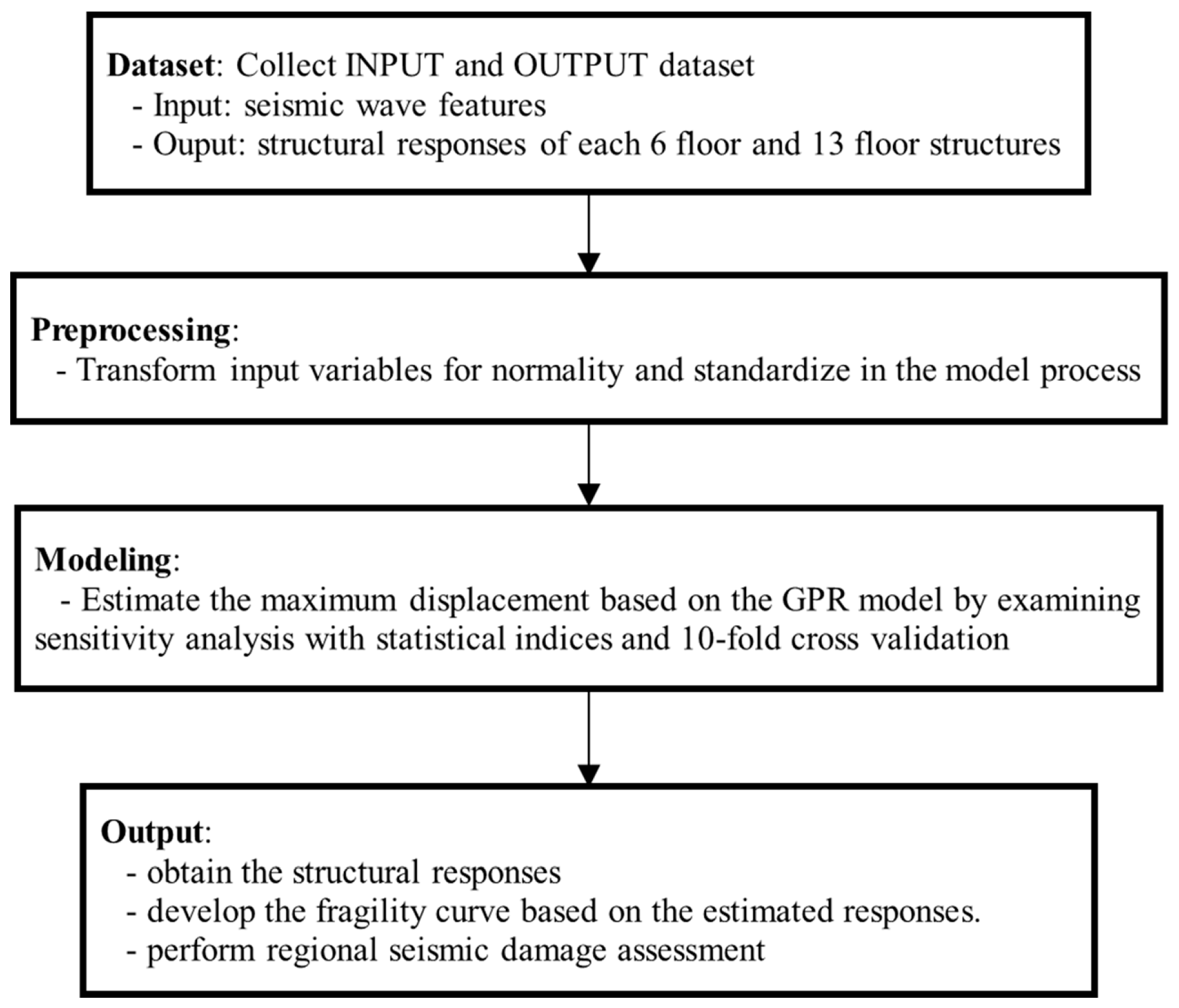
where RSS is the residual sum of squares and TSS is the total sum of squares. The total number of data is expressed as n, the at-site estimate for location i is denoted as , and the estimate based on the proposed model for location i is presented as . A simple diagram for estimating the maximum displacement and obtaining the fragility curves is shown in Figure 1.
3. Data Set
3.1. Feature Selection of Seismic Waves
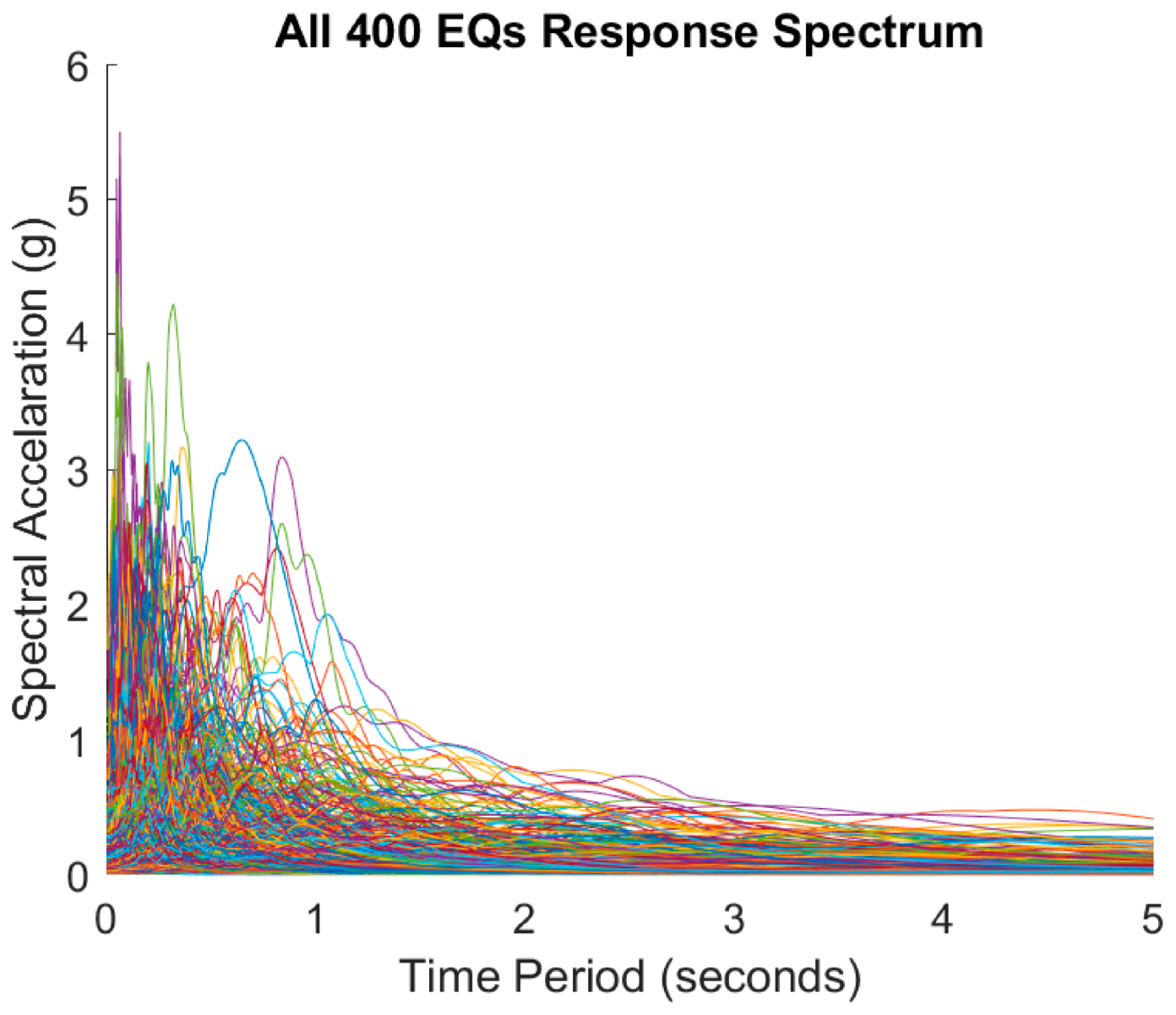
Thirteen seismic wave properties were considered in establishing the GPR model to estimate the maximum displacement. The seismic waves obtained using the magnitude of over 6.5 with far-fault and near-fault in the Pacific Earthquake Engineering Research Center (PEER) were investigated. The considered features include Arias intensity, cumulative absolute velocity (CAV), characteristic intensity, the difference between the maximum seismic wave and the minimum seismic wave, total cumulative energy (ECUM), Fourier amplitude spectrum (FM), PGA, peak ground velocity (PGV), peak ground displacement (PGD), peak velocity and acceleration ratio (PVA), duration (5% and 95%), significant duration (Td), and mean period (Tm). The total number of the seismic waves was 400, and the seismic wave characteristics were calculated based on the scaling of PGA in the present study. The 400 waves are normalized and scaled using the PGA. The nonlinear examination with the normalized PGA is then conducted for each of the seismic intensity levels ranging from 0.0 g to 3.5 g for 150 points. Figure 2 presents the 400 seismic waves for the response spectrum used in the study. Table 1 shows the 13 seismic wave features for the statistical analysis. Generally, there are two types of seismic intensity, namely, PGA and spectral acceleration (SA). In this study, PGA was selected as earthquake intensity. The PGA is a magnitude of the ground acceleration that occurred during the earthquake, and SA is a magnitude of the degree of shaking considering a building’s natural frequency. The PGA is adopted in this study because it can easily express how much the seismic wave shakes the ground. Detailed procedures for the estimation of the wave feature are presented in the analysis by Papazafeiropoulos and Plevris [37].
Based on the aforementioned 13 wave properties obtained for this study, a correlation analysis among the features was performed to determine important variables for structuring the seismic model. The Pearson correlation coefficient was used for the correlation analysis. The Pearson correlation coefficient is used to examine the correlation between different variables. Jung et al. [20] carried out the principal component analysis (PCA) by extracting new features to estimate the maximum displacement, and they identified that the PCA provides the best estimation. Therefore, we focused on the correlation analysis based on the Pearson correlation in this study. Table 2 presents these 13 seismic wave characteristics and Table 3 shows the results based on the Pearson correlation coefficient. In Table 3, O indicates “use”, × means “not use”, and ▲ implies “not use due to the extra simulation". The feature with the symbol of ▲ is not used although the correlation is high because the extra simulation is required. On the basis of the correlation analysis, we selected Arias intensity, CAV, ECUM, FM, PGA, and Tm. The PGV and PGD are excluded because additional calculation (i.e., time history dynamic analysis) is required to use these variables. The selected six features were applied for the development of the seismic model, and the proposed model was compared with the model based on 13 features to assess the performance of the former. Additionally, sampling sets based on various numbers of the seismic waves, including 100, 150, 200, 250, 300, 350, and 400, were used for sensitivity analysis.
3.2. Six- and Thirteen-Floor Buildings
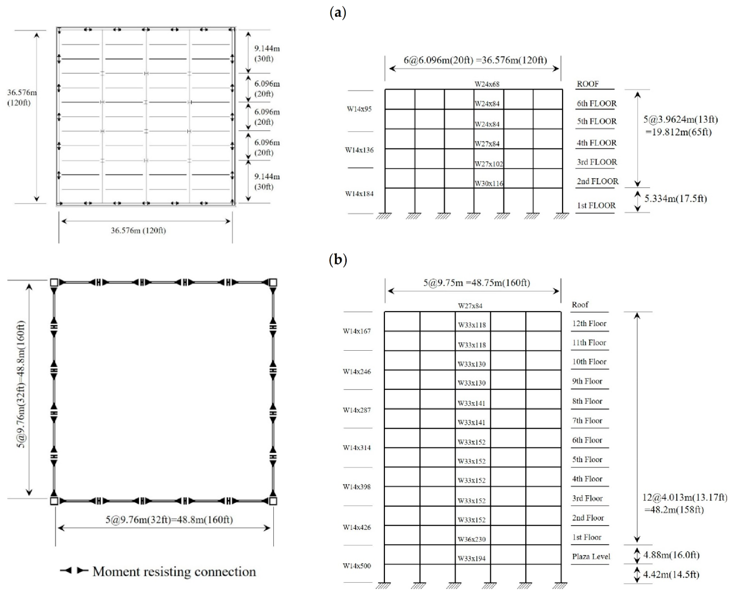
For the maximum displacement estimation and development of fragility curve, we used two types of steel moment-frame buildings with six floors and 13 floors. The six-floor building was designed with the 1973 Uniform Building Code (UBC) requirements in 1976 [34,39]. The building is characterized by a rectangular plan of 36.6 × 36.6 m with 25.3 m in height, and an 8.2 centimeter thick concrete slab. Features of sections are estimated using A-36 steel and the yield stress of 303 MP. The weight of the structure is approximately 34,644 kN. The plan view and member types for the six-floor building is shown in Figure 3a. Detailed descriptions of the target building were presented by Kunnath et al. [40] and Kalkan and Kunnath [41].
The thirteen-story structure is considered as a second illustrative example in this study. It is composed of a basement and 13 floors above the ground. This structure was built in 1975 and designed according to the 1973 UBC requirements. The floor plan of the structure is shown in Figure 3b with elevation view. The building has a rectangular plan of 48.8 × 48.8 m. The exterior frames are moment-resisting frames, and the interior frames are for load bearing. It has been instrumented as part of the Strong Motion Instrumentation Program for six-floor and 13-floor buildings [41,42,43]. Additionally, Song et al. [44] examined ground motion intensity measures and component seismic demand parameters to conduct a probabilistic seismic demand analysis of bridges. In the study, we used the Opensees to carry out the nonlinear dynamic analysis and perform the Newmark beta method for structural analysis. This study focused on developing a structural response estimation model. Detailed structural analysis, including the implementation of a nonlinear time history analysis, the type of method used, nonlinear material parameters and its model, and the nonstructural components, plays an important role in the structural analysis. However, these aspects are beyond the scope of this study. Therefore, the details of related information are briefly mentioned herein. The data for the analysis are obtained from https://www.quakelogic.net/research (accessed on 1 June 2020).
4. Results
4.1. Six-Floor Building Analysis for Development of the Rapid Prediction Model
In this study, the simulation model of the buildings was developed based on the designed data, and the movement of the real building can be represented by the model by adjusting the parameters. The purpose of the study was to develop the estimation model using the maximum displacement, which does not focus on the accuracy analysis and analysis methods. With this data, we estimated the maximum displacement and developed fragility curve using different sampling sets, including 100, 150, 200, 250, 300, 350, and 400. By changing the sampling sizes, the appropriate sampling size can be identified to provide the best performance with the proposed seismic model. In this section, we focus on the six-floor building to estimate the displacement and the fragility curve. To analyze the performance of the selected seismic features in the process, we obtain results from the models based on six selected properties and 13 (full) properties. The variables applied for the simulation are also transformed to obtain standardization and normality; then, the transformed variables are used in the six-parameter-based model and the 13-parameter-based model. The performance of the model is validated using the statistical indices, such as RMSE, R2, NASH, and BIAS.
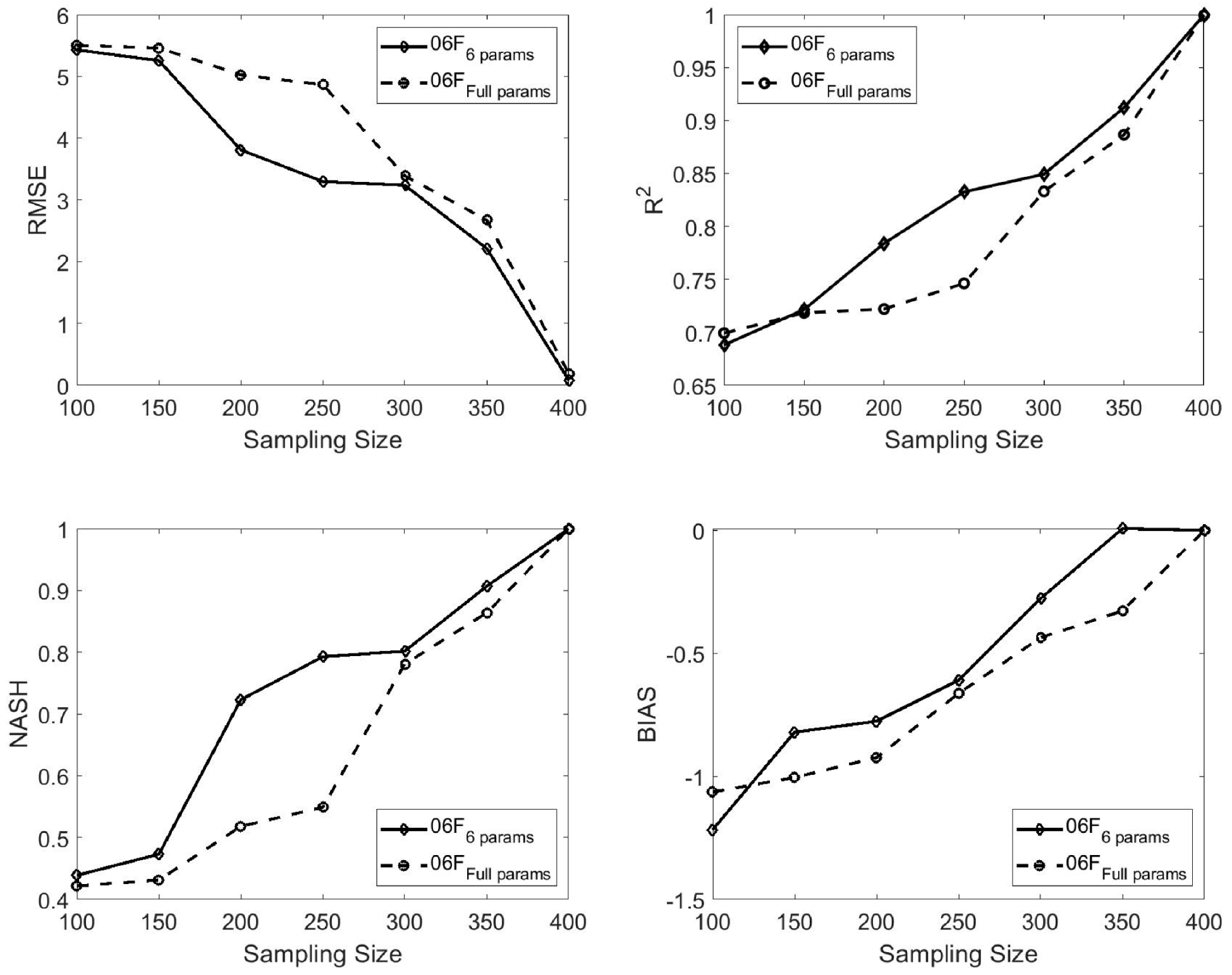
Figure 4 shows the results from various statistical indices for the different sampling size based on the model with six features and 13 features. The six-parameter-based model presents a relatively high performance compared to the 13-parameter-based model. For the RMSE, R2, and NASH, the performance seems to slightly decrease between 150 and 300 sampling sizes with the six features. However, the overall performance appears to be improved when the sampling size increases for the 13 parameter-based model. Based on the observation, we can conclude that the six-parameter-based model for estimating the maximum displacement in seismic analysis tends to provide a satisfactory performance with more accuracy. Table 4 presents the values of the statistical indices for six-parameter-based model and 13-parameter-based model. From the table, we can observe that both models with 400 sampling size produce the best performance, while a sampling size of 100 in both models generates the worst performance.
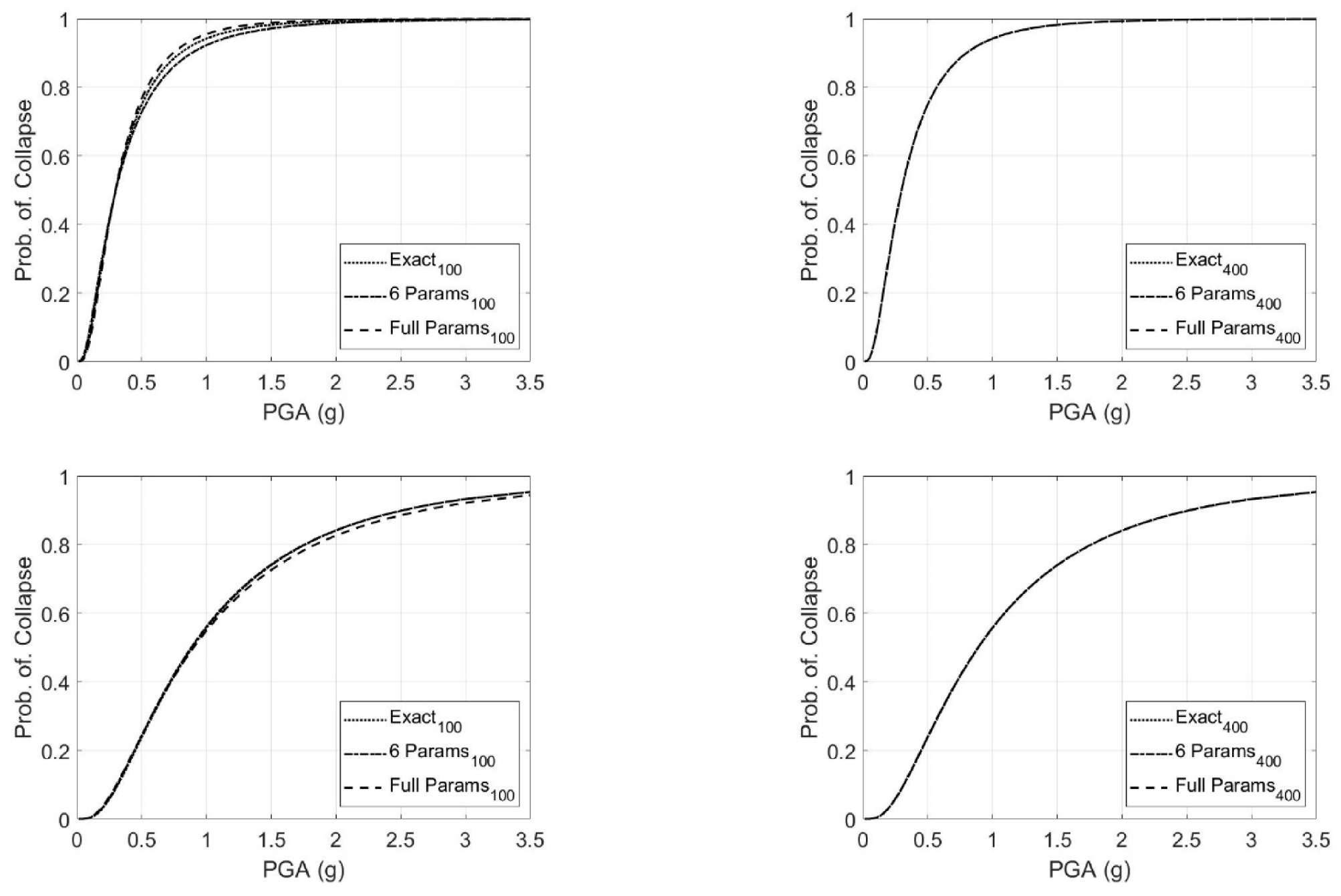
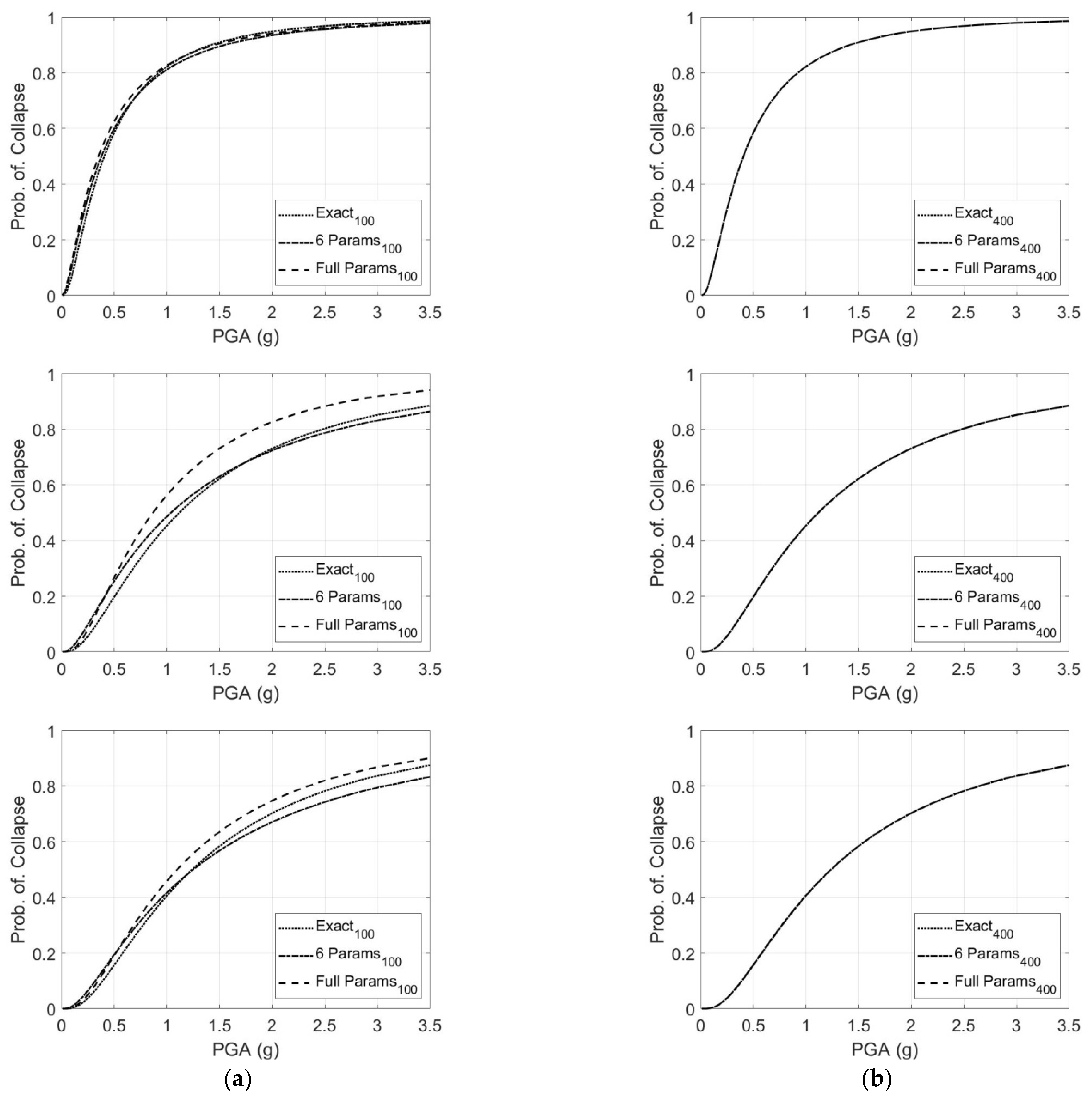
In addition, we developed the seismic fragility curve derived from the maximum displacement for the six-parameter-based model and the 13-parameter-based model. Fragility curves based on IO, LS, and CP levels are shown in Figure 4 by comparing their performance. In the work, we used the MIDR as a performance criterion, while the fragility curve is calculated based on the two data sets (the exact data from simulation and estimation data from the proposed model) with the seismic waves. The levels for IO, LS, and CP determine the acceptance range of MIDR using the maximum height. The performance levels have threshold values considering the IO (0.7%), LS (2.5%), and CP (5.0%) to provide the MIDR limits [27,28,45,46]. Generally, the structural analysis that produces the fragility curve is conducted based on the PGA of 0.0 g in the fragility function. For the analysis, we used the three performance levels (IO, LS, and CP); among the three levels, the CP indicates the entire destruction that we want to obtain by increasing the PGA to 3.5 g. The fragility curve is then estimated based on the log-normal distribution. In other words, the CP requires the point of the entire collapse of the target structures. Therefore, the simulations (e.g., nonlinear dynamic time history analysis) are conducted by increasing the PGA until the structure is collapsed. In the study, the PGA of 3.5 g is selected for the upper limits of the PGA range for the simulation. Figure 5 also presents the results for the model with 100 sampling size and the model with 400 sampling size. A maximum inter-story drift ratio is used for the performance criterion, and the exact data based on results of simulation and the estimated data based on the proposed model are examined for the seismic wave. Most of the figures appear to be the S-curve shape, and the result of the level based on IO tends to show the best performance among different levels. Moreover, the values of the fragility curve function based on the IO level for 100 sampling size show the exact data of −1.2173 and 0.7735, the six-feature data of −1.2103 and 0.8494, and the 13-feature data of −1.2213 and 0.7192 for the median and standard deviation statistics. On the other hand, the values for 400 sampling size present the exact data of −1.2173 and 0.7735, the six-feature data of −1.2170 and 0.7735, and the 13-feature data of −1.2177 and 0.7741 for the median and standard deviation statistics, respectively.
4.2. Thirteen Floor Building Analysis for Development of the Rapid Prediction Model
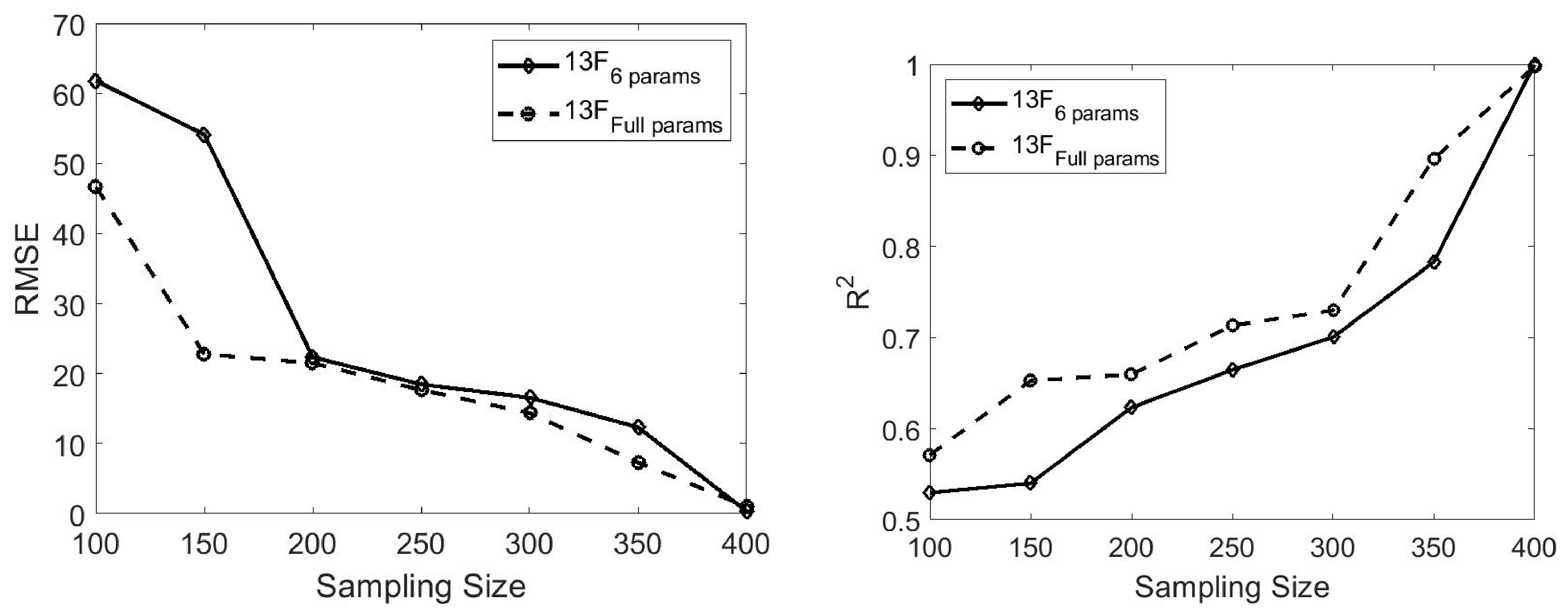
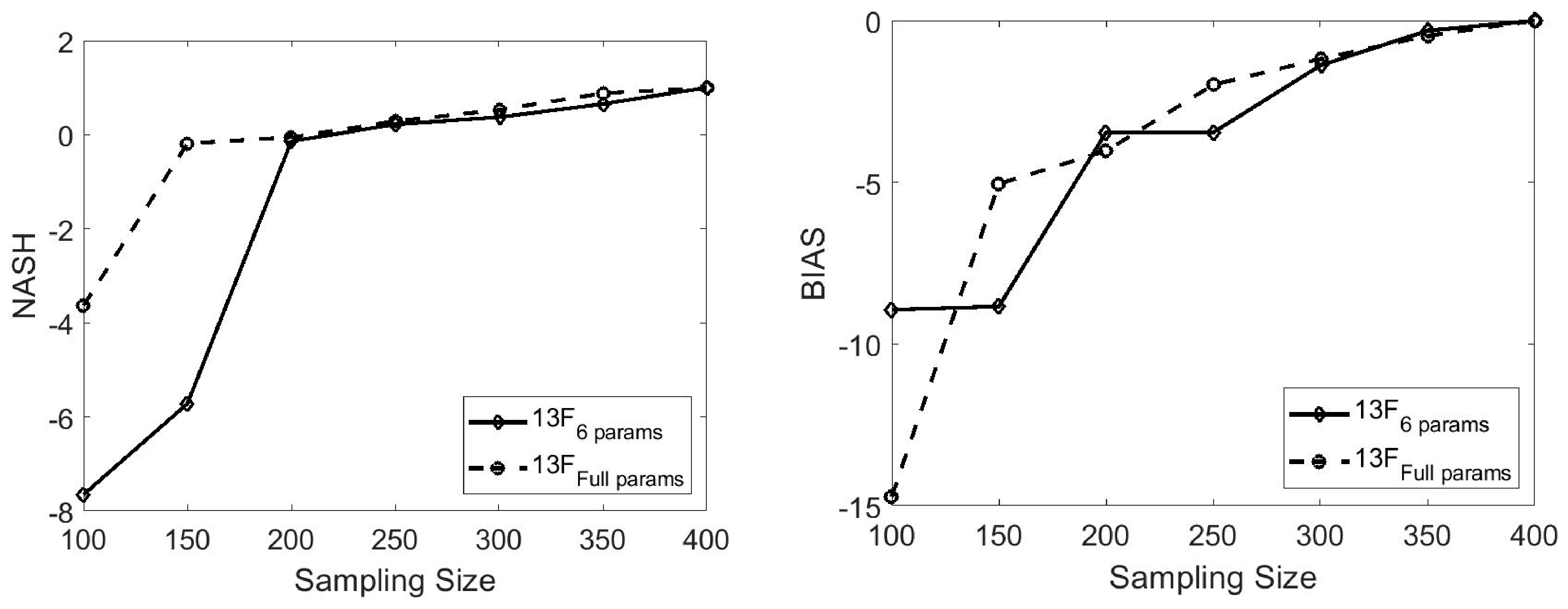
The GPR model is also examined for the 13-floor building, which has more degrees of freedom than the six-floor building. The six-parameter-based and 13-parameter-based models are used to produce the maximum displacement with fragility curve. To assess the model performance, four statistical indices are applied for the results obtained from the seismic model. Figure 6 shows the statistical results using RMSE, R2, NASH, and BIAS, and they show a better estimation as the sampling sizes increase from 100 to 400. As shown in the figure, the model with six features seems to have similar results to the model with 13 features. Furthermore, we can identify that model performance tends to be largely enhanced with the model based on 150 sampling size for the six and 13 features. These results conclude that the six-parameter-based model would be sufficient for estimating the displacement of the 13-floor structure in the seismic analysis. Table 5 presents the values of the indices for both models with various sampling sizes. Among the different sizes, 400 sampling size shows the best performance with the proposed models.
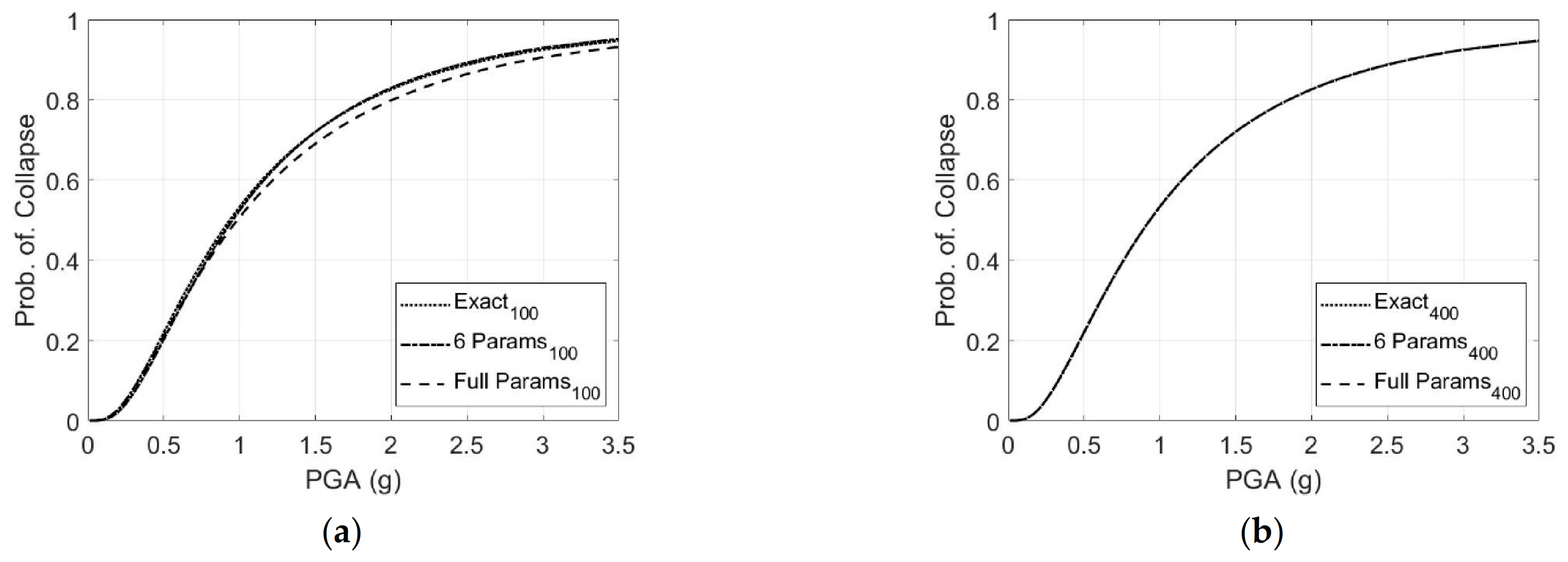
The analysis for the fragility curve is carried out for the 13-floor building based on the IO, LS, and CP levels with the exact data and the estimated data, as performed in the model for the six-floor building. Figure 7 represents the curves for the different levels and different data sampling sizes, including 100 and 400. The curves appear to be the S-curve, and the model with the IO level seems to produce the best performance, compared to the LS and CP levels. The values of the fragility curve function using the IO level with 100 sampling size have the exact data of −0.9051 and 0.9779, the six-feature data of −0.9735 and 1.1005, and the 13-feature data of −1.0502 and 1.1109 for the median and standard deviation statistics, respectively. The values for 400 sampling size have the exact data of −0.9051 and 0.9779, the six-feature data of −0.9045 and 0.9774, and the 13-feature data of −0.9062 and 0.9791 for the median and standard deviation statistics, respectively.
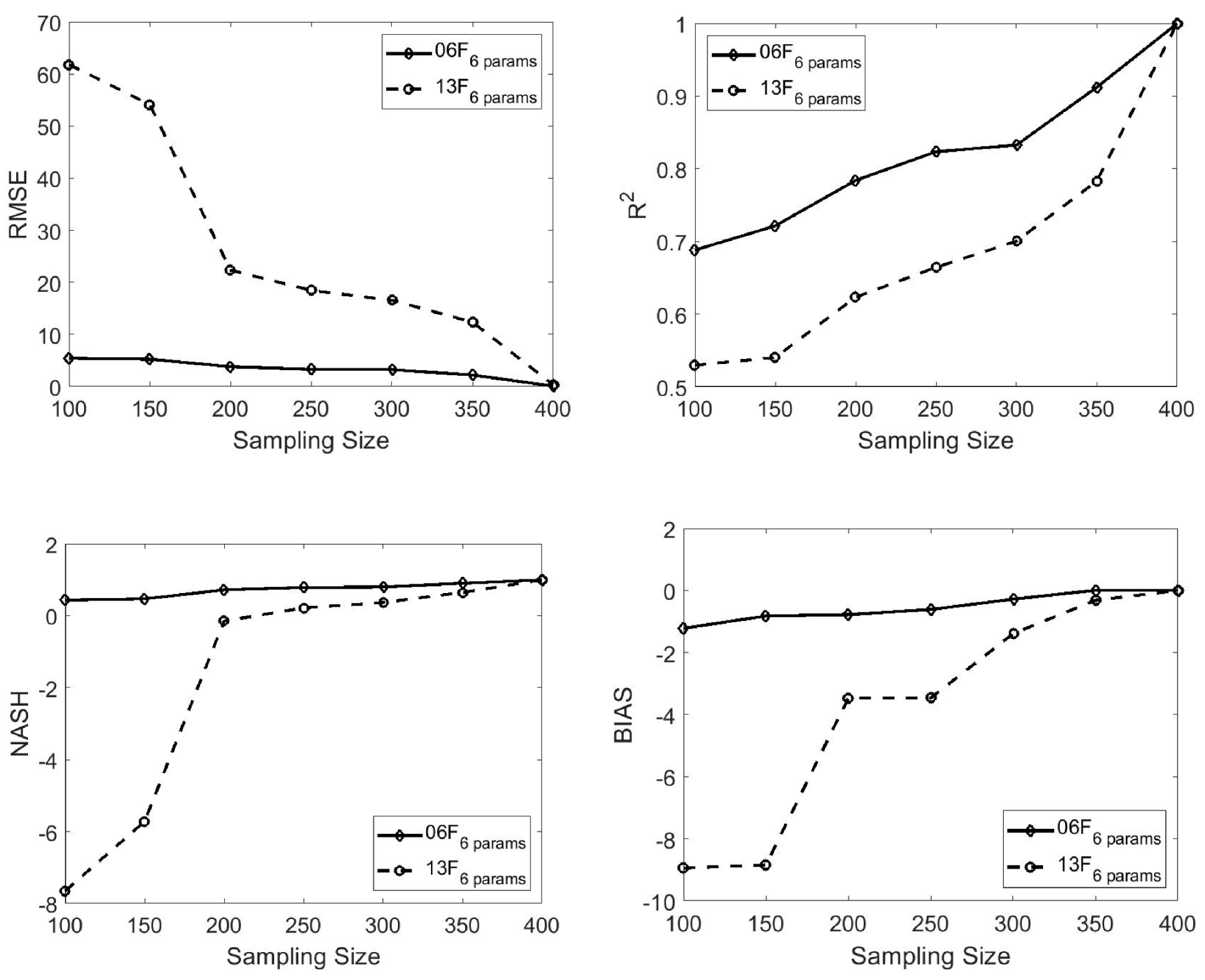
Based on the model with six features, we compare the performance of the six-floor structure to the 13-floor structure in estimating the maximum displacement to identify their trend and the appropriate sampling size. The results for the RMSE, R2, NASH, and BIAS based on the two types of buildings are presented in Figure 8 for different sampling sizes, ranging from 100 to 400. For the six-floor structure, the model performance improves gradually with increasing sampling sizes from the four statistical indices. In estimating the displacement of the six-floor structure, represented as the low height building, a smaller sampling size tends to be sufficient. On the other hand, for the 13-floor structure, we can clearly determine that the model performance largely increases from 100 to 200 sampling size based on the RMSE, NASH, and BIAS. The value of R2 significantly increases from 250 to 350 sampling sizes. This behavior shows that the 13-floor structure, representing a high height building, requires a large sampling size of more than 200. This result is expected because a structure with more complexity (e.g., the 13-floor structure) has more degrees of freedom, which can affect the model performance compared to a lower structure. Table 6 shows the values of the statistical indices for the six-floor and 13-floor structures with various sampling sizes.
5. Discussion with Regional Seismic Damage Assessment
We investigated the structural response (i.e., the maximum displacement) and then performed a seismic vulnerability assessment at Gyeongju by applying the proposed prediction model. The GIS analysis and estimation of structural response were performed. There is a lack of information, such as a prediction model of other structures. However, the proposed approach can be applied to different structural types, and the omitted information can be easily obtained. The US building data can be used as training to conduct the seismic analysis in Gyeongju, because it is based on the results from the simulation model.
5.1. GIS Analysis
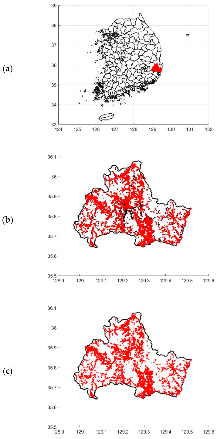
The regional seismic damage assessment is performed using the data set provided by Korea National Spatial Data Infrastructure Portal (http://www.nsdi.go.kr/, accessed on 1 July 2021). Based on the GIS data derived from National Hub Open Data, we combine topographical information of geo-spatial information with GIS integrated building information. Then, the topographical information and the integrated/combined building information are extracted for the analysis of the target region, Gyeongju. The estimation model is developed, in the present study, based on a steel-frame structure, and it is expected to achieve structural responses with maximum displacement for the structures in the area. Among various types of structures in Gyeongju, the steel-frame structure occupies 26.52%. Other structures, such as masonry-frame, concrete-frame, and wood-frame structures, occupy 29.64, 19.53, and 24.19%, respectively. Figure 9 shows the locations of all types of structures in Gyeongju and the locations of the steel-frame structure used for the analysis.
5.2. Estimation of Structural Responses
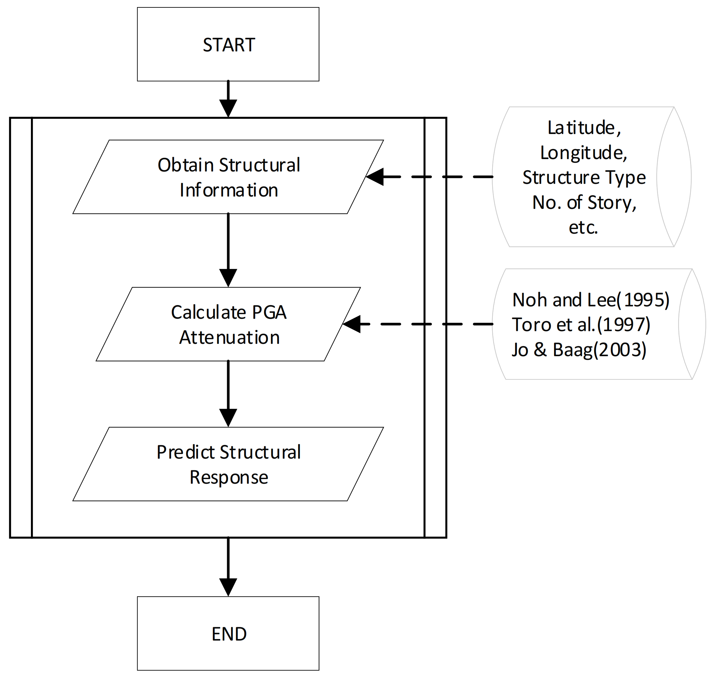
To estimate the structural response, we use the seismic information based on the earthquake at Gyeongju in 2016. The reduction in magnitude for seismic activities is conducted to consider the location of earthquakes and individual buildings in the study region [47]. The reduction equations considered for the analysis follow the equations of Noh and Lee [48], Toro et al. [49], and Jo and Baag [50]. Each equation is applied considering the weight based on 20, 40, and 40%, respectively, to solve uncertainly problems. The entire process for the structural response estimation is shown in Figure 10.
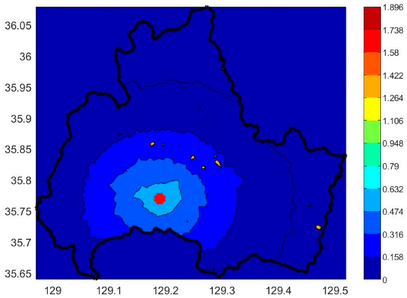
Based on the presented procedure, we estimate the damages from the seismic waves at Gyeongju with the GPR model. From the national and architectural seismic design standard, Gyeongju characterizes the seismic district I, the seismic district coefficient of 0.11 with the return period of 500, and the traditional design standard for earthquake of 0.147 g. The result of the maximum displacement estimation based on the traditional standard is shown in Figure 11 for the steel-frame structures in Gyeongju. Note that there are 32 buildings with more than six floors and 19,984 buildings with fewer than six floors in a total number of 20,016 buildings at the study area.
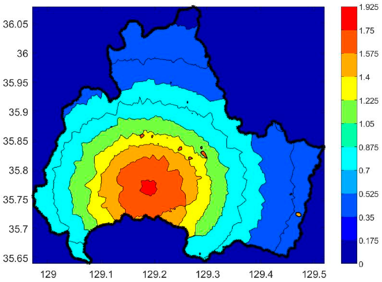
The maximum PGA derived from the occurrence of the Gyeongju earthquake in 2016 is 0.404 g. In this study, the maximum displacement estimated using this maximum PGA is obtained, and the result is presented in Figure 12. From this figure, we can identify that the displacement from the earthquake provides information on the magnitude of the damages occurred due to natural disasters. As a result, the proposed model can be used to generate accurate and rapid responses based on the regional seismic damage assessment utilizing the maximum displacement estimation. In this study, we developed two estimation models, and we applied these models to structures in Gyeongju. The results demonstrate the effectiveness of the proposed models pertaining to vulnerability assessment, and they can be used to developing estimated models in future studies. Additionally, the HAZUS and other tools can be applied for vulnerability assessment after further developing the estimation models.
6. Conclusions
The machine learning framework for the estimation of the maximum displacement and fragility curve is presented in this paper. The GPR model was applied to two types of buildings, i.e., six-floor and 13-floor structures. Additionally, 13 seismic wave features were considered to establish the model, and six features were selected from the correlation analysis using the Pearson correlation coefficient. The six-parameter-based model and 13-parameter-based model were compared to assess the model performance in estimating the maximum displacement. The performance was validated using the RMSE, R2, NASH, and BIAS with 10-fold cross validation, and sensitivity analyses with various sampling sizes of 100, 150, 200, 250, 300, 350, and 400 were performed to determine the proper sampling number for the two structure types.
In the analysis of the models with different numbers of features, the six-parameter-based model presented a similar performance to that of a 13-parameter-based model for both types of the buildings, based on the four statistical indices. The six-parameter-based model seems to provide an acceptable performance in estimating the seismic maximum displacement by reducing the computing cost for the development of estimation models. In the sensitivity analysis of the six-floor building, the model performance improves steadily with the increase in the sampling size. For the 13-floor building, the performance significantly increases for sampling sizes greater than 200. A short building tends to require a smaller sampling size, whereas a tall building tends to require a large sampling size. This might be because a high height structure has more degrees of freedom, which can affect the sampling size.
Furthermore, we examined the development of seismic response models to rapidly estimate seismic damages based on the fragility curve and regional damage assessment. The seismic fragility curve was examined based on the three performance levels, namely, IO, LS, and CP in MIDR. We compared the fragility curves derived from the actual data and estimated data and verified the accuracy of the estimated curve. Regional seismic damage assessment was also investigated by determining the structural response with the maximum displacement. The GPR model based on seismic information on Gyeongju earthquake estimated the maximum displacement considering the maximum PGA of 0.404 g. The result apparently indicates that the estimation of structural response can establish advanced seismic models with the displacement estimation and can assist in political decisions by providing robust and prompt responses from seismic activities. The maximum structural displacement, playing an important role in seismic risk assessment, can be quickly and accurately estimated using the proposed models based on seismic activities and then easily applied for constructing fragility curves by providing a probabilistic damage information and regional seismic damage prediction. Potentially, the estimated structural damage information can be helpful for decision-makers, city planners, etc. Future work should focus on various structural types by applying for the GPR or other techniques to obtain an accurate estimation of the maximum seismic displacement.
Author Contributions
Conceptualization, Sangki Park and Kichul Jung; methodology, Sangki Park and Kichul Jung; investigation, Sangki Park; funding acquisition, Sangki Park and Kichul Jung; writing, review, and editing, Sangki Park and Kichul Jung. All authors have read and agreed to the published version of the manuscript.
Funding
This research was supported by the Basic Science Research Program of the National Research Foundation of Korea (NRF), funded by the Ministry of Education (Grant 2019R1I1A1A01061109), and by the Korea Agency for Infrastructure Technology Advancement (KAIA) grant funded by the Ministry of Land, Infrastructure and Transport (Grant 21RMPP-C163162-01).
Institutional Review Board Statement
Not applicable.
Informed Consent Statement
Not applicable.
Data Availability Statement
Not applicable.
Acknowledgments
The authors would like to acknowledge support given by the NRF and KAIA.
Conflicts of Interest
The authors declare no conflict of interest.
References
- Cimellaro, G.P.; Reinhorn, A.M.; Bruneau, M. Performance-based metamodel for healthcare facilities. Earthq. Eng. Struct. Dyn. 2011, 40, 1197–1217. [Google Scholar] [CrossRef]
- Wang, Z.; Pedroni, N.; Zentner, I.; Zio, E. Seismic fragility analysis with artificial neural networks: Application to nuclear power plant equipment. Eng. Struct. 2018, 162, 213–225. [Google Scholar] [CrossRef] [Green Version]
- Porter, K.A.; Kiremidjian, A.S.; LeGrue, J.S. Assembly-based vulnerability of buildings and its use in performance evaluation. Earthq. Spectra 2001, 17, 291–312. [Google Scholar] [CrossRef]
- Iervolino, I.; Giorgio, M. Stochastic modeling of recovery from seismic shocks. In Proceedings of the 12th International Conference on Applications of Statistics and Probability in Civil Engineering, Vancouver, BC, Canada, 12–15 July 2015. [Google Scholar]
- Burton, H.V.; Deierlein, G.; Lallemant, D.; Lin, T. Framework for incorporating probabilistic building performance in the assessment of community seismic resilience. J. Struct. Eng. 2016, 142, C4015007. [Google Scholar] [CrossRef] [Green Version]
- Shinozuka, M.; Feng, M.Q.; Lee, J.; Naganuma, T. Statistical analysis of fragility curves. J. Eng. Mech. 2000, 126, 1224–1231. [Google Scholar] [CrossRef] [Green Version]
- Shinozuka, M.; Feng, M.Q.; Kim, H.-K.; Kim, S.-H. Nonlinear static procedure for fragility curve development. J. Eng. Mech. 2000, 126, 1287–1295. [Google Scholar] [CrossRef] [Green Version]
- Reed, J.W.; Kennedy, R.P. Methodology for Developing Seismic Fragilities; Final Report TR-103959; Electric Power Research Institute: Palo Alto, CA, USA, 1994. [Google Scholar]
- Kirçil, M.S.; Polat, Z. Fragility analysis of mid-rise R/C frame buildings. Eng. Struct. 2006, 28, 1335–1345. [Google Scholar] [CrossRef]
- Araya-Letelier, G.; Parra, P.; Lopez-Garcia, D.; Garcia-Valdes, A.; Candia, G.; Lagos, R. Collapse risk assessment of a Chilean dual wall-frame reinforced concrete office building. Eng. Struct. 2019, 183, 770–779. [Google Scholar]
- Shafei, B.; Zareian, F.; Lignos, D.G. A simplified method for collapse capacity assessment of moment-resisting frame and shear wall structural systems. Eng. Struct. 2011, 33, 1107–1116. [Google Scholar] [CrossRef]
- Ferreira, T.M.; Estêvão, J.; Maio, R.; Vicente, R. The use of Artificial Neural Networks to estimate seismic damage and derive vulnerability functions for traditional masonry. Front. Struct. Civ. Eng. 2020, 14, 609–622. [Google Scholar] [CrossRef]
- Yariyan, P.; Zabihi, H.; Wolf, I.D.; Karami, M.; Amiriyan, S. Earthquake risk assessment using an integrated Fuzzy Analytic Hierarchy Process with Artificial Neural Networks based on GIS: A case study of Sanandaj in Iran. Int. J. Disaster Risk Reduct. 2020, 50, 101705. [Google Scholar] [CrossRef]
- Hwang, S.H.; Mangalathu, S.; Shin, J.; Jeon, J.S. Machine learning-based approaches for seismic demand and collapse of ductile reinforced concrete building frames. J. Build. Eng. 2021, 34, 101905. [Google Scholar] [CrossRef]
- Lagaros, N.D.; Fragiadakis, M. Fragility assessment of steel frames using neural networks. Earthq. Spectra 2007, 23, 735–752. [Google Scholar] [CrossRef]
- Unnikrishnan, V.; Prasad, A.; Rao, B. Development of fragility curves using high-dimensional model representation. Earthq. Eng. Struct. Dyn. 2013, 42, 419–430. [Google Scholar] [CrossRef]
- Saha, S.K.; Matsagar, V.; Chakraborty, S. Uncertainty quantification and seismic fragility of base-isolated liquid storage tanks using response surface models. Probabilistic Eng. Mech. 2016, 43, 20–35. [Google Scholar] [CrossRef]
- Calabrese, A.; Lai, C.G. Fragility functions of blockwork wharves using artificial neural networks. Soil Dyn. Earthq. Eng. 2013, 52, 88–102. [Google Scholar] [CrossRef]
- Gehl, P.; D’Ayala, D. Development of Bayesian Networks for the multi-hazard fragility assessment of bridge systems. Struct. Saf. 2016, 60, 37–46. [Google Scholar] [CrossRef]
- Jung, K.; Park, D.; Park, S. Development of Models for Prompt Responses from Natural Disasters. Sustainability 2020, 12, 7803. [Google Scholar] [CrossRef]
- Cummings, D.; Dalrymple, R.; Choi, K.; Jin, J. The Tide-Dominated Han River Delta, Korea: Geomorphology, Sedimentology, and Stratigraphic Architecture; Elsevier: Amsterdam, The Netherlands, 2015. [Google Scholar]
- Han, J.; Kim, J.; Park, S.; Son, S.; Ryu, M. Seismic Vulnerability Assessment and Mapping of Gyeongju, South Korea Using Frequency Ratio, Decision Tree, and Random Forest. Sustainability 2020, 12, 7787. [Google Scholar] [CrossRef]
- Park, B.K.; Kim, S.W. Recent tectonism in the Korean Peninsula and sea floor spreading. Econ. Environ. Geol. 1971, 4, 39–43. [Google Scholar]
- Park, S.C.; Yang, H.; Lee, D.K.; Park, E.H.; Lee, W.-J. Did the 12 September 2016 Gyeongju, South Korea earthquake cause surface deformation? Geosci. J. 2018, 22, 337–346. [Google Scholar] [CrossRef]
- Schulz, E.; Speekenbrink, M.; Krause, A. A tutorial on Gaussian process regression: Modelling, exploring, and exploiting functions. J. Math. Psychol. 2018, 85, 1–16. [Google Scholar] [CrossRef]
- Chalupka, K.; Williams Iain Murray, C.K.I. A framework for evaluating approximation methods for Gaussian progress regression. J. Mach. Learn. Res. 2013, 14, 333–350. [Google Scholar]
- Phan, H.N.; Paolacci, F.; Di Filippo, R.D.; Bursi, O.S. Seismic vulnerability of above-ground storage tanks with unanchored support conditions for Na-tech risks based on Gaussian process regression. Bull. Earthq. Eng. 2020, 18, 6883–6906. [Google Scholar] [CrossRef]
- Hoang, P.H.; Phan, H.N.; Nguyen, D.T.; Paolacci, F. Kriging Metamodel-Based Seismic Fragility Analysis of Single-Bent Reinforced Concrete Highway Bridges. Buildings 2021, 11, 238. [Google Scholar] [CrossRef]
- Williams, C.K.; Rasmussen, C.E. Gaussian Processes for Machine Learning; MIT Press: Cambridge, MA, USA, 2006. [Google Scholar]
- Nakamura, T.; TN, T.S.; Shinozuka, M. A study on failure probability of highway bridges by earthquake based on statistical method. In Proceedings of the 10th Japanese Earthquake Engineering Symposium, Minato City, Tokyo, Japan, 25–27 November 1998. [Google Scholar]
- Miller, R.G. A trustworthy jackknife. Ann. Math. Stat. 1964, 35, 1594–1605. [Google Scholar] [CrossRef]
- Shao, J.; Tu, D. The Jackknife and Bootstrap; Springer: Berlin, Germany, 2012. [Google Scholar]
- Shu, C.; Ouarda, T.B.M.J. Flood frequency analysis at ungauged sites using artificial neural networks in canonical correlation analysis physiographic space. Water Resour. Res. 2007, 43. [Google Scholar] [CrossRef] [Green Version]
- Basilevsky, A.T. Statistical Factor Analysis and Related Methods: Theory and Applications; John Wiley & Sons Inc.: London, UK, 2009. [Google Scholar]
- Singh, G.; Panda, R.K. Daily sediment yield modelling with artificial neural network using 10-fold cross validation method: A small agricultural watershed, Kapgari, India. Int. J. Earth Sci. Eng. 2011, 4, 443–450. [Google Scholar]
- Rodriguez, J.D.; Perez, A.; Lozano, J.A. Sensitivity analysis of k-fold cross validation in prediction error estimation. IEEE Trans. Pattern Anal. Mach. Intell. 2010, 32, 569–575. [Google Scholar] [CrossRef]
- Jung, K.; Ouarda, T.B.M.J.; Marpu, P.R. On the value of river network information in regional frequency analysis. J. Hydrometeorol. 2021, 22, 201–216. [Google Scholar] [CrossRef]
- Rahman, A.; Charron, C.; Ouarda, T.B.M.J.; Chebana, F. Development of regional flood frequency analysis techniques using generalized additive models for Australia. Stoch. Environ. Res. Risk Assess. 2018, 32, 123–139. [Google Scholar] [CrossRef]
- Papazafeiropoulos, G.; Plevris, V. OpenSeismoMatlab: A new open-source software for strong ground motion data processing. Heliyon 2018, 4, e00784. [Google Scholar] [CrossRef] [PubMed] [Green Version]
- Kunnath, S.K.; Nghiem, Q.; El-Tawil, S. Modeling and response prediction in performance-based seismic evaluation: Case studies of instrumented steel moment-frame buildings. Earthq. Spectra 2004, 20, 883–915. [Google Scholar] [CrossRef]
- Kalkan, E.; Kunnath, S.K. Effects of fling step and forward directivity on seismic response of buildings. Earthq. Spectra 2006, 22, 367–390. [Google Scholar] [CrossRef]
- Kalkan, E.; Chopra, A.K. Practical guidelines to select and scale earthquake records for nonlinear response history analysis of structures. US Geol. Surv. Open-File Rep. 2010, 1068, 126. [Google Scholar]
- Uang, C.-M. Performance of a 13-Story Steel Moment-Resisting Frame Damaged in the 1994 Northridge Earthquake; Structural Systems Research; University of California: San Diego, CA, USA, 1995. [Google Scholar]
- Song, S.; Qian, C.; Qian, Y.; Bao, H.; Lin, P. Canonical Correlation Analysis of Selecting Optimal Ground Motion Intensity Measures for Bridges. KSCE J. Civ. Eng. 2019, 23, 2958–2970. [Google Scholar] [CrossRef]
- ASCE/SEI 41-06. Seismic Rehabilitation of Existing Buildings; Ameriacan Society of Civil Engineers: Reston, VA, USA, 2007. [Google Scholar]
- Rezaei, S.; Akbari Hamed, A.; Basim, M.C. Seismic performance evaluation of steel structures equipped with dissipative columns. J. Build. Eng. 2020, 29, 101227. [Google Scholar] [CrossRef]
- Kim, M.-J.; Kyung, J.-B. An analysis of the sensitivity of input parameters for the seismic hazard analysis in the Korean Peninsula. J. Korean Earth Sci. Soc. 2015, 36, 351–359. [Google Scholar] [CrossRef]
- Noh, M.H.; Lee, K.H. Estimation of Peak Ground Motions in the Southeastern Part of the Korean peninsula (II): Development of Predictive Equations. J. Geol. Soc. Korea 1995, 31, 175–187. [Google Scholar]
- Toro, G.R.; Abrahamson, N.A.; Schneider, J.F. Model of strong ground motions from earthquakes in central and eastern North America: Best estimates and uncertainties. Seismol. Res. Lett. 1997, 68, 41–57. [Google Scholar] [CrossRef]
- Jo, N.; Baag, C. Estimation of spectrum decay parameter k and stochastic prediction of strong ground motions in southeastern Korea. J. Earthq. Eng. Soc. Korea 2003, 7, 59–70. [Google Scholar]
Figure 1.
Procedure for obtaining the maximum displacement and fragility curves.

Figure 2.
The 400 Seismic waves with the response spectrum analysis used in the study.

Figure 3.
Structural configuration based on floor plan view and elevation view for the (a) six-floor building and (b) 13-floor building.
Figure 3.
Structural configuration based on floor plan view and elevation view for the (a) six-floor building and (b) 13-floor building.

Figure 4.
Results of the four statistical indices for the maximum displacement estimation using the six-floor building.
Figure 4.
Results of the four statistical indices for the maximum displacement estimation using the six-floor building.

Figure 5.
Fragility curves using 6-floor structure for (a) 100 sampling size with IO (upper left), LS (center left), and CP (lower left) levels, and (b) 400 sampling size with IO (upper right), LS (center right), and CP (lower right) levels.
Figure 5.
Fragility curves using 6-floor structure for (a) 100 sampling size with IO (upper left), LS (center left), and CP (lower left) levels, and (b) 400 sampling size with IO (upper right), LS (center right), and CP (lower right) levels.


Figure 6.
Results for the four statistical indices including RMSE (upper left), R2 (upper right), NASH (lower left), and BIAS (lower right) for the maximum displacement estimation using 13-floor building.
Figure 6.
Results for the four statistical indices including RMSE (upper left), R2 (upper right), NASH (lower left), and BIAS (lower right) for the maximum displacement estimation using 13-floor building.


Figure 7.
Fragility curves using 13-floor structure for (a) 100 sampling size with IO (upper left), LS (center left), and CP (lower left) levels; and (b) 400 sampling size with IO (upper right), LS (center right), and CP (lower right) levels.
Figure 7.
Fragility curves using 13-floor structure for (a) 100 sampling size with IO (upper left), LS (center left), and CP (lower left) levels; and (b) 400 sampling size with IO (upper right), LS (center right), and CP (lower right) levels.

Figure 8.
Results for the four statistical indices including RMSE (upper left), R2 (upper right), NASH (lower left), and BIAS (lower right) for the maximum displacement estimation using six-floor and 13-floor buildings.
Figure 8.
Results for the four statistical indices including RMSE (upper left), R2 (upper right), NASH (lower left), and BIAS (lower right) for the maximum displacement estimation using six-floor and 13-floor buildings.

Figure 9.
Study maps for (a) Gyeongju in South Korea, (b) locations of all types of structures in Gyeongju, (c) locations of the steel-frame structure in Gyeongju.
Figure 9.
Study maps for (a) Gyeongju in South Korea, (b) locations of all types of structures in Gyeongju, (c) locations of the steel-frame structure in Gyeongju.

Figure 10.
Process for the prediction of the structural response considering the reduction in magnitude for seismic activities.
Figure 10.
Process for the prediction of the structural response considering the reduction in magnitude for seismic activities.

Figure 11.
Map for the maximum displacement estimation based on the traditional design standard for earthquake of 0.147 g in Gyeongju.
Figure 11.
Map for the maximum displacement estimation based on the traditional design standard for earthquake of 0.147 g in Gyeongju.

Figure 12.
Map for the maximum displacement estimation based on the maximum PGA of 0.404 g with Gyeongju earthquake in Gyeongju.
Figure 12.
Map for the maximum displacement estimation based on the maximum PGA of 0.404 g with Gyeongju earthquake in Gyeongju.


Table 1.
The 13 seismic wave features with the statistical analysis.
| Name | Min | Max | Average |
|---|---|---|---|
| Arias Intensity (m/s2) | 5.584 × 10⁻¹² | 1.903 | 0.104 |
| CAV (g.sec) | 0.017 | 16.428 | 3.264 |
| Characteristic Intensity (m/s2) | 3.550 × 10⁻⁹ | 2.545 | 0.234 |
| Abs Min/Max difference of PGA | 0.00083 | 3.029 | 0.309 |
| Cumulative Energy | 5.744 × 10⁻⁵ | 12.913 | 1.142 |
| Mean Frequency (Hz) | 0.668 | 9.710 | 3.666 |
| PGA (g) | 0.020 | 3.500 | 0.894 |
| PGV (m/s) | 1.724 × 10⁻⁶ | 0.005 | 0.00061 |
| PGD (m) | 7.340 × 10⁻¹⁰ | 5.825 × 10⁻⁵ | 3.341 × 10⁻⁶ |
| PVA ratio | 8.620 × 10⁻⁵ | 0.007 | 0.00087 |
| Total Duration (sec) | 3.560 | 147.590 | 19.353 |
| Significant duration (sec) | 3.570 | 147.595 | 19.361 |
| Mean period (Hz) | 0.165 | 2.076 | 0.557 |
Table 2.
Seismic wave features used in the study.
| ID | Feature Name |
|---|---|
| 1 | Arias intensity |
| 2 | CAV |
| 3 | Characteristic intensity |
| 4 | Difference between min and max |
| 5 | ECUM |
| 6 | FM |
| 7 | PGA |
| 8 | PGV |
| 9 | PGD |
| 10 | PVA ratio |
| 11 | Duration (5% and 95%) |
| 12 | Td |
| 13 | Tm |
Table 3.
Correlation analysis for the characteristics based on Pearson coefficients.
| ID1 | ID2 | ID3 | ID4 | ID5 | ID6 | ID7 | ID8 | ID9 | ID10 | ID11 | ID12 | ID13 | Use | |
| ID1 | 1.00 | 0.76 | 0.97 | 0.48 | 0.86 | 0.20 | 0.70 | 0.47 | 0.28 | 0.15 | 0.03 | 0.03 | 0.28 | O |
| ID2 | 1.00 | 0.75 | 0.56 | 0.89 | 0.25 | 0.78 | 0.59 | 0.40 | 0.11 | 0.17 | 0.17 | 0.27 | O | |
| ID3 | 1.00 | 0.53 | 0.84 | 0.23 | 0.75 | 0.51 | 0.30 | 0.17 | 0.07 | 0.07 | 0.31 | × | ||
| ID4 | 1.00 | 0.62 | 0.50 | 0.76 | 0.73 | 0.49 | 0.05 | 0.19 | 0.19 | 0.41 | × | |||
| ID5 | 1.00 | 0.29 | 0.83 | 0.57 | 0.37 | 0.17 | 0.06 | 0.06 | 0.35 | O | ||||
| ID6 | 1.00 | 0.47 | 0.14 | 0.09 | 0.35 | 0.29 | 0.29 | 0.66 | O | |||||
| ID7 | 1.00 | 0.59 | 0.28 | 0.28 | 0.21 | 0.21 | 0.46 | O | ||||||
| ID8 | 1.00 | 0.83 | 0.35 | 0.06 | 0.06 | 0.14 | ▲ | |||||||
| ID9 | 1.00 | 0.45 | 0.05 | 0.05 | 0.08 | ▲ | ||||||||
| ID10 | 1.00 | 0.30 | 0.30 | 0.56 | × | |||||||||
| ID11 | 1.00 | 0.99 | 0.46 | × | ||||||||||
| ID12 | 1.00 | 0.46 | × | |||||||||||
| ID13 | 1.00 | O |
The bold values indicate the high correlation (more than 0.80). O indicates “use”, × means “not use”, and ▲ implies “not use due to the extra simulation”.
Table 4.
Statistical results for different parameters and various sampling sizes based on the six-floor building.
Table 4.
Statistical results for different parameters and various sampling sizes based on the six-floor building.
| 100 | 150 | 200 | 250 | 300 | 350 | 400 | ||
|---|---|---|---|---|---|---|---|---|
| RMSE | 6 params | 5.4300 | 5.2541 | 3.8081 | 3.2979 | 3.2358 | 2.2118 | 0.0774 |
| 13 params | 5.5045 | 5.4602 | 5.0244 | 4.8633 | 3.3894 | 2.6728 | 0.1866 | |
| R2 | 6 params | 0.6881 | 0.7214 | 0.7839 | 0.8235 | 0.8325 | 0.9121 | 0.9999 |
| 13 params | 0.6991 | 0.7183 | 0.7219 | 0.7461 | 0.8330 | 0.8866 | 0.9999 | |
| NASH | 6 params | 0.4389 | 0.4730 | 0.7232 | 0.7926 | 0.8017 | 0.9067 | 0.9999 |
| 13 params | 0.4216 | 0.4312 | 0.5181 | 0.5490 | 0.7807 | 0.8636 | 0.9993 | |
| BIAS | 6 params | −1.2174 | −0.8205 | −0.7758 | −0.6096 | −0.2774 | 0.0073 | 0.0006 |
| 13 params | −1.0639 | −1.0049 | −0.9237 | −0.6630 | −0.4363 | −0.3272 | 0.0000 |
Table 5.
Statistical results for different parameters and various sampling sizes based on the 13-floor building.
Table 5.
Statistical results for different parameters and various sampling sizes based on the 13-floor building.
| 100 | 150 | 200 | 250 | 300 | 350 | 400 | ||
|---|---|---|---|---|---|---|---|---|
| RMSE | 6 params | 61.7917 | 54.1377 | 22.3553 | 18.4622 | 16.5705 | 12.3378 | 0.3505 |
| 13 params | 46.6716 | 22.7955 | 21.4977 | 17.6729 | 14.3694 | 7.3180 | 1.0307 | |
| R2 | 6 params | 0.5297 | 0.5402 | 0.6232 | 0.6643 | 0.7003 | 0.7828 | 0.9997 |
| 13 params | 0.5711 | 0.6528 | 0.6594 | 0.7131 | 0.7297 | 0.8961 | 0.9976 | |
| NASH | 6 params | −7.6522 | −5.7187 | −0.1437 | 0.2195 | 0.3714 | 0.6520 | 0.9997 |
| 13 params | −3.6343 | −0.1890 | −0.0562 | 0.2852 | 0.5276 | 0.8774 | 0.9976 | |
| BIAS | 6 params | −8.9402 | −8.8389 | −3.4629 | −3.4605 | −1.3888 | −0.3119 | 0.0008 |
| 13 params | −14.7187 | −5.0456 | −4.0346 | −1.9865 | −1.1869 | −0.4691 | −0.0017 |
Table 6.
Statistical results for six parameters and various sampling sizes based on the six-floor and 13-floor buildings.
Table 6.
Statistical results for six parameters and various sampling sizes based on the six-floor and 13-floor buildings.
| 100 | 150 | 200 | 250 | 300 | 350 | 400 | ||
|---|---|---|---|---|---|---|---|---|
| RMSE | 6 floors | 5.4300 | 5.2541 | 3.8081 | 3.2979 | 3.2358 | 2.2118 | 0.0774 |
| 13 floors | 61.7917 | 54.1377 | 22.3553 | 18.4622 | 16.5705 | 12.3378 | 0.3505 | |
| R2 | 6 floors | 0.6881 | 0.7214 | 0.7839 | 0.8235 | 0.8325 | 0.9121 | 0.9999 |
| 13 floors | 0.5297 | 0.5402 | 0.6232 | 0.6643 | 0.7003 | 0.7828 | 0.9997 | |
| NASH | 6 floors | 0.4389 | 0.4730 | 0.7232 | 0.7926 | 0.8017 | 0.9067 | 0.9999 |
| 13 floors | −3.6343 | −0.1890 | −0.0562 | 0.2852 | 0.5276 | 0.8774 | 0.9976 | |
| BIAS | 6 floors | −1.2174 | −0.8205 | −0.7758 | −0.6096 | −0.2774 | 0.0073 | 0.0006 |
| 13 floors | −8.9402 | −8.8389 | −3.4629 | −3.4605 | −1.3888 | −0.3119 | 0.0008 |
Publisher’s Note: MDPI stays neutral with regard to jurisdictional claims in published maps and institutional affiliations. |
© 2021 by the authors. Licensee MDPI, Basel, Switzerland. This article is an open access article distributed under the terms and conditions of the Creative Commons Attribution (CC BY) license (https://creativecommons.org/licenses/by/4.0/).
Share and Cite
MDPI and ACS Style
Park, S.; Jung, K. Gaussian Process Regression-Based Structural Response Model and Its Application to Regional Damage Assessment. ISPRS Int. J. Geo-Inf. 2021, 10, 574. https://0-doi-org.brum.beds.ac.uk/10.3390/ijgi10090574
AMA Style
Park S, Jung K. Gaussian Process Regression-Based Structural Response Model and Its Application to Regional Damage Assessment. ISPRS International Journal of Geo-Information. 2021; 10(9):574. https://0-doi-org.brum.beds.ac.uk/10.3390/ijgi10090574
Chicago/Turabian StylePark, Sangki, and Kichul Jung. 2021. "Gaussian Process Regression-Based Structural Response Model and Its Application to Regional Damage Assessment" ISPRS International Journal of Geo-Information 10, no. 9: 574. https://0-doi-org.brum.beds.ac.uk/10.3390/ijgi10090574
Note that from the first issue of 2016, this journal uses article numbers instead of page numbers. See further details here.