

Parametric Modeling Method for 3D Symbols of Fold Structures

1
Key Laboratory of Virtual Geographic Environment (Nanjing Normal University), Ministry of Education, Nanjing 210023, China
2
Jiangsu Center for Collaborative Innovation in Geographical Information Resource Development and Application, Nanjing 210023, China
3
State Key Laboratory Cultivation Base of Geographical Environment Evolution (Jiangsu Province), Nanjing 210023, China
4
Shandong Rail Transit Engineering Consulting Co., Ltd., Jinan 250101, China
*
Author to whom correspondence should be addressed.
ISPRS Int. J. Geo-Inf. 2022, 11(12), 618; https://0-doi-org.brum.beds.ac.uk/10.3390/ijgi11120618
Submission received: 3 November 2022
/
Revised: 4 December 2022
/
Accepted: 12 December 2022
/
Published: 13 December 2022
(This article belongs to the Special Issue Cartography and Geomedia)
Abstract
:Most fabrication methods for three-dimensional (3D) geological symbols are limited to two types: directly increasing the dimensionality of a 2D geological symbol or performing appropriate modeling for an actual 3D geological situation. The former can express limited vertical information and only applies to the three-dimensional symbol-making of point mineral symbols, while the latter weakens the difference between 3D symbols and 3D geological models and has several disadvantages, such as high dependence on measured data, redundant 3D symbol information, and low efficiency when displayed in a 3D scene. Generating a 3D geological symbol is represented by the process of constructing a 3D geological model. This study proposes a parametric modeling method for 3D fold symbols according to the complexity and diversity of the fold structures. The method involves: (1) obtaining the location of each cross-section in the symbol model, based on the location parameters; (2) constructing the middle cross-section, based on morphological parameters and the Bezier curve; (3) performing affine transformation according to the morphology of the hinge zone and the middle section to generate the sections at both ends of the fold; (4) generating transition sections of the 3D symbol model, based on morphing interpolation; and (5) connecting the point sets of each transition section and stitching them to obtain a 3D fold-symbol model. Case studies for different typical fold structures show that this method can eliminate excessive dependence on geological survey data in the modeling process and realize efficient, intuitive, and abstract 3D symbol modeling of fold structures based on only a few parameters. This method also applies to the 3D geological symbol modeling of faults, joints, intrusions, and other geological structures and 3D geological modeling of typical geological structures with a relatively simple spatial morphology.
1. Introduction
In recent years, traditional geographic information system (GIS) technology and its applications have undergone revolutionary changes [1,2], and it has transformed from 2D GIS to 3D GIS, with a primary focus on 3D modeling, 3D scene display, and 3D spatial analysis [3]. In particular, 3D GIS has become one of the iconic contents of GIS technology today and for the future [4,5]. At present, Digital Earth systems, including Google Earth, NASA WorldWind and Cesium, have been widely embraced by geoscientists in various disciplines. These 3D GIS-related technologies are convenient tools for promoting the scientific research of different application scenarios and contribute to integrating geospatial information, improving visualization capabilities, exploring spatio-temporal changes, and communicating scientific results [6,7,8]. In this context, traditional 2D map symbols cannot easily meet the demand for the intuitive expression of complex geological objects in 3D GIS. The research and application of 3D symbols have gradually become a hot topic in the current GIS field [9,10].
Similar to traditional 2D symbols, 3D symbols are also the language of map visualization, which aims to express the 3D spatial distribution and attribute information of geographical entities [11,12]. The essence of a 3D symbol is that it is a 3D model that directly reflects the spatial morphology of the corresponding geographical object. Therefore, the production of 3D symbols is the process of generating 3D models. Given the growing demand for 3D symbols in 3D GIS applications, such as virtual reality (VR)\augmented reality (AR)\mixed reality (MR), scholars have proposed various methods for creating 3D symbols. These methods can be roughly divided into dimension-raising methods for planar map symbols [13], 3D model construction methods [14,15,16,17], and parametric modeling methods [18,19]. In the following, a summary of the modeling methods for 3D geological symbols, from these three aspects, is provided.
Few studies have been conducted on 3D symbol-making methods based on the dimension-raising of planar map symbols. Zhu et al. [13] proposed an automatic dimension-raising scheme from 2D vector mineral point symbols to 3D symbols, based on the expression characteristics of the 2D vector point symbols. This method has a high degree of automation and is mainly applied to the 3D symbol fabrication of mineral point symbols. However, because of the failure to entirely use the essential geometric parameter information of related geological objects, this method is unsuitable for generating symbols of 3D geological structures.
Fabricating 3D symbols based on a 3D model construction method is the primary method of rapidly generating 3D symbols. Modeling methods can be further subdivided into manual 3D symbol construction methods, based on general 3D modeling software, and automatic 3D symbol construction methods, based on particular modeling software. Early research has primarily focused on manual modeling methods based on general 3D modeling software. Xu et al. [20] used computer aided design (CAD) and MDL models to build 3D solid model symbols for 3D urban scenes, and Gu et al. [21] used Sketchup to build a 3D solid symbol library containing point, line, face, and body symbols. With the continued maturation and development of 3D modeling technology, an automatic construction method based on special modeling software has become the primary method of performing 3D modeling in different fields. According to the source of modeling data, the methods of 3D geological modeling mainly include borehole-based modeling [14,22], section-based modeling [23,24,25], planar geological map-based modeling [26], and multi-source data modeling [22,27,28,29].
Furthermore, based on the application of knowledge in the modeling process, 3D geological modeling methods can be divided into explicit modeling methods [16,30,31,32] and implicit modeling methods [17,33,34,35]. All of the 3D geological modeling methods described above can be used to rapidly construct 3D geological symbols. However, these methods require sufficient modeling data, and the model results are too elaborate. Directly applying the relevant 3D geological model to a 3D scene as a 3D symbol leads to low display efficiency, which contradicts the abstract principle of the symbol. Implicit modeling methods, which have developed rapidly in recent years, have dramatically reduced the dependence on modeling data by implicitly defining the geological interface as the isosurface of one or more scalar fields of 3D space [32,34,35]. However, owing to its refined modeling requirements, this method is unsuitable for creating many 3D geological symbols.
In the parametric modeling method, the characteristic parameters of natural objects are used to automatically control and construct 3D models based on parametric technology [18]. Parametric modeling was first invented by Rhino, which is a 3D draughting software that evolved from AutoCAD. The key advantage of parametric modeling is that, when setting up a 3D geometric model, the shape of the model’s geometry can be changed as soon as the parameters, such as the dimensions or curvatures, are modified [19,36,37]. Parametric modeling has long been the primary method of machinery modeling in the CAD field. This method is suitable for structured entity modeling, owing to its low data dependency and high modeling efficiency. In recent years, parametric modeling methods have been promoted and applied to 3D tree modeling [38,39], 3D human body modeling [40], 3D building (structure) modeling [36], and many other fields. However, owing to the heterogeneity and non-parametric characteristics of geological bodies, parametric modeling methods have not played a role in 3D geological modeling. Using a geological map sketch and symbol information, Amorim et al. [34] realized the rapid construction of 3D models of folds, faults, and other geological structures by quantitatively calculating the topological structure and stratigraphic contact relationship of geological maps. Through parametric analysis and 2D geological symbol application, this method shows a specific idea of parametric modeling and effectively reduces the dependence on modeling data. However, this method is not designed for 3D geological symbols; therefore, its relatively refined modeling requirements do not entirely eliminate the dependence on geological maps and fail to fully reflect the abstract and 3D characteristics of 3D geological symbols.
Map symbols have prominent parametric characteristics because of their high abstraction as either a 2D or multidimensional symbol [41]. The parametric modeling method should become the primary method of 3D symbol modeling in the future because it requires only a small amount of feature parameter data to support the construction of 3D models with abstract expression characteristics. Similarly, according to the characteristics and requirements of 3D geological symbols based on parametric modeling methods, studying targeted 3D geological symbol fabrication methods should be the primary trend of future 3D geological symbol modeling research and application. In addition, although geological bodies have various types and complex structures, they still have apparent spatial distribution characteristics, and their geometric shapes can be mathematically simulated [41]. Implicit modeling methods that have been developed in recent years, particularly geological structure 3D modeling methods based on geological map sketches and geological symbols proposed by Amorim et al. [34] have effectively verified the feasibility of this idea.
As one of the most common geological structures in the crust, folds are of great significance for studying oil and gas traps and other mineral resources [42]. Furthermore, their geometric shapes are complex, and their types are diverse. Therefore, this study intends to take fold structure as the study object and use the parametric modeling method to discuss the rapid construction method of three-dimensional geological structure symbols. The remainder of this paper is organized as follows: Section 2 introduces the methodology; Section 3 presents the experimental results; Section 4 presents a discussion; and Section 5 presents the conclusions and future work.
2. Methodology
2.1. Modeling Parameters of the Fold Structures
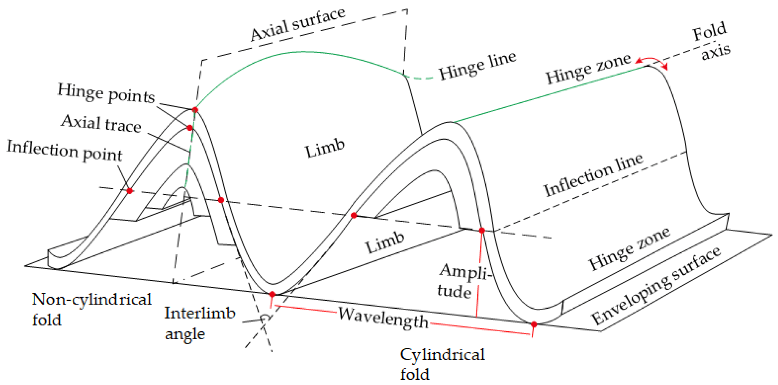
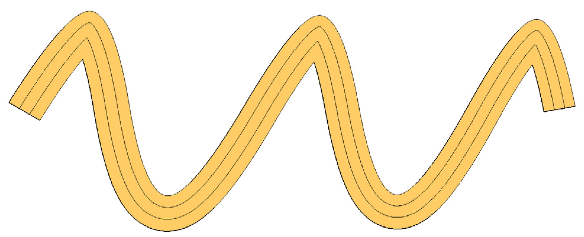
In general, fold structures not affected by strong denudation are wavy structures in shape [34] whose spatial morphology can be described by fold elements, such as limbs, hinges, and axial surfaces [42,43,44]. The limb refers to the rock strata on both sides of the core, the hinge is the connecting line of the maximum bending point on each cross-section of the fold, and the axial surface refers to the surfaces formed by connecting the hinge lines on each adjacent fold stratum (Figure 1).
The formation mechanism of the folds is closely related to their stress mode and deformation environment and the deformation behavior of the rock stratum [44]. The diversity of fold formation mechanisms determines the complexity of the fold structures and the diversity of the fold types. Different types of folds are mainly classified according to their position, axial occurrence, and section morphology (Table 1).
Due to the lack of borehole data in the fold structure development area, generating a series of cross-cutting sections based on geological maps, and using the contour comparison algorithm [45] to build a 3D model of the fold structure, is the most feasible method. The two critical points of this method are to reasonably plan the location of the section lines based on the location parameters and to efficiently generate a series of cross-sections based on the section morphology parameters. First, the location parameter of the cross-section (Table 2) was mainly used to determine the location and strike of the cross-sections. The relevant parameters can be directly obtained from geological maps or geological structure maps. Second, the morphological parameters of the cross-section (Table 2) represent the primary information that controls the cross-sectional morphology. The relevant parameters mainly include the axial dip angle, interlimb angle, limb occurrence, and stratigraphic information. These parameters control the local details of each stratum in the cross-sections of the fold structure. The geometric characteristics of the different fold types can be constrained and controlled by the different value ranges of the fold morphology parameters.
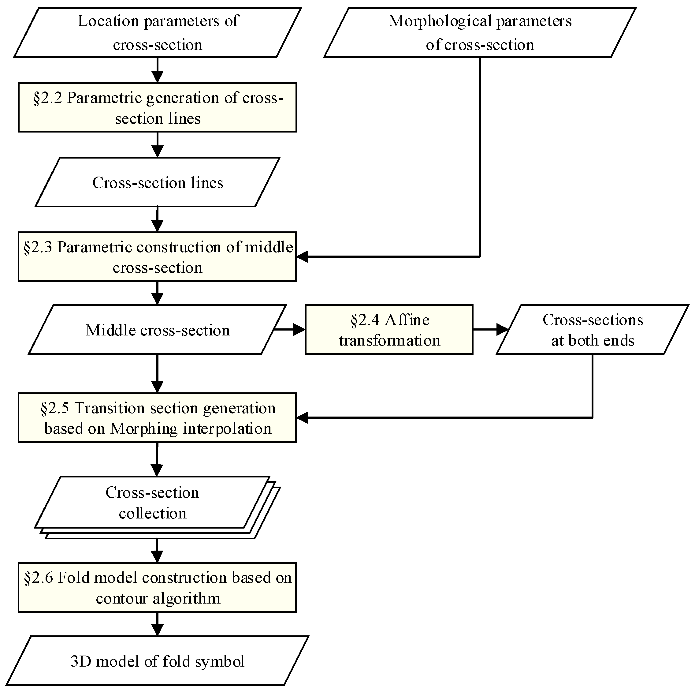
Based on the modeling parameters outlined above, this study presents a parametric 3D modeling method for fold symbols (Figure 2). The specific modeling steps primarily include: (1) the parametric generation of the cross-section lines based on the section location parameters; (2) the parametric generation of the middle cross-section based on the section morphology parameters; (3) the generation of the cross-cutting section at both ends based on the affine transformation; (4) the generation of the transition sections based on the morphing interpolation; and (5) the stitching and attribute assignment of the fold model.
2.2. Generation of Cross-Section Lines
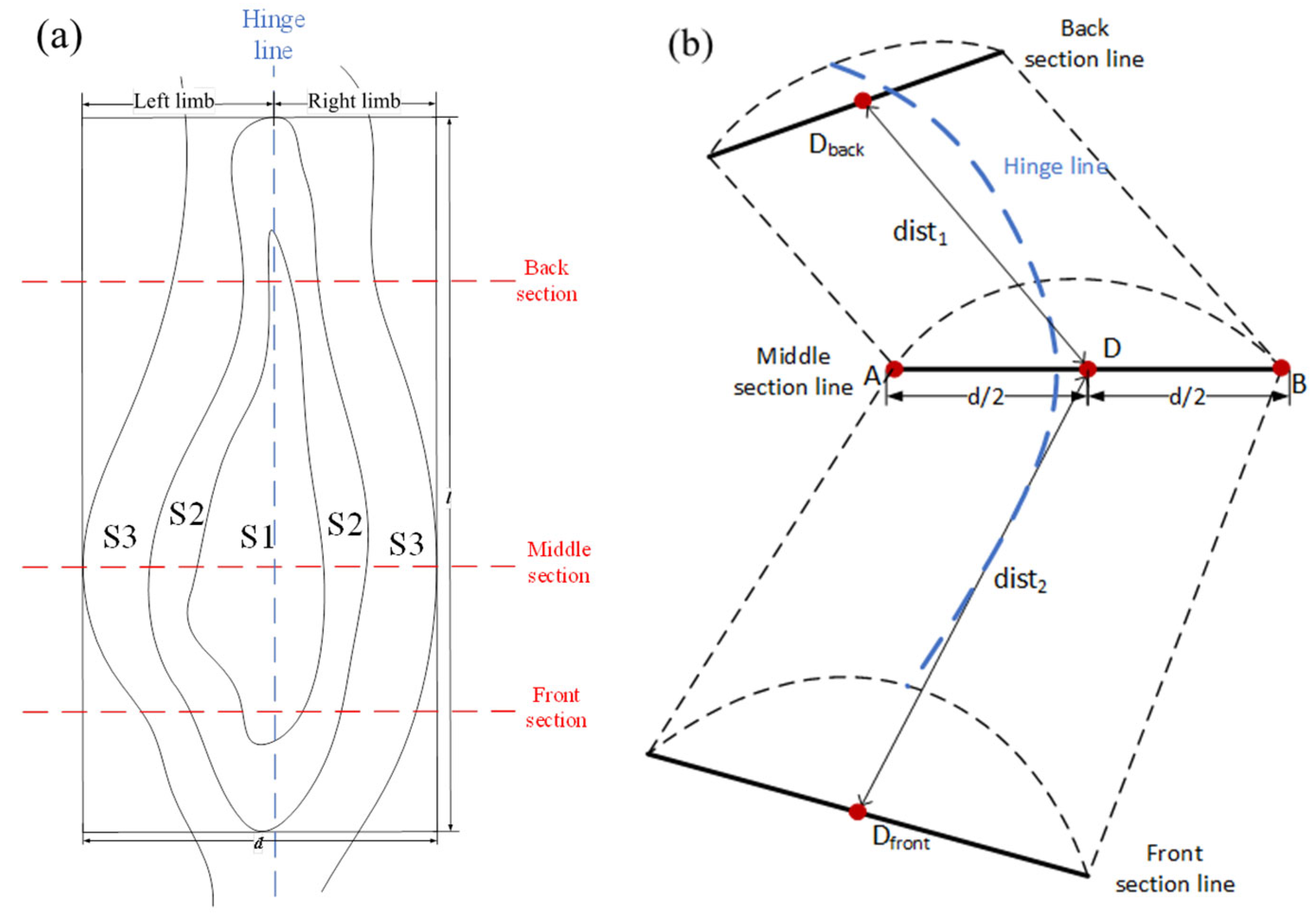
The premise of generating a 3D fold-symbol model based on a contour comparison algorithm is to generate cross-sections by locating each cross-section of the fold. The stratigraphic information in the cross-section of the fold structure should be comprehensive and reflect the typical characteristics of the fold structure. Therefore, the position of the cross-sections should be determined according to the distribution of various strata of the fold structure and the direction of the hinge line (Figure 3a). This process makes the symbol model closer to the actual situation of the structure, which implies a higher degree of model restoration.
Furthermore, to break through the excessive dependence on geological survey data, this study applies the premise of extracting section location parameters based on geological maps (Figure 3a) and mainly determines the location of cross-sections according to the modeling parameters input by users (Figure 3b). The specific steps are as follows: (1) take the center point D of the middle section, according to the position parameters as the midpoint, and extend, perpendicularly, to the average hinge line strike (hinge line in Figure 3a) to obtain the positions of inflection points A and B of the middle section at d/2; and (2) calculate the affine transformation coefficient and generate the positions of the section lines at both ends, according to the distances (dist1 and dist2) from the front and back sections to the middle section, the occurrence of the hinge line (including front and back strikes of hinge lines μ1 and μ2 and front and back dip angles of hinge lines δ1 and δ2) and dip angle of the axial surface of the front and back sections γ1 and γ2.
2.3. Construction of Middle Cross-Section
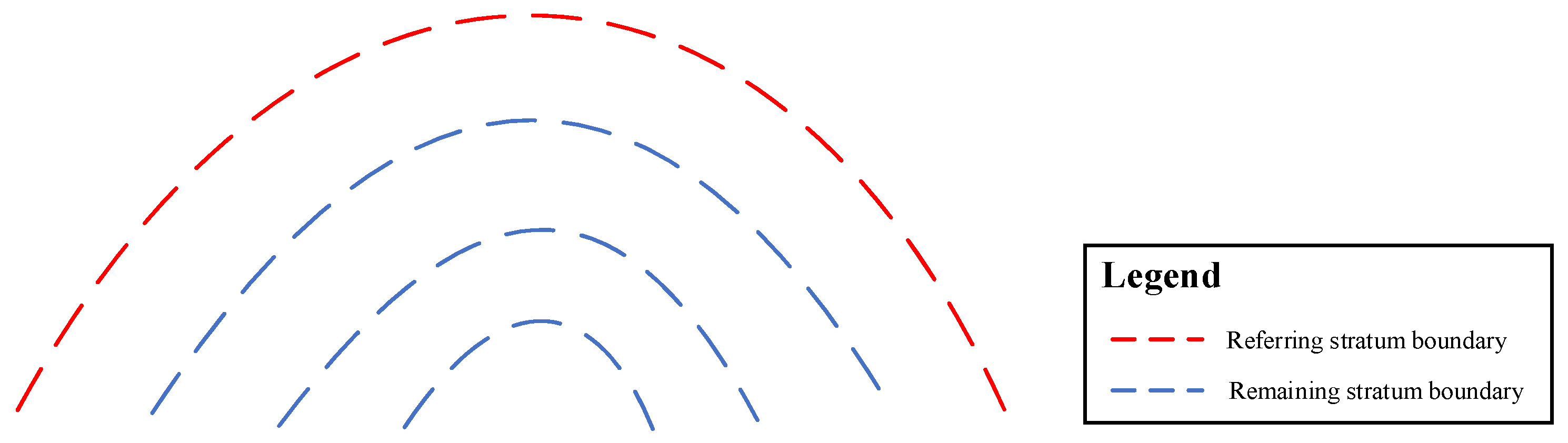
The construction of the middle cross-section is essentially the process of generating the boundary of each stratum based on the morphological parameters of the cross-section. According to the morphological consistency of different stratum boundaries in the cross-section, and based on the premise of generating one stratum boundary based on the parameters, this boundary can be used as the reference stratum boundary to deduce and generate other stratum boundaries. Therefore, the stratum boundary of the middle section can be divided into two types: the reference stratum boundary and the general stratum boundary (Figure 4). The boundary of the outermost stratum was generally selected as the reference stratum boundary. The generation of the stratum boundary mainly includes three parts: the generation of the reference stratum boundary; the deduction of the general stratum boundary; and the trimming of the stratum boundary.
2.3.1. Generation of Reference Stratum Boundary
The stratum morphology of the fold structure is generally smooth and regular and shows specific function laws, and it can be described in terms of amplitude and wavelength [42]. Therefore, it is feasible to use a quadratic Bessel curve to simulate the stratum boundary of the fold structure. In addition, folds are usually formed by the hinge zone and its two connected limbs, and the stratum morphologies of the two limbs tend to be different. Therefore, dividing the boundary line of the fold stratum into two segments according to the hinge zone is appropriate, and the Bezier curve is used to express this division [46,47]. In addition, the fitting of the Bezier curve was realized through the endpoints and control points. Suppose that only one segment of the Bezier curve is used for the fitting; in this case, obtaining the Bezier control points according to the shape of the interlimb angle is difficult, which causes the morphology of the hinge zone to not be precisely controlled. Therefore, the generation of the reference stratum boundary can be transformed into the selection of the Bezier endpoints and control points of the two curves.
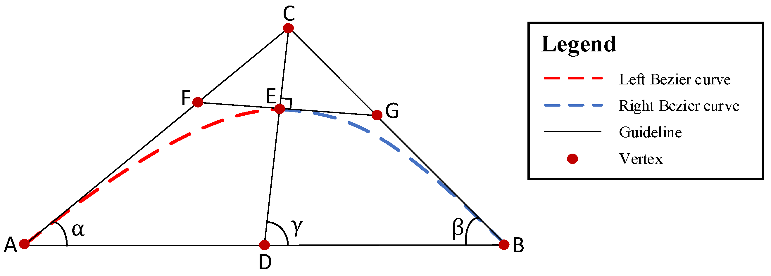
The generation of the reference stratum boundary mainly includes the following steps: (1) calculate the intersection point C of the tangent lines at the inflection points, according to the inflection points (A and B) of the middle section, and the dip angle of the two limbs (α and β) mentioned in the section morphological parameters; (2) find the intersection point D between the angle bisector of angles ACB and AB, and CD is the axial surface line of the middle section; (3) cut point E proportionally on CD as the hinge point, based on the morphological parameter curve; (4) extend the vertical line of CD through point E and intersect AC and BC to points F and G, respectively; and (5) take points A and E and points E and B as the endpoints, and F and G as the Bezier control points of the left and right curve segments, respectively, and then conduct segmented Bezier interpolation to obtain the reference stratum boundary (Figure 5).
2.3.2. Deduction of General Stratum Boundary
According to the principle of stratigraphic superposition [48], the bottom surface of each stratum in the fold structure is generally morphologically consistent. Therefore, if the bottom deduction rules of the reference stratum are determined, all the general stratum boundaries can be obtained. However, the deduction rules for the general stratum boundaries differ for different types of fold structures. Taking the isopach fold and similar folds as examples, the deductive method of the general stratigraphic boundary is briefly described below.
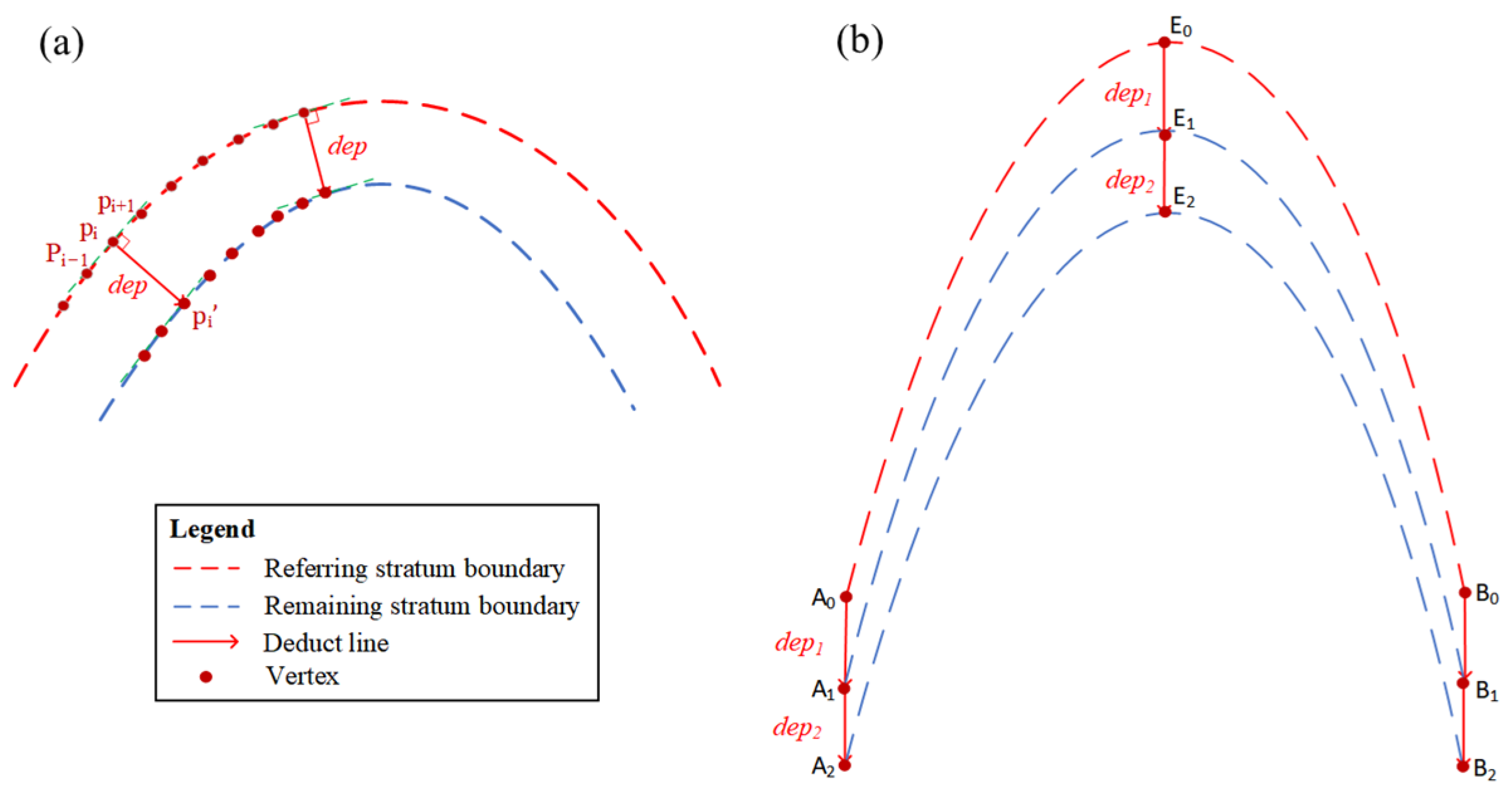
The isopach fold has typical characteristics and the “stratum thickness is equal everywhere” [42]. Deducing the general stratum boundaries in such a structure can be realized by moving a certain distance along the normal direction, according to the stratum thickness based on the points in the reference stratum boundary (Figure 6a).
The characteristic of a similar fold is that the curvature radius of each stratum boundary is similar, although a common curvature center is not observed [42]. In other words, the morphology of the stratum boundaries is the same, but their locations are different. Therefore, the general stratum boundaries can be obtained by translating the reference stratum boundary in the vertical direction, and the translation distance can be determined by the stratum thickness at the hinge zone (Figure 6b).
2.3.3. Trimming of Stratum Boundary
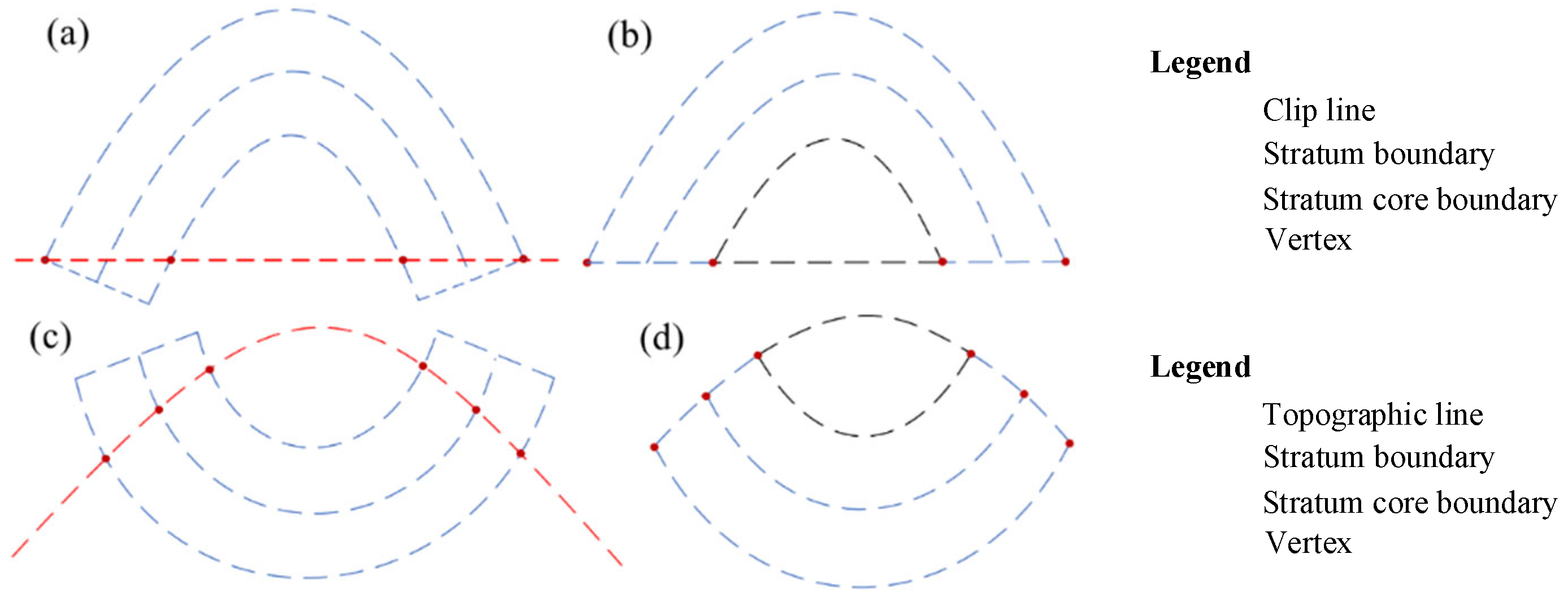
As with 2D geological symbols, 3D fold symbols should also be designed to convey geological information as simply as possible and by focusing on the aesthetic expression of symbols. During stratum deduction, the strata of the isopach fold are inferred according to the normal direction of the reference stratum boundary, resulting in uneven stratum boundaries. Therefore, for anticlinal folds with low openness, the bottom of the entire section must be trimmed based on the inflection points of the two limbs in the outermost stratum (Figure 7a,b). For the syncline, the topographic line at the section location was used as a trimming line to trim the top of each stratum to truly express the morphology of the stratum surface (Figure 7c,d). In addition, the core stratum should be calculated according to the principle of stratum superposition.
The specific steps of this method are as follows: (1) calculate the trimming line equation according to the inflection points of the middle section; (2) eliminate the points outside the trimming line in the stratum boundary of each stratum; (3) supplement the points on the trimming line in the stratum boundary of each stratum by linear interpolation; and (4) generate the core stratum boundary according to the area enclosed by the trimming line and the bottom stratum (Figure 7c,d).
2.3.4. Section Treatment for Special Fold Types
The parametric modeling method of the cross-section described above mainly applies to types of folds where no inversion occurs. Thus, the distorted and deformed morphology of overturned or recumbent folds must be optimized on this basis.
- (1)
- Overturned fold
The two limbs of the overturned fold inclined in the same direction, and one of the limbs was overturned. The stratum boundary generation method in Section 2.3.1 can be used to construct the stratum boundaries by treating the dip angle at the overturned limb as an obtuse angle (Figure 8a). However, owing to the compression and deformation between strata, most of the strata of the overturned folds will be distorted to varying degrees [49]. Therefore, when constructing the middle cross-section, the rotation angle of the section point set around vertex D can be calculated according to Formula (1). Distortion and deformation processing are then carried out to realize an approximate simulation of the overturned fold morphology.
where amax is the maximum rotation angle, R is the maximum rotation radius, r is the distance from the current point to the rotation center D, and θ is the angle of rotation required for the current point.
θ = amax × (R − r)/R
- (2)
- Continuous fold belt
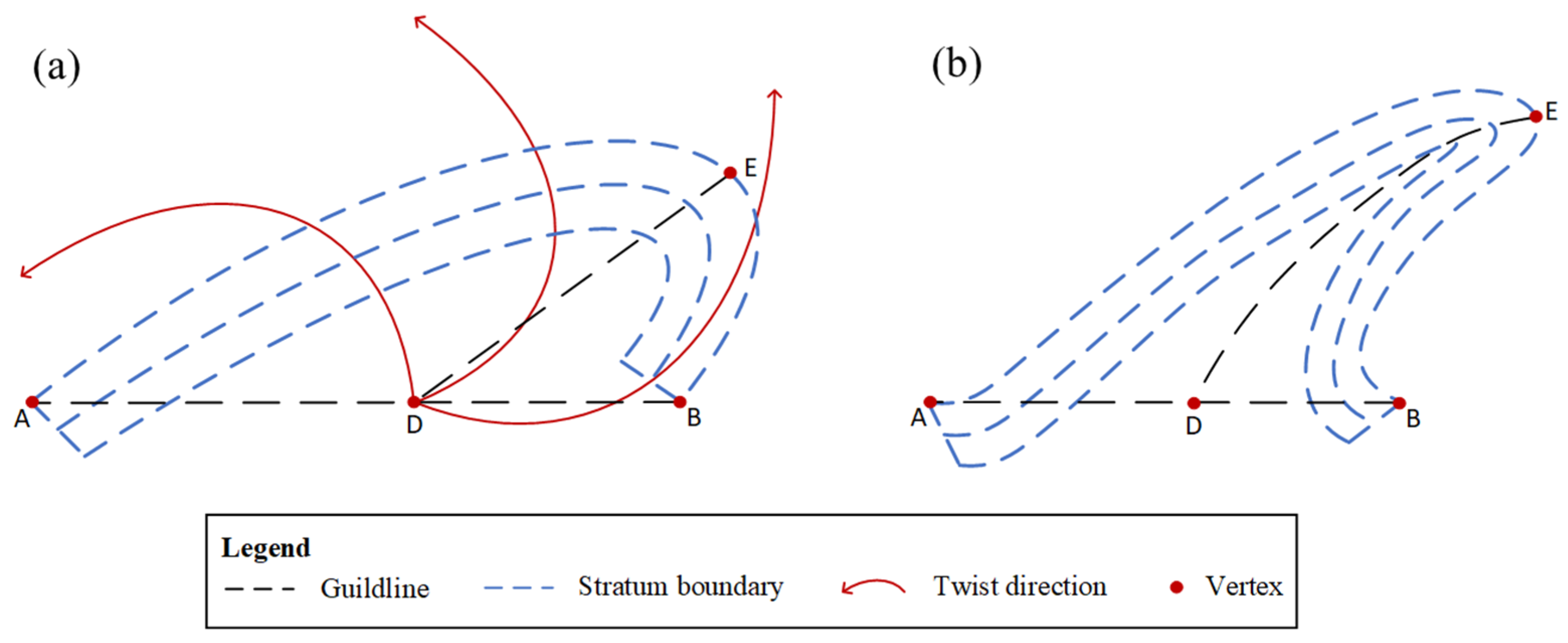
In general, typical geological structures with prominent characteristics are often accompanied by large-scale folding activities. One single symbol model of a fold cannot easily reflect the structural characteristics of a continuous fold belt. To enable fold symbols to effectively realize the abstract expression of geological characteristics under different geological scales, this study uses the periodic cycle method to repeat the middle section construction steps presented in Section 2.3 to generate the cross-section of continuous fold belts (Figure 9).
2.4. Generation of Cross-Sections at Both Ends
Based on the morphological consistency among cross-sections of the fold structure, the cross-sections at both ends can be obtained by affine transformation from the middle cross-section. The affine transformation in this section includes translation, magnification, and rotation. The strike of the hinge affects the offset distance of the sections at both ends along the X-axis, the dip angle of the hinge affects the magnification ratio of the sections at both ends, and the dip angle of the axial surfaces of the sections at both ends affects the rotation angle. The specific affine transformation parameters and corresponding calculation methods are listed in Table 3.
2.5. Generation of Transition Sections
The cross-sections, including the front, middle, and back, were obtained. Theoretically, these cross-sections can be stitched directly to complete the rough construction of the entire fold model. However, the spatial morphology of the hinge line is difficult to express using this method, which affects the accuracy and aesthetics of the model results to a large extent. Therefore, many transition sections need to be generated through morphing interpolation according to these cross-sections to realize the fine modeling of the fold symbol.
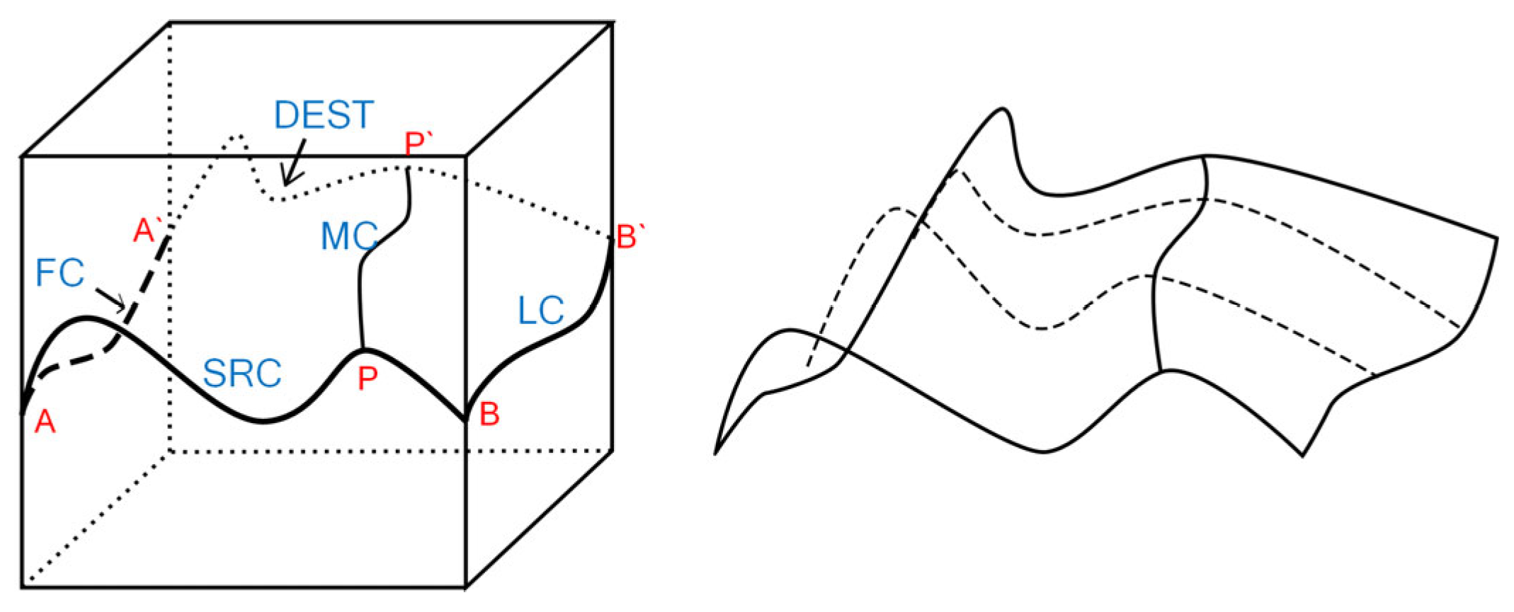
Morphing is an interpolation technique that smoothly transitions an initial object into a target object. This technology has been widely used in animation production, virtual reality, image compression, and image reconstruction [50,51,52]. Three types of boundaries are necessary for morphing interpolation (Figure 10): (1) the starting boundary with direction (SRC); (2) the target boundary (DEST) with a direction that must be consistent with that of SRC; and (3) the first and last constraint boundaries with directions (FC and LC) [53].
2.5.1. Selection of Constraint Boundaries
Considering that the monotony of a single fold element in a folded section will experience one change at the hinge zone [54], this study considers the hinge line as the middle constraint and divides the strata of the fold sections into left and right parts. Morphing interpolation with four boundaries intersected by the hinge line was performed for the two limbs. This method allows the hinge information to participate effectively in the morphing interpolation process, thus ensuring the accuracy of the overall interpolation result.
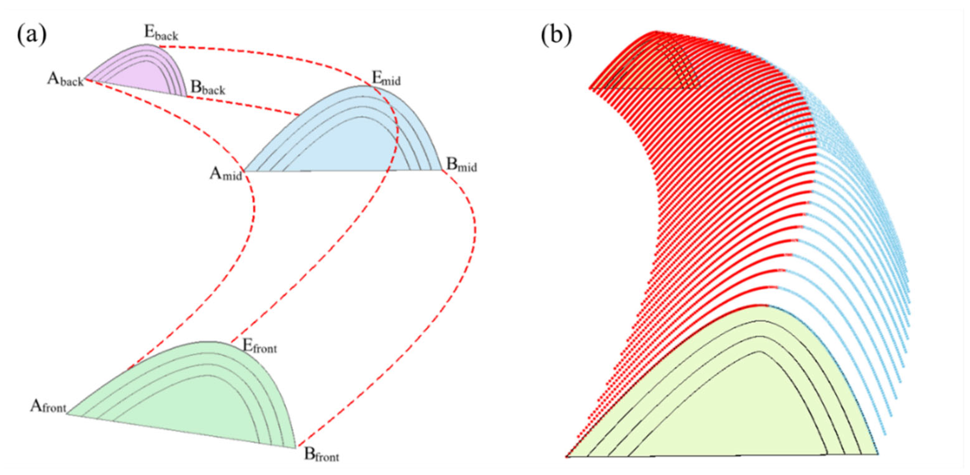
Among the four constraint boundaries of the morphing interpolation method, the starting and ending stratum boundaries, SRC and DEST, can be obtained from the stratum boundary on the corresponding limb [46]. To make the section transition smoother, the constrained stratum boundaries, FC and LC, must be obtained by interpolation according to the corresponding characteristic points of each section. By connecting the points generated by the Lagrange interpolation results of A, E, and B (i.e., left inflection point, hinge point, and right inflection point, respectively), three smooth curves (AfrontAmidAback, EfrontEmidEback, and BfrontBmidBback) of each stratum surface can be obtained (Figure 11a).
2.5.2. Transition Section Generation Based on Morphing Interpolation
Calculate any point M (u, v) inserted in the transition section according to the morphing formula (2), and then obtain the point set of the transition section.
where M (u, v) represents the point to be inserted, and it is jointly controlled by the transverse path interpolation function H (u, v) and longitudinal constraint boundary function L (u, v). 0 ≤ u ≤ 1, 0 ≤ v ≤ 1. Moreover, as shown in Figure 10, u represents the close degree between the point to be inserted and the FC or LC constraint lines and v represents the close degree between the point to be inserted and SRC or DEST lines. In addition, F(u) is the curve function of the SRC, G(u) is the curve function of the DEST, P(v) is a function of FC and Q(v) is a function of LC, a is the adjustment factor corresponding to the FC, and b is the adjustment factor corresponding to the LC.
2.6. Fold Model Construction and Attribute Assignment
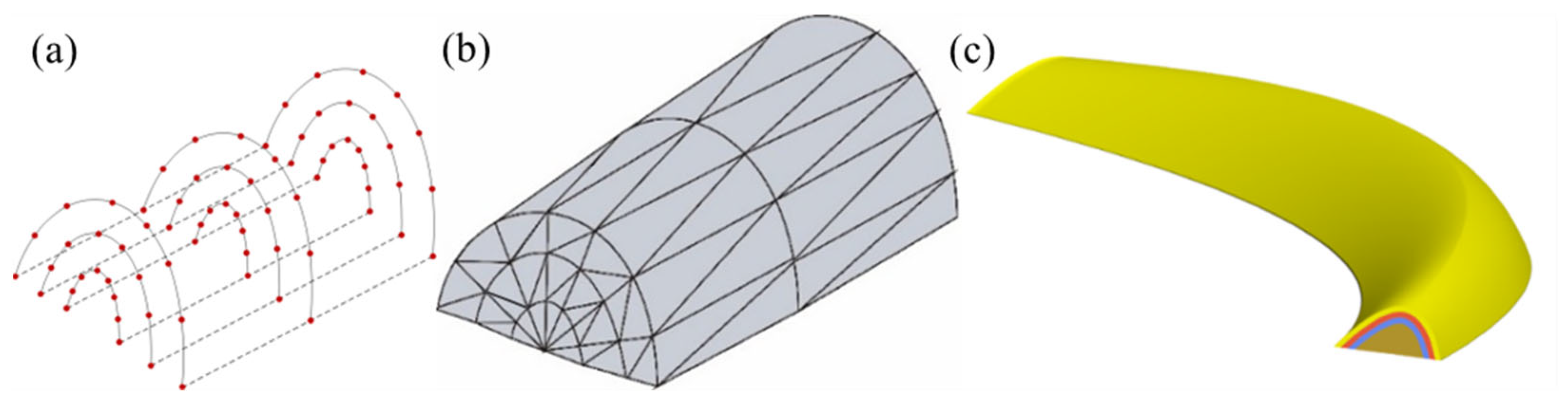
After the construction of all of the transition sections is completed, the boundary representation (Brep) surface model of the fold symbol can be built based on the contour comparison algorithm [55]. The difficulty of the contour algorithm lies in the treatment of branching, correspondence, meshing, and smoothing problems [56]. For the method used in this study, because the point sets between adjacent sections are all in one-to-one mode, the branching problem and corresponding problem are not observed. The smoothing problem can also be solved by generating transition sections.
Considering the facet complexity and algorithm efficiency of the modeling result, the shortest diagonal method is selected [57] (Figure 12b). This is a locally optimal objective function method. The fold symbol model was finally obtained based on the contour comparison algorithm, as shown in Figure 12c.
After the model stitching is completed, attribute information, such as age, the lithological description of each stratum, and contact relationship between strata, can be stored in the corresponding JSON format model attribute file. The association query between the 3D model and the attribute information, 3D information annotation, and other functions can be effectively performed by binding the ID information of each object.
3. Case Studies
This study selects four folds with different types for testing the performance of the 3D modeling of fold-structure symbols. The experiments were carried out using a computer with the configuration of a 3.20 GHz Intel(R) Core (TM) i7-8700 CPU, 16 GB RAM. The operation system is Windows 10 Professional. All algorithms are implemented using GDAL3.2 and Dotspatial 1.8 and compiled using Microsoft visual C# 2017 compiler. The number of control and transition sections in all cases is three and eight, respectively. Information for each fold is presented in Table 4. The parameters of the different cases are summarized in Table 5.
3.1. Case 1: Anticline Modeling
Dayue Mountain is located southeast of Mount Lu in Jiangxi Province and represents the second highest peak in the Mount Lu region. The measured data from geological records of Mount Lu [58] indicate that the 3D symbol model of Dayue Mountain (Figure 13b), generated based on the above parameters, reflects the structural characteristics of Dayue Mountain, such as equal stratum thickness, vertical anticline, and rounded hinge zone. The number of vertices and triangles is 16,755 and 28,418, respectively.
3.2. Case 2: Modeling of Syncline
Danaobo Mountain, as an oblique horizontal fold, is located in the Xifeng Cave and Danaobo mountain area at the northeast corner of the survey area (Mahui Ridge sheet (H-50-88-D)). The axial trace is in the northeast direction, and the axis surface inclines to the southeast at a dip angle of approximately 70°. The hinge was nearly horizontal, the fold length was approximately 9 km, and the width was approximately 2.5 km. Among the strata involved, the core is the second and fourth member of the Hanyangfeng Formation and the two limbs are the first and second members of the Hanyangfeng Formation. The generated 3D symbol model of Danaobo Mountain is shown in Figure 14. The number of vertices and triangles is 14,539 and 29,062, respectively.
3.3. Case 3: Modeling of Chevron Anticline
The Fangdou Mountain chevron anticline is located in the East Sichuan Fold Belt. The mountain is a narrow, high, and steep anticline in the Jura-type folds of eastern Sichuan. The Fangdou Mountain structure is a composite anticline composed of fault-bend folds and longitudinal-bend folds controlled by detachment, and its surface section is an asymmetric fold with a sharp hinge zone, which gradually widens and slows to form an asymmetric box fold [62]. According to the 95-23.5 survey line section data of Fangdou Mountain [60], the limb dip angles of the anticline are approximately 20°–25° and symmetrical and the axial surface is nearly vertical. Based on these parameters (Table 5), a 3D symbol model of Fangdou Mountain (Figure 15) is generated, which reflects the structural characteristics of its anticline, sharp edge, upright, and symmetrical characteristics. The number of vertices and triangles is 12,843 and 24,748, respectively.
3.4. Case 4: Modeling of Recumbent Folds
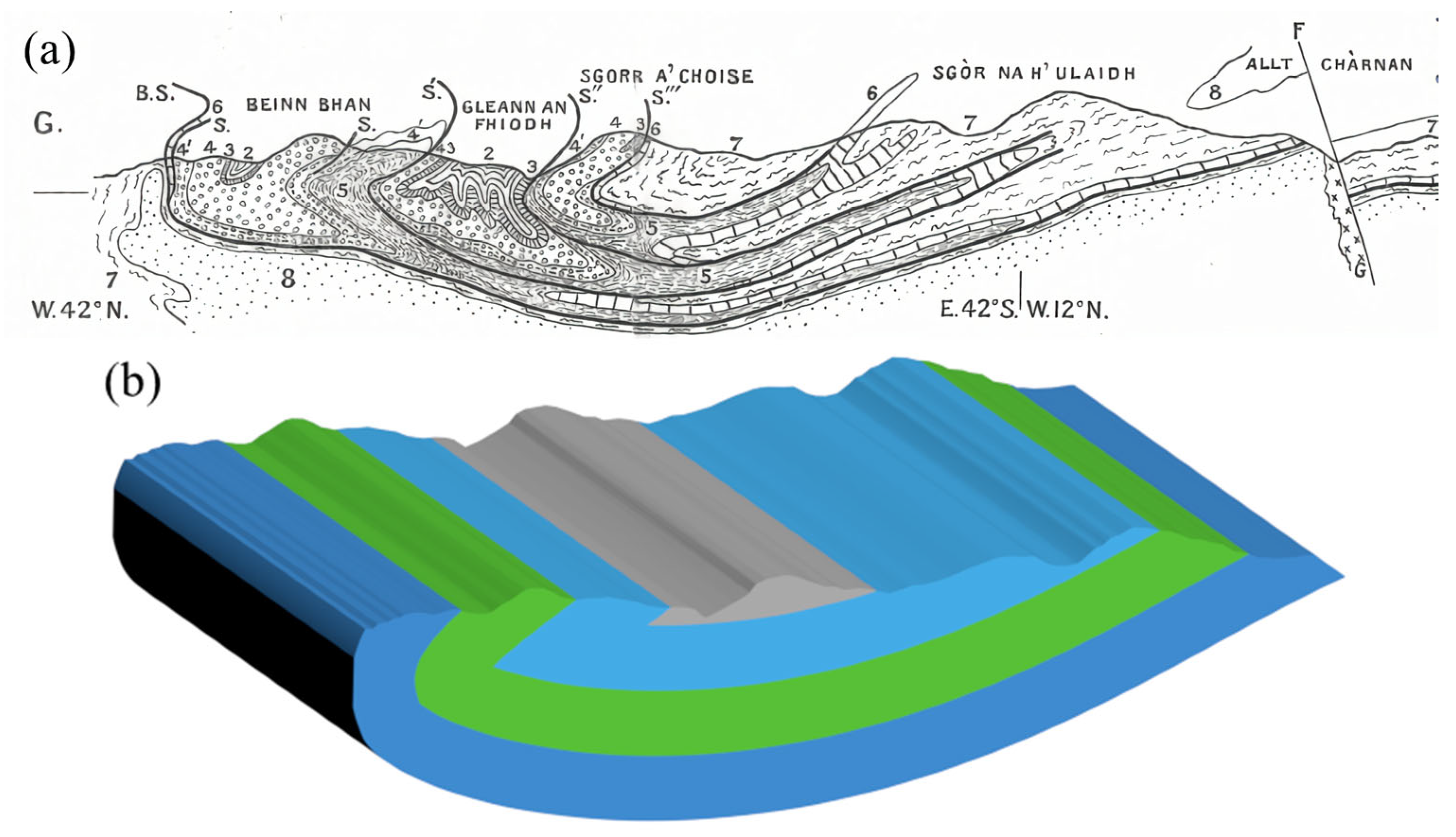
A large number of overturned folds are observed in the Scottish Highlands [61]. This study selects a recumbent fold to demonstrate symbol modeling in the central south zone of the area. The approximate fold information can be obtained from the geological section map (Figure 16a): the dip angle of the left limb was approximately 150° and the right is at approximately 10°. The generated 3D symbol model is shown in Figure 16b. The number of vertices and triangles is 7020 and 14,024, respectively.
3.5. Case 5: Other Types of Folds
In addition to the fold structures in the specific areas mentioned above, this method can also be applied to a more general fold symbol modeling based on the inclusion of the appropriate modeling parameters. When the morphological parameter cur is set to 0.8, 0.5, and 0.2, the symbol models of the chevron fold, circular fold, and box fold can be generated. When the interlimb angle θ is set to 30°, 50°, 100°, and 160°, the symbol models of a tight fold, closed fold, broad fold, and gentle fold can be generated, respectively (Figure 17).
4. Discussion
4.1. Analysis of the Influencing Factors
The use of a greater number of control sections increases the accuracy of the generated model and ensures that the model is able to better restore the morphological characteristics of the fold structure. For fold structures with small-scale and prominent characteristics, fewer control sections are required to reflect the hinge morphology. In contrast, for fold types with large-scale and relatively complex hinge morphologies, more control sections are required. The typical fold structure selected in this experiment has a small scale; therefore, only three sections in the middle and at both ends were generated.
The use of a greater number of transition sections leads to the generation of a smoother model and requires a greater amount of model data. However, the running efficiency tends to be lower when a model with a large amount of data displays a large scene. For the fold type with a relatively smooth hinge zone, fewer transition sections are required to effectively reflect the 3D morphology of the fold structure. Otherwise, more transition sections would be required to effectively reflect the 3D morphology of the fold structure.
The different selection methods of the location parameters of the cross-sections significantly influence the model morphology. The location parameters of the cross-sections can be measured based on the outer rectangle of the fold distribution range or the outer rectangle of the core formation. These methods can be applied as long as they can effectively reflect the morphological characteristics of the fold structures.
The quality of the middle cross-section is a critical factor for determining the modeling quality of the fold symbol. The parametric modeling method is effective for the middle cross-section with a relatively simple stratum boundary morphology. However, the effect of parametric modeling is poor for a more complex middle cross-section. In this case, a better modeling quality can be obtained by replacing the cross-sections generated by the parameters with the measured cross-section.
4.2. Factors That Influence the Symbol Display Effect
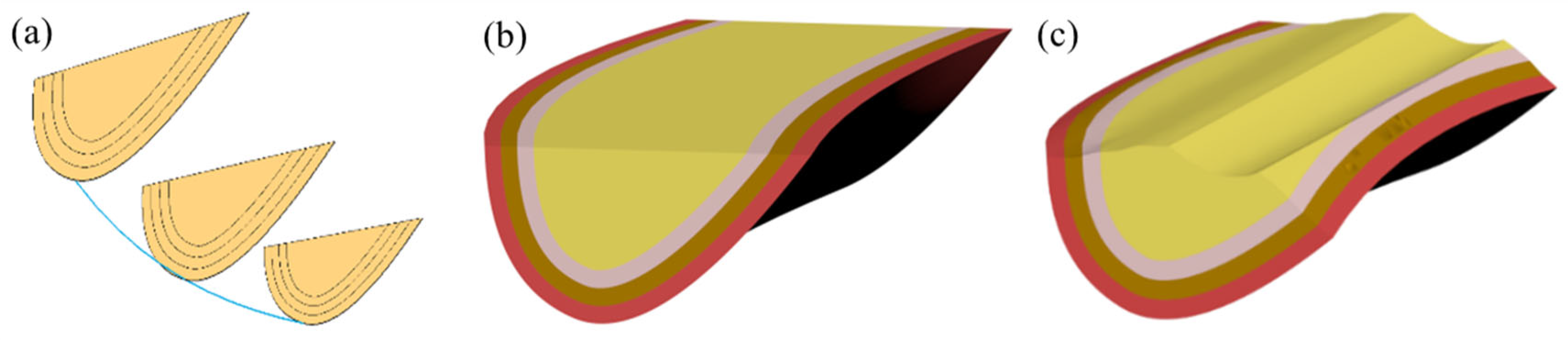
The spatial information of the constructed models is stored in an OBJ format file, while the attribute information is in JSON. The constructed 3D fold symbols can be placed on a 3D Earth display platform (such as Cesium or Google Earth). When importing a model into Cesium, the process mainly includes: (1) converting the OBJ format model file to FBX format file, which contains information such as material and lighting; (2) converting the FBX format model files to GLB format file, which is the 3D model data format supported by the Cesium platform; (3) directly loading the glb file into the Cesium scene.
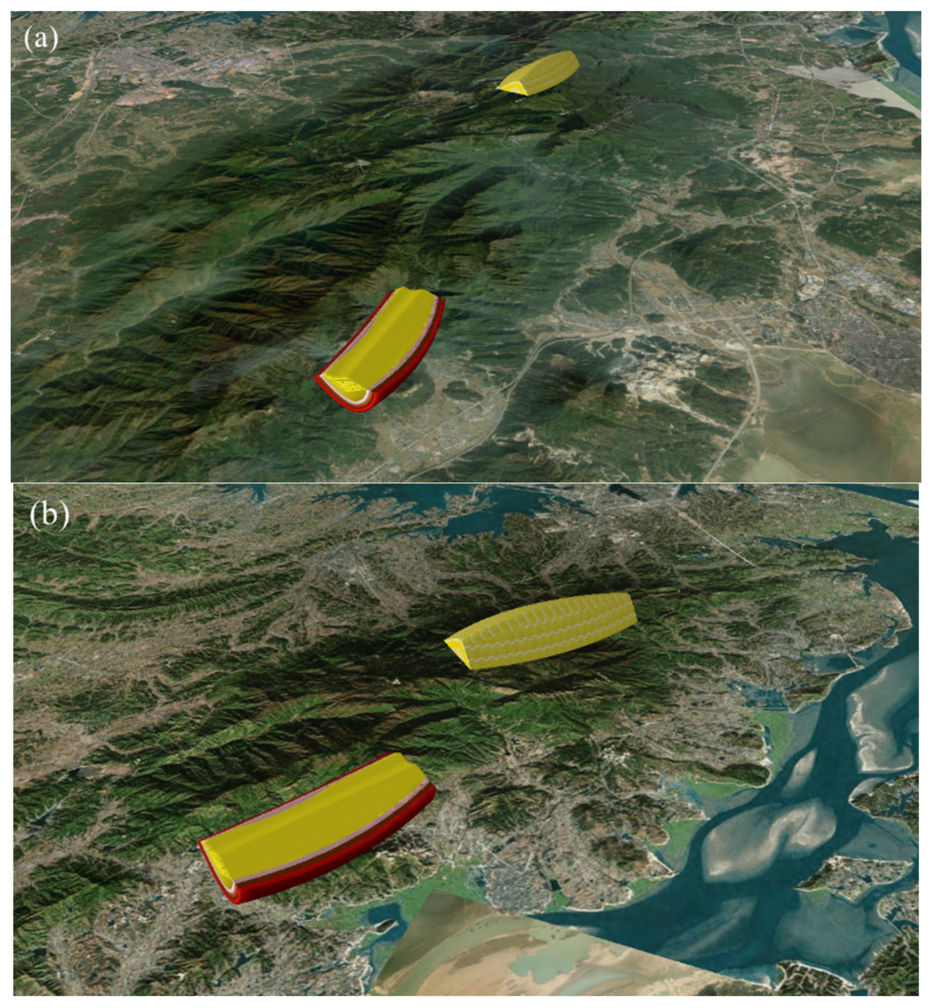
Consistent with the expression requirements of 2D symbols [63], when the constructed 3D folding symbols are placed on the 3D earth display platform, it is also necessary to set the appropriate symbol size to optimize the display effect. When the scale of the fold structure is small and the internal characteristics of the fold elements are apparent, the effect is better when the ratio of the symbol to the actual fold is 1:1. When the scale of the fold structure is large, the internal characteristics of the fold elements will not be sufficiently prominent, and the effect of the proportional magnification will be better. In addition, in 2D electronic maps, the size of related symbols usually needs to be adaptively adjusted at different scales. This rule also applies to symbol-size settings in 3D scenes. For example, when displayed on the Cesium platform, the size of the corresponding model can be changed for adaptive scaling and adjustment to ensure that the relative size of the symbol model remains unchanged at different scales (Figure 18).
When the symbol is smaller than the actual geological structure, it should be placed directly above the center point of the actual geological structure. When the scale is 1:1, the symbol should be placed in the actual position of the structure and the height should be consistent with the actual structure. In addition, when symbols are placed, the strike of the symbols must be consistent with that of the actual structure.
Different proportions may occur between the actual length along the hinge direction and the width of the fold structure. According to the ratio of longitudinal length to transverse width, folds can be divided into linear, long-axis, short-axis, or equiaxed folds (dome structure and tectonic basin) [64]. However, if the symbol model is constructed according to the actual proportion of the geological structures, then the structural information conveyed by the fold elements is weakened and the information about the hinge zone is highlighted. Moreover, the typical geological characteristics of some ample linear folds are likely to be reflected in the spatial information of the hinge; thus, comprehensive restoration of the entire fold is also required. Therefore, intercepting a part of the fold in the hinge direction or reflecting the 3D morphology of the entire fold depends on the characteristics of the fold and preferences of the user (Figure 19).
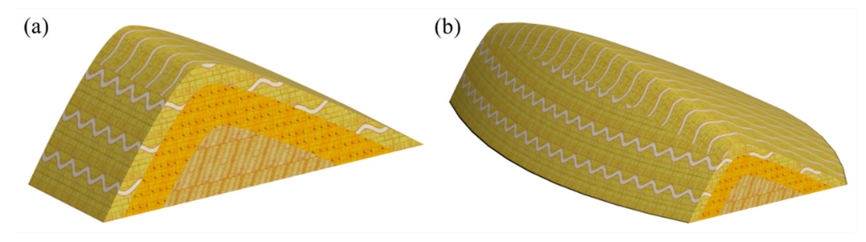
Stratigraphic legends usually use color to indicate age and texture to indicate lithology. Therefore, by using an appropriate legend to decorate the corresponding strata, the fold symbols can better express and transmit the age and lithology information.
4.3. Analysis of Applicability
The premise of parametric modeling is to obtain relevant modeling parameters effectively. In this method, the modeling parameters of the fold structure can be directly obtained from the regional geological survey report or measured from corresponding maps, such as geological maps, structural maps, or section maps. Under exceptional circumstances, the parameters required for fold modeling can also be empirically assigned according to the fold type and structural knowledge.
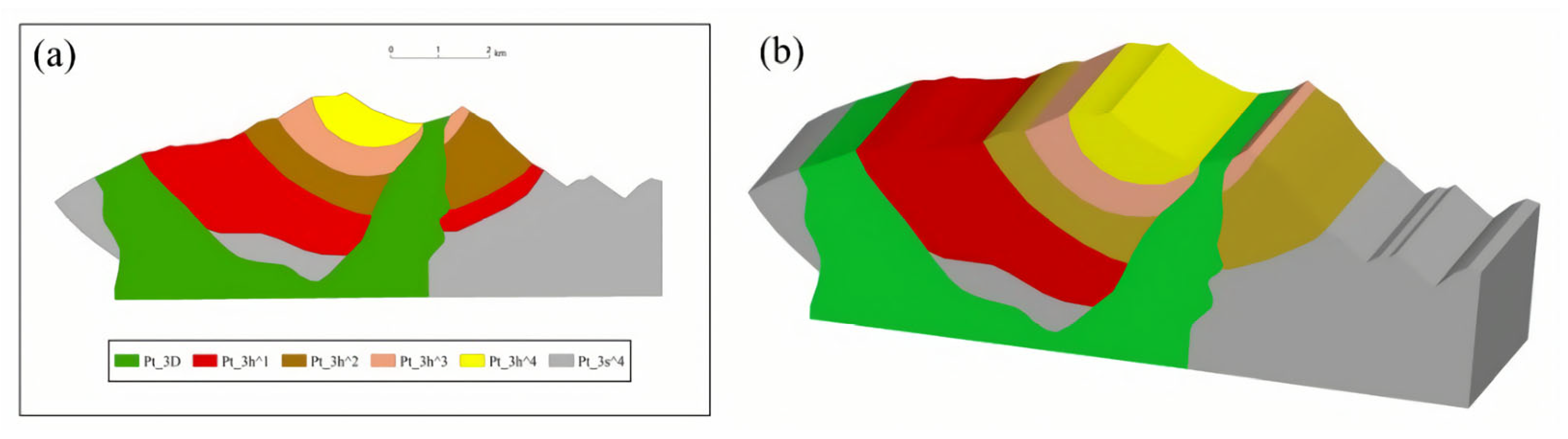
This study’s 3D parametric modeling method of fold symbol construction can realize symbol model construction when the geological data are insufficient. Although the symbol has an abstract requirement for the model structure, less dependence on geological data also means that the model results will be simplified in terms of morphology and large discrepancies with the actual structure may occur. In the case of complex sections, if the measured cross-sections are available, they can be used to replace the cross-sections generated by the parameters, so that more accurate modeling of the fold symbol can be carried out [23,24,25]. For example, by selecting the cross-section (Figure 20a) of the Danaobo mountain syncline as the middle section, a more detailed symbol model of the Danaobo mountain syncline can be built (Figure 20b). This experiment shows that the symbol model of the fold structure based on the measured cross-section can restore the actual morphology of the current fold structure. This method also has some shortcomings, such as relying on geological section data and being unable to directly reflect the original structural morphology before being subjected to external forces. In specific applications, the appropriate method for the cross-section can be selected according to the geological data and requirements to achieve the best data utilization and model expression effect.
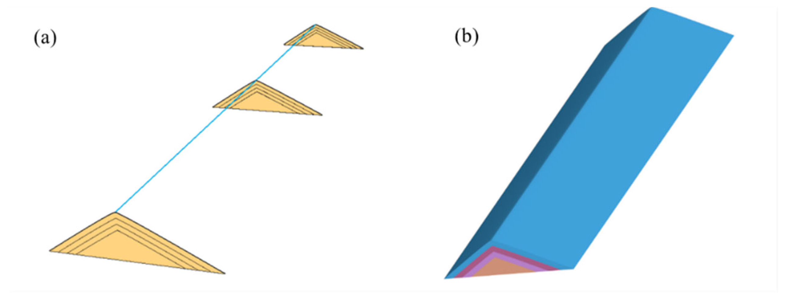
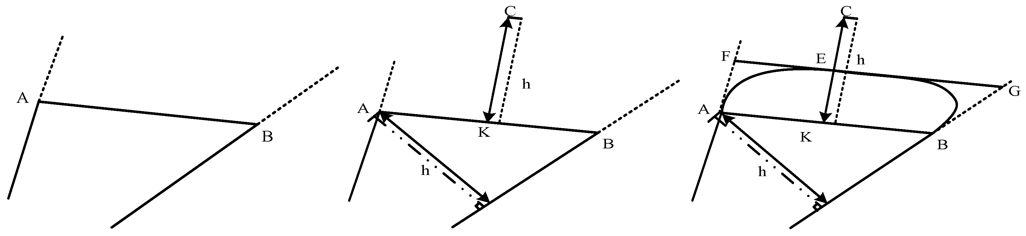
A box fold refers to a fold in which the strata are all overturned, and the hinge zone is flat and wide, similar to a box [64]. The box fold is a component of the world-famous Jura-type folds [65], which were developed in East Sichuan in China as well as in the Alps in Europe. In contrast to general folds, box folds typically have two hinges and a pair of conjugate axial surfaces. The parametric modeling method of fold symbols proposed in this paper cannot easily and directly realize the symbol modeling of box folds; therefore, a particular modeling method must be designed for box folds. According to the morphological characteristics of “two hinges and a pair of conjugate axial surfaces” of box folds, the middle cross-section of a box fold can be divided into left and right parts for modeling, and the topological transition at the middle junction should be guaranteed (Figure 21). The construction method of the stratum boundaries in the middle section of the box fold is as follows: (1) obtain the positions of inflection points A and B and the corresponding extension lines along the dip angles, according to the position of the inflection points and the occurrence of both limbs input by the user; (2) calculate the distance h from A to the extension line of B, take the midpoint K of AB, and make CK⊥AB so that the length of segment CK is equal to h; and (3) take point E on CK, according to the morphological parameter cur entered by the user, make FG//AB so that the dip extension lines of the two inflection points intersect with points F and G. After that, Bezier interpolation is carried out according to points A, F, E, E, G, and B to obtain the stratum boundary of the box fold; namely, the arc AEB.
A lack of apparent regularity is observed among stratum boundaries for more complex disharmonious folds. Rather than being deduced from a specific stratum boundary, the boundary of each stratum must be generated using the method described in Section 2.3.1. Therefore, the morphological parameters of each stratum of the disharmonious fold (such as the occurrence of inflection points, dip angles of the axial surfaces, and interlimb angles of each stratum) must be given in detail.
5. Conclusions
This study aims to develop a novel parametric modeling method for the 3D symbols of fold structures using cross-sections generated by fold parameters and a contour comparison algorithm. The cross-section generation method based on parameters and the Bezier curve effectively supports the parametric modeling of cross-sections of various fold structures. Transition section generation based on morphing satisfies the smooth requirement of the symbol model. The symbol-modeling method can control the model accuracy and data size by setting an appropriate number and quality of cross-sections, which may be measured or generated by fold parameters.
In this study, different types of fold structures were selected as experimental objects for modeling experiments. The experimental results show that the generated 3D fold symbol models can abstractly express the morphologies of fold structures developed in the experimental area and can express most fold structure subdivision types. The parametric modeling method for the 3D symbols of fold structures follows the traditional symbol creation rules [66] and cartographic rules [67]. The modeling method in this study is simple and efficient, avoids excessive dependence on geological survey data, and fits well with the abstract character of the geological symbol. Furthermore, the controllable characteristics of model accuracy and data size better meet the needs for efficient display in a wide range of 3D scenes.
In view of the inherent non-parametric geometric features of geological structures [41], this method breaks through the application limitation of parametric modeling methods in the field of 3D geological modeling. The parametric modeling method used for 3D fold-symbol modeling in this study can be applied for 3D symbol modeling of other geological structure types, such as faults, joints, and intrusions. It also applies for the 3D modeling of typical geological structures with relatively simple spatial morphology. The 3D geological symbols generated by this method have excellent research significance and application value for the 3D symbol expression of geological structures in digital Earth, digital cities, AR\VR\MR, geography teaching, science popularization, and other applications and research areas. In addition, the method in this paper has laid a sound data foundation for future research on the construction method of 3D spatio-temporal geological symbols (4D geological symbols).
Author Contributions
An-Bo Li conceived the original idea and is the primary author of the manuscript. Hao Chen developed the main modules of the prototype system and is the key contributor to the methodology. Xian-Yu Liu and Xiao-Feng Du developed partial modules of the prototype system. Guo-Kai Sun processed the relative data. All authors have read and agreed to the published version of the manuscript.
Funding
This study was supported by the National Key R&D Program of China (No. 2022YFB3904101, 2022YFB3904104) and by the National Natural Science Foundation of China (Project No. 41971068, 41771431).
Institutional Review Board Statement
Not applicable.
Informed Consent Statement
Not applicable.
Data Availability Statement
Not applicable.
Conflicts of Interest
The authors declare no conflict of interest.
References
- Declan, B. Virtual globes: The web-wide world. Nature 2006, 439, 776–779. [Google Scholar]
- Matrone, F.; Colucci, E.; De Ruvo, V.; Lingua, A.; Spanò, A. HBIM in a semantic 3D GIS database. Int. Arch. Photogramm. Remote Sens. Spat. Inf. Sci. 2019, 42, W11. [Google Scholar] [CrossRef] [Green Version]
- Landeschi, G.; Dell′Unto, N.; Lundqvist, K.; Ferdani, D.; Campanaro, D.M.; Touati, A.-M.L. 3D-GIS as a platform for visual analysis: Investigating a Pompeian house. J. Archaeol. Sci. 2016, 65, 103–113. [Google Scholar] [CrossRef]
- Petrov, V.A.; Veselovskii, A.V.; Kuz’mina, D.A.; Plate, A.N.; Gal’berg, T.V. Spatial-temporal three-dimensional GIS modeling. Autom. Doc. Math. Linguist. 2015, 49, 21–26. [Google Scholar] [CrossRef]
- Zhu, Q. 3D GIS and its application in smart cities. J. Earth Inf. Sci. 2014, 16, 151–157. [Google Scholar]
- Zhu, L.; Hou, W.; Du, X. Digital Earth—From surface to deep: Introduction to the Special issue. Front. Earth Sci. 2022, 15, 491–494. [Google Scholar] [CrossRef]
- Goodchild, M.F.; Guo, H.; Annoni, A.; Bian, L.; de Bie, K.; Campbell, F.; Craglia, M.; Ehlers, M.; van Genderen, J.; Jackson, D.; et al. Next-generation Digital Earth. Proc. Natl. Acad. Sci. USA 2012, 109, 11088–11094. [Google Scholar] [CrossRef] [Green Version]
- Gede, M.; Jeney, J. Thematische Kartierung mit Verwendung von Cesium Thematic Mapping with Cesium. KN J. Cartogr. Geogr. Inf. Kartogr. Nachr. 2017, 67, 210–213. [Google Scholar] [CrossRef]
- Gual, J.; Puyuelo, M.; Lloveras, J. Three-dimensional tactile symbols produced by 3D Printing: Improving the process of memorizing a tactile map key. Br. J. Vis. Impair. 2014, 32, 263–278. [Google Scholar] [CrossRef]
- Holloway, L.; Marriott, K.; Butler, M. Accessible maps for the blind: Comparing 3D printed models with tactile graphics. In Proceedings of the 2018 Chi Conference on Human Factors in Computing Systems, Montreal, QC, Canada, 21 April 2018; pp. 1–13. [Google Scholar]
- Bandrova, T. Designing of Symbol System for 3d City Maps. In Proceedings of the 20th International Cartographic Conference, Beijing, China, 2016. [Google Scholar]
- Patton, J.C. SOME Truth with Maps: A Primer on Symbolization and Design. Cartogr. Perspect. 1995, 20, 46–47. [Google Scholar] [CrossRef]
- Zhu, S.R.; Liu, B.B.; Chen, F.X. Automatic 3D modeling of 2D geological vector point symbols. Surv. Mapp. Sci. 2017, 42, 132–138+146. [Google Scholar]
- Lemon, A.M.; Jones, N.L. Building solid models from boreholes and user-defined cross-sections. Comput. Geosci. 2003, 29, 547–555. [Google Scholar] [CrossRef]
- Wei, Y.J. Research on the Organization, Management and Symbolization of 3D GIS Data. Ph.D. Thesis, PLA Information Engineering University, Zhengzhou, China, 2006. [Google Scholar]
- Fernández, O. Reconstruction of Geological Structures in 3D: An Example from the Southern Pyrenees. Ph.D. Thesis, Universitat de Barcelona, Barcelona, Spain, 2004. [Google Scholar]
- Laurent, G.; Ailleres, L.; Grose, L.; Caumon, G.; Jessell, M.; Armit, R. Implicit modeling of folds and overprinting deformation. Earth Planet. Sci. Lett. 2016, 456, 26–38. [Google Scholar] [CrossRef]
- Rife, D. Acoustic analysis and visualization using real time three-dimensional parametric modeling. J. Acoust. Soc. Am. 2010, 128, 2411. [Google Scholar] [CrossRef]
- Badwi, I.M.; Ellaithy, H.M.; Youssef, H.E. 3D-GIS Parametric Modelling for Virtual Urban Simulation Using CityEngine. Ann. GIS 2022, 28, 325–341. [Google Scholar] [CrossRef]
- Xu, M.; Liu, N.; Cong, F.B. Research on 3D Symbol Composition and Modeling Method. Oceanogr. Surv. Mapp. 2006, 02, 45–48. [Google Scholar]
- Gu, G.W. Symbolization of Three-Dimensional Geospatial Models. Master Thesis, Xi’an University of Science and Technology, Xi’an, China, 2014. [Google Scholar]
- Wu, Q.; Xu, H.; Zou, X.K. An effective method for 3D geological modeling with multi-source data integration. Comput. Geosci. 2005, 31, 35–43. [Google Scholar] [CrossRef]
- Tipper, J.C. Computerized modeling in reconstruction of objects from serial sections. AAPG Bul. 1976, 60, 728. [Google Scholar]
- Herbert, M.H.; Jones, C.B.; Tudhope, D.S. 3D reconstruction of geoscientific objects from serial sections. Vis. Comput. 1995, 11, 343–359. [Google Scholar] [CrossRef]
- Thornton, J.M.; Mariethoz, G.; Brunner, P. A 3D geological model of a structurally complex Alpine region as a basis for interdisciplinary research. Sci. Data 2018, 5, 180238. [Google Scholar] [CrossRef] [Green Version]
- Liu, X.-Y.; Li, A.-B.; Chen, H.; Men, Y.-Q.; Huang, Y.-L. 3D Modeling Method for Dome Structure Using Digital Geological Map and DEM. ISPRS Int. J. Geo-Information 2022, 11, 339. [Google Scholar] [CrossRef]
- Mao, P.; Zhaoliang, L.I.; Zhongbo, G.; Yang, Y.; Gengyu, W. 3D Geological Modeling–Concept, Methods and Key Techniques. Acta Geol. Sin. 2012, 86, 1031–1036. [Google Scholar] [CrossRef]
- Mallet, J.L. Geomodeling; Oxford University Press: New York, NY, USA, 2002; p. 599. [Google Scholar]
- Hao, M.; Li, M.; Zhang, J.; Liu, Y.; Huang, C.; Zhou, F. Research on 3D geological modeling method based on multiple constraints. Earth Sci. Informatics 2020, 14, 291–297. [Google Scholar] [CrossRef]
- Fernandez, O.; Muñoz, J.A.; Arbués, P.; Falivene, O.; Marzo, M. Three-dimensional reconstruction of geological surfaces: An example of growth strata and turbidite systems from the Ainsa basin (Pyrenees, Spain). AAPG Bull. 2004, 88, 1049–1068. [Google Scholar] [CrossRef]
- Perrin, M.; Zhu, B.; Rainaud, J.-F.; Schneider, S. Knowledge-driven applications for geological modeling. J. Pet. Sci. Eng. 2005, 47, 89–104. [Google Scholar] [CrossRef]
- Vidal-Royo, O.; Hardy, S.; Koyi, H.; Cardozo, N. Structural evolution of Pico del Águila anticline (External Sierras, Southern Pyrenees) derived from sandbox, numerical and 3D structural modeling techniques. Geol. Acta 2013, 11, 1–25. [Google Scholar]
- De Kemp, E.A.; Sprague, K.B. Interpretive Tools for 3-D Structural Geological Modeling Part I: Bézier -Based Curves, Ribbons and Grip Frames. GeoInformatica 2003, 7, 55–71. [Google Scholar] [CrossRef]
- Amorim, R.; Brazil, V.E.; Samavati, F.; Sousa, M.C. 3D geological modeling using sketches and annotations from geologic maps. In Proceedings of the 4th Joint Symposium on Computational Aesthetics, Non-Photorealistic Animation and Rendering, and Sketch-Based Interfaces and Modeling, Vancouver, BC, Canada, 8–10 August 2014; pp. 17–25. [Google Scholar]
- Guo, J.; Wu, L.; Zhou, W.; Jiang, J.; Li, C. Towards Automatic and Topologically Consistent 3D Regional Geological Modeling from Boundaries and Attitudes. Int. J. -Geo-Inf. 2016, 5, 17. [Google Scholar] [CrossRef] [Green Version]
- Kadi, H.; Anouche, K. Knowledge-based parametric modeling for heritage interpretation and 3D reconstruction. Digit. Appl. Archaeol. Cult. Heritage 2020, 19, e00160. [Google Scholar] [CrossRef]
- Zhang, H.; Zhu, J.; Xu, Z.; Hu, Y.; Wang, J.; Yin, L.; Liu, M.; Gong, J. A rule-based parametric modeling method of generating virtual environments for coupled systems in high-speed trains. Comput. Environ. Urban Syst. 2016, 56, 1–13. [Google Scholar] [CrossRef]
- Lintermann, B.; Deussen, O. Interactive modeling of plants. IEEE Comput. Graph. Appl. 1999, 19, 56–65. [Google Scholar] [CrossRef] [Green Version]
- Ijiri, T.; Owada, S.; Okabe, M. Floral diagrams and inflorescences: Interactive flower modeling using botanical structural constraints. Acm Trans. Graph. 2005, 24, 720–726. [Google Scholar] [CrossRef]
- Bastioni, M.; Re, S.; Misra, S. Ideas and methods for modeling 3D human figures: The principal algorithms used by Make Human and their implementation in a new approach to parametric modeling. In Proceedings of the 1st Bangalore Annual Compute Conference, Bangalore, India, 18–20 January 2008; pp. 1–6. [Google Scholar]
- Li, A.B.; Zhou, L.C.; Lü, G.N. Geological Information Systems; Science Press: Beijing, China, 2013. [Google Scholar]
- Fossen, H. Structural Geology; Cambridge University Press: New York, NY, USA, 2010. [Google Scholar]
- Li, D.L.; Wang, E.L. Structural Geology; Jilin University Press: Changchun, China, 2001. [Google Scholar]
- Billings, M. Structural Geology, 3rd ed.; Pearson College Div: New York, NY, USA, 1972. [Google Scholar]
- Zyda, M.J.; Jones, A.R.; Hogan, P.G. Surface construction from planar contours. Comput. Graph. 1987, 11, 393–408. [Google Scholar] [CrossRef]
- Wu, B.C. Research on 3D Geological Modeling and Visualization System Based on Triangular Prism. Master Thesis, Liaoning University of Engineering and Technology, Fuxin, China, 2007. [Google Scholar]
- Yao, M.M. Research on Parametric 3D Modeling Method of Basic Geological Structure Types. Master Thesis, Nanjing Normal University, Nanjing, China, 2017. [Google Scholar]
- Renfrew, C.; Bahn, P. Archaeology: The Key Concepts, 1st ed.; Routledge: London, UK, 2004. [Google Scholar]
- Ray, S.K. Inverted fold hinge: An end member of hinge rotation by superposed buckle folding in the Precambrian terrain of western India. J. Struct. Geol. 2018, 116, 260–265. [Google Scholar] [CrossRef]
- Wolberg, G. Image morphing: A survey. Vis. Comput. 1998, 14, 360–372. [Google Scholar] [CrossRef]
- Gotsman, C.; Surazhsky, V. Guaranteed intersection-free polygon morphing. Comput. Graph. 2001, 25, 67–75. [Google Scholar] [CrossRef]
- Deng, M.; Peng, D.L.; Xu, X.; Liu, H.M. A morphing method of linear features based on bending structure. J. Cent. South Univ. (Nat. Sci. Ed.) 2012, 43, 2674–2682. [Google Scholar]
- Ming, J.; Yan, M. 3D Geological Surface Creation Based on Morphing. Geogr. Geo-Inf. Sci. 2014, 30, 37–40. [Google Scholar]
- Carter, A.; Roques, D.; Bristow, C.; Kinny, P. Understanding Mesozoic accretion in Southeast Asia: Significance of Triassic thermotectonism (Indosinian orogeny) in Vietnam. Geology 2001, 29, 211–214. [Google Scholar] [CrossRef]
- Stroud, I. Boundary Representation Modeling Techniques; Springer Science & Business Media: Berlin, Germany, 2006. [Google Scholar]
- Meyers, D.; Skinner, S.; Sloan, K. Surfaces from contours. ACM Trans. Graph. 1992, 11, 228–258. [Google Scholar] [CrossRef]
- Ekoule, A.B.; Peyrin, F.; Odet, C.L. A triangulation algorithm from arbitrary shaped multiple planar contours. ACM Trans. Graph. 1991, 10, 182–199. [Google Scholar] [CrossRef]
- Xie, G.G. Specification of Lushan Sheet H-50-88-B 1/50000 Geological Map. Investigation and Research Team of Jiangxi Provincial Bureau of Geological and Mineral Exploration and Development. 1993. [Google Scholar]
- Li, J.H. Specification of Mahuiling Sheet G-50-88-D 1/50000 Geological Map. Investigation and Research Team of Jiangxi Provincial Bureau of Geological and Mineral Exploration and Development. 1995. [Google Scholar]
- Ding, D.D.; Guo, T.L.; Zhai, C.B.; Lv, J.X. Knee structure in West Hubei East Chongqing area. Pet. Exp. Geol. 2005, 205–210. [Google Scholar]
- Bailey, E.B. Recumbent Folds in the Schists of the Scottish Highlands. Q. J. Geol. Soc. 1910, 66, 586–620. [Google Scholar] [CrossRef] [Green Version]
- Yan, D.P.; Wang, X.W.; Liu, Y.Y. Analysis of fold structural style and its genetic mechanism in Sichuan Hubei Hunan border area. Mod. Geol. 2000, 01, 37–43. [Google Scholar]
- Halik, Ł.; Medyńska-Gulij, B. The differentiation of point symbols using selected visual variables in the mobile augmented reality system. Cartogr. J. 2017, 54, 147–156. [Google Scholar] [CrossRef]
- Winterer, E.L. Earth′s Dynamic Systems; Wiley Online Library: Hoboken, NJ, USA, 1998. [Google Scholar]
- Jamison, W.R. Geometric analysis of fold development in overthrust terranes. J. Struct. Geol. 1987, 9, 207–219. [Google Scholar] [CrossRef]
- Medyńska-Gulij, B. Geomedia Attributes for Perspective Visualization of Relief for Historical Non-Cartometric Water-Colored Topographic Maps. ISPRS Int. J. Geo-Inf. 2022, 11, 554. [Google Scholar] [CrossRef]
- Medyńska-Gulij, B. Point Symbols: Investigating Principles and Originality in Cartographic Design. Cartogr. J. 2008, 45, 62–67. [Google Scholar] [CrossRef]
Figure 1.
Diagram of fold structure characteristics.

Figure 2.
Parametric modeling process of 3D fold symbols.

Figure 3.
Determination of cross-section locations: (a) extraction of location parameters based on a geological map and (b) location of sections based on location parameters. S1-S3 are different stratum codes.
Figure 3.
Determination of cross-section locations: (a) extraction of location parameters based on a geological map and (b) location of sections based on location parameters. S1-S3 are different stratum codes.

Figure 4.
Diagrammatic sketch of stratum boundary.

Figure 5.
Diagrammatic sketch of reference stratum boundary generation.

Figure 6.
Deduction of general stratum boundaries: (a) isopach fold and (b) similar fold.

Figure 7.
Trimming and optimization of the middle section, (a) bottom trimming line of the anticline, (b) supplement the core stratum of the anticline after trimming, (c) topographic line at the top of the syncline, and (d) supplement the core stratum of the syncline after trimming.
Figure 7.
Trimming and optimization of the middle section, (a) bottom trimming line of the anticline, (b) supplement the core stratum of the anticline after trimming, (c) topographic line at the top of the syncline, and (d) supplement the core stratum of the syncline after trimming.

Figure 8.
Distortion treatment for overturned folds: (a) before distortion and (b) after distortion.
Figure 8.
Distortion treatment for overturned folds: (a) before distortion and (b) after distortion.

Figure 9.
Periodic treatment for continuous fold belts.

Figure 10.
Principle of morphing interpolation.

Figure 11.
Interpolation of transition sections based on morphing, (a) constraint boundaries for morphing interpolation, and (b) point set of transition sections. The point sets of two colors are the results of morphing interpolation, respectively.
Figure 11.
Interpolation of transition sections based on morphing, (a) constraint boundaries for morphing interpolation, and (b) point set of transition sections. The point sets of two colors are the results of morphing interpolation, respectively.

Figure 12.
Fold surface model constructed based on the contour algorithm, (a) adjacent sections after morphing, (b) surface model constructed using the contour algorithm, and (c) fold symbol model result. Entities with different colors represent different strata.
Figure 12.
Fold surface model constructed based on the contour algorithm, (a) adjacent sections after morphing, (b) surface model constructed using the contour algorithm, and (c) fold symbol model result. Entities with different colors represent different strata.

Figure 13.
3D symbol modeling process of Dayue Mountain: (a) sections and hinge line of Dayue Mountain and (b) 3D symbol model of Dayue Mountain upright anticline.
Figure 13.
3D symbol modeling process of Dayue Mountain: (a) sections and hinge line of Dayue Mountain and (b) 3D symbol model of Dayue Mountain upright anticline.

Figure 14.
3D symbol modeling process of the Danaobo mountain: (a) sections and hinge line of Danaobo mountain, (b) 3D symbol model of the Danaobo mountain upright syncline before trimming, and (c) 3D symbol model of the Danaobo mountain upright syncline after trimming.
Figure 14.
3D symbol modeling process of the Danaobo mountain: (a) sections and hinge line of Danaobo mountain, (b) 3D symbol model of the Danaobo mountain upright syncline before trimming, and (c) 3D symbol model of the Danaobo mountain upright syncline after trimming.

Figure 15.
3D symbol modeling process of Fangdou Mountain: (a) sections and hinge line of Fangdou Mountain, and (b) 3D symbol model of the Fangdou Mountain chevron fold.
Figure 15.
3D symbol modeling process of Fangdou Mountain: (a) sections and hinge line of Fangdou Mountain, and (b) 3D symbol model of the Fangdou Mountain chevron fold.

Figure 16.
Section map and modeling result of recumbent fold in the Scottish Highlands: (a) geological section map of the recumbent fold and (b) symbol model of the recumbent fold. Entities with different colors represent different strata.
Figure 16.
Section map and modeling result of recumbent fold in the Scottish Highlands: (a) geological section map of the recumbent fold and (b) symbol model of the recumbent fold. Entities with different colors represent different strata.

Figure 17.
Other types of fold symbols obtained by setting the cur and θ parameters to different values, (a) cur = 0.8, chevron fold, (b) cur = 0.5, circular fold, (c) cur = 0.2, box fold, (d) θ = 30°, tight fold, (e) θ = 50°, closed fold, (f) θ = 100°, broad fold, and (g) θ = 160°, gentle fold. For a description of parameter cur and θ, please refer to Table 2. Entities with different colors represent different strata.

Figure 18.
Display effect of fold symbols with different scaling ratios: (a) scaling down and (b) equal ratio.
Figure 18.
Display effect of fold symbols with different scaling ratios: (a) scaling down and (b) equal ratio.

Figure 19.
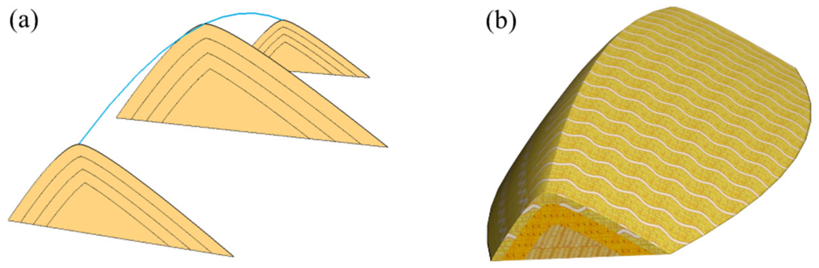
Examples of fold symbol models with different hinge lengths: (a) local morphology and (b) whole morphology.
Figure 19.
Examples of fold symbol models with different hinge lengths: (a) local morphology and (b) whole morphology.

Figure 20.
Fold structure modeling based on measured cross-section: (a) section of the Danaobo mountain syncline at Hanyang Peak of Mount Lu and (b) symbol model of the Danaobo mountain syncline.
Figure 20.
Fold structure modeling based on measured cross-section: (a) section of the Danaobo mountain syncline at Hanyang Peak of Mount Lu and (b) symbol model of the Danaobo mountain syncline.

Figure 21.
Construction process for the stratum boundaries of box folds.


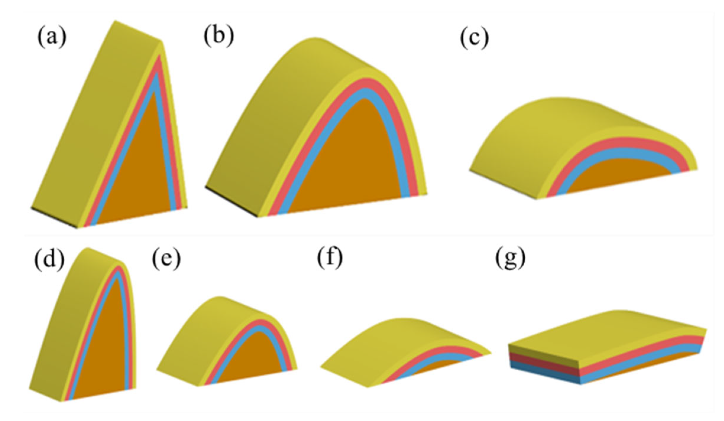
Table 1.
Main fold types and their characteristic parameters [41].
Table 1.
Main fold types and their characteristic parameters [41].
| Classification Basis | Fold Type | Morphological Characteristics | Parameters |
|---|---|---|---|
| Vertical section morphology | Upright fold | Axial surface is nearly vertical (80~90°); the inclination of the two limbs are opposite, and their dip angles are nearly equal. | Strike of axial surface; Strike of limbs; Interlimb angle |
| Oblique fold | Axial surface inclines; the inclination of two limbs tends to be opposite, and their dip angles are unequal. | ||
| Overturned fold | Axial surface inclines; the inclination of two limbs tends to be the same, and their dip angles are unequal. | ||
| Recumbent fold | Axial surface is nearly horizontal (1~10°), and one limb of the rock stratum overturns. | ||
| Circular fold | Folded surface is curved in a circular arc. | ||
| Chevron fold | Two limbs intersect straightly; the hinge zone is sharp; the interlimb angle is generally less than 30°. | ||
| Box fold | Two limbs are steep, the hinge zone is straight, and a pair of conjugate axial surfaces occurs. | ||
| Fan fold | Folded surface is fan-shaped, and both limbs are overturned. | ||
| Cross-section morphology | Gentle fold | Interlimb angle: 120~180° | Interlimb angle |
| Broad fold | Interlimb angle: 70~120° | ||
| Closed fold | Interlimb angle: 30~70° | ||
| Tight fold | Interlimb angle < 30° | ||
| Isoclinal fold | Interlimb angle ≈ 0°, the two limbs are parallel, and their occurrences are the same. | ||
| Longitudinal section morphology | Horizontal fold | Hinge is a horizontal line. | The occurrence of hinge; The occurrence of the axial surface. |
| Hinge fold | Hinge plunges. | ||
| Vertical fold | Both the hinge and the axial surface are nearly vertical (inclination angle: 80~90°). | ||
| Stratum thickness and morphological changes | Isopach fold | Stratum thickness is equal. | Curvature center, curvature radius, and thickness of each stratum. |
| Similar fold | One curvature radius, different curvature centers. | ||
| Harmonic fold | Bending morphology of each stratum is roughly the same. | ||
| Others | Including disharmonious folds, intestinal folds, and other folds whose strata morphology changes greatly. |
Table 2.
Modeling parameters of the fold structure.
| Parameter Type | Parameter Subdivision | Abbreviation | Unit | Parameter Description |
|---|---|---|---|---|
| Location parameters of cross-section | Center point of middle section | D | m | Determine the approximate position of the whole fold with the lower vertex |
| Fold width | d | m | Width range of the middle fold cross- section | |
| Distance between sections | dist | m | Control the overall length of folds | |
| Dip angle of hinge line | δ | ° | Angle between the hinge line and the horizontal line in the axial surface | |
| Strike of hinge line | μ | ° | Strikes of the hinge lines between the middle section and two end sections | |
| Dip angle of axial surface | γ | ° | Dip angles of the two end sections | |
| Morphological parameters of cross-section | Dip angle of axial surface | γ | ° | Dip angle of middle section |
| Dip angles of inflection points | α, β | ° | Dip angles of inflection points on both limbs of the reference stratum boundary in the middle section | |
| Interlimb angle | θ | ° | Interlimb angle of the middle section | |
| Morphological parameter | cur | - | Control the morphology of the hinge zone of each section | |
| Collection of strata thickness | Dep | m | Thickness of each fold stratum |
Table 3.
Affine transformation factor.
| Factor Name | Computing Formula | Variable Description |
|---|---|---|
| Magnification scale | δ is the front or back dip angle of the hinge in the location parameter, dist is the distance from the current section to the middle section, and h is the height from the actual upper vertex E to the lower vertex D in the middle section (Figure 5). | |
| Offset distance along X axis | μ is the front or back strike of the hinge in the location parameters, and dist is the distance from the current section to the middle section. | |
| Rotation angle | γ’ is the front or back section dip angle of the axial surface in location parameters, and γ is the dip angle of the axial surface in the middle section. |
Note: Please refer to Figure 3b for the relevant parameters.
Table 4.
Details of each experimental area.
| ID | Name | Fold Type | Source |
|---|---|---|---|
| 1 | Dayue Mountain in Mount Lu | Vertical horizontal anticline | [58] |
| 2 | Danaobo Mountain in Mount Lu | Oblique horizontal anticline | [59] |
| 3 | Fangdou Mountain in East Sichuan | Chevron fold | [60] |
| 4 | Scottish Highlands | Recumbent fold | [61] |
Table 5.
Modeling parameters of each experimental area.
| Type | Name | Unit | Dayue Mountain | Danaobo Mountain | Fangdou MOUNTAIN | Scottish Highlands |
|---|---|---|---|---|---|---|
| Location parameters | Center point of middle section | coordinate | (1000, 0, 0) | (1000, 0, 0) | (1000, 0, 0) | (1000, 0, 0) |
| Distance from front and back sections to middle section | m | 2000, 2000 | 2000, 2000 | 6000, 6000 | 2000, 2000 | |
| Fold width | m | 2000 | 2000 | 2000 | 1000 | |
| Front and back dip angles of hinge line | ° | −10, −10 | −5, −5 | 0, 0 | 0, 0 | |
| Front and back strikes of hinge line | ° | 0, 0 | −10, −5 | 0, 0 | 0, 0 | |
| Axial dip angles of front and back sections | ° | 80, 80 | 70, 70 | 95, 95 | 20, 20 | |
| Morphological parameters | Dip angles of axial surface | ° | 80 | 70 | 95 | 20 |
| Dip angles of inflection points | ° | 55, 35 | 40 | 120 | 150, 10 | |
| Morphological parameter | 0.8 | 0.4 | 0.95 | 0.6 | ||
| Collection of strata thickness | M | 50, 50, 50 | 50, 50, 50 | 30, 30, 30 | 40, 40, 40 | |
| Maximum rotation angle of distortion | ° | 0 | 0 | 0 | 30 |
Publisher’s Note: MDPI stays neutral with regard to jurisdictional claims in published maps and institutional affiliations. |
© 2022 by the authors. Licensee MDPI, Basel, Switzerland. This article is an open access article distributed under the terms and conditions of the Creative Commons Attribution (CC BY) license (https://creativecommons.org/licenses/by/4.0/).
Share and Cite
MDPI and ACS Style
Li, A.-B.; Chen, H.; Du, X.-F.; Sun, G.-K.; Liu, X.-Y. Parametric Modeling Method for 3D Symbols of Fold Structures. ISPRS Int. J. Geo-Inf. 2022, 11, 618. https://0-doi-org.brum.beds.ac.uk/10.3390/ijgi11120618
AMA Style
Li A-B, Chen H, Du X-F, Sun G-K, Liu X-Y. Parametric Modeling Method for 3D Symbols of Fold Structures. ISPRS International Journal of Geo-Information. 2022; 11(12):618. https://0-doi-org.brum.beds.ac.uk/10.3390/ijgi11120618
Chicago/Turabian StyleLi, An-Bo, Hao Chen, Xiao-Feng Du, Guo-Kai Sun, and Xian-Yu Liu. 2022. "Parametric Modeling Method for 3D Symbols of Fold Structures" ISPRS International Journal of Geo-Information 11, no. 12: 618. https://0-doi-org.brum.beds.ac.uk/10.3390/ijgi11120618
Note that from the first issue of 2016, this journal uses article numbers instead of page numbers. See further details here.