1. Introduction
Digital soil mapping (DSM), also known as predictive soil mapping or pedometric mapping, refers to the creation of digital maps that include spatial soil information, such as soil type or soil properties. These maps are created from the combination of multiple parameters (soil, climate, relief etc.) and usually depict the spatial distribution of soil phenomena along with relative information (e.g., estimation uncertainty).
DSM makes extensive use of geographic information systems (GIS), global positioning systems (GPS), remotely sensed spectral data, topographic data derived from digital elevation models (DEMs), predictive or inference models, and software for data analysis. To cope with the large amount of data used in DSM, semi-automated techniques and technologies are used to acquire, process, and visualize these data. Machine learning (ML) and artificial intelligence (AI) are some innovative state of the art technologies that are increasingly used in soil mapping and their uptake is transforming the way soil scientists produce their maps [
1]. ML that emerged in the 1990s as a tool for DSM [
2] is defined as the computer-assisted practice of using data-driven (and mostly non-linear) statistical models which resorts to a large amount of input data to learn a pattern and make a prediction [
1].
According to Leo Breiman [
3] two statistical modeling paradigms were distinguished: a data model and an algorithmic model. A data model is an abstract model that organizes elements of data and standardizes how they relate to one another and to the properties of real-world entities, whereas an algorithmic model is a model that uses mathematical algorithms based on the elements of data and estimates the parameters. One broadly used algorithm for that kind of model is Random Forests (RF). The RF is an ensemble learning method for classification, regression and other tasks that operates by constructing a multitude of decision trees at training time and is extensively used in DSM [
4]. For example, it provided the best results in estimating soil OM [
5], shortened the training time during the soil OM modeling process and improved the model’s accuracy and its predictive ability [
6]. Finally, according to John et al. [
7], RF was the best performing model among other ML algorithms such as artificial neural network (ANN), support vector machine (SVM), and cubist regression.
Most of the time, DSM products represent estimates of spatially distributed soil properties. These estimations comprise an element of uncertainty that is not evenly distributed over the area covered by DSM. If we quantify the uncertainty spatially explicitly, this information can be used to improve the quality of DSM by optimizing the sampling design [
8]. Wadoux et al. [
1] stated that while the (spatial) cross-validation results might show strong agreement between predicted and measured soil property or class and therefore validate a ML model with very high predictive abilities, an uncertainty quantification would show unrealistic predictions characterized by a large uncertainty. However, most ML methods RF included do not provide uncertainty estimates by default and only 30% of the recent soil studies in their literature review quantified the uncertainty associated with the prediction.
One ML method that intrinsically addresses the lack of uncertainty estimates is Quantile Regression Forests (QRF). The QRF is an extension of RF developed by Nicolai Meinshausen [
9] that provides non-parametric estimates of the median predicted value as well as prediction quantiles. It therefore allows spatially explicit non-parametric estimates of model uncertainty by providing information for the full conditional distribution of the response variable, and not only about the conditional mean [
10]. As a result, QRF can potentially combine the high accuracy of RF with the built-in uncertainty estimates. However, QRF is not broadly used in soil studies, despite its advantages.
Vaysse and Lagacherie [
11], for example, conducted an experiment in which they employed QRF in a temperate Mediterranean area with a comparable soil organic carbon (SOC) dataset in terms of areal extent, observation density, and distribution homogeneity. They claim that QRF outperforms RK when it comes to interpreting uncertainty patterns and is better suited than other modeling methods when spatial sampling is sparse. In Dharumarajan’s study [
12] the QRF model was used for the estimation of several important soil qualities of Northern Karnataka according to GlobalSoilMap criteria. The QRF model caught maximum variability for most of the soil parameters, and the predicted soil values were dependable with minimum errors. The QRF was also used for the production of global maps of soil properties explicitly highlighting the importance of quantitative and qualitative evaluation and uncertainty communication [
13]. Finally, in Veronesi’s study in 2019 [
14], RF and QRF generated the most reliable confidence intervals for predicting SOC. Even though this is potentially important for practical uses, the confidence intervals were also very wide, so they suggest that these intervals should be handled carefully.
In the current study, the prediction capability along with the uncertainty assessment capacity of the QRF is examined. The popular geostatistical methods of Ordinary Kriging (OK) and Kriging with External Drift (KED) were compared with the ML methods of RF and QRF, in the case of soil OM. Prediction maps of soil OM along with maps of uncertainties were also produced and presented. The study area that was chosen is in northern Greece, at the regional unit of Kastoria and next to the shore of Lake Orestiada. A total number of 414 samples of soil were collected in randomly sampled unique locations in autumn during a six-year period. GPS receivers were used to identify the sampling positions. A high-resolution Digital Elevation Model (DEM) was used to derive topographic products such as aspect, slope, altitude etc. along with Sentinel-2 imagery, for each year from our study period, to produce Normalized Difference Vegetation Index (NDVI) and Normalized Difference Water Index (NDWI) that were used as input data. Finally, the effect of the above-mentioned covariates to the prediction of soil OM was assessed based on the importance score of the applied machine learning methods.
2. Materials and Methods
2.1. Area of Study and Soil Sampling
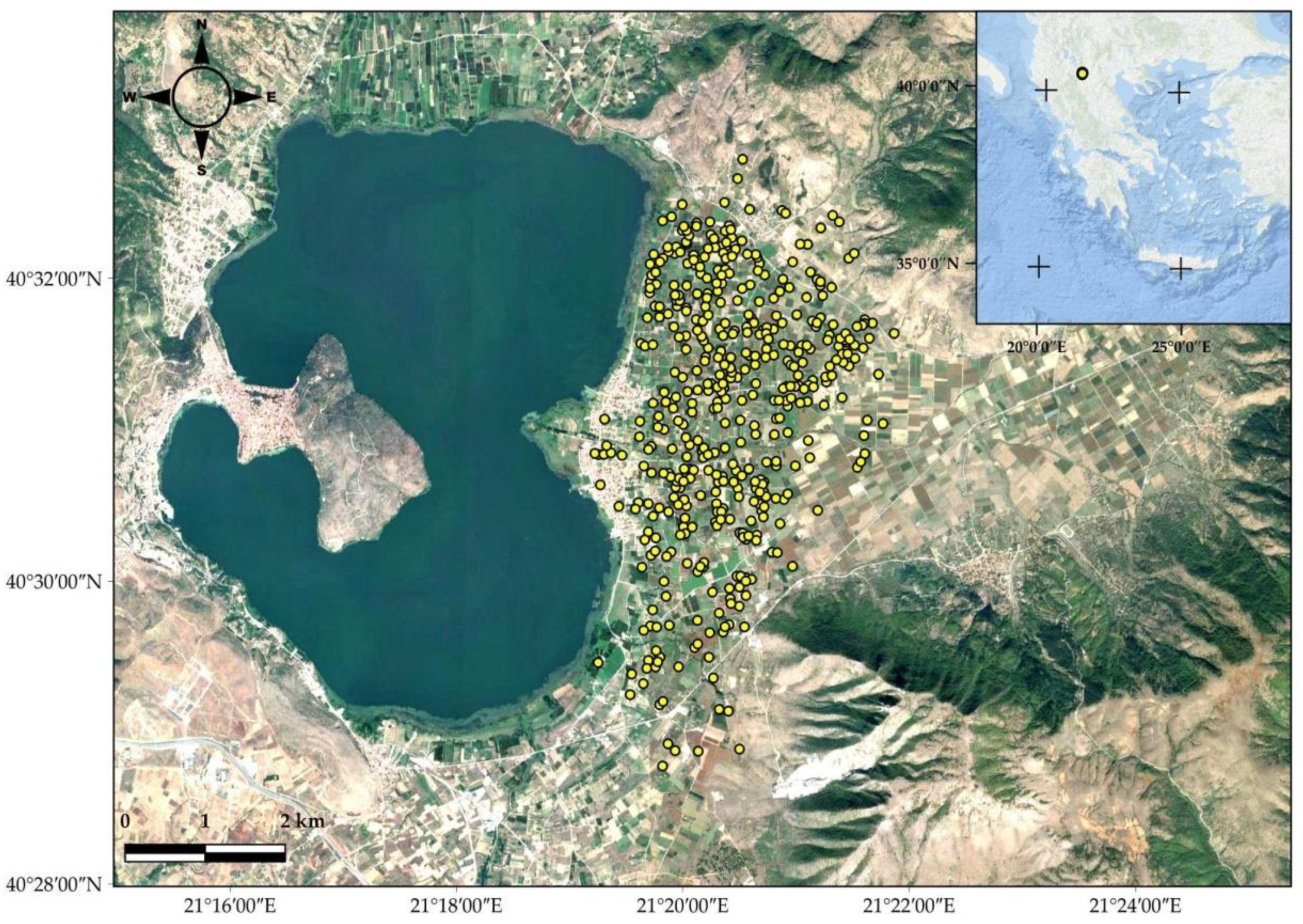
The study area was chosen in northern Greece, near the shore of Lake Orestiada, in the regional unit of Kastoria (
Figure 1). Its coordinates in the World Geodetic System of 1984 (WGS84) include the area between 40°28′42.41″ N and 40°32′35.61″ N latitudes and longitudes of 21°19′4.01″ E and 21°23′8.18″ E longitudes.
While the region of interest is flat, the mean altitude is around 640 m above sea level, ranging from 620 m near the lake to 700 m further north. The climate is temperate and often warm, with harsh winters that frequently keep the temperature below zero throughout the day. The average annual temperature is 11.5 °C, with 636 mm of precipitation. Summers are hot and dry, with a relative humidity of 50% to 55%. Apple trees and beans are the primary agricultural crops.
During a six-year period, a total of 414 soil samples were collected in randomly sampled distinct places around the study area (2012 to 2019). A total of 30 cm of top soil was gathered during late fall season (around end of November). The sampling positions were determined using Global Positioning System (GPS) devices. The minimum distance between two sampling places varies between 60 and 480 m, with an average of 90 m.
2.2. Soil, Environmental and Satellite Covariates
In this study, soil variables, environmental variables and satellite images were selected (
Table 1) as potential inputs in the models. Regarding soil covariates, the 414 soil samples that were collected from the area were analyzed for Clay (C) with soil hydrometer (Bouyoucos) method [
15], Magnesium (Mg) with ammonium acetate method and Zinc (Zn) with DTPA method [
16]. Moreover, an organic matter (OM) analysis (wet oxidation method) from the same locations was conducted, to calibrate the models and to assess the prediction results. In more detail, during the soil sampling procedure, a composite soil sample consisting of several sub-samples up to a depth of 30 cm was obtained from each field parcel and the soil samples were dried and analyzed in the laboratory of the Soil and Water Resources Institute in Thessaloniki, Greece.
The environmental covariates were derived from the second version of the Advanced Spaceborne Thermal Emission Radiometer-Global Digital Elevation Model version 2 (ASTER GDEM2). The release of the ASTER GDEM2 has enriched the availability of free-of-charge DEM sources, which are especially useful for developing countries, and prompted users to assess its quality and accuracy [
17]. The ASTER GDEM2 is consisted of 1° × 1° tiles (30 m resolution) in the World Geodetic System 1984 (WGS84), that was reprojected to Greek Geodetic Reference System 1987 (GGRS87) for this study [
18].
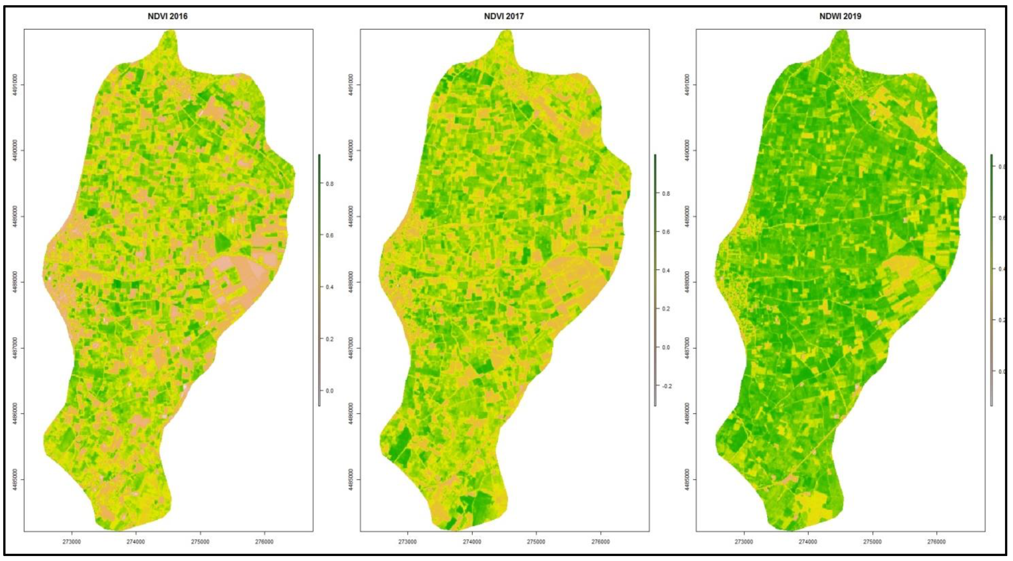
Moreover, satellite indices were derived from Sentinel-2 imagery. More specifically Normalized Difference Vegetation Index (NDVI) and Normalized Difference Water Index (NDWI) from 2016 to 2019 were collected at approximately the same time period that the soil data were collected (end of November). The well known and widely used NDVI is a simple, but effective index for quantifying green vegetation. Red light is actively absorbed by healthy plants, while near infrared is reflected. To determine the state of a plant’s health, we must compare the values of red and infrared light absorption and reflection [
7,
19]. The NDWI is a vegetation index sensitive to the water content of vegetation and is complementary to the NDVI. High NDWI values indicate a high plant water content and a high plant fraction coating. Low vegetation content and cover with low vegetation correspond to low NDWI values. The NDWI rate will drop during times of water stress [
20].
2.3. Data Preparation and Assessment
Initially, the topographic data and satellite indices along with the soil analysis data were combined and spatially overlayed on the sampling locations. The overall dataset was assessed for outliers and missing values. From the initial 414 points, 403 points remained at the end that were used as inputs for the models in the study.
From the full set of variables, only a subset was used in the study. The variables were eliminated using Akaike Information Criteria (stepAIC) technique and Principal Component Analysis (PCA) and were also assessed for multicollinearity. The remaining variables were C, OM, ZN, MG, Vdepth, Altitude, NDVI_2016, NDVI_2017, and NDWI_2019 (
Table 2).
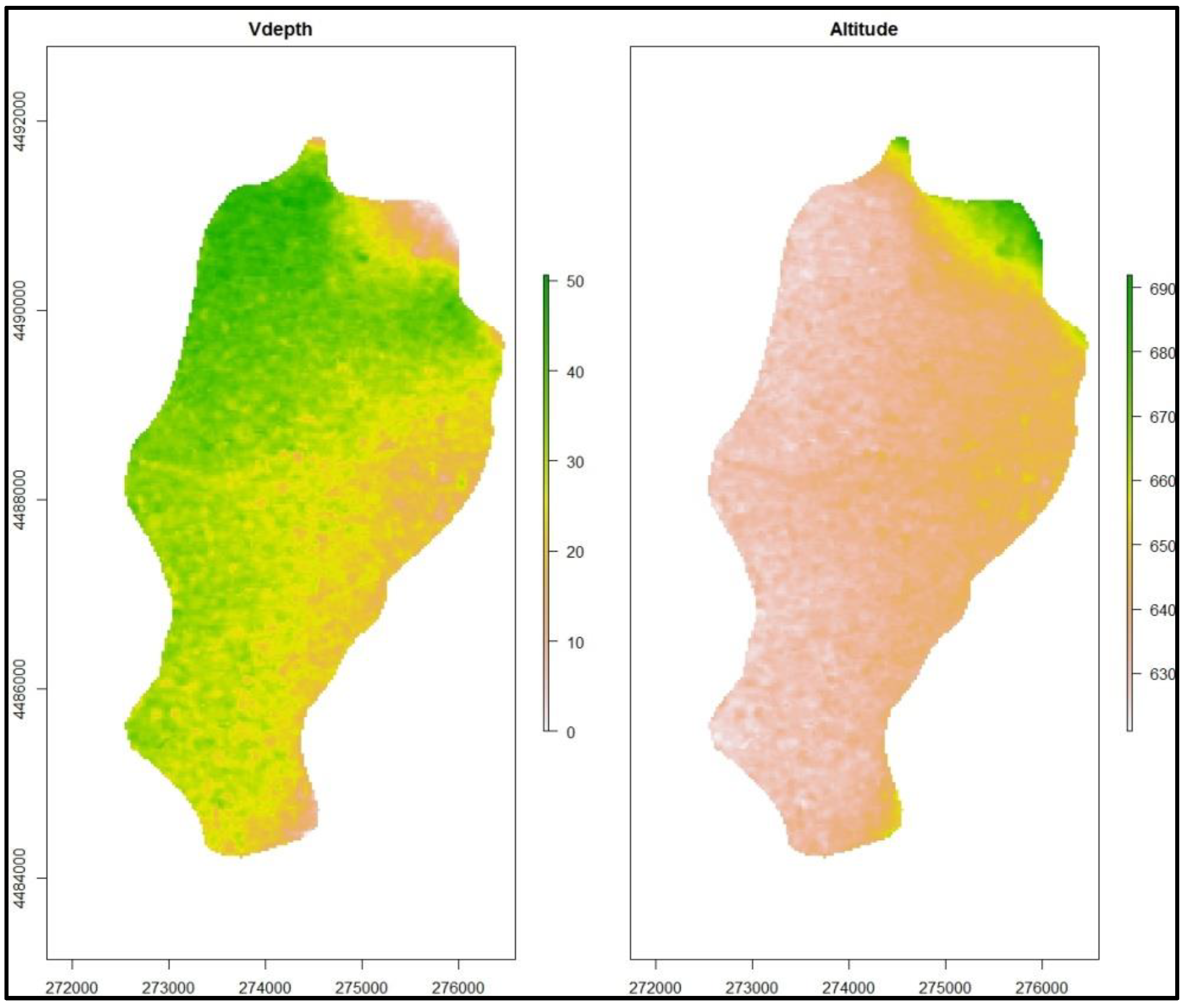
The maps of the spatial distributions of the environmental covariates that were derived from ASTER GDEM2 and were used in the study (Vdepth and Altitude), are presented next (
Figure 2).
The maps of the satellite covariates that were used in the study (NDVI_2016, NDVI_2017, and NDWI_2019) are the following (
Figure 3).
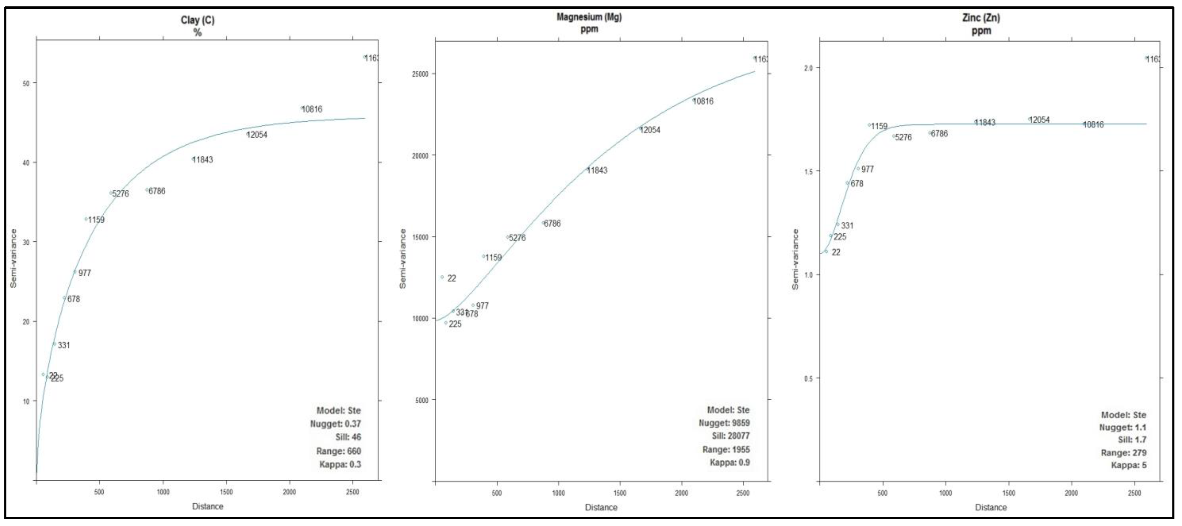
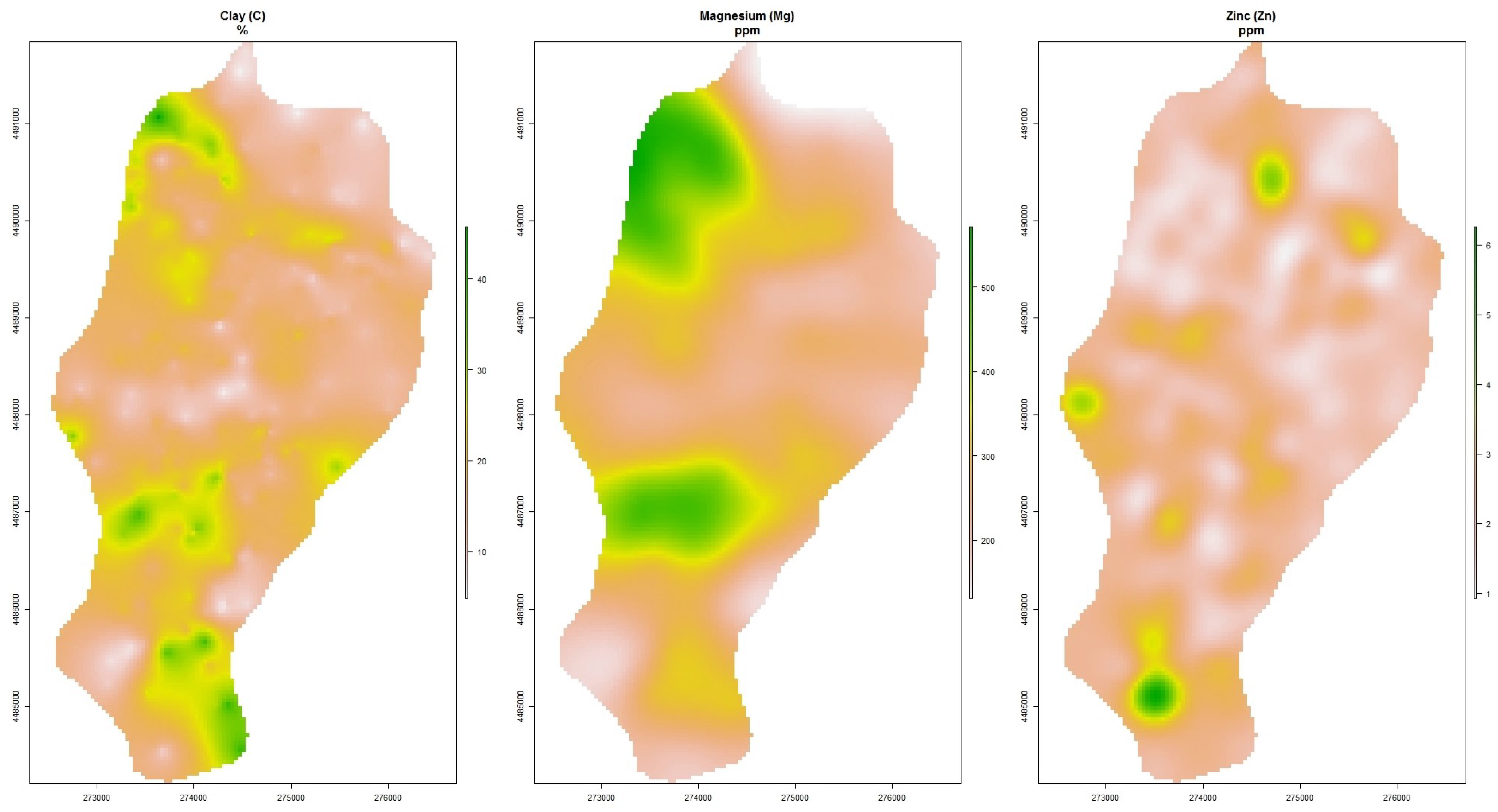
Finally, the soil covariates (C, MG, ZN) were interpolated from the known point locations of the full dataset with the use of OK and their spatial distribution for the overall study area was estimated (
Figure 4).
For all the soil parameters, the Matern semivariogram model with M. Stein’s parameterization (Ste) was applied as the fitted model using gstat’s default parameters. Regarding C, its range was 660 m and exhibited a strong spatial dependence with a nugget to sill ratio of 0.8% [
21]. The Mg had a range of 1955 m with strong spatial dependence (nugget to sill 3.5%) whereas Zn had a range of 279 m with moderate spatial dependence with a nugget to sill close to 65%.
The produced kriging maps from the soil covariates were used for the estimation of soil OM in the area by the models of the current study (KED, RF, QRF) (
Figure 5).
2.4. Ordinary Kriging (OK) and Kriging with External Drift (KED)
Ordinary Kriging is a type of kriging in which the values’ weights sum to one. It is linear because its estimates are a linear combination of the available data. It is also unbiased because it attempts to keep the mean residual to be zero and it tries to minimize the residual variance [
22]. The OK implicitly evaluates the mean in a moving neighborhood with local second-order stationarity and its variance is equal to the sum of the simple kriging variance (assuming a known mean) plus the variance due to uncertainty about the true mean value [
23].
Universal kriging (UK), Kriging with External Drift and Regression-Kriging (RK) belong to the group of the so-called ‘hybrid’ [
24], i.e., non-stationary geo-statistical methods [
23]. In classical geostatistics, spatial prediction for non-stationary processes is accomplished by taking into account a spatial trend (also known as “drift”) that is either modeled solely as a function of the coordinates (in UK) or defined “externally” through some auxiliary variables (in KED) [
25].
KED solves kriging weights by extending the covariance matrix with auxiliary variables so that the universality conditions are integrated into the kriging system; here, the difficulty is obtaining satisfactory residual variogram in the presence of drift [
26].
The implementations of both OK and KED in the current study was done with the gstat package in R.
2.5. Random Forests (RF) and Quantile Regression Forests (QRF)
The idea of developing the RF method is based on the combination of the Bagging and Random Subspace Method, utilizing their advantages and compensating their disadvantages, with impressive results [
3,
27].
According to Breiman (2001) [
3], in the case of classification, “A random forest is a classifier consisting of a collection of tree-structured classifiers {h(x, Θk), k = 1, …} where the {Θk} are independent identically distributed random vectors and each tree casts a unit vote for the most popular class at input x”. In case of regression Breiman states that “...random forests for regression are formed by growing trees depending on a random vector Θ such that the tree predictor h(x, Θ) takes on numerical values as opposed to class labels. The output values are numerical, and we assume that the training set is independently drawn from the distribution of the random vector Y, X”.
The RF for regression is extensively used in DSM (e.g., [
28,
29,
30,
31,
32,
33]) with very positive results in the prediction of different soil parameters. More importantly though, it works equally well with skewed and normally distributed variables, without the need of statistical assumptions or restrictions that other methods demand. Therefore, it is easier and more straightforward to use. It just requires special attention in optimizing the hyperparameters to get the best results. One major drawback of some of the well-known ML methods (RF, ANN etc.) is their lack of intrinsic uncertainty estimation capabilities. So, apart from prediction maps, no prediction error variance can be estimated, contrary to classical geostatistics methods. The main reason for this is that most ML methods, RF included, provide only mean value predictions.
A possible solution to this deficiency came from Nicolai Meinshausen [
9], who generalized the standard RF to provide information for the full conditional distribution of the response variable, and not only about the conditional mean. This ML algorithm is called Quantile Regression Forests (QRF) and gives a non-parametric and accurate way of estimating conditional quantiles for high-dimensional predictor variables. The key difference between QRF and RF is as follows: for each node in each tree, RF keeps only the mean of the observations that fall into this node and neglect all other information. In contrast, QRF keeps the values of all observations in this node, not just their mean, and assesses the conditional distribution based on this information.
In the current study, the ranger package in R language was used to implement the ML models. Ranger is a rapid implementation of RF or recursive partitioning that is especially well suited for high-dimensional data.
The assessment of the optimal hyperparameters of a ML model is a crucial step for the estimation of the best ML models for each specific use case. The ideal hyperparameter settings have a direct impact on the model’s performance. Although there are various automatic optimization methods, their strengths and drawbacks change when applied to different types of situations [
34]. In the current study, the random search method was performed (a 10 k-fold with 3 repeats), in which random combinations of parameters were employed from a range of values and used as hyperparameters. The ML model with the set of parameters that gave the highest accuracy was considered to be the best and used for prediction. The overall dataset (403 samples) was split in two distinct datasets: the training dataset (70% of the data) that was used for estimating the models hyperparameters and the testing dataset (30% of the data) that was used for assessing the different models. The specific hyperparameters for RF that were optimized are presented in
Table 3.
2.6. Uncertainty
The DSM products represent estimates of spatially distributed soil properties. These estimations comprise an element of uncertainty that is not evenly distributed over the area covered by DSM [
8]. These flaws are being addressed by combining soil data at sites with spatially exhaustive environmental factors using quantitative models (e.g., [
35,
36,
37]) DSM products are repeatable and enable continuous data display due to their quantitative nature. Models can also be updated for multiple reasons, and uncertainty can be measured [
38,
39].
Measurements, digitisation, data input, interpretation, categorization, generalisation, and interpolation are all common sources of mistake [
40]. Modeling bias, parameterization, or even measurement mistakes connected with the input data can all cause uncertainty in digital soil maps [
41]. Nelson et al. [
42] recommends doing an error budget to assess the contribution of each error using a combination of geostatistical and Monte-Carlo simulations to gain a better understanding of uncertainty. The distinction between model error and spatially explicit uncertainty must also be considered [
43]. The average squared difference between the estimated value and the actual value is known as model error, which is frequently assessed as the mean square error (MSE) [
44,
45]. However, spatially explicit uncertainty, often known as “local error”, refers to the quantification of model output prediction intervals (e.g., [
11,
44,
46]).
The prediction is linked to an explicit measure of the uncertainty. In many circumstances, such as in a decision-making process, it is just as important to quantify prediction uncertainty as it is to make the prediction itself, thus uncertainty maps are necessary (e.g., [
47,
48]). In DSM, uncertainty analysis is crucial in deciding whether the predicted soil map is dependable enough to be applied in agricultural production systems or decision-making. Uncertainty analysis also involves acknowledging the model’s limitations, which is a step toward model interpretability [
1]. As Heuvelink [
49] states, we are very interested in prediction intervals in soil mapping, i.e., the range that is likely to contain the value yet to be measured. However, a very small amount of DSM studies estimate uncertainty. According to Wadoux [
1], only around 30% of the studies presented in their paper quantified the prediction’s uncertainty.
In the current study the uncertainty was estimated for only three out of four methods: OK, KED, QRF. The RF does not provide uncertainty estimation capabilities per se. The geostatistical methods of OK and KED provide by default the variance that it was used for the uncertainty assessment. Mainly, the standard deviation was calculated and its range was depicted in the maps. For the QRF the range was defined as one standard deviation above and below the median value. This range was used to create the uncertainty map of the study area
2.7. Error Assessment
Different metrics (
Table 4) were employed to estimate model performance based on the difference between the observations and the predictions at the testing data set.
The root mean square error (RMSE) and the mean absolute error (MAE) were estimated, based on the measured value and its prediction in locations of the samples (Equations (1) and (2)). The MAE is the average of the absolute values of the differences between the forecast and the corresponding observation over the verification sample. Since the MAE is a linear score, all individual differences are weighted equally in the average. The RMSE is a quadratic scoring rule that calculates the average magnitude of the error. Because errors are squared before being averaged, the RMSE gives large errors a relatively high weight. As a result, the RMSE is most useful when large errors are especially undesirable. The MAE and RMSE both have a range of 0 to ∞. They’re negative scores, thus the lower the number, the better. The coefficient of determination (R2) (Equation (3)) represents a model’s ability to predict or explain an outcome. The R2 indicates the percentage of variance in the predicted variable and the measured variable where SSE is the sum of squares of errors and SSTO the total sum of squares. The coefficient of determination ranges from 0 to 1, where in 0 (zero) no variation is explained by the model and in 1 (one) all variation is explained by the model. A high R2 value, in general, implies that the model is a good fit for the data, though fit interpretations vary depending on the context of analysis. Finally, the mean bias error (MBE) was used as a measurement of the bias estimation of the models (Equation (4)).
2.8. Software
For the statistical analysis of the current study, the R (version 4.0.3) statistical software and the caret package were used [
50]. Also, the ranger package [
51] was utilized for RF and QRF. The geostatistics were implemented with the gstat package [
52]. Finally, the Saga-GIS software (
https://saga-gis.sourceforge.io/en/index.html (accessed on 18 November 2021)) was used for the environmental indices.
3. Results
3.1. Semivariograms and Fitting Parameters of OK and KED
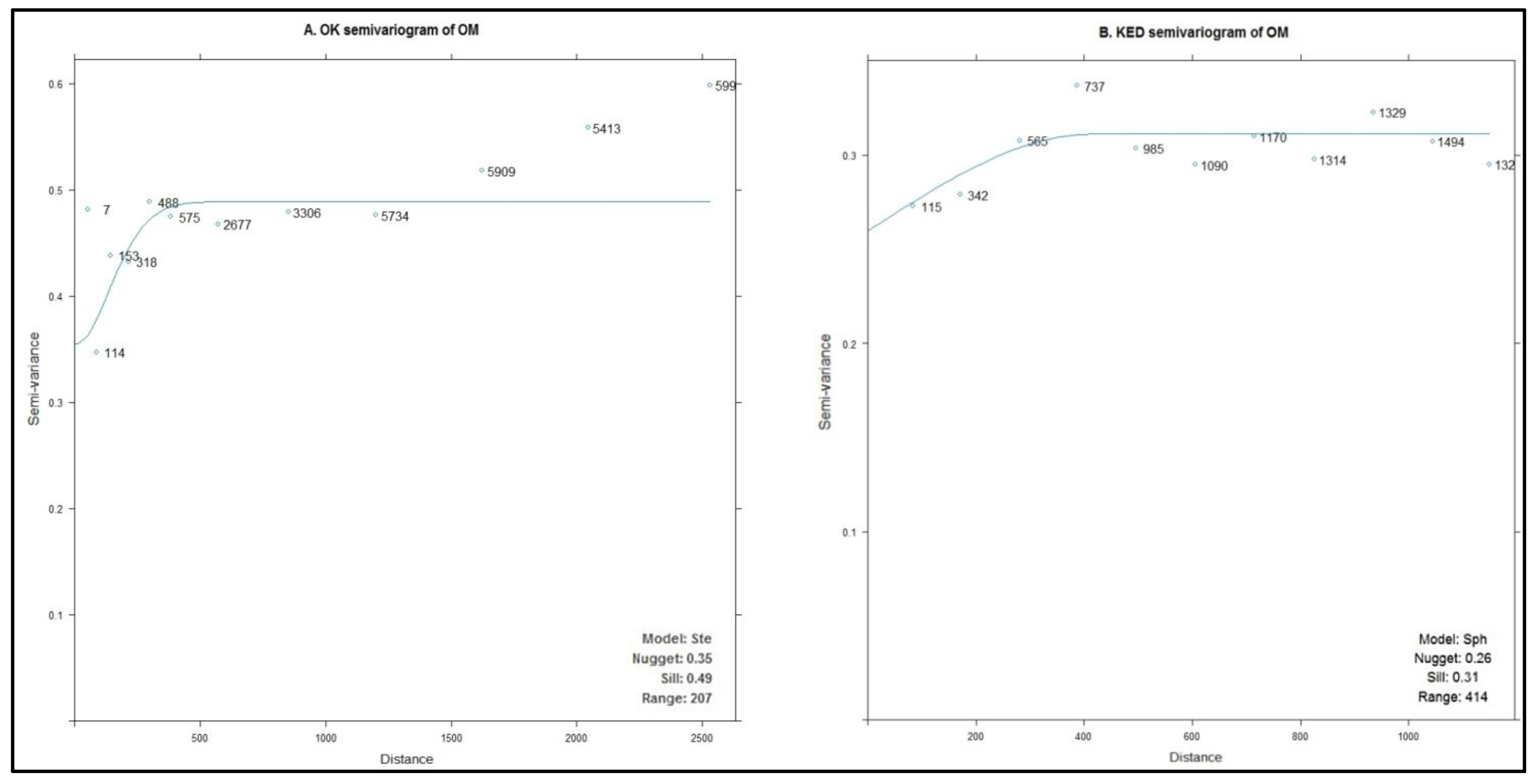
Initially, OK and KED were implemented using the training dataset for the prediction of the soil OM in the study area. In the case of OK, based on the empirical semivariogram, the Matern semivariogram model with M. Stein’s parameterization (Ste) was fitted (
Figure 6) using the weighted least square fit of gstat package. The range was 207 m with a nugget at 0.35 and sill at 0.49. There was a moderate spatial dependence based on the nugget to sill ratio (71%).
Regarding KED, the spherical model was used for fitting with the default method of gstat based on weighted least squares fit. The range was at 414 m, double than the OK range. In this case there was a weak spatial dependence with a nugget to total sill ratio of 83%.
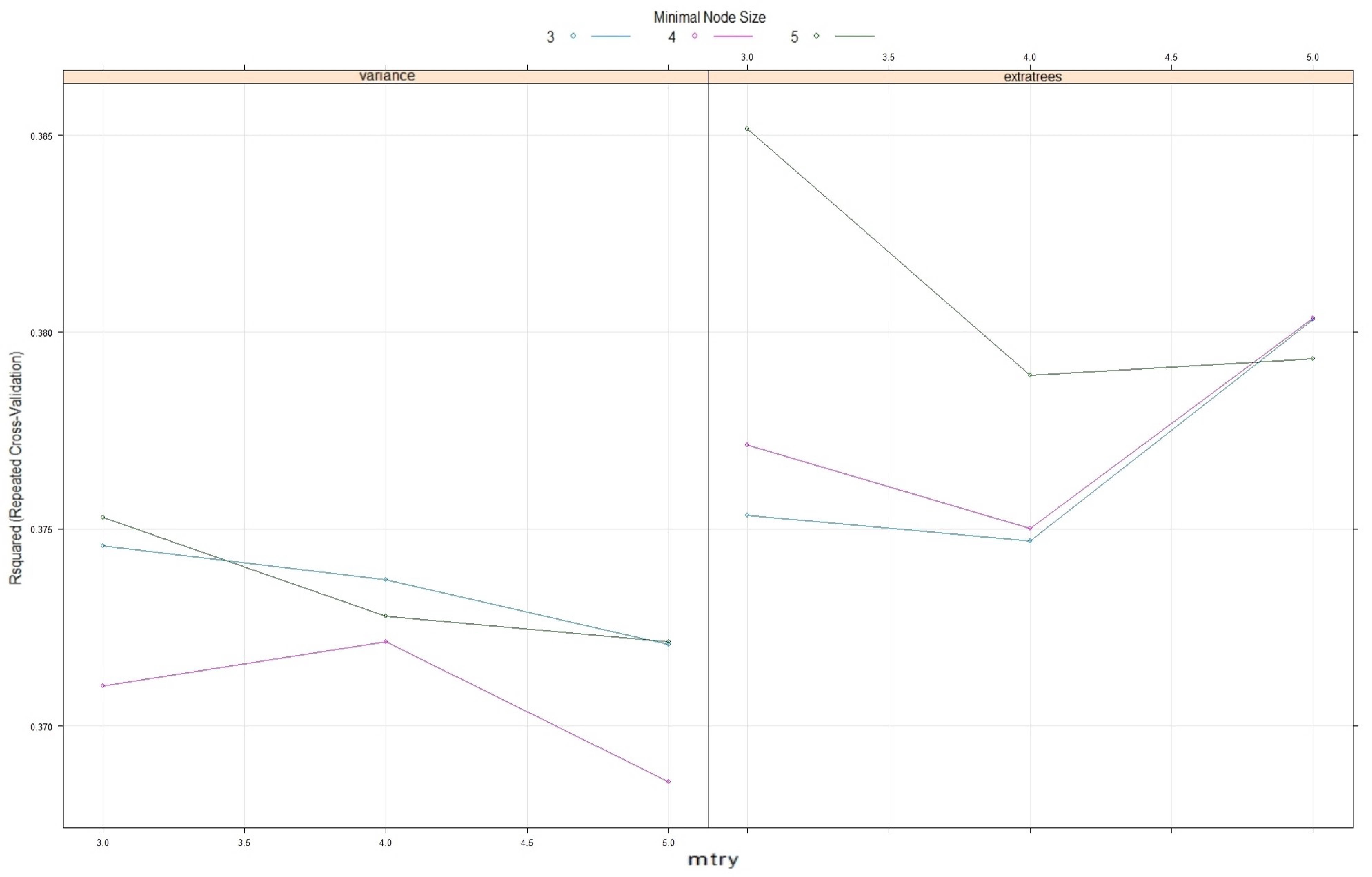
3.2. RF and QRF Hyperparameters’ Optimization Results
As it is already stated (
Section 2.5), ML models need the assessment of their optimal hyperparameters in order to provide the best prediction results. In the case of RF and QRF as defined by the ranger library, four hyperparameters need to be estimated (
Table 3). An iterative process (trial and error) was used with the random search optimization method, where different random values of these parameters were introduced from a range of values. The R
2 of the ML models was assessed using a 10-fold cross-validation method that was repeated 3 times in the training data set (
Figure 7). The hyperparameters that returned the highest R
2 were finally chosen (
Table 5).
For the splitrule hyperparameter, only “variance”and “extratrees” methods were used due to unrecoverable errors from “maxstat” and “beta” values.
The specific optimal hyperparameters were introduced in the RF and QRF models and used to estimate their prediction capabilities on the testing dataset.
3.3. Feature Importance of the ML Models
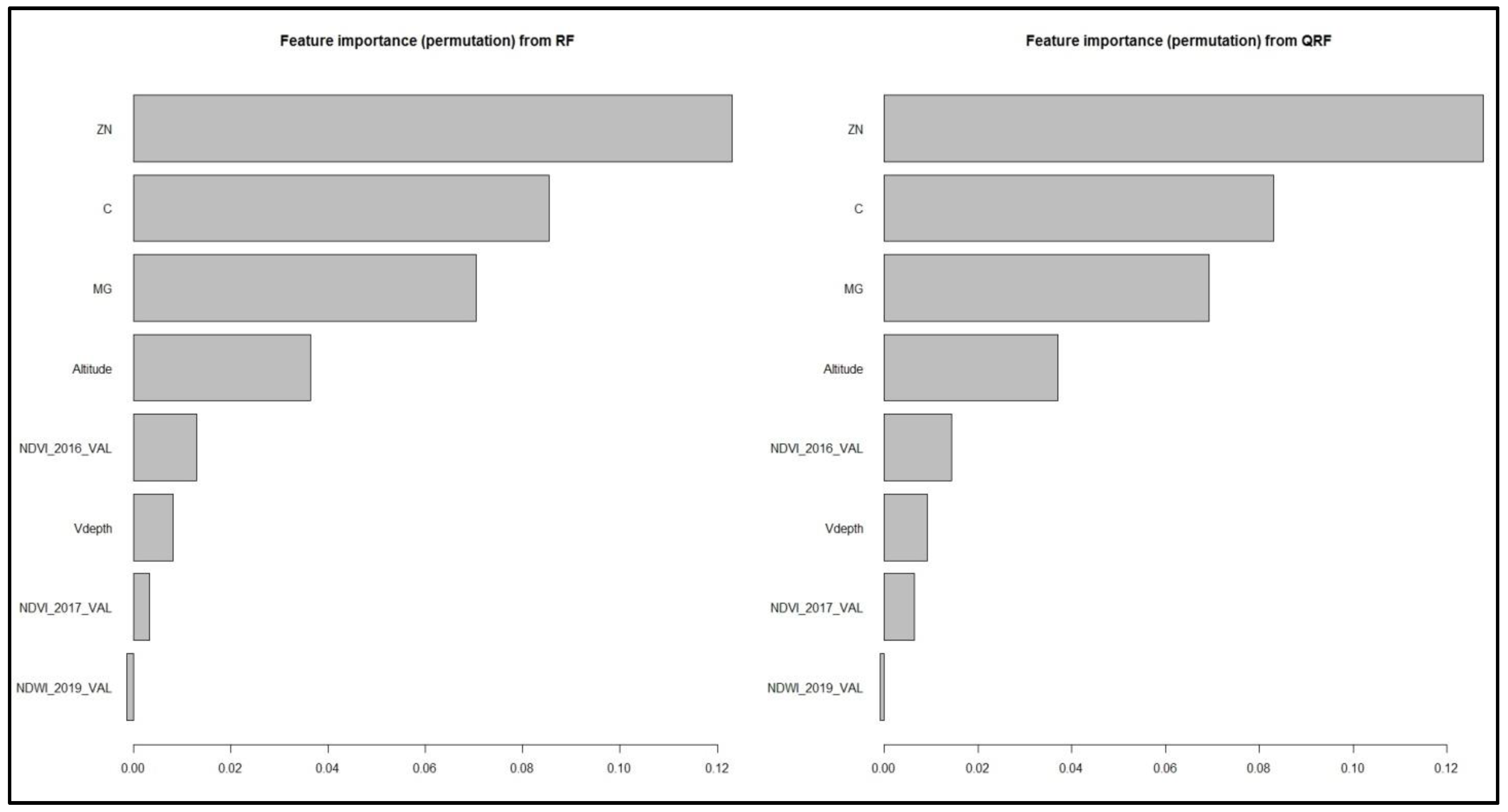
The feature importance of the RF and QRF was estimated (
Figure 8) with the permutation technique [
3], that is defined as the decrease in the model score when a single feature value is randomly shuffled. A feature is “important” if shuffling its values increases the model error (strong effect on the prediction) and “unimportant” if shuffling its values leaves the model error unchanged (low or no effect on the prediction).
Regarding the importance scores, both RF and QRF concede that the soil covariates exhibited the highest importance, something that was expected due to comparable findings of a previous study [
28] in a nearby area. In the current study specifically, Zn had the highest score with C second and Mg third. The Altitude from the topographic indices was next, along with the NDVI of 2016 and Vdepth. The last positions were occupied by NDVI of 2017 and NDWI of 2019.
3.4. Prediction Results
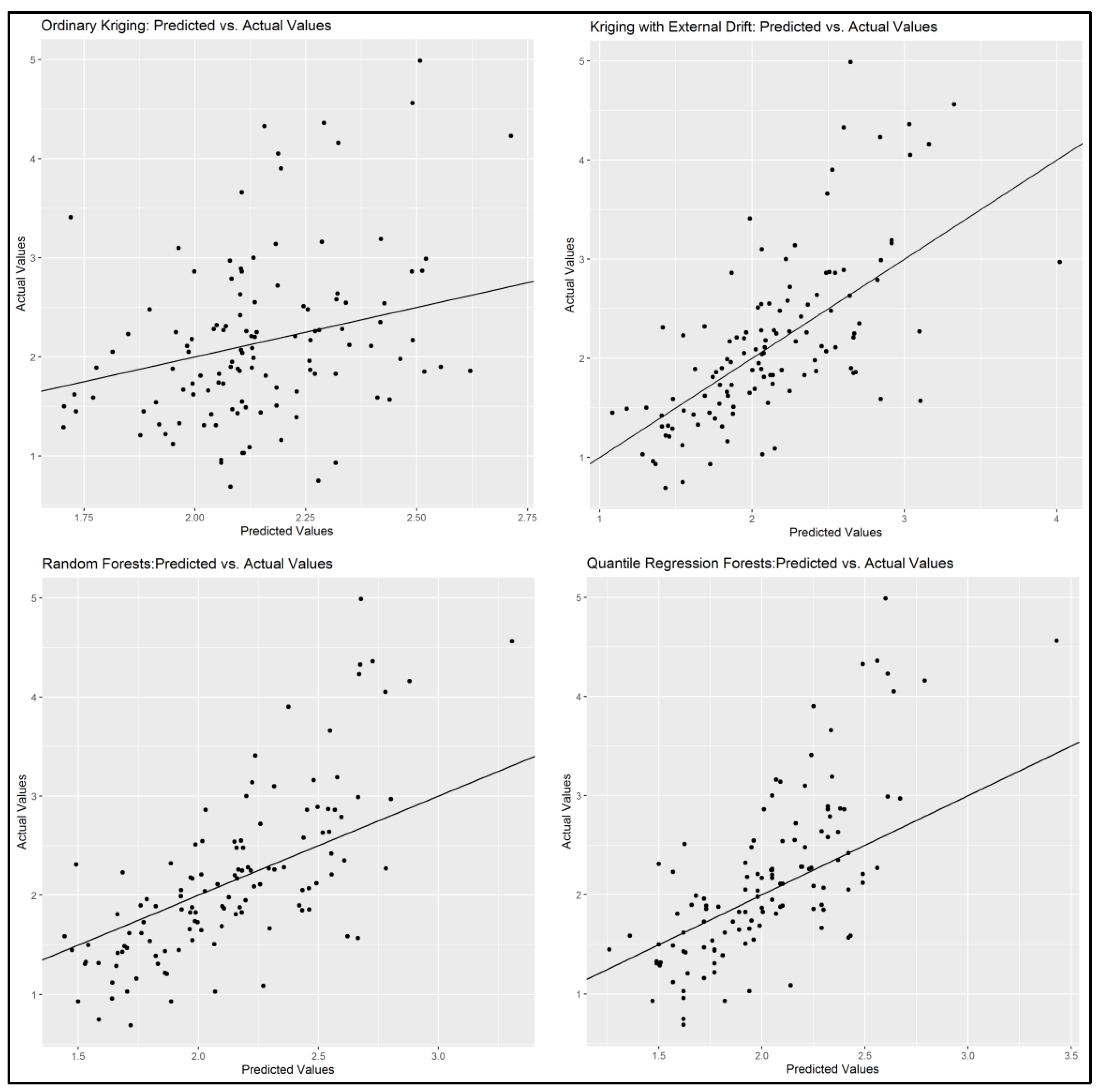
The dataset was partitioned into two random but spatially balanced sets of 70% for training the models and 30% for testing. The difference between the observations of the soil OM and their predictions in the testing data set was used to assess the prediction accuracy of the different models and they are presented in
Table 6 and
Figure 9.
As it is presented in the results (
Table 6), OK was the least accurate model with very low R
2 (0.127) and high RMSE and MAE, something that was expected due to its lack of capacity to incorporate auxiliary information. The OK prediction capability is based only on the variable’s (OM) spatial autocorrelation, hence the poor current results. It presented the smaller bias though based on the MBE (−0.002).
The KED combines the predictive capabilities of the trend that is based on the auxiliary variables, along with the kriging interpolation. Therefore, the results are decent, with low RMSE (0.618) and MAE (0.455) that are very close to RF and even slightly better than QRF. However, the coefficient of determination (0.452) is much worse than the ML methods. The bias was also small close to zero (−0.022), however higher than the OK.
The ML models exhibited higher prediction capabilities than geostatistical models. More specifically, the best results were achieved by the RF. Especially its R2 was the highest (0.538) among the models with an improvement of around 20% from KED. Regarding RMSE and MAE, RF’s results were best with the lowest values overall. The model bias was low (−0.020) close to KED’s value.
The QRF model also exhibited very good prediction capabilities with high R2 (0.532) very close to RF and quite low RMSE and MAE, close to RF and KED. The MBE was higher than the other models (−0.046), however still low and close to zero. Thus, RF and QRF can both be used interchangeably for predicting soil OM with similar results in the current study.
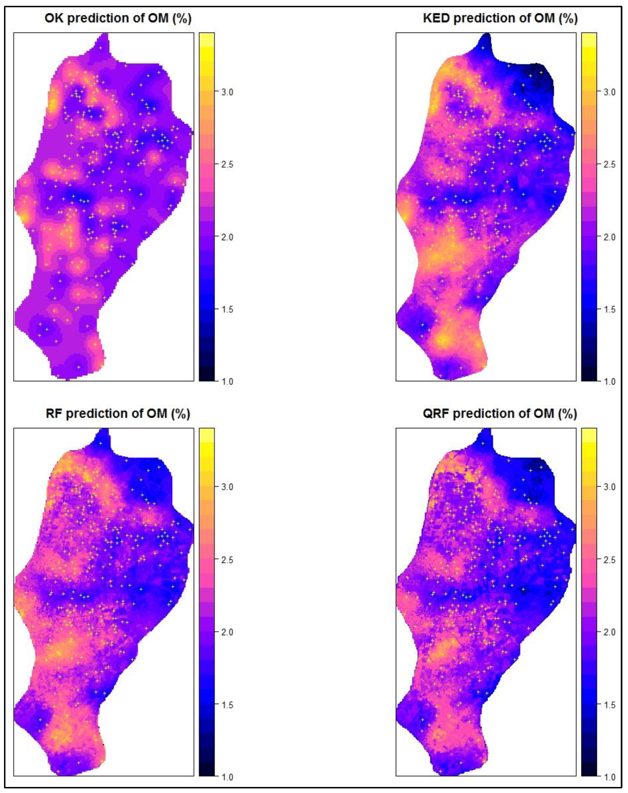
3.5. Maps of Prediction and Uncertainty
Next, two sets of maps were produced from the different models of the current study. The first set consists of four prediction maps that present the spatial distribution of soil OM in the area, one for each method: OK, KED, RF and QRF (
Figure 10). The second set of maps consist of three maps with OK, KED and QRF methods that depict the spatial distribution of prediction’s uncertainty in the area (
Figure 11). In this case the RF was not used due to its lack of uncertainty capabilities.
The prediction map of OK exhibited interpolation results with prediction patterns that are relatively uniform all over the study area. The main reason for this is that OK is based solely on the spatial autocorrelation of OM using global model parameters that smooths the results. The KED model produces a map that changes more abruptly due to its covariates’ effect, leading to multiple areas with higher and lower local values than the OK. Regarding ML methods (RF, QRF) their maps had even more contrast than the OK and KED, due to their capability of producing patterns that match data as much as possible by better fitting to the dataset. Among them, the QRF seem to present slightly more abrupt patterns than RF with areas with slightly lower and higher values.
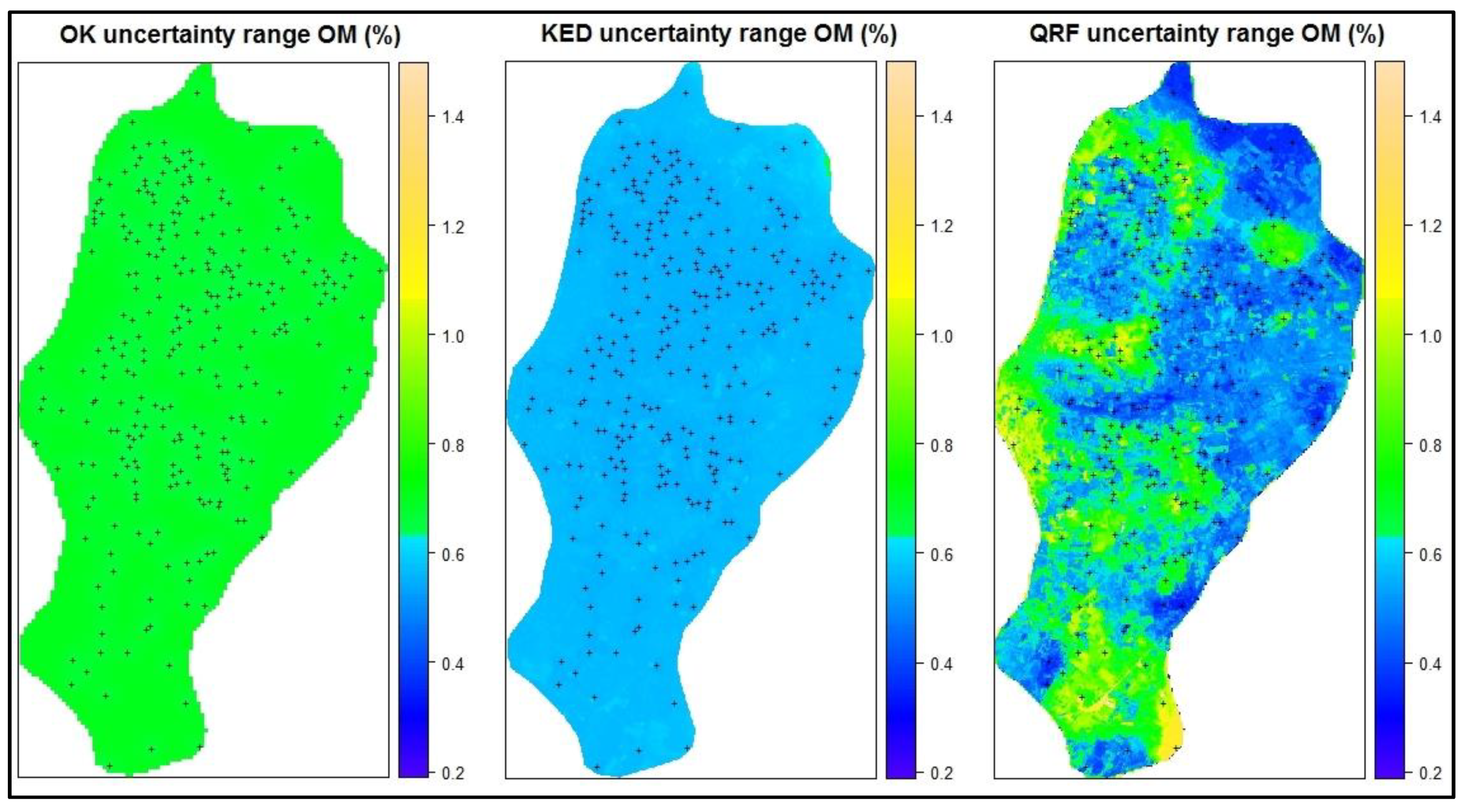
As it was already mentioned, apart from the prediction results, prediction’s uncertainty is a crucial parameter that needs to be estimated in the different locations of the study area. In the current study the uncertainty maps were calculated for only the 3 out of 4 methods. The RF does not support uncertainty estimation. The OK and KED intrinsically provide the error variance by which the standard deviation was calculated and its range was presented in the maps. For QRF the range was defined as one standard deviation above and below the median and it was used to create the uncertainty map of the study area (
Figure 11).
Based on the uncertainty maps, it is obvious that OK has a smooth and equally distributed uncertainty range in the area with a mean value approximately at 0.8%. So, in each location the real OM value is approximately ±0.4% above or below the predicted value.
The KED uncertainty map has an overall lower uncertainty range than the OK (around 0.6%), that is almost equally distributed in the overall study area, similarly to OK. There are some slightly increased range values in the northern-west area along with some small patches in between (lighter blue areas) due to the covariates minor effect on the uncertainty results.
In the case of QRF, the uncertainty map is more diversified than the previous ones. There are distinct regions of very low uncertainty like the one in the north or in the center of the area (with dark blue color) and regions of higher uncertainty like the ones in the south or close to the lake (with yellow color). This clear depiction of the uncertainty in a local scale and the straightforward definition of possible uncertainty zones, is a major advantage over the geostatistical methods especially for decision support purposes.
4. Discussion
One of the core tasks in the DSM studies is the estimation and presentation of the spatial distribution of different soil variables in the study area using different interpolation methods. Apart from that though, estimating and presenting the uncertainty of these interpolation methods are equally important in order to assess the overall work, something that is lacking in some of the recent DSM studies, especially the ones that are based on ML.
The ML methods are increasingly used in DSM, based on their outstanding prediction capabilities that outperforms the classic geostatistical methods, without the drawbacks of statistical assumptions and the restrictions of other methods. However, most of them do not have intrinsic uncertainty estimation capabilities. The RF is a very promising ML method used in multiple DSM studies that nevertheless lacks built-in uncertainty estimation capacity. An interesting alternative is QRF that seems to provide advanced prediction capabilities similar to RF along with innate uncertainty estimation metrics.
In the current paper, it was confirmed that QRF exhibited outstanding results at predicting soil OM in the study area, very close to RF method. Especially R2 was much higher than the geostatistical methods, something that signifies that more variation is explained by the specific model. Moreover, its uncertainty capabilities as presented in the uncertainty maps, shows that it can also provide a very efficient estimation of the uncertainty in the study area. Uncertainty map with QRF exhibit stronger contrast compared to uncertainty maps of OK, and KED, with distinct representation of the local variation of the uncertainty such as small regions with higher or lower uncertainty. Based on this map it is very easy for a user to define clusters of uncertainty zones and categorize its effect locally. This is a real significant advantage, especially for decision support purposes in which users are interested not only in the prediction accuracy but also in the variation of the error range in different parts of the area.


