Spectral Index for Mapping Topsoil Organic Matter Content Based on ZY1-02D Satellite Hyperspectral Data in Jiangsu Province, China

Abstract

Estimation of soil organic matter content (SOMC) is essential for soil quality evaluation. Compared with traditional multispectral remote sensing for SOMC mapping, the distribution of SOMC in a certain area can be obtained quickly by using hyperspectral remote sensing data. The Advanced Hyper-Spectral Imager (AHSI) onboard the ZY1-02D satellite can simultaneously obtain spectral information in 166 bands from visible (400 nm) to shortwave infrared (2500 nm), providing an important data source for SOMC mapping. In this study, SOMC-related spectral indices (SIs) suitable for this satellite were analyzed and evaluated in Shuyang County, Jiangsu Province. A series of SIs were constructed for the bare soil and vegetation-covered (mainly rice crops and tree seedlings) areas by combining spectral transformations (such as reciprocal and square root) and dual-band index formulas (such as ratio and difference), respectively. The optimal SIs were determined based on Pearson’s correlation coefficient ($\rho$) and satellite data quality, and applied to SOMC level mapping and estimation. The results show that: (1) The SI with the highest $\rho$ in the bare soil area is the ratio index of original reflectance at 654 and 679 nm (OR-RI_(654,679)), whereas the SI in the vegetation area is the square root of the difference between the reciprocal reflectance at 551 and 1998 nm (V-RR-DSI_(551,1998)); (2) the spatial distribution trend of regional SOMC results obtained by linear regression models of OR-RI_(654,679) and V-RR-DSI_(551,1998) is consistent with the samples; (3) based on the optimal SIs, support vector machine and tree ensembles were used to predict the SOMC of bare soil and vegetation-covered areas of Shuyang County, respectively. The determination coefficient of the soil–vegetation combined prediction results is 0.775, the root mean square error is 3.72 g/kg, and the residual prediction deviation is 2.12. The results show that the proposed SIs for ZY1-02D satellite hyperspectral data are of great potential for SOMC mapping.

1. Introduction

Soil organic matter (SOM) is essential for soil nutrients and a key indicator for evaluating soil environment [1] and food security [2]. It provides nutrients for crop growth [3,4,5] and plays a vital role in soil formation, conservation, environmental protection, and sustainable development of agriculture and forestry [2]. Changes in the abundance and properties of SOM profoundly impact many processes in the soil ecosystem. Therefore, SOM monitoring is necessary to keep track of soil environmental conditions. Traditional estimation of soil organic matter content (SOMC) mainly relies on collecting a large number of soil samples and laboratory chemical analysis. This method is relatively accurate, but the alteration of soil’s natural status and mass loss is inevitable during the sampling and measuring process [6]. It is also time consuming and laborious, and it is difficult to achieve large-scale investigation in a short time [7]. Soil proximal sensing methods can achieve non-destructive measurements, yet only soil properties at the sampling point can be obtained [8]. Therefore, it is challenging to obtain the spatial distribution of SOM at a regional scale [9].

Satellite remote sensing has the advantages of fast monitoring, wide coverage and low cost [9]. In particular, hyperspectral satellite data have rich spectral information, making it possible to predict the spatial distribution of SOMC on a large scale and with high accuracy [10]. The ZY1-02D satellite, launched in September 2019, carries an Advanced Hyperspectral Imager (AHSI) that can simultaneously acquire spectral information in 166 bands from the visible (400 nm) to the shortwave infrared (2500 nm) with a swath width of 60 km [11]. AHSI can obtain spectral details of the absorption features of SOM from hundreds of continuous narrow bands [10,12], making it an important data source for SOM mapping.

In recent years, many researchers have studied the monitoring of SOMC by satellite remote sensing. For example, Tiwari et al. [13] used artificial neural network (ANN) algorithms to model and map soil organic carbon (SOC) in New Delhi, India, based on EO1-Hyperion images. Emadi et al. [14] drew SOC in northern Iran using ANN, random forest (RF) and support vector machine (SVM) algorithms based on Landsat 8 and MODIS data. The Food and Agriculture Organization of the United Nations (FAO) offered [15] step-by-step guidance for developing 1 km grids for SOC stocks in the Soil Organic Carbon Mapping cookbook. Venter et al. [16] used satellite-driven high-resolution maps to map SOC stocks and trends over South Africa and the depth reached 30 cm. European Union’s Copernicus programme used the Sentinel satellite to estimate SOC in European croplands [17]. Endsley et al. [18] estimated a daily global carbon budget including surface (0–5cm depth) SOC with the SMAP Level 4 Carbon (L4C) product. However, satellite remote sensing can only be used to estimate the topsoil organic matter content, and the accurate assessment of the actual SOC quantity stored in other layers is still a huge challenge.

The absorption characteristics of soil spectral reflectance are mainly due to the overtones and combinations of fundamental vibrations caused by the stretching and bending of N-H, O-H and C-H groups [19]. The significant negative correlation between SOM and soil spectral reflectance is the foundation for predicting the spatial distribution of SOM [20]. In the bare soil area, researchers have proposed many different forms of soil spectral indices (SIs) to estimate SOMC. For example, Krishnan et al. [21] used the first derivative absorption rate index (FDAI), absorption ratio index I (ARI I) and absorption ratio index II (ARI II) to estimate the SOMC in Illinois, USA. Based on the absorption characteristics of soil biochemical components, Bartholomeus et al. [22] constructed multiple SIs that have strong correlations with SOC. Jin et al. [23] analyzed the correlations between the difference index (DI), ratio vegetation index (RI), normalized difference vegetation index (NDI) and SOMC. However, most of these indices were constructed based on laboratory soil spectra. Due to the difference between laboratory soil samples and field soils and the influence of the observation scale, it is challenging to obtain satisfying results when these indices are directly applied to satellite data.

In the vegetation-covered area, SOM plays a vital role in crop growth. For example, the humic acid in SOM is an essential source of SOC in the vegetation-covered area. Humic acid can stimulate plant growth and absorb colloidal cations [3,24,25]. Cellulose, lignin and other components of vegetation are usually affected by SOM, which leads to changes in the absorption characteristics of the vegetation canopy spectrum [26]. In the vegetation-covered area, according to this indirect interaction mechanism between SOM and vegetation canopy spectrum, researchers tried to relate SOMC with vegetation SIs that can indicate chlorophyll content, moisture and cellulose content. In previous studies, some vegetation SIs have been applied to evaluate SOMC, such as the normalized difference vegetation index (NDVI), enhanced vegetation index (EVI), moisture stress index (MSI) and cellulose absorption index (CAI) [26,27,28,29]. However, these indices are mainly designed to indicate the physicochemical parameters of the vegetation and have very limited ability to characterize the SOM.

Therefore, in this study, Shuyang County of Jiangsu Province was selected as the study area and satellite-based SIs were constructed that are sensitive to topsoil organic matter content in bare soil and vegetation-covered areas. In Section 2, the study area, soil sampling data, and satellite data are introduced, and the construction process of SIs and evaluation methods are described in detail. Then, in Section 3, the correlations between the transformed spectra and SOMC are analyzed, the optimal SIs are obtained, and the application effects of the optimal SIs are evaluated. In Section 4, the considerations for screening the SIs, the necessity of constructing SIs separately in bare soil and vegetation-covered areas, and the impact of land-use types on SOMC are discussed.

2. Materials and Methods

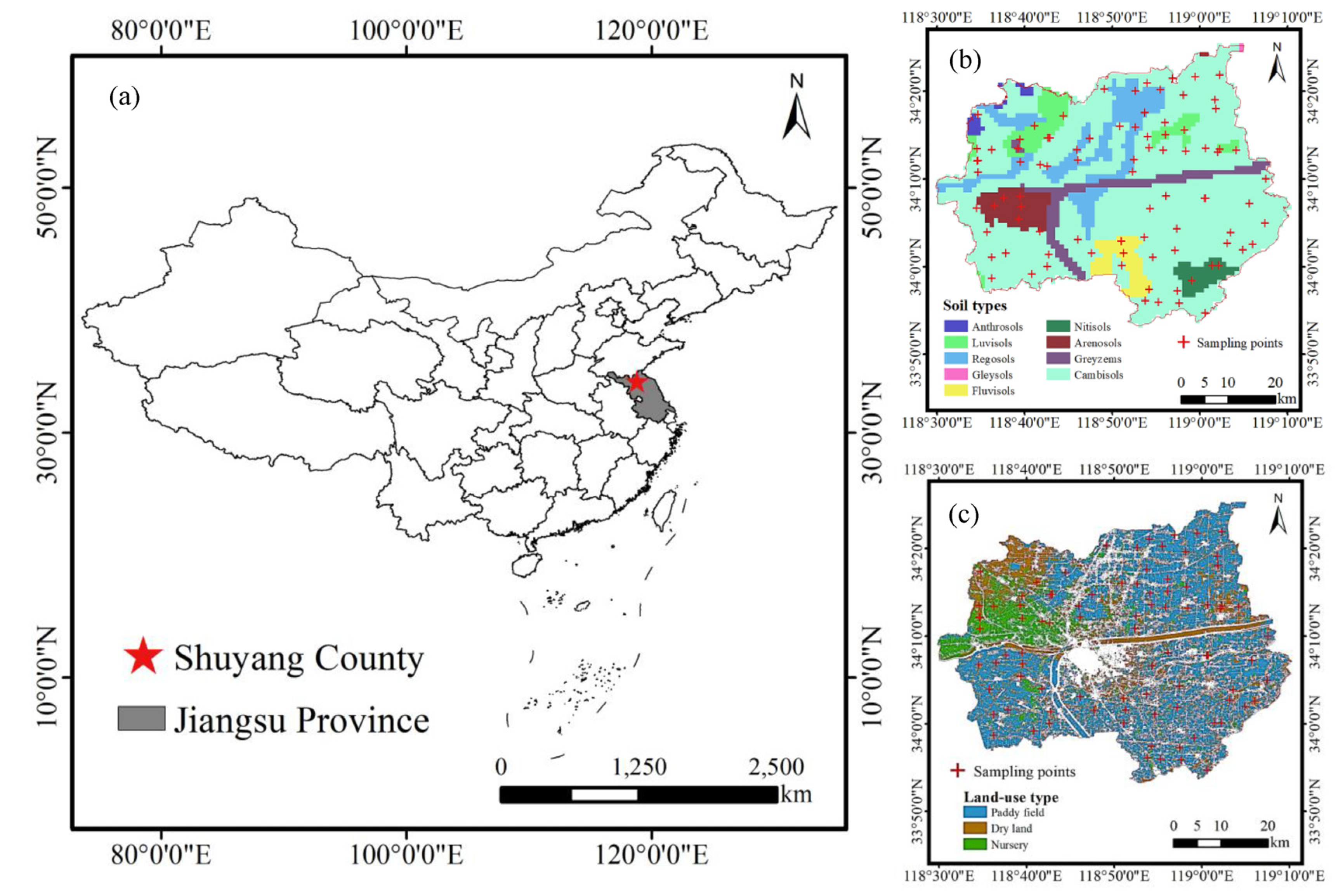
2.1. Study Area

The study area, Shuyang County (33°53’–34°25’ N, 118°30’–119°10’ E), is located in the northern part of Jiangsu Province (as shown in Figure 1a). The county spans 60 km from east to west and 55 km from north to south, covering an area of 2298 km². The terrain is higher in the west and lower in the east, and the ground elevation is mostly between 4.5 and 7 m. The river network is dense. The whole area lies in a temperate monsoon climate zone with abundant sunshine and average annual precipitation of 937.60 mm [30,31,32]. The soil texture of the topsoil (0–15 cm) in Shuyang County is mainly silt, and the contents of clay and sand are relatively small. The soil types include cambisols, regosols, luvisols, greyzems, anthrosols, gleysols, fluvisols, nitisols and arenosols (Figure 1b) [33,34], and the crops are mainly rice, wheat, maize and soybean [35]. The land-use types of cultivated land in the study area mainly include paddy fields, dry land and nurseries (Figure 1c).

2.2. Hyperspectral Satellite Data Acquisition and Preprocessing

The hyperspectral satellite image used in this study (Figure 2a) was acquired by the AHSI of ZY1-02D on October 22, 2020. The detailed parameters of AHSI/ZY1-02D data are shown in

Table 1. The parameters of Advanced Hyperspectral Imager (AHSI) data of ZY1-02D satellite.

Spectral range	400–2500 nm
Number of bands	166
Spatial resolution	30 m
Spectral resolution	VNIR 10 nm
	SWIR 20 nm
Swath width	60 km
Orbital period	55 days

. The spectrum of AHSI ranges from 0.4 to 2.5 μm with 166 bands. The spectral resolution of the 76 bands in the visible and near-infrared (VNIR) region is 10 nm, whereas the spectral resolution of the 90 bands in the shortwave infrared (SWIR) region is 20nm. The swath width of AHSI is 60 km, and the spatial resolution is 30 m.

Radiometric calibration and atmospheric correction (using the MODTRAN radiative transfer model) were carried out on the L1A data to obtain surface reflectance. Due to the low spectral response or atmospheric absorption of the sensor, only 130 bands in the spectral ranges of 464–997 nm, 1022–1106 nm, 1173–1324 nm, 1459–1778 nm and 1963–2468 nm were used in the study. A Savitzky–Golay filter [36] (the number of points on the left and right sides of the filter core center point was 3, the order of the derivative was set to 0, and the degree of smoothing polynomial was 1) was used to remove noise and smooth the spectrum, followed by orthorectification. Then the images were seamlessly mosaicked and cropped to obtain the preprocessed reflectance image of the whole Shuyang County. After this, we generated a binary map of cultivated and non-cultivated land of the study area according to the ground survey data. Finally, we masked the reflectance image with the binary map, and only the cultivated land area was kept for subsequent experiments. All the images were co-registered and rectified to the world geodetic system (WGS) 1984 datum.

Shuyang County was in the dry season when the satellite images acquired. The bare soil area in the image is mainly the soil that has just been plowed after the maize harvest, and the vegetation-covered area includes rice crops and tree seedlings. At the imaging time, the vegetation was in the growing season. The spectra of vegetation pixels have the typical vegetation spectral absorption characteristics (such as the red edge and green peak). Firstly, the training samples of bare soil and vegetation-covered areas were selected based on the comparison between pixel spectra and the standard spectral library (such as the USGS spectral library), in addition to the visual interpretation of the high-resolution satellite images (Gaofen-1 and Gaofen-2). Subsequently, the red edge normalized difference vegetation index (RENDVI) [37,38] was calculated based on the reflectance image of the whole study area. The classification accuracy of 96.59% was calculated using 88 randomly selected test samples. It can be seen from Figure 2c that the bare soil area was mainly distributed in the south, whereas the vegetation-covered area was distributed in the north.

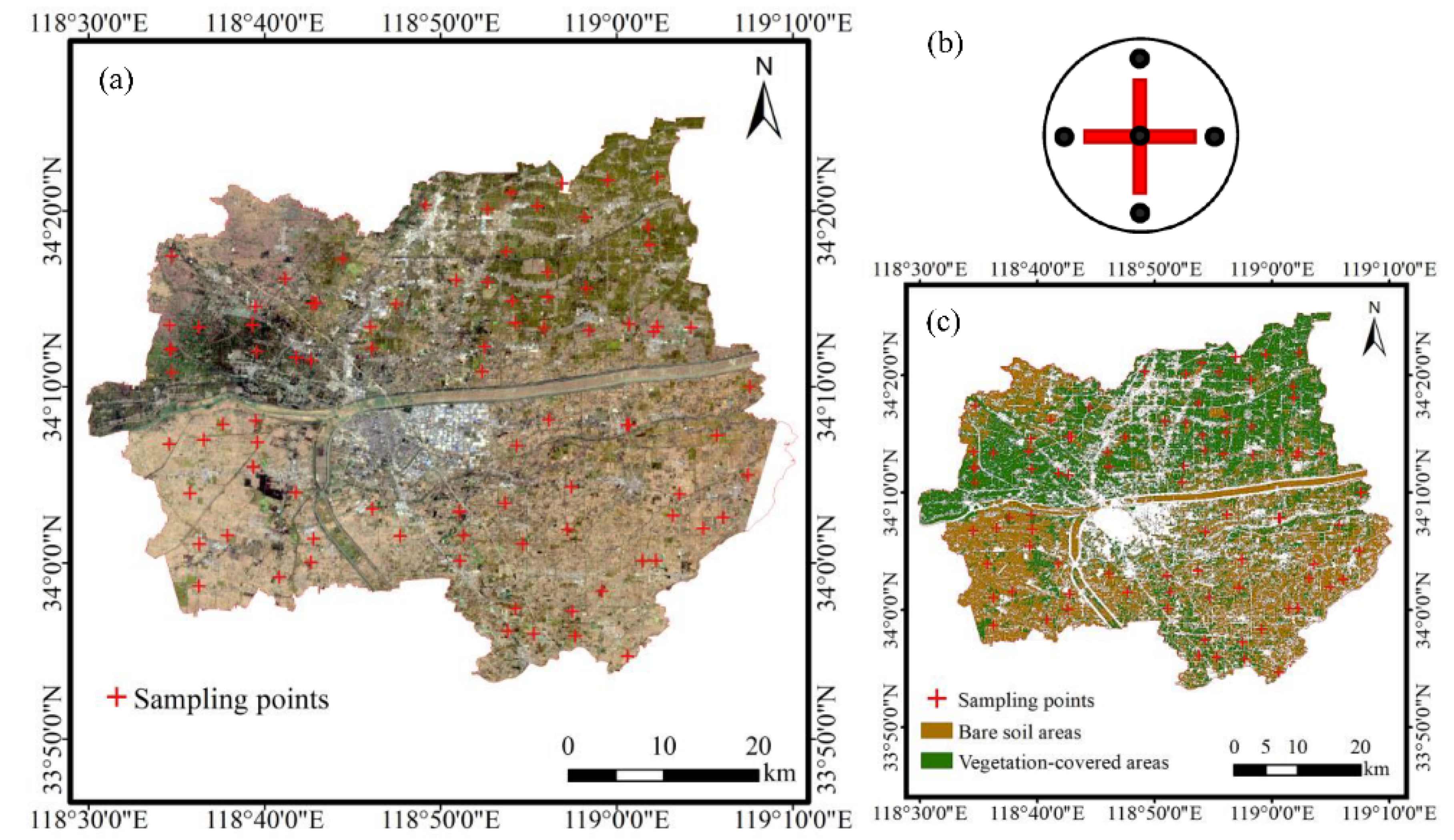
2.3. Ground Sampling and Soil Measurements

In July 2020, 92 surface soil samples (0–15 cm) were collected through a random sampling scheme (the minimum distance between the sampling points was set as 2 km). At each sampling point (red crosses in Figure 1 and Figure 2), five soil samples were collected in a circular area with a diameter of 10 m using the five-point method (Figure 2b), and the five samples were then mixed into one composite sample [39]. A one-kilogram composite sample of each spot was taken, dried indoors, and passed through a 2 mm sieve to remove gravel and plant residues. Then, the SOC content of the samples was determined in the fine fraction by the potassium dichromate-volumetric method [40]. Finally, the SOMC was obtained by multiplying a transformation coefficient of 1.724 (Van Bemmelen factor) to the SOC content [41]. According to Figure 2c, 92 sampling points were divided into two categories, with 38 sampling points in the bare soil area and 54 sampling points in the vegetation-covered area.

2.4. Methods

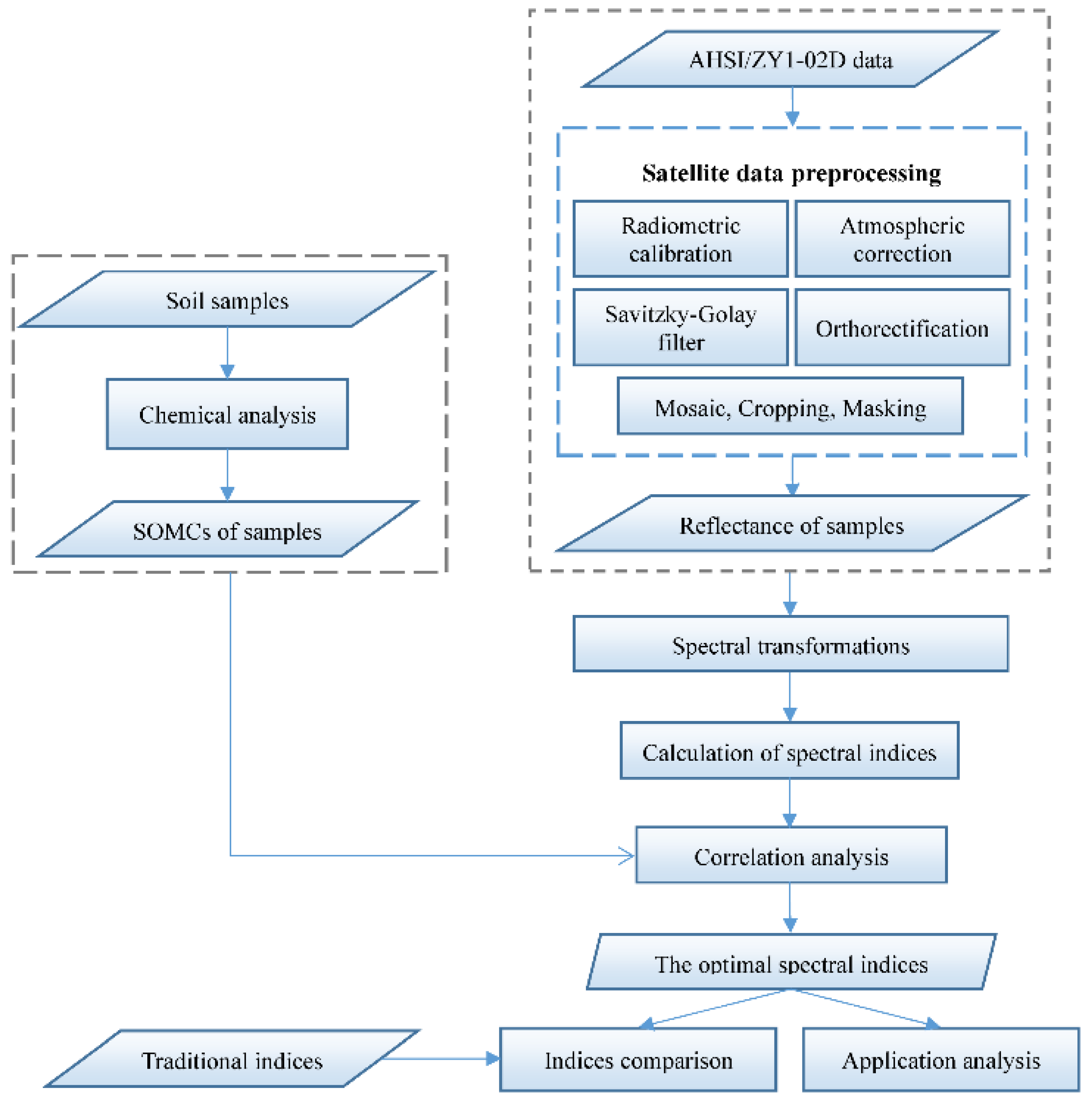
2.4.1. Research Process

The flow chart of this research is shown in Figure 3. The whole process can be divided into three main steps: (1) obtaining SOMC and reflectance spectra of soil samples, (2) constructing the optimal SIs, and (3) evaluating the application effect of the optimal SIs.

2.4.2. Construction of the Optimal SIs

Considering that the reflectance of some wavelengths is not sensitive to SOMC, spectral transformations are implemented on the original reflectance (OR). The spectral transformations can enhance the detailed information of the spectrum and help to extract the spectral features of SOM [39,42]. Before the transformation, low-quality bands are removed to avoid more noise and uncertainty. It should be noted that image spectroscopy is a powerful tool for estimating the spatial distribution of SOMC. In addition to obtain spectral information, it can also observe continuous spatial distribution information [43,44]. Therefore, the impact of each operation on the image quality needs to be considered in the construction of SIs. It is necessary to ensure that surface reflectance images and the optimal SIs do not lose the ability to intuitively express surface information. In this study, the images with better quality were those without noticeable mosaic lines, stripe noise and other phenomena that blur the actual feature information in terms of visual effects.

In

Table 2. The spectral transformations involved in this research ¹.

Type	Expression
Original reflectance (OR)	R
Reciprocal reflectance (RR)	1/R
Square root reflectance (SRR)	$\sqrt{R}$
First-order differential reflectance (FDR)	${R^{\prime }}_{{\lambda }_i}=\frac{1}{2}\times \left(\frac{R_{{\lambda }_{i+1}}-R_{{\lambda }_i}}{{\lambda }_{i+1}-{\lambda }_i}+\frac{R_{{\lambda }_i}-R_{{\lambda }_{i-1}}}{{\lambda }_i-{\lambda }_{i-1}}\right)$
First-order differential of reciprocal reflectance (RFDR)	$\left(1/R_{{\lambda }_i}\right)’=\frac{1}{2}\times \left(\frac{\left(1/R_{{\lambda }_{i+1}}\right)-\left(1/R_{{\lambda }_i}\right)}{{\lambda }_{i+1}-{\lambda }_i}+\frac{\left(1/R_{{\lambda }_i}\right)-\left(1/R_{{\lambda }_{i-1}}\right)}{{\lambda }_i-{\lambda }_{i-1}}\right)$
First-order differential of square root reflectance (SRFDR)	$\left(\sqrt{R_{{\lambda }_i}}\right)’=\frac{1}{2}\times \left(\frac{\sqrt{R_{{\lambda }_{i+1}}}-\sqrt{R_{{\lambda }_i}}}{{\lambda }_{i+1}-{\lambda }_i}+\frac{\sqrt{R_{{\lambda }_i}}-\sqrt{R_{{\lambda }_i-1}}}{{\lambda }_i-{\lambda }_{i-1}}\right)$
Second-order differential reflectance (SDR)	${R^{″}}_{{\lambda }_i}=\frac{1}{2}\times \left(\frac{R{’}_{{\lambda }_{i+1}}-R{’}_{{\lambda }_i}}{{\lambda }_{i+1}-{\lambda }_i}+\frac{R{’}_{{\lambda }_i}-R{’}_{{\lambda }_{i-1}}}{{\lambda }_i-{\lambda }_{i-1}}\right)$

¹ i−1 and i+1 denote the former and latter band of band i, λ is the wavelength.

, the formulas of different spectral transformations are listed. We calculated the correlations between SOMC and the reflectance spectra of different spectral transformations (including OR). Then, we analyzed the distribution of the correlation between different spectra and SOMC, and checked the quality of the transformed reflectance image. The spectra with higher correlations and better image quality were selected to calculate SIs. Next, further statistical analyses were conducted on all index formulas, and finally, we selected four index formulas, as shown in

Table 3. The construction formulas of spectral indices (SIs) ¹.

SIs	Expression
Difference index (DI)	$p-q$
Ratio index (RI)	$\frac{p}{q}$
Normalized difference index (NDI)	$\frac{p-q}{p+q}$
Square root index of difference (DSI)	$\sqrt{p-q}$

¹ p and q are the transformed spectra values corresponding to any two bands and p ≠ q.

. The correlation between each type of spectral index (SI) and SOMC was analyzed, and the indices with higher correlation and better image quality were chosen as the optimal SIs.

Pearson’s correlation coefficient ($\rho$) was adopted to determine the correlation between two variables in the correlation analysis. Its formula is as follows:

$$●\hspace{1em}{\rho }_{X,Y}=\frac{cov\left(X,Y\right)}{{\sigma }_X{\sigma }_Y}=\frac{E\left(\left(X-{\mu }_X\right)\left(Y-{\mu }_Y\right)\right)}{{\sigma }_X{\sigma }_Y},$$

(1)

where ${\sigma }_X$, ${\sigma }_Y$ are the standard deviations of the X and Y arrays, respectively; ${\mu }_X$, ${\mu }_Y$ are the mean values of X, Y, respectively.

2.4.3. Application Assessment of the Optimal SIs

In order to evaluate the ability of the optimal SIs to characterize SOMC, we analyzed the application performance from two aspects. One compares the optimal SIs with the traditional SOM indices. In bare soil and vegetation-covered areas, we selected an optimal SI with the highest correlation. We calculated the correlation between other traditional indices and SOMC for comparison, and the bases for the selection of traditional indices are listed in Table 4. The linear regression (LR) model describing the relationship between each index and SOMC was established individually, and the corresponding determination coefficient (R²) was calculated to evaluate the performance of each index. In addition, the LR models of the optimal SIs here were also applied to obtain the inversion map of SOMC for recognition of SOMC levels.

The other utilizes the optimal SIs to construct the prediction models of SOMC to evaluate their application performance. All the optimal SIs were selected to construct the corresponding model in the bare soil and vegetation-covered areas. Considering the data redundancy caused by the high correlation between indices, principal component analysis (PCA) was adopted for dimensionality reduction. PCA linearly transforms predictors to remove redundant dimensions, and generates a new set of variables called principal components [45,46].

In terms of the inversion model, SVM and tree ensembles (TE) show good performance in soil attributes’ estimation by satellite remote sensing. George et al. [47] used different hyperspectral indices generated by EO-1 Hyperion data and the SVM method to draw various soil salinity severity levels in the Mathura region of the Indo-Gangetic plain of India, and the overall classification accuracy was 78.13%. Based on GF-5 data, Meng et al. [48] used the TE model to predict SOMC in Mingshui County, Heilongjiang Province, China, and the root mean square error of the model was 3.36 g/kg. In this study, six SVM models (linear SVM, quadratic SVM, cubic SVM, fine Gaussian SVM, medium Gaussian SVM, coarse Gaussian SVM) and two TE models (boosted trees, bagged trees) were compared for SOMC estimation in bare soil and vegetation-covered areas. In order to avoid overfitting, the K-fold cross-validation method was used to verify the modeling accuracy. For the bare soil and vegetation-covered areas, the model with the highest accuracy of each was applied to the image of the corresponding area. The inversion results of bare soil and vegetation-covered areas were merged to obtain the SOMC distribution of the whole area.

Furthermore, we adopted the R², the root mean square error (RMSE), and the residual prediction deviation (RPD) to evaluate the SOMC characterization ability of the inversion model constructed by the optimal SIs. In general, a well-established model usually has a high R² and RPD, and a low RMSE [23,39]. According to the research of Yuan et al. [49], the RPD values are divided into five levels to interpret the model performance, RPD < 1.4 (unacceptable), 1.4 ≤ RPD < 1.8 (fair), 1.8 ≤ RPD < 2.0 (good), 2.0 ≤ RPD < 2.5 (very good), and RPD ≥ 2.5 (excellent). Their calculation formulas are as follows:

$$●\hspace{1em}{R}^2=1-\frac{{{\displaystyle \sum }}_{i=1}^n{\left({\widehat{y}}_i-y_i\right)}^2}{{{\displaystyle \sum }}_{i=1}^n{\left(y_i-\overline{y}\right)}^2},$$

(2)

$$●\hspace{1em}RMSE=\sqrt{\frac{{{\displaystyle \sum }}_{i=1}^n{\left(y_i-{\widehat{y}}_i\right)}^2}{n}},$$

(3)

$$●\hspace{1em}RPD=\frac{\sqrt{{{\displaystyle \sum }}_{i=1}^n{\left(y_i-\overline{y}\right)}^2/n}}{RMSE},$$

(4)

where $y_i$ is the actual value, the $\overline{y}$ is the mean value of $y_i$, ${\widehat{y}}_i$ is the fitted value, and $n$ is the number of samples.

Table 4. The formulas of the traditional SIs.

Index Type	Abbreviation	Formula	Properties	References
Soil SI	SOC1	$\frac{1}{{{\displaystyle \sum }}_{400nm}^{700nm}R}$	SOMC	[22]
	SOC2	$\frac{1}{\left(R_{600nm}-R_{400nm}\right)/\left(600-400\right)}$	SOMC	[22]
	SOC3	$\frac{1}{\left(R_{2200nm}-R_{2138nm}\right)/\left(2200-2138\right)}$	SOMC	[22]
	NSMI	$\frac{R_{1800nm}-R_{2119nm}}{R_{1800nm}+R_{2119nm}}$	Soil moisture	[50,51]
Vegetation SI	CAI	$\frac{R_{2000nm}+R_{2200nm}}{2}-R_{2100nm}$	Cellulose Absorption	[52,53,54]
	NDLI	$\frac{\log \left(1/R_{1754nm}\right)-\log \left(1/R_{1680nm}\right)}{\log \left(1/R_{1754nm}\right)+\log \left(1/R_{1680nm}\right)}$	Lignin concentration	[53,55,56,57]
	MSI	$\frac{R_{1610nm}}{R_{868nm}}$	Leaf water content	[58,59]
	SATVI	$\frac{R_{1610nm}-R_{665nm}}{R_{1610nm}+R_{665nm}}\times 2-\frac{R_{2190nm}}{2}$	Total vegetation cover	[58,60]

Table 4. The formulas of the traditional SIs.

Index Type	Abbreviation	Formula	Properties	References
Soil SI	SOC1	$\frac{1}{{{\displaystyle \sum }}_{400nm}^{700nm}R}$	SOMC	[22]
	SOC2	$\frac{1}{\left(R_{600nm}-R_{400nm}\right)/\left(600-400\right)}$	SOMC	[22]
	SOC3	$\frac{1}{\left(R_{2200nm}-R_{2138nm}\right)/\left(2200-2138\right)}$	SOMC	[22]
	NSMI	$\frac{R_{1800nm}-R_{2119nm}}{R_{1800nm}+R_{2119nm}}$	Soil moisture	[50,51]
Vegetation SI	CAI	$\frac{R_{2000nm}+R_{2200nm}}{2}-R_{2100nm}$	Cellulose Absorption	[52,53,54]
	NDLI	$\frac{\log \left(1/R_{1754nm}\right)-\log \left(1/R_{1680nm}\right)}{\log \left(1/R_{1754nm}\right)+\log \left(1/R_{1680nm}\right)}$	Lignin concentration	[53,55,56,57]
	MSI	$\frac{R_{1610nm}}{R_{868nm}}$	Leaf water content	[58,59]
	SATVI	$\frac{R_{1610nm}-R_{665nm}}{R_{1610nm}+R_{665nm}}\times 2-\frac{R_{2190nm}}{2}$	Total vegetation cover	[58,60]

3. Results

3.1. Descriptive Statistics of Samples

Table 5. The statistics of soil organic matter content (SOMC) in Shuyang County.

	All Samples	Samples in Bare Soil Areas	Samples in Vegetation-Covered Areas
Number of samples	92	38	54
Range (g/kg)	10.27–47.80	10.27–34.40	10.96–47.80
Mean (g/kg)	25.17	23.45	26.36
Standard deviation(g/kg)	7.88	6.65	8.49
Coefficient of variation (%)	31.32	28.36	32.22

illustrates the statistics of SOMC of soil samples in Shuyang County. The SOMC exhibits a range from 10.27 to 47.80 g/kg. The mean value and the standard deviation are 25.17 and 7.88 g/kg, respectively. The moderate coefficient of variation is 31.32%. These samples are further categorized into bare soil and vegetation-covered areas. The minimum SOMC of samples from both regions are similar, and both are moderate variations. However, the maximum SOMC in the vegetation-covered area can reach 47.80g/kg, which is much higher than that in the bare soil area. Moreover, the mean of SOMC in the vegetation-covered area is about 3.00 g/kg greater than that in the bare soil area.

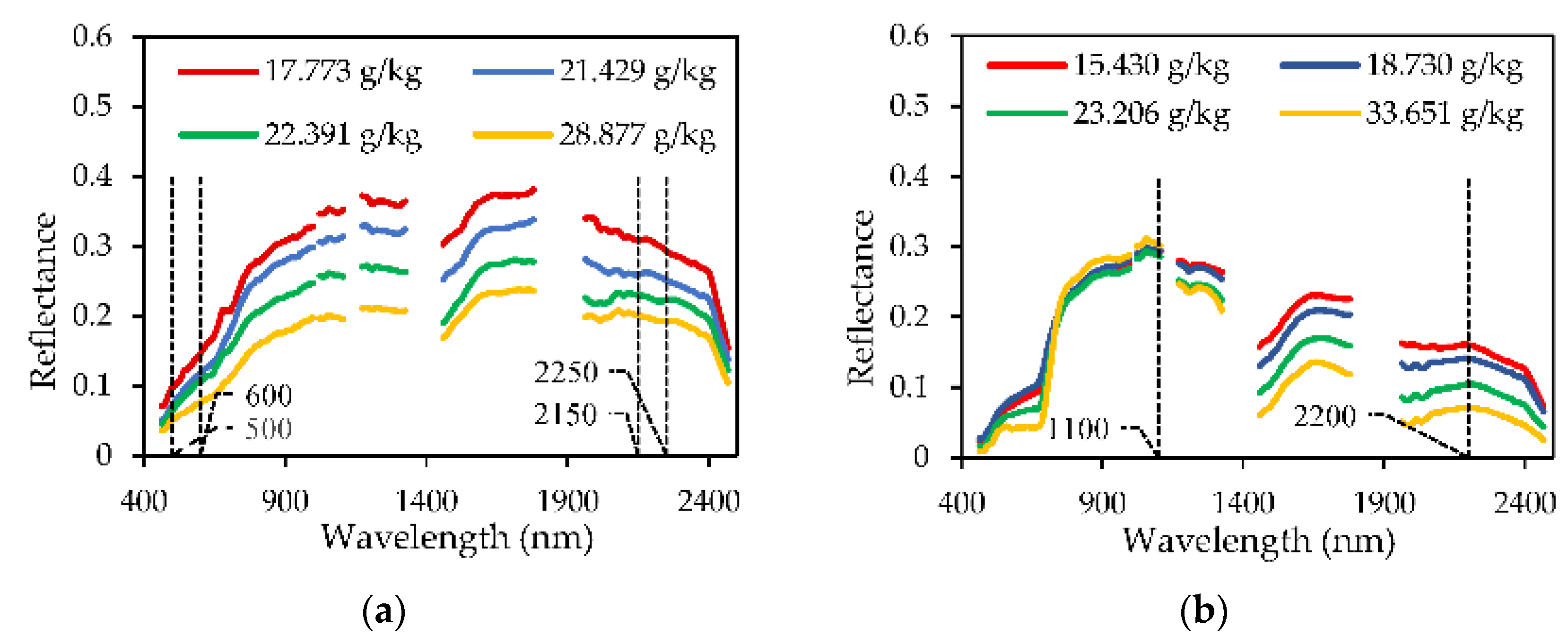
3.2. Spectral Characteristics of the Pixel Reflectance of the Sample Sites

Based on the processed images, the reflectance spectra of the pixels at 92 sampling points were extracted. In the bare soil area, it can be seen from Figure 4a that the reflectance spectrum decreases with the increase in SOMC in the entire 400–2500 nm range. In the range of 500–600 nm, the slope of the curve decreases with the increase in SOMC. There is a spectral absorption in the range of 2150–2250 nm. These are consistent with the results of previous studies. Bartholomeus et al. [22] found that in the 400–700 nm range, there was a flatter spectral profile at higher SOMC, and Jin et al. [23] found that there was a spectral absorption at 2200 nm. On the whole, the extracted reflectance spectral curves can clearly depict the soil spectral variation patterns at different SOMCs.

In the vegetation-covered area, as shown in Figure 4b, the reflectance spectrum decreases with the increase in SOMC in the range of 1100–2500 nm. In previous studies, Bartholomeus et al. [53] also found that in the range of 2000–2200 nm, with the increase in SOMC, cellulose also increased, resulting in low reflectance in this spectral region. In general, the extracted reflectance spectral curves can well demonstrate the vegetation spectral variation patterns at different SOMCs.

3.3. Correlation between Transformed Spectra and SOMC

Because complex spectral transformations such as the second-order differential may introduce more noise into the image [39], these bands need to be removed (as shown in

Table 6. The wavelength range and the number of low-quality bands of each transformed spectrum.

Spectral Transformation Type	Wavelengths of Bands of Low Quality (nm)	The Number of Bands Removed
OR/RR/SRR	395–456; 1006–1014; 1122–1156; 1341–1442; 1795–1947; 2484–2501	36
FDR	395–559; 585–637; 679; 748–1089; 1122–1156; 1207–1308; 1341–1442; 1475–1526; 1660–1762; 1795–1947; 1981; 2014–2082; 2233–2384; 2484–2501	125
RFDR	395–473; 550–662; 748–757; 774; 791–808; 885; 920; 996–1022; 1122–1156; 1341–1442; 1475–1510; 1762–1947; 1981; 2014–2031; 2132–2250; 2334–2401; 2434–2501	86
SRFDR	395–508; 524–559; 576–637; 748–1089; 1122–1156; 1190–1308; 1341–1442; 1475–1526; 1660–1712; 1762; 1795–1947; 1981; 2014–2082; 2216–2401; 2450–2501	127
SDR	395–456; 473–671; 696–1073; 1106; 1122–1156; 1207–1291; 1341–1442; 1492–1745; 1795–1947; 1998; 2031–2216; 2249–2367; 2434–2501	147

). In OR, RR and SRR, most of the bands removed are due to the low spectral response or atmospheric absorption of the sensor, and the total number of low-quality bands is 36. However, after differential transformation, the number of low-quality bands is significantly increased. Among these, FDR is the least increased. The number of low-quality bands in SDR reaches 147, increasing the most, and its image quality is relatively poor. The correlations between SOMC and the transformed spectra are shown in

Table 7. Correlation with SOMC after different spectral transformations.

TRs	Nb.1	Bare Soil Region			Vegetation-Covered Area
		Nsb 2	$\mathbf{Maximum} \left|\mathit{\rho }\right|$	WLsb 3 (nm)	Nsb 2	$\mathbf{Maximum} \left|\mathit{\rho }\right|$	WLsb 3 (nm)
OR	130	0			52	0.558 ***	533–610, 696–1106 (722)
RR	130	0			62	0.573 ***	524–1106 (722)
SRR	130	0			56	0.563 ***	524–636, 696–1106 (722)
FDR	41	3	0.350 *	662, 1459, 1779	6	0.502 ***	687, 696, 1106, 1173, 1190, 132445
RFDR	80	2	0.370 *	2048, 2317	3	0.381 **	687, 1694, 1745
SRFDR	39	5	0.462 **	654, 662, 671, 1459, 1779	5	0.477 ***	516, 1106, 1173, 1324, 1745
SDR	19	6	0.493 **	1173, 1190, 1308, 1425, 1762, 1779	4	0.462 ***	1173, 1190, 1762, 1779

¹ Nb stands for the number of available bands. ² Nsb stands for the number of sensitive bands. ³ WLsb stands for the wavelength of the sensitive band. Value: Wavelength of the maximum correlation coefficient. ^* Correlation is significant at 0.05 level. ^** Correlation is significant at 0.01 level. ^*** Correlation is significant at 0.001 level.

.

In the bare soil area, OR, RR and SRR do not have the bare soil spectra that have significant correlations with SOMC, whereas differential transformations can obtain some sensitive bands (|$\rho$| > 0.320, p < 0.05). The first-order differential transformation on the basis of OR, RR and SRR can effectively improve the correlation with SOMC. For spectra after differential transformations of different orders, the results show that the higher the order, the higher the correlation with SOMC, indicating the differential transformation is an effective means to improve the correlation with SOMC for soil spectra. As shown by the overall results of the different transformations, it can be found that these sensitive wavelengths are mainly concentrated around 660, 1459 and 1779 nm, which is consistent with the studies of Jin et al. [23], Wang et al. [39] and Guo et al. [61].

In the vegetation-covered area, OR, RR and SRR can improve the correlation with SOMC and increase the number of sensitive bands (|$\rho$| > 0.268, p < 0.05). However, the first-order differential transformation based on RR and SRR will decrease the correlation with SOMC and reduce the number of sensitive bands. For spectra after differential transformations of different orders, the results show that the higher the order, the smaller the correlation with SOMC. It can be seen from the overall results of different transformations that these sensitive wavelengths are mainly concentrated around 680 nm and 1745–1779 nm, which are consistent with the sensitive wavelengths obtained in the studies of Bartholomeus et al. [53], Zhang et al. [26] and Fourty et al. [55]. Considering the correlation with SOMC and the image quality, OR, RR, FDR and RFDR were chosen to calculate the SIs.

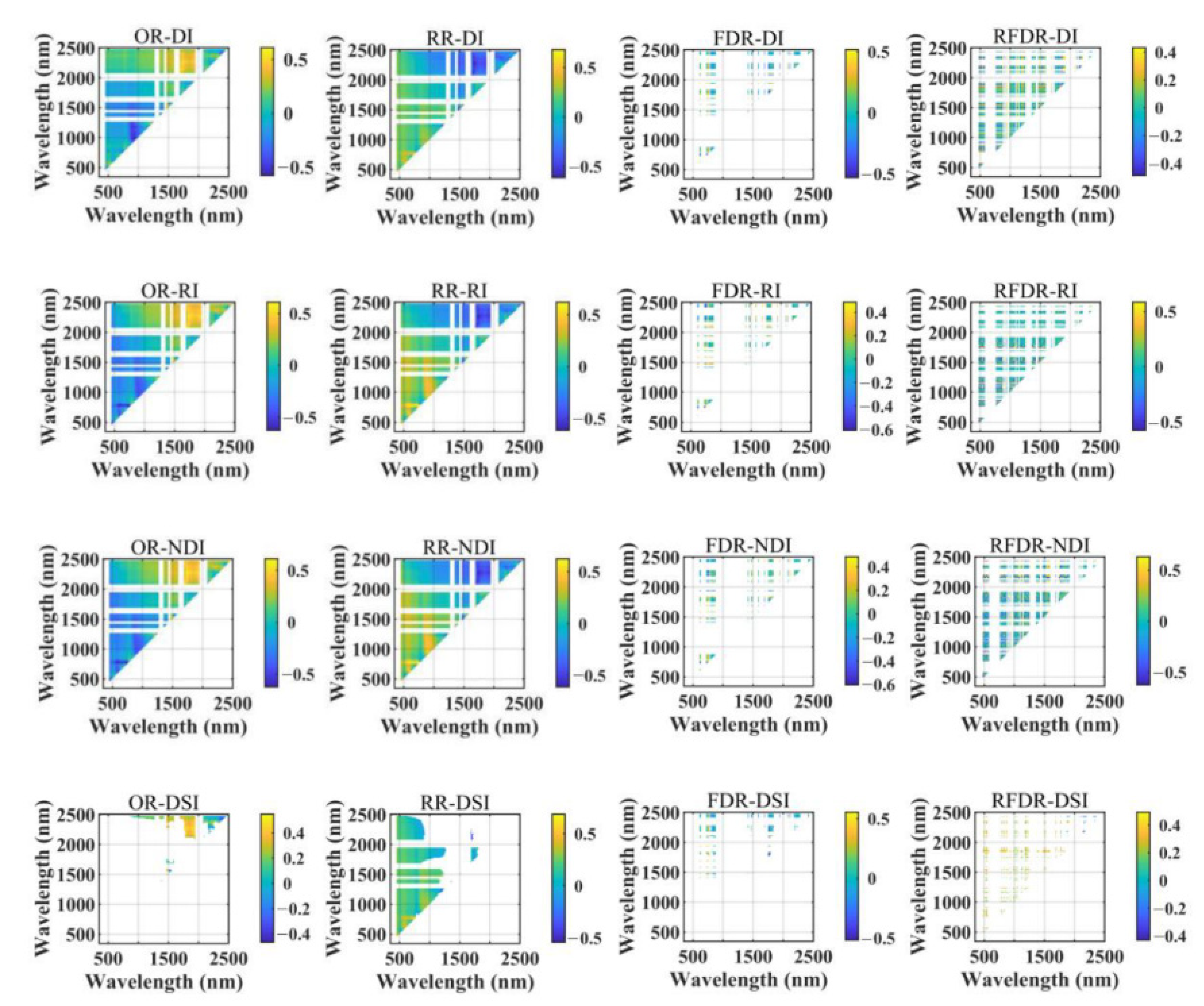
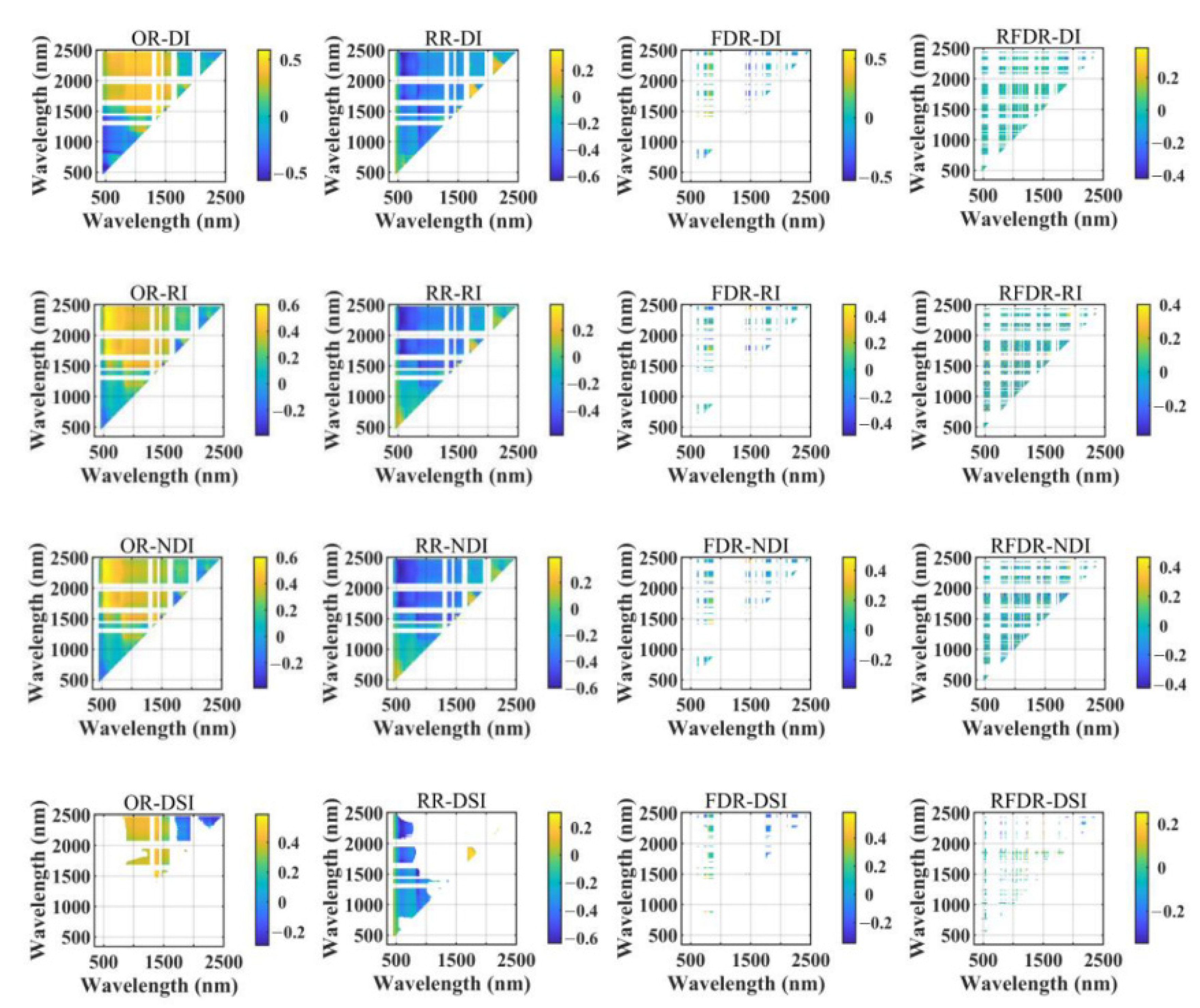
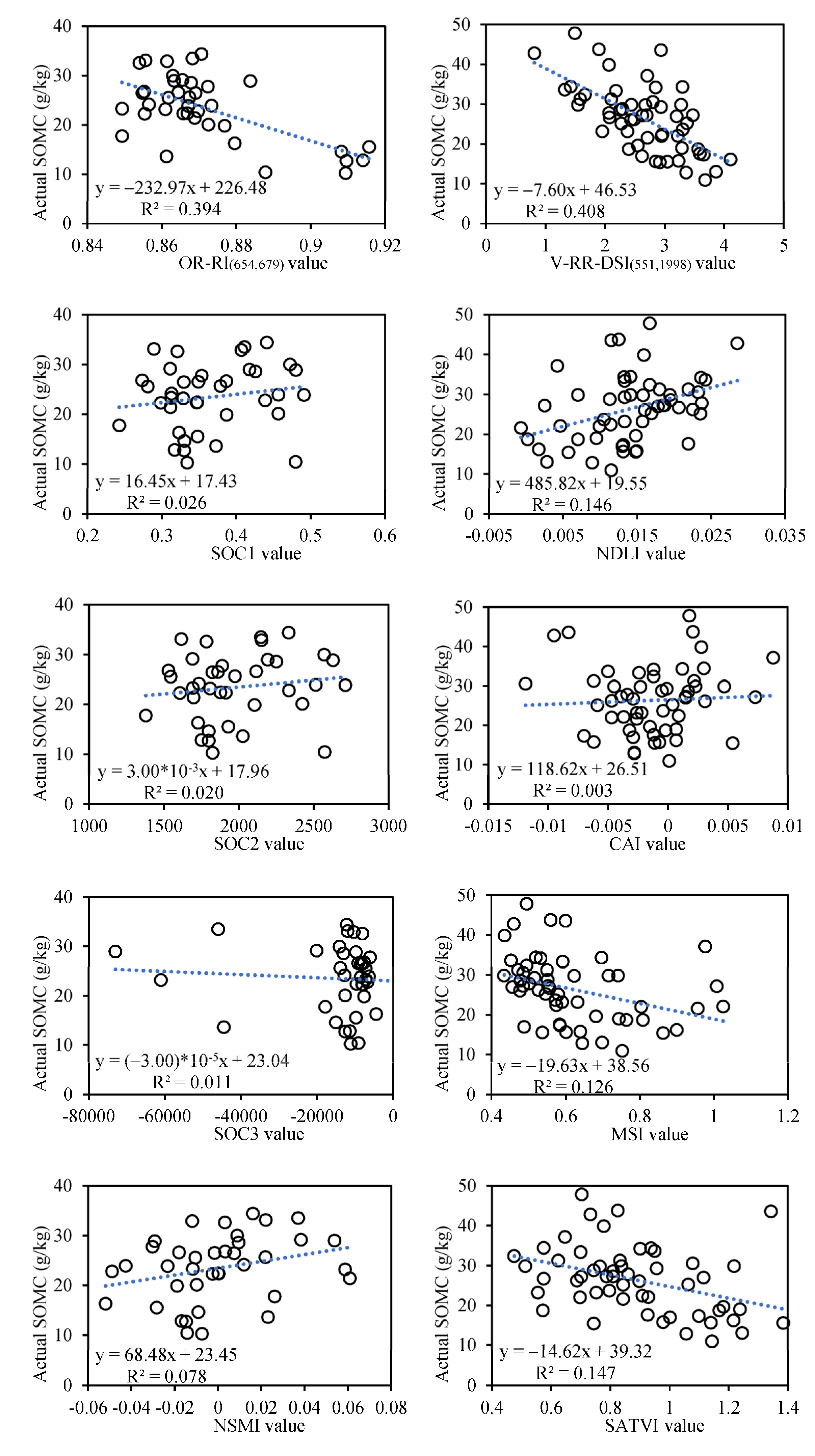
3.4. Correlation between SIs and SOMC

Sixteen types of SIs were calculated by four transformed spectra (OR, RR, FDR and RFDR) and four index formulas (DI, RI, NDI and DSI). All available bands of the transformed spectra were substituted into the calculation. Then, their correlations with the SOMC of soil samples in bare soil and vegetation-covered areas were analyzed. The correlation coefficient matrix diagrams are shown in Figure 5 and Figure 6. In addition, the maximum correlation coefficient (|$\rho$|_max) between each type of SI and SOMC in bare soil and vegetation-covered areas is listed in

Table 8. The maximum correlation index of different types of SIs in the bare soil area.

Type		$\mathbf{Number} \mathbf{of} \mathbf{SIs} \mathbf{with} \left|\mathit{\rho }\right|>0.6$	$|\mathit{\rho }{|}_{\mathbf{max}}$	$\mathbf{Index} \mathbf{Formula} \mathbf{Corresponding} \mathbf{to} |\mathit{\rho }{|}_{\mathbf{max}}$
OR	DI	1	0.612 ***	$R_{1459nm}-R_{2014nm}$
	RI	6	0.627 ***	$R_{654nm}/R_{679nm}$
	NDI	5	0.626 ***	$\left(R_{654nm}-R_{679nm}\right)/\left(R_{654nm}+R_{679nm}\right)$
	DSI	0	0.548 ***	$\sqrt{R_{1543nm}-R_{2216nm}}$
RR	DI	3	0.614 ***	$1/R_{1493nm}-1/R_{2014nm}$
	RI	6	0.623 ***	$\left(1/R_{679nm}\right)/\left(1/R_{654nm}\right)$
	NDI	5	0.626 ***	$\frac{1/R_{654nm}-1/R_{679nm}}{1/R_{654nm}+1/R_{679nm}}$
	DSI	0	0.426 **	$\sqrt{1/R_{559nm}-1/R_{671nm}}$
FDR	DI	0	0.518 ***	$R{’}_{662nm}-R{’}_{1779nm}$
	RI	0	0.488 **	$R{’}_{1190nm}/R{’}_{2216nm}$
	NDI	1	0.603 ***	$\left(R{’}_{662nm}-R{’}_{2216nm}\right)/\left(R{’}_{662nm}+R{’}_{2216nm}\right)$
	DSI	0	0.555 ***	$\sqrt{R{’}_{662nm}-R{’}_{1779nm}}$
RFDR	DI	0	0.488 **	${\left(1/R_{2048nm}\right)}^{’}-\left(1/R_{2081nm}\right)’$
	RI	0	0.587 ***	${\left(1/R_{765nm}\right)}^{’}/{\left(1/R_{1291nm}\right)}^{’}$
	NDI	2	0.625 ***	$\frac{{\left(1/R_{1106nm}\right)}^{’}-\left(1/R_{2048nm}\right)’}{{\left(1/R_{1106nm}\right)}^{’}+\left(1/R_{2048nm}\right)’}$
	DSI	0	0.494 **	$\sqrt{{\left(1/R_{1728nm}\right)}^{’}-\left(1/R_{2301nm}\right)’}$

^** Correlation is significant at 0.01 level. ^*** Correlation is significant at 0.001 level.

and

Table 9. The maximum correlation index of different types of SIs in the vegetation-covered area.

Type		$\mathbf{Number} \mathbf{of} \mathbf{SIs} \mathbf{with} \left|\mathit{\rho }\right|>0.6$	$|\mathit{\rho }{|}_{\mathbf{max}}$	$\mathbf{Index} \mathbf{Formula} \mathbf{Corresponding} \mathbf{to} |\mathit{\rho }{|}_{\mathbf{max}}$
OR	DI	0	0.576 ***	$R_{722nm}-R_{2468nm}$
	RI	19	0.604 ***	$R_{525nm}/R_{2267nm}$
	NDI	3	0.601 ***	$\left(R_{525nm}-R_{2250nm}\right)/\left(R_{525nm}+R_{2250nm}\right)$
	DSI	0	0.569 ***	$\sqrt{R_{722nm}-R_{2468nm}}$
RR	DI	84	0.634 ***	$1/R_{722nm}-1/R_{1291nm}$
	RI	0	0.587 ***	$\left(1/R_{525nm}\right)/\left(1/R_{1510nm}\right)$
	NDI	3	0.601 ***	$\frac{1/R_{525nm}-1/R_{2250nm}}{1/R_{525nm}+1/R_{2250nm}}$
	DSI	83	0.639 ***	$\sqrt{1/R_{551nm}-1/R_{1998nm}}$
FDR	DI	0	0.575 ***	$R{’}_{671nm}-R{’}_{1173nm}$
	RI	0	0.490 **	$R{’}_{1173nm}/R{’}_{1627nm}$
	NDI	0	0.489 ***	$\left(R{’}_{705nm}-R{’}_{1173nm}\right)/\left(R{’}_{705nm}+R{’}_{1173nm}\right)$
	DSI	0	0.581 ***	$\sqrt{R{’}_{671nm}-R{’}_{1173nm}}$
RFDR	DI	0	0.421 **	${\left(1/R_{1745nm}\right)}^{’}-\left(1/R_{2301nm}\right)’$
	RI	0	0.393 **	${\left(1/R_{868nm}\right)}^{’}/{\left(1/R_{1577nm}\right)}^{’}$
	NDI	0	0.468 ***	$\frac{{\left(1/R_{688nm}\right)}^{’}-\left(1/R_{1745nm}\right)’}{{\left(1/R_{688nm}\right)}^{’}+\left(1/R_{1745nm}\right)’}$
	DSI	0	0.348 **	$\sqrt{{\left(1/R_{1241nm}\right)}^{’}-\left(1/R_{1627nm}\right)’}$

^** Correlation is significant at 0.01 level. ^*** Correlation is significant at 0.001 level.

. Considering the performance of various types of SIs in the bare soil area and vegetation-covered area, |$\rho$| greater than 0.600 was utilized as the threshold to obtain the optimal SIs.

In the bare soil area, it can be seen from Figure 5 and Table 8 that for the same types of spectral transformation, NDI can maximize the correlation between SOMC and three types of transformed spectra (RR, FDR and RFDR). In addition, RI can also achieve a high correlation between SOMC and three types of transformed spectra (OR, RR and RFDR). In four index formulas, DSI has the lowest correlation with SOMC. Among the four types of SIs constructed based on RR, there are 14 SIs with a correlation greater than 0.6 with SOMC, followed by 12 SIs based on OR. For the same index formula, the indices calculated from OR and RR generally have higher correlations with SOMC than FDR and RFDR. In the bare soil area, OR-RI has the highest correlation with SOMC at the combination of 654 and 679 nm (OR-RI_(654,679)), with |$\rho$| as high as 0.627.

In the vegetation-covered area, it can be seen from Figure 6 and Table 9 that for the same types of spectral transformation, DSI can obtain the highest correlation between SOMC and two types of transformed spectra (RR and FDR). In addition, DI also attains a high correlation between SOMC and three types of transformed spectra (RR, FDR and RFDR). Among the four types of SIs constructed based on RR, the number of SIs with a correlation greater than 0.6 with SOMC is as many as 180, far more than other spectra. For the same index formula, the indices calculated from OR and RR have significantly higher correlations with SOMC than FDR and RFDR. In the vegetation-covered area, RR-DSI has the highest correlation with SOMC at the combination of 551 and 1998 nm (RR-DSI_(551,1998)), with |$\rho$| as high as 0.639.

Because the values of OR-NDI and RR-NDI are opposite to each other, and the wavelengths used are the same, it is sufficient to choose one of them. When modeling, the optimal SIs obtained by OR-NDI were adopted. Therefore, there are 24 optimal SIs for the bare soil area and 189 for the vegetation-covered area.

3.5. Application of the Optimal SIs

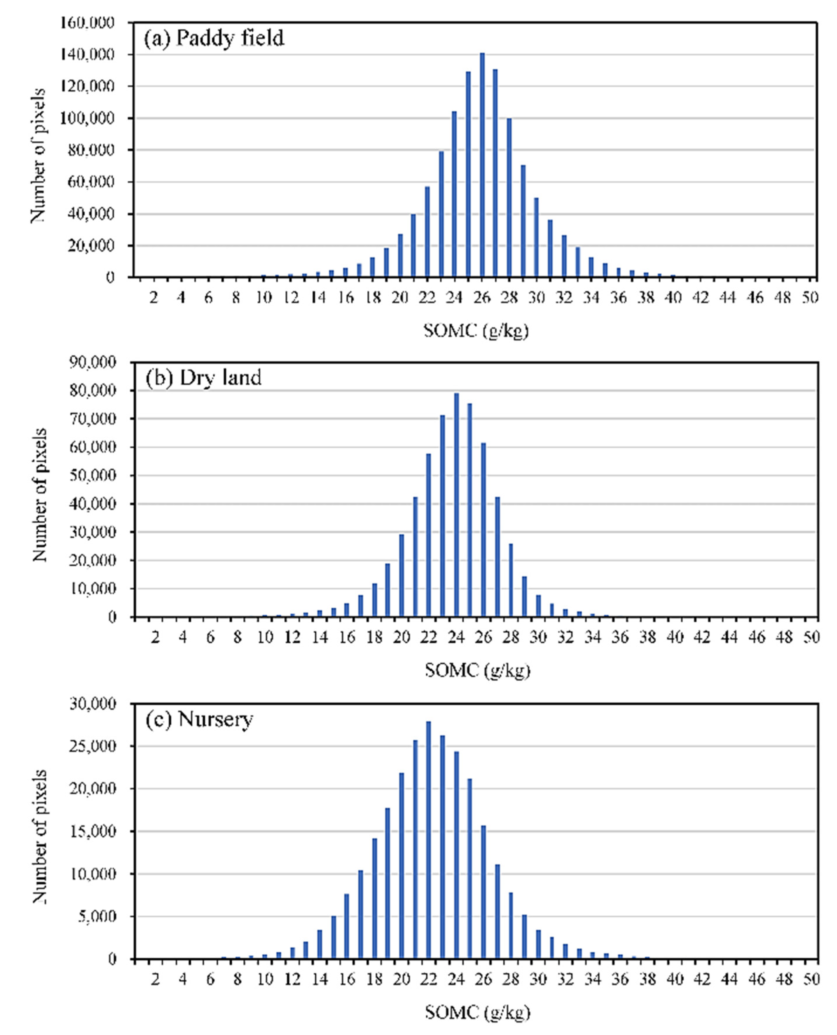
3.5.1. Characterization of SOMC in Soil Samples

According to Table 8 and Table 9, OR-RI_(654,679) and RR-DSI_(551,1998) have the highest correlation with SOMC in bare soil and vegetation-covered areas, respectively (the letter ’V’ is added to RR-DSI_(551,1998) as a prefix (V-RR-DSI_(551,1998)), which represents the optimal SI in the vegetation-covered area). These two indices were selected to construct LR models and compare them with other traditional indices (Table 4). The correlations of SOMC and different SIs are shown in Figure 7.

In the bare soil area, the R² of the model constructed by OR-RI_(654,679) is 0.398, much larger than the R² of the models constructed by other indices. In the vegetation-covered area, the R² of the model constructed by V-RR-DSI_(551,1998) is 0.408, whereas the other indices are all less than 0.2. In general, the OR-RI_(654,679) and V-RR-DSI_(551,1998) proposed in this study well characterize SOMC in bare soil and vegetation-covered areas, respectively.

3.5.2. Recognition of SOMC Levels in Soil Samples

According to the linear relations shown in Figure 7, SOMC in the bare soil area was calculated by OR-RI_(654,679), whereas SOMC in the vegetation-covered area was calculated by V-RR-DSI_(551,1998). After the SOMCs of bare soil and vegetation-covered areas were merged, SOMC of the whole cultivated land in Shuyang County was obtained. Based on the numerical distribution of SOMC, the calculated and measured SOMC was similarly divided into five levels by the equal interval method, as shown in Figure 8.

On the whole, the SOMC levels in the cultivated area of Shuyang County are consistent with the trend shown by SOMC of the soil samples (Figure 8a). They all display that the spatial distribution of the SOMC level in Shuyang County is high in the northeast, low in the northwest and intermediate in the south. The areas with the highest SOMC level are concentrated in vegetation-covered areas in the northeast, where most areas exceed 30 g/kg. The lowest SOMC level is found in bare soil areas in the northwest, mostly below 15 g/kg. The detailed image (Figure 8b) shows that the results calculated using OR-RI_(654,679) and V-RR-DSI_(551,1998) can well recognize soil samples with different SOMC levels.

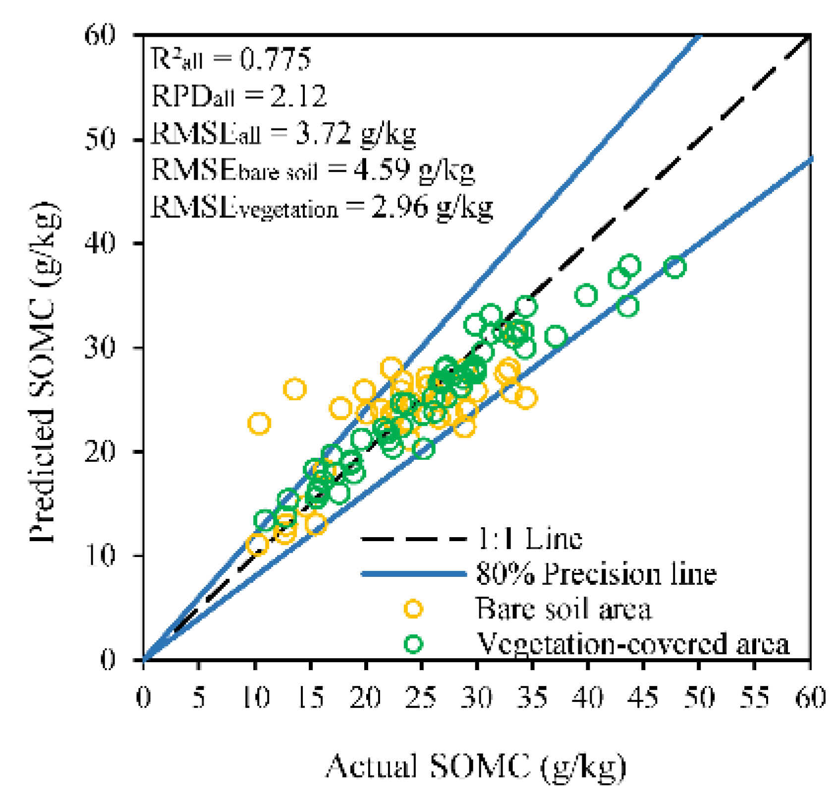
3.5.3. Estimation of SOMC in Soil Samples

As mentioned in Section 3.4, 24 soil SIs and 189 vegetation SIs were employed in the prediction model. The modeling data of bare soil and vegetation-covered areas are divided into 10 folds for cross-validation, respectively. PCA with a 99.99% explanatory variance rate was used for dimensionality reduction and a new set of variables was generated for modeling. Among the eight inversion models introduced in Section 2.4.3, the linear SVM and least-squares boosting tree algorithms obtained the highest prediction accuracy in bare soil and vegetation-covered areas, respectively.

The prediction accuracy of SOMC based on the soil-vegetation combined prediction is shown in Figure 9. Overall, the predicted results have a good linear relationship with the SOMC of samples. The R², RMSE and RPD of the soil-vegetation combined prediction results are 0.775, 3.72 g/kg and 2.12, respectively, suggesting the model is very good. Specifically, the RMSE of bare soil and vegetation-covered samples is 4.59 and 2.96 g/kg, respectively. Most scatters are very close to the 1:1 line, especially in the vegetation-covered area. About 88.04% of the predicted results are distributed within the expected error (80% precision lines). It can be seen that the optimal SIs proposed in this study have a great potential in predicting SOMC in both bare soil and vegetation-covered areas.

4. Discussion

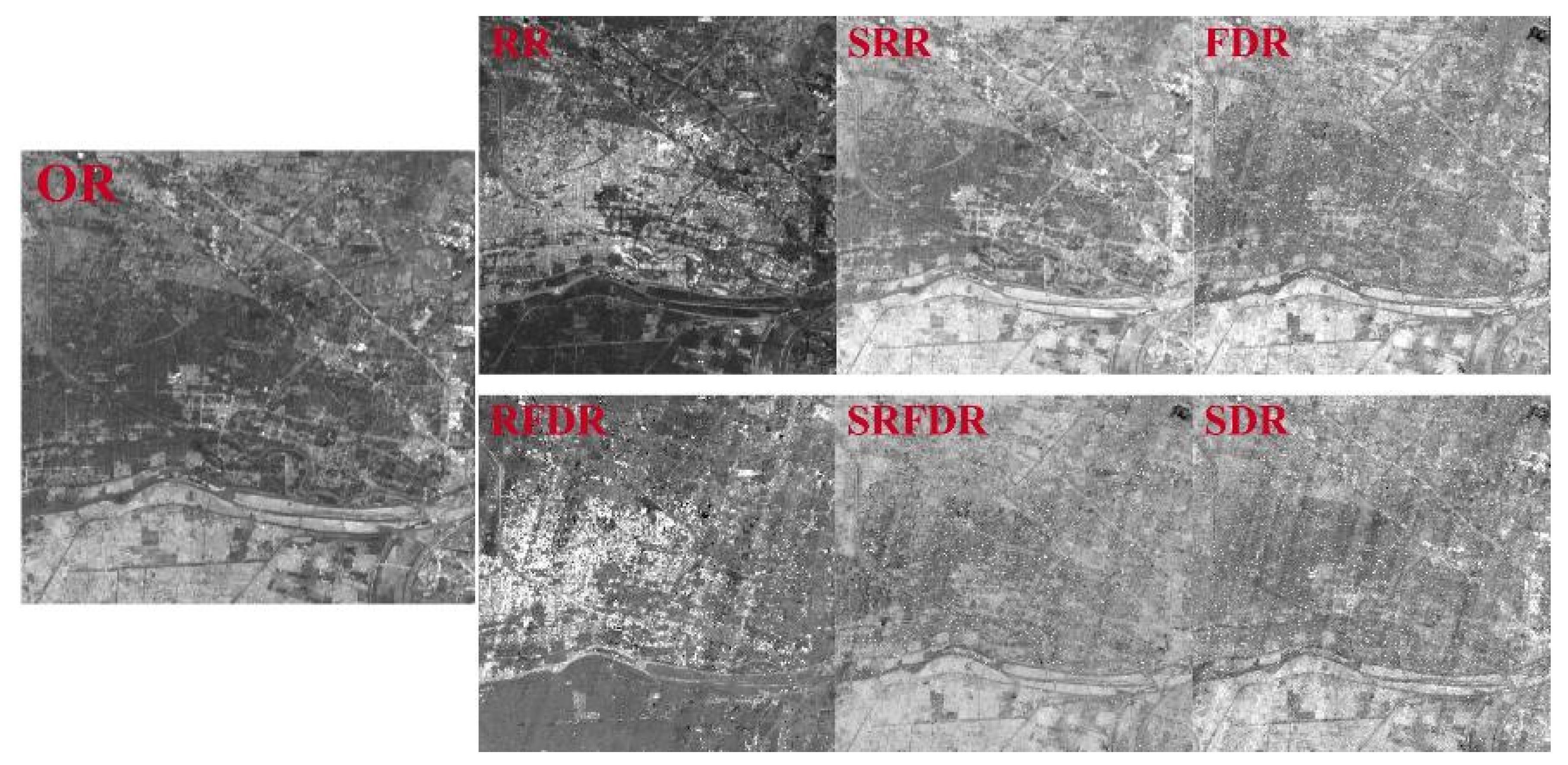
4.1. Image Quality of Transformed Spectra and SIs

Previous studies have shown that spectral transformation and index calculation of the original reflectance spectrum can improve the correlation between the spectrum and SOMC. For example, Wei et al. [7] improved the correlation between soil reflectance and SOMC by integer-order differential spectral transformations. This is also confirmed by the results of this study. As shown in Table 7, the OR of soil has no significantly correlated bands with SOMC, whereas the correlation coefficient between SDR and SOMC is greater than 0.450, which is significant at the 0.01 level.

However, the satellite imaging process is often affected by atmospheric absorption, sensor instability and other factors [62], which inevitably leads to a certain degree of noise contamination in the data (such as Gaussian noise, stripe noise [63], impulse noise, deadline noise and mixed noise) [64]. With the increase in the complexity of spectral transformation and the number of bands involved in the calculation, the uncertainty of image quality also increases. In this study, the image quality after single-band transformation, such as the reciprocal and square root, is better than after first-order differentiation. As the order of the differential transformation increases, the image quality decreases. This is mainly due to the increase in the bands involved in the calculation (as shown in Figure 10). Similar results have been reported in previous studies. For example, Wang et al. [39] found that exploiting the image spectral information by higher-order fractional derivatives was disadvantageous.

Therefore, in this study, in addition to calculating the correlation between reflectance and SOMC, the image quality of transformed reflectance was also taken into account during the construction of SIs. The bands with heavy noise were removed. In order to reduce the influence of noise on prediction results, simple SIs based on single-band spectral transformation should be used first.

In addition, this study was mainly based on the autumn AHSI/ZY1-02D data of Shuyang County. The optimal SIs obtained are suitable for the images of bare soil types of cambisols, regosols and luvisols, and the images of the rice-growing season in the Yangtze River Delta. Therefore, the application performance of the optimal SIs in different regions, vegetation growing seasons and soil types data remains to be further studied.

4.2. Advantages of Constructing SIs Separately in Bare Soil Area and Vegetation-Covered Area

Bare soil and vegetation co-exist in most cultivated land. However, the spectral response mechanisms of the two are different. Therefore, the SIs based on bare soil and vegetation-covered areas were constructed separately. In this study, the sensitive spectral wavelengths of SOM in the bare soil area are concentrated at 550–600 nm, 650–700 nm, 1100–1200 nm, 1450–1500 nm, around 2000 nm, and 2200–2300 nm (Figure 5), which are the absorption positions of soil parameters such as soil moisture, iron and SOM. These sensitive wavelengths can also explain the interaction between SOM and soil moisture and iron oxides to a certain extent. In the vegetation-covered area, the distributions of sensitive wavelengths are 500–600 nm, 700–750 nm, 1100–1300 nm, and 1900–2350 nm (Figure 6). The absorption at 1120–1200 nm and 1940–2100 nm is mainly caused by lignin, cellulose, moisture and other parameters of plants. These findings are consistent with the studies of Hong et al. [65] and Lu et al. [66]. The direct mechanism of SOM on the spectrum of bare soil pixels relies on the stretching and vibration of chemical bonds [19]. In the vegetation-covered area, SOM affects the vegetation growth, cellulose, lignin and other physicochemical parameters, and further affects the vegetation canopy spectrum. In bare soil and vegetation-covered areas, the distribution of sensitive wavelengths to SOMC is quite different, indicating the necessity of constructing SIs separately.

The |$\rho$| of the optimal SI with the highest correlation obtained in the bare soil area is 0.627 (OR-RI_(654,679)), and that in the vegetation area is 0.639 (V-RR-DSI_(551,1998)). For comparison, index construction and correlation analysis were also conducted for all sample points together. Figure 11 illustrates the correlation between SOMC and SIs constructed by different combinations of spectral transformations and index formulas. It can be seen that the highest correlation coefficient is 0.501 (p < 0.001), which is lower than the correlation coefficient of the indices constructed separately, revealing the advantage of constructing SIs separately.

4.3. The Impacts of Soil Types and Cultivated Land-Use Type on SOMC

The soil types in the cultivated land of the study area are shown in Figure 1b, and are mainly cambisols, regosols and luvisols. According to the Harmonized World Soil Database (version 1.1) provided by FAO, there was no significant difference in topsoil organic carbon content among these three types of soil. Based on the results of the distribution of SOMC levels obtained by OR-RI_(654,679) and V-RR-DSI_(551,1998) (Figure 8a), the statistical results of SOMC of different soil types are shown in

Table 10. The statistics of SOMC in different soil types.

Soil Type	Area Proportion (%)	The Minimum Value of SOMC (g/kg)	The Maximum Value of SOMC (g/kg)	Average SOMC (g/kg)
Cambisols	70.28	7.02*10−4	49.42	24.39
Regosols	9.38	0.03	45.51	24.39
Luvisols	5.67	2.61*10−3	45.44	24.05
Other soil types 1	14.68	7.16*10−3	48.75	23.41

¹ Other soil types include greyzems, anthrosols, gleysols, fluvisols, nitisols and arenosols.

. The average values of the three soil types are 24.39, 24.39 and 24.05 g/kg, respectively, and the difference among them is very small, which is consistent with previous studies [33].

The land-use types of cultivated land in the study area mainly include paddy fields, dry land and nurseries (Figure 1c). Based on the results of the distribution of SOMC levels obtained by OR-RI_(654,679) and V-RR-DSI_(551,1998) (Figure 8a), the statistical results of SOMC of different cultivated land-use types are shown in

Table 11. The statistics of SOMC in different land-use types.

Land-Use Type	The Minimum Value of SOMC (g/kg)	The Maximum Value of SOMC (g/kg)	Average SOMC (g/kg)
Paddy field	1.00*10−3	49.42	25.34
Dry land	0.02	48.75	23.23
Nursery	0.11	45.43	21.73
All	1.00*10−3	49.42	24.23

. Figure 12a–c show SOMC distribution in the paddy field, dry land and nurseries, respectively.

It can be seen from Figure 12 that the SOMC values of the three land types are all normally distributed. Overall, SOMC is the highest in paddy fields, followed by the dryland, and is lower in nurseries. In the paddy field, the SOMC is most concentrated at 25–26 g/kg. In the dryland, SOMC is most concentrated at 23–24 g/kg, whereas the SOMC in the nursery is most concentrated at 21–22 g/kg. The maximum values of SOMC distribution in the paddy field, dry land, and nursery are 49.42, 48.75, 45.43 g/kg, and the average values are 25.34, 23.23, 21.73 g/kg, respectively. There have been similar reports in previous studies. The studies of Bird et al. [67] and Huang et al. [68] showed that a low mineralization rate and the high humification coefficient of fresh organic matters in flooded soils resulted in SOC content in paddy soil that was 11–56% higher than that in dry land soil. Gao et al. [69] found that transforming paddy fields into nurseries would lead to a decrease in SOC.

West et al. [70] and Wiesmeier et al. [71] mentioned that different land-use types would significantly affect the carbon storage capacity of the soil and the distribution of SOMC, which is also confirmed in this study. The results also show that the SIs proposed in this study can effectively indicate the spatial distribution of SOMC in Shuyang County.

5. Conclusions

The AHSI data of the newly launched ZY1-02D satellite provides an important data source for soil quality monitoring. To quickly achieve an SOMC assessment on a large scale, in this study, the SOM SIs suitable for this satellite were constructed. The optimal SIs that are the most sensitive to SOMC in bare soil and vegetation-covered areas were analyzed. Moreover, the application performance of these indices was evaluated. The conclusions obtained are as follows:

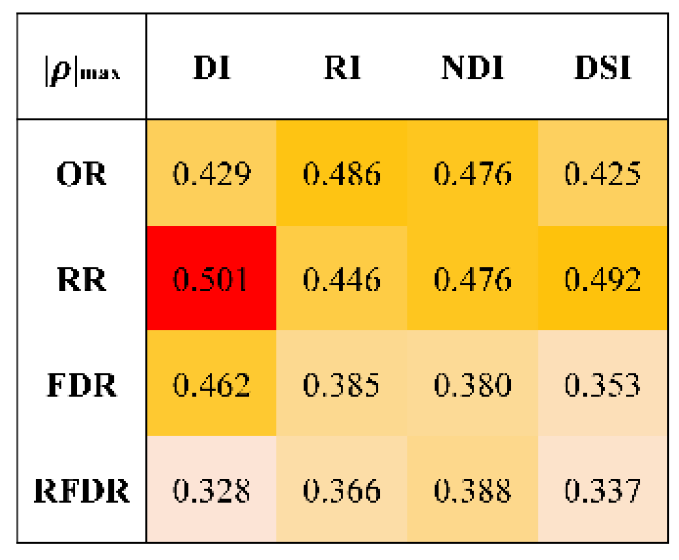
• In the bare soil area, the SIs constructed based on OR and RR have higher correlations with SOMC. For the same transformed spectrum, the SIs calculated by RI and NDI have the highest correlations with SOMC, followed by DI. Among all the constructed SIs, OR-RI_(654,679) has the highest correlation with SOMC, and the correlation coefficient is $-$0.627. In the vegetation-covered area, the correlations between SOMC and the SIs based on RR are higher than those of other transformed spectra. Among the different index formulas, the correlations between the SIs calculated by DSI and DI and SOMC are higher than those of RI and NDI. The correlation coefficient between V-RR-DSI_(551,1998) and SOMC is −0.639, which is the highest among all the calculated SIs.
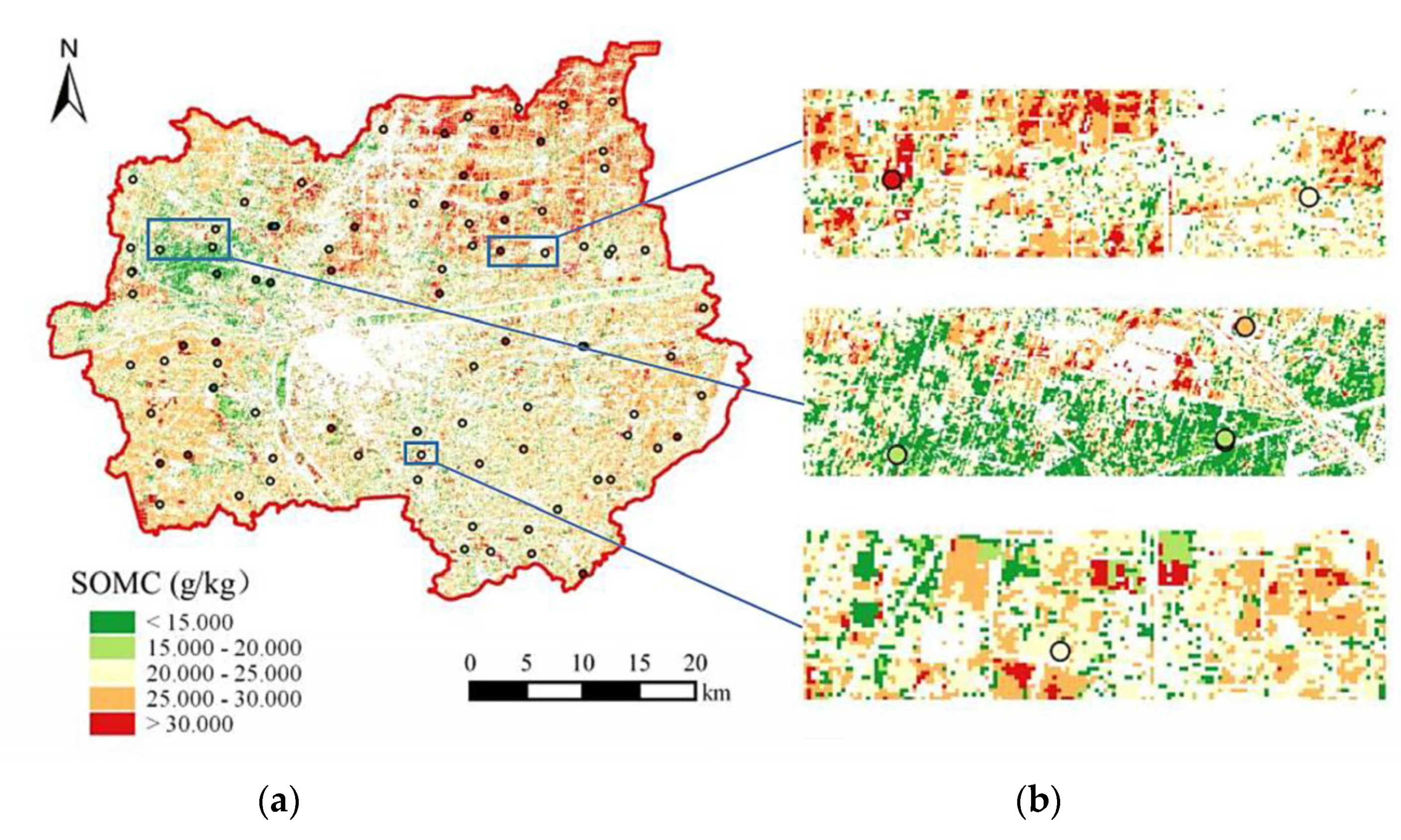
• The results show that the optimal SIs can be used to present the spatial distribution trend of SOMC and recognize SOMC levels. Based on the optimal SIs, the SOMC predicted by the model has a good linear relationship with the actual SOMC of samples. The R², RMSE and RPD of the soil-vegetation combined prediction results are 0.775, 3.72 g/kg and 2.12, respectively.

Overall, the optimal SIs constructed in this study are stable, simple to calculate, and can be used as essential parameters for SOMC estimation, showing great potential in SOMC prediction using AHSI/ZY1-02D data. In addition, the application performances of the optimal SIs in different regions, vegetation growing seasons and soil types remain to be further studied.

References

1. Luo, Z.; Wang, E.; Sun, O.J. Soil carbon change and its responses to agricultural practices in Australian agro-ecosystems: A review and synthesis. Geoderma 2010, 155, 211–223. [Google Scholar] [CrossRef]
2. Nocita, M.; Stevens, A.; van Wesemael, B.; Aitkenhead, M.; Bachmann, M.; Barthès, B.; Dor, E.B.; Brown, D.J.; Clairotte, M.; Csorba, A.; et al. Soil Spectroscopy: An Alternative to Wet Chemistry for Soil Monitoring. Adv. Agron. 2015, 132, 139–159. [Google Scholar] [CrossRef]
3. Seely, B.; Welham, C.; Blanco, J.A. Towards the application of soil organic matter as an indicator of forest ecosystem productivity: Deriving thresholds, developing monitoring systems, and evaluating practices. Ecol. Indic. 2010, 10, 999–1008. [Google Scholar] [CrossRef]
4. Six, J.; Paustian, K. Aggregate-associated soil organic matter as an ecosystem property and a measurement tool. Soil Biol. Biochem. 2014, 68, A4. [Google Scholar] [CrossRef]
5. Castaldi, F.; Palombo, A.; Santini, F.; Pascucci, S.; Pignatti, S.; Casa, R. Evaluation of the potential of the current and forthcoming multispectral and hyperspectral imagers to estimate soil texture and organic carbon. Remote Sens. Environ. 2016, 179, 54–65. [Google Scholar] [CrossRef]
6. Shi, T.; Liu, H.; Chen, Y.; Wang, J.; Wu, G. Estimation of arsenic in agricultural soils using hyperspectral vegetation indices of rice. J. Hazard. Mater. 2016, 308, 243–252. [Google Scholar] [CrossRef] [PubMed]
7. Wei, L.; Yuan, Z.; Wang, Z.; Zhao, L.; Zhang, Y.; Lu, X.; Cao, L. Hyperspectral inversion of soil organic matter content based on a combined spectral index model. Sensors 2020, 20, 2777. [Google Scholar] [CrossRef] [PubMed]
8. Rathod, P.H.; Rossiter, D.G.; Noomen, M.F.; Rathod, P.H.; Rossiter, D.G.; Noomen, M.F. Proximal Spectral Sensing to Monitor Phytoremediation of Metal-Contaminated Soils. Int. J. Phytoremediation 2013, 15, 405–426. [Google Scholar] [CrossRef] [PubMed]
9. Lagacherie, P.; Mcbratney, A.B. Spatial soil information systems and spatial soil inference systems: Perspectives for digital soil mapping. Dev. Soil Sci. 2006, 31, 3–22. [Google Scholar] [CrossRef]
10. Meng, X.; Bao, Y.; Liu, J.; Liu, H.; Zhang, X.; Zhang, Y.; Wang, P.; Tang, H.; Kong, F. Regional soil organic carbon prediction model based on a discrete wavelet analysis of hyperspectral satellite data. Int. J. Appl. Earth Obs. Geoinf. 2020, 89, 102111. [Google Scholar] [CrossRef]
11. Shang, K.; Xiao, C.; Gan, F.; Wei, H. Estimation of soil copper content in mining area using ZY1-02D satellite hyperspectral data. J. Appl. Remote Sens. 2021, 15, 042607. [Google Scholar] [CrossRef]
12. Wang, J.; He, T.; Lv, C.; Chen, Y.; Jian, W. Mapping soil organic matter based on land degradation spectral response units using Hyperion images. Int. J. Appl. Earth Obs. Geoinf. 2010, 12, S171–S180. [Google Scholar] [CrossRef]
13. Tiwari, S.K.; Saha, S.K.; Kumar, S. Prediction Modeling and Mapping of Soil Carbon Content Using Artificial Neural Network, Hyperspectral Satellite Data and Field Spectroscopy. Adv. Remote Sens. 2015, 4, 63–72. [Google Scholar] [CrossRef] [Green Version]
14. Emadi, M.; Taghizadeh-Mehrjardi, R.; Cherati, A.; Danesh, M.; Mosavi, A.; Scholten, T. Predicting and mapping of soil organic carbon using machine learning algorithms in Northern Iran. Remote Sens. 2020, 12, 2234. [Google Scholar] [CrossRef]
15. FAO Soil Organic Carbon Mapping Cookbook; FAO: Rome, Italy, 2017; ISBN 9789251304402.
16. Venter, Z.S.; Hawkins, H.J.; Cramer, M.D.; Mills, A.J. Mapping soil organic carbon stocks and trends with satellite-driven high resolution maps over South Africa. Sci. Total Environ. 2021, 771, 145384. [Google Scholar] [CrossRef] [PubMed]
17. Donlon, C.J.; Cullen, R.; Giulicchi, L.; Vuilleumier, P.; Francis, C.R.; Kuschnerus, M.; Simpson, W.; Bouridah, A.; Caleno, M.; Bertoni, R.; et al. The Copernicus Sentinel-6 mission: Enhanced continuity of satellite sea level measurements from space. Remote Sens. Environ. 2021, 258, 112395. [Google Scholar] [CrossRef]
18. Arthur Endsley, K.; Kimball, J.S.; Reichle, R.H.; Watts, J.D. Satellite Monitoring of Global Surface Soil Organic Carbon Dynamics Using the SMAP Level 4 Carbon Product. J. Geophys. Res. Biogeosci. 2020, 125, 1–18. [Google Scholar] [CrossRef]
19. Clark, R.N.; King, T.V.V.; Klejwa, M.; Swayze, G.A. High Spectral Resolution Reflectance Spectroscopy of Minerals. J. Geophys. Res. Solid Earth 1990, 95, 12653–12680. [Google Scholar] [CrossRef] [Green Version]
20. Ben-dor, E. Near-Infrared Analysis as a Rapid Method to Simultaneously Evaluate Several Soil Properties. Soil Sci. Soc. Am. J. 1995, 59, 364–372. [Google Scholar] [CrossRef]
21. Krishnan, P.; Alexander, J.D.; Butler, B.J.; Hummel, J.W. Reflectance Technique for Predicting Soil Organic Matter. Soil Sci. Soc. Am. J. 1980, 44, 1282–1285. [Google Scholar] [CrossRef]
22. Bartholomeus, H.M.; Schaepman, M.E.; Kooistra, L.; Stevens, A.; Hoogmoed, W.B.; Spaargaren, O.S.P. Spectral reflectance based indices for soil organic carbon quantification. Geoderma 2008, 145, 28–36. [Google Scholar] [CrossRef]
23. Jin, X.; Du, J.; Liu, H.; Wang, Z.; Song, K. Remote estimation of soil organic matter content in the Sanjiang Plain, Northest China: The optimal band algorithm versus the GRA-ANN model. Agric. For. Meteorol. 2016, 218, 250–260. [Google Scholar] [CrossRef]
24. Prescott, C.E.; Maynard, D.G.; Laiho, R. Humus in northern forests: Friend or foe? For. Ecol. Manage. 2000, 133, 23–36. [Google Scholar] [CrossRef]
25. Munson, S.A.; Carey, A.E. Organic matter sources and transport in an agriculturally dominated temperate watershed. Appl. Geochem. 2004, 19, 1111–1121. [Google Scholar] [CrossRef]
26. Zhang, Y.; Guo, L.; Chen, Y.; Shi, T.; Luo, M.; Ju, Q.L.; Zhang, H.; Wang, S. Prediction of soil organic carbon based on Landsat 8 monthly NDVI data for the Jianghan Plain in Hubei Province, China. Remote Sens. 2019, 11, 1683. [Google Scholar] [CrossRef] [Green Version]
27. Takata, Y. Analysis of spatial and temporal variation of soil organic carbon budget in northern Kazakhstan. Jpn. Agric. Res. Q. 2010, 44, 335–342. [Google Scholar] [CrossRef] [Green Version]
28. Zhao, M.S.; Rossiter, D.G.; Li, D.C.; Zhao, Y.G.; Liu, F.; Zhang, G.L. Mapping soil organic matter in low-relief areas based on land surface diurnal temperature difference and a vegetation index. Ecol. Indic. 2014, 39, 120–133. [Google Scholar] [CrossRef]
29. Kumar, P.; Pandey, P.C.; Singh, B.K.; Katiyar, S.; Mandal, V.P.; Rani, M.; Tomar, V.; Patairiya, S. Estimation of accumulated soil organic carbon stock in tropical forest using geospatial strategy. Egypt. J. Remote Sens. Sp. Sci. 2016, 19, 109–123. [Google Scholar] [CrossRef] [Green Version]
30. Shuyang-Meteorological Data-China Weather Network. Available online: http://www.weather.com.cn/cityintro/101191302.shtml (accessed on 19 January 2022).
31. Zeng, Y.; Guo, H.; Yao, Y.; Huang, L. The formation of agricultural e-commerce clusters: A case from China. Growth Chang. 2019, 50, 1356–1374. [Google Scholar] [CrossRef]
32. Yang, S.C.; Huang, Z.M.; Huang, C.Y.; Tsai, C.C.; Yeh, T.K. A case study on the impact of ensemble data assimilation with GNSS-zenith total delay and radar data on heavy rainfall prediction. Mon. Weather Rev. 2020, 148, 1075–1098. [Google Scholar] [CrossRef]
33. Hamonized World Soil Database (Version 1.1). Available online: https://geodata.pku.edu.cn/index.php?c=content&a=show&id=730# (accessed on 19 January 2022).
34. Shi, X.; Yu, D.; Sun, W.; Wang, H.; Zhao, Q.; Gong, Z. Reference benchmarks relating to great groups of genetic soil classification of China with soil taxonomy. Chin. Sci. Bull. 2004, 49, 1507–1511. [Google Scholar] [CrossRef]
35. Xin, Z.; Huang, B.; Dong, C.S.; Weixia, S.; Hu, W.Y.; Tian, K. Tempo-spatial variability of soil organic matter and total nitrogen in farmland and its affecting factors in Shuyang county, Jiangsu province. Soils 2013, 45, 405–411. [Google Scholar] [CrossRef]
36. Press, W.H.; Teukolsky, S.A. Savitzky-Golay Smoothing Filters. Comput. Phys. 1990, 4, 669. [Google Scholar] [CrossRef]
37. Gitelson, A.; Merzlyak, M.N. Spectral reflectance changes associated with autumn senescence of Aesculus hippocastanum L. and Acer platanoides L. leaves. Spectral features and relation to chlorophyll estimation. J. Plant Physiol. 1994, 143, 286–292. [Google Scholar] [CrossRef]
38. Sims, D.A.; Gamon, J.A. Relationships between leaf pigment content and spectral reflectance across a wide range of species, leaf structures and developmental stages. Remote Sens. Environ. 2002, 81, 337–354. [Google Scholar] [CrossRef]
39. Wang, X.; Zhang, F.; Kung, H.T.; Johnson, V.C. New methods for improving the remote sensing estimation of soil organic matter content (SOMC) in the Ebinur Lake Wetland National Nature Reserve (ELWNNR) in northwest China. Remote Sens. Environ. 2018, 218, 104–118. [Google Scholar] [CrossRef]
40. Chen, H.; Pan, T.; Chen, J.; Lu, Q. Waveband selection for NIR spectroscopy analysis of soil organic matter based on SG smoothing and MWPLS methods. Chemom. Intell. Lab. Syst. 2011, 107, 139–146. [Google Scholar] [CrossRef]
41. Larney, F.J.; Ellert, B.H.; Olson, A.F. Carbon, ash and organic matter relationships for feedlot manures and composts. Can. J. Soil Sci. 2005, 85, 261–264. [Google Scholar] [CrossRef]
42. Lu, Q.; Wang, S.; Bai, X.; Liu, F.; Tian, S.; Wang, M.; Wang, J. Rapid estimation of soil heavy metal nickel content based on optimized screening of near-infrared spectral bands. Acta Geochim. 2020, 39, 116–126. [Google Scholar] [CrossRef]
43. Ben-Dor, E.; Inbar, Y.; Chen, Y. The reflectance spectra of organic matter in the visible near-infrared and short wave infrared region (400-2500 nm) during a controlled decomposition process. Remote Sens. Environ. 1997, 61, 1–15. [Google Scholar] [CrossRef]
44. Edward, M. Barnes, Kenneth A. Sudduth, John W. Hummel, Scott M. Lesch, D.L.C.; Chenghai Yang, Craig S.T. Daughtry, and W.C.B. Remote- and Ground-Based Sensor Techniques to Map Soil Properties. Commun. Soil Sci. Plant Anal. 2015, 46, 1668–1676. [Google Scholar] [CrossRef]
45. Ladoni, M.; Alaviph, S.K.A.; Bahrami, H.A.; Noroozi, A.A. Remote sensing of soil organic carbon in semi-arid region of iran. Arid L. Res. Manag. 2010, 24, 271–281. [Google Scholar] [CrossRef]
46. Yadav, J.; Sehra, K. Large Scale Dual Tree Complex Wavelet Transform based robust features in PCA and SVD subspace for digital image watermarking. Procedia Comput. Sci. 2018, 132, 863–872. [Google Scholar] [CrossRef]
47. George, J.; Kumar, S. Hyperspectral Remote Sensing in Characterizing Soil Salinity Severity using SVM Technique—A Case Study of Alluvial Plains. Int. J. Adv. Remote. Sens. GIS 2015, 4, 1344–1360. [Google Scholar] [CrossRef] [Green Version]
48. Meng, X.; Bao, Y.; Ye, Q.; Liu, H.; Zhang, X.; Tang, H.; Zhang, X. Soil organic matter prediction model with satellite hyperspectral image based on optimized denoising method. Remote Sens. 2021, 13, 2273. [Google Scholar] [CrossRef]
49. Yuan, J.; Wang, X.; Yan, C.X.; Wang, S.R.; Ju, X.P.; Li, Y. Soil moisture retrieval model for remote sensing using reflected hyperspectral information. Remote Sens. 2019, 11, 366. [Google Scholar] [CrossRef] [Green Version]
50. Haubrock, S.N.; Chabrillat, S.; Lemmnitz, C.; Kaufmann, H. Surface soil moisture quantification models from reflectance data under field conditions. Int. J. Remote Sens. 2008, 29, 3–29. [Google Scholar] [CrossRef]
51. Nocita, M.; Stevens, A.; Noon, C.; Van Wesemael, B. Prediction of soil organic carbon for different levels of soil moisture using Vis-NIR spectroscopy. Geoderma 2013, 199, 37–42. [Google Scholar] [CrossRef]
52. Daughtry, C.S.T. Agroclimatology: Discriminating crop residues from soil by shortwave infrared reflectance. Agron. J. 2001, 93, 125–131. [Google Scholar] [CrossRef]
53. Bartholomeusa, H. Quantitative retrieval of soil organic carbon using laboratory spectroscopy and spectral indices. In Proceedings of the ISPRS Commission VII Symposium ‘Remote Sensing: From Pixels to Processes’, Enschede, The Netherlands, 8–11 May 2006. [Google Scholar]
54. Daughtry, C.S.T.; Hunt, E.R.; McMurtrey, J.E. Assessing crop residue cover using shortwave infrared reflectance. Remote Sens. Environ. 2004, 90, 126–134. [Google Scholar] [CrossRef]
55. Fourty, T.; Baret, F.; Jacquemoud, S.; Schmuck, G.; Verdebout, J. Leaf optical properties with explicit description of its biochemical composition: Direct and inverse problems. Remote Sens. Environ. 1996, 56, 104–117. [Google Scholar] [CrossRef]
56. Melillo, J.M.; Aber, J.D.; Muratore, J.F.; Jun, N. Nitrogen and Lignin Control of Hardwood Leaf Litter Decomposition Dynamics. Ecology 2008, 63, 621–626. [Google Scholar] [CrossRef]
57. Serrano, L.; Peñuelas, J.; Ustin, S.L. Remote sensing of nitrogen and lignin in Mediterranean vegetation from AVIRIS data. Remote Sens. Environ. 2002, 81, 355–364. [Google Scholar] [CrossRef]
58. Wang, K.; Qi, Y.; Guo, W.; Zhang, J.; Chang, Q. Retrieval and mapping of soil organic carbon using sentinel-2A spectral images from bare cropland in autumn. Remote Sens. 2021, 13, 1072. [Google Scholar] [CrossRef]
59. Welikhe, P.; Quansah, J.E.; Fall, S.; McElhenney, W. Estimation of Soil Moisture Percentage Using LANDSAT-based Moisture Stress Index. J. Remote Sens. GIS 2017, 6, 1–5. [Google Scholar] [CrossRef]
60. Marsett, R.C.; Qi, J.; Heilman, P.; Biedenbender, S.H.; Watson, M.C.; Amer, S.; Weltz, M.; Goodrich, D.; Marsett, R. Remote sensing for grassland management in the arid Southwest. Rangel. Ecol. Manag. 2006, 59, 530–540. [Google Scholar] [CrossRef]
61. Guo, P.; Li, T.; Gao, H.; Chen, X.; Cui, Y. Evaluating Calibration and Spectral Variable Selection Methods for Predicting Three Soil Nutrients Using Vis-NIR Spectroscopy. Remote Sens. 2021, 13, 4000. [Google Scholar] [CrossRef]
62. Zhang, Q.; Yuan, Q.; Li, J.; Liu, X.; Shen, H.; Zhang, L. Hybrid noise removal in hyperspectral imagery with a spatial-spectral gradient network. IEEE Trans. Geosci. Remote Sens. 2019, 57, 7317–7329. [Google Scholar] [CrossRef]
63. Li, C.; Zhou, C.; Ma, L.; Tang, L.; Wang, X. A stripe noise removal method of interference hyperspectral imagery based on interferogram correction. Image Signal Process. Remote Sens. XVIII 2012, 8537, 85370A. [Google Scholar] [CrossRef]
64. Rasti, B.; Scheunders, P.; Ghamisi, P.; Licciardi, G.; Chanussot, J. Noise reduction in hyperspectral imagery: Overview and application. Remote Sens. 2018, 10, 482. [Google Scholar] [CrossRef] [Green Version]
65. Hong, Y.; Yu, L.; Chen, Y.; Liu, Y.; Liu, Y.; Liu, Y.; Cheng, H. Prediction of soil organic matter by VIS-NIR spectroscopy using normalized soil moisture index as a proxy of soil moisture. Remote Sens. 2018, 10, 28. [Google Scholar] [CrossRef] [Green Version]
66. Lu, Y.; Bai, Y.; Yang, L.; Wang, H. Hyperspectral extraction of soil organic matter content based on principal component regression. N. Z. J. Agric. Res. 2007, 50, 1169–1175. [Google Scholar] [CrossRef]
67. Bird, J.A.; Van Kessel, C.; Horwath, W.R. Stabilization of 13C-Carbon and Immobilization of 15N-Nitrogen from Rice Straw in Humic Fractions. Soil Sci. Soc. Am. J. 2003, 67, 806–816. [Google Scholar] [CrossRef]
68. Huang, R.; Lan, M.; Liu, J.; Gao, M. Soil aggregate and organic carbon distribution at dry land soil and paddy soil: The role of different straws returning. Environ. Sci. Pollut. Res. 2017, 24, 27942–27952. [Google Scholar] [CrossRef] [PubMed]
69. Gao, J.; Pan, G.; Jiang, X.; Pan, J.; Zhuang, D. Land-use induced changes in topsoil organic carbon stock of paddy fields using MODIS and TM / ETM analysis: A case study of Wujiang County, China. J. Environ. Sci. 2008, 20, 852–858. [Google Scholar] [CrossRef]
70. West, T.O.; Marland, G. A synthesis of carbon sequestration, carbon emissions, and net carbon flux in agriculture: Comparing tillage practices in the United States. Agric. Ecosyst. Environ. 2008, 91, 217–232. [Google Scholar] [CrossRef]
71. Wiesmeier, M.; Von Lützow, M.; Spörlein, P.; Geuß, U.; Hangen, E.; Reischl, A.; Schilling, B.; Kögel-knabner, I. Land use effects on organic carbon storage in soils of Bavaria: The importance of soil types. Soil Tillage Res. 2015, 146, 296–302. [Google Scholar] [CrossRef]
Figure 1. Overview of the study area and sampling points: (a) location, (b) soil types, and (c) land-use types.
Ijgi 11 00111 g001
Figure 2. (a) The true-color satellite image (R: 662 nm, G: 551 nm, B: 482 nm) of Advanced Hyperspectral Imager (AHSI) data of ZY1-02D satellite obtained on 22 October 2020, in Shuyang County, (b) the schemata the for five-point method, (c) distribution of bare soil and vegetation-covered areas.
Ijgi 11 00111 g002
Figure 3. Flowchart of the research.
Ijgi 11 00111 g003
Figure 4. The reflectance spectra of soil samples with different soil organic matter content (SOMC) in (a) bare soil and (b) vegetation-covered area.
Ijgi 11 00111 g004
Figure 5. Correlation coefficient matrix of spectral indices (SIs) and SOMC of soil samples in the bare soil area.
Ijgi 11 00111 g005
Figure 6. Correlation coefficient matrix of SIs and SOMC of soil samples in the vegetation-covered area.
Ijgi 11 00111 g006
Figure 7. The correlations of SOMC and different SIs.
Ijgi 11 00111 g007
Figure 8. (a) Recognition of SOMC levels in soil samples in cultivated land area of Shuyang County and (b) details of partial enlargement.
Ijgi 11 00111 g008
Figure 9. The prediction accuracy of SOMC in the cultivated land of Shuyang County.
Ijgi 11 00111 g009
Figure 10. Reflectance images after different spectral transformations at 645 nm (from the AHSI/ZY1-02D data). The meanings of OR, RR, SRR, FDR, RFDR, SRFDR and SDR are consistent with Table 2.
Ijgi 11 00111 g010
Figure 11. The maximum correlation coefficient between SOMC of SIs constructed by different combinations of spectral transformations and index formulas.
Ijgi 11 00111 g011
Figure 12. Distribution of SOMC in different land-use types ((a) paddy field, (b) dry land and (c) nursery) in Shuyang County.
Ijgi 11 00111 g012