Downscaling of AMSR-E Soil Moisture over North China Using Random Forest Regression

Abstract

Satellite retrieval can offer global soil moisture information, such as Advanced Microwave Scanning Radiometer-Earth Observing System (AMSR-E) data. AMSR-E has been used to provide soil moisture all over the world, with a coarse resolution of 25 km × 25 km. The coarse resolution of the soil moisture dataset often hinders its use in local or regional research. This work proposes a new framework based on the random forest (RF) model while using five auxiliary data to downscale the AMSR-E soil moisture data over North China. The downscaled results with a 1 km spatial resolution are verified against in situ measurements. Compared with AMSR-E data, the correlation coefficient of the downscaled data is increased by 0.17, and the root mean squared error, mean absolute error, and unbiased root mean square error are reduced by 0.02, 0.01, and 0.03 m³/m³, respectively. In addition, the comparison results with Multiple Linear Regression and Support Vector Regression downscaled data show that the proposed method significantly outperforms the other two methods. The feasibility of our model is well supported by the importance analysis and leave-one-out analysis. Our study, which combines RF with spatiotemporal search algorithms and efficient auxiliary data, may provide insights into soil moisture downscaling in large areas with various surface characteristics and climatic conditions.

1. Introduction

Soil moisture plays a considerable part in the process of global water and energy balance [1], affecting many fields, such as hydrology, meteorology, and agriculture. The characteristics of soil moisture change can reflect many physical and chemical properties of soil, and soil moisture also has a significant impact on terrestrial ecosystems. Nowadays, soil moisture monitoring has been widely used in drought monitoring [2,3], water resources assessment [4,5], crop yield estimation [6], weather forecasting, and hydrological simulation [7,8]. Therefore, obtaining accurate and high-resolution soil moisture data is of great significance for ecosystem balance research and coping with climate change [9,10].

In the past few years, drought disasters in North China have been increasing and have become one of the most serious natural disasters. The rapid growth of industrial, irrigation, and domestic water consumption has led to a sharp increase in water resource consumption, which in turn has led to more serious droughts in northern China [11]. It is significantly urgent to improve our understanding of the spatial and temporal variations of soil moisture and quantify the drought situation. However, research on soil moisture downscaling in northern China is inadequate. Therefore, it is necessary to establish a set of regional soil moisture data with high spatial resolution in North China.

In recent years, the development of remote sensing technology has provided convenience for the acquisition of soil moisture [12]. At the same time, microwave remote sensor is a reliable method to estimate soil moisture (SM) [13], as the microwave is very sensitive to SM changes, less affected by different weather conditions [14], and can realize all-weather and all-coverage Earth observations. At present, a variety of satellite soil moisture products are available, such as Advanced Microwave Scanning Radiometer-Earth Observing System (AMSR-E) [15], Soil Moisture Active Passive (SMAP) [16], and Soil Moisture and Ocean Salinity (SMOS) [17]. The SM data provided by these products is efficient in some large-scale applications [18]. However, for small-scale research, the spatial resolution of these products is too coarse, basically tens of kilometers [19,20], which is not adequate for capturing the spatial heterogeneity of SM. Therefore, these products are very limited in some regional- and local-scale research [21]. Meanwhile, the 1-km spatial resolution has become a common high resolution in many SM downscaling studies [22].

To solve the problem of the rough spatial resolution of satellite remote sensing data, plenty of methods have been presented to improve their resolution. At present, the research focused on downscaling methods and applications can be roughly divided into the following three categories: (1) model-based methods [23], (2) methods based on multi-source satellite remote sensing data fusion [24], and (3) methods using geo-information data [22,25]. Each category can be subdivided into several categories according to specific conditions. Model-based methods are divided into statistical models [26] and land surface models. Based on the land surface models, there are deterministic downscaling [27], statistical downscaling [28], and data assimilation [29]. No matter what kind of model-based method, we need to consider whether the model can be applied to a wider range of research. Furthermore, the model needs a lot of input parameter data, and obtaining this data is difficult, which makes the application have many limitations. The methods based on multi-source satellite data fusion are divided into two methods according to the different fusion data: the fusion method of active and passive microwave data [30] and the fusion method of optical/thermal and microwave data [31]. Earlier scholars have made a lot of attempts and found that the combination of active and passive microwave remote sensing data can obtain more accurate results. Nevertheless, the active microwave data is expensive and needs detailed terrain, vegetation, and other information, so it is a challenge to use and popularize it on a large scale [30]. The downscaling methods using geo-information data are mainly based on the spatial distribution relationship between soil moisture and other land surface variables, such as terrain, soil attributes, and vegetation characteristics [32]. On this basis, the geo-statistical or fractal interpolation model is constructed. In this method, terrain is often used as an auxiliary information source [33]. This method can infer fine-scale changes in soil moisture from the relationship between soil moisture and available auxiliary variables. However, when establishing geo-statistical or analytical interpolation models, a large number of in situ observations need to be used. At the same time, these models have obvious regional characteristics, which obviously limit their applicability [25].

With the improvement of computer performance and the development of artificial intelligence technology, machine learning methods have been introduced into the study of soil moisture downscaling. Machine learning is a kind of data analysis method, which enables computers to learn from data intelligently to find hidden patterns of phenomena [1]. Many studies have shown that compared with other machine learning methods, the random forest (RF) algorithm is more suitable for satellite product downscaling [34,35]. Since the RF model can describe nonlinear correlation and adopt the ensemble method, it becomes more flexible through randomization. At the same time, this method does not require many in situ data to participate in the model. Although the RF model requires some high-resolution auxiliary data, these data are relatively easy to obtain. However, the application of RF in large areas is insufficient, and RF is also very sensitive to surface characteristics and driving parameters, especially in arid and semi-arid areas.

Based on the above issues, this study explores how the random forest method works under large-scale and complex conditions combined with effective parameters. The purpose of our study was to propose 1 efficient method to downscale the soil moisture data of AMSR-E over North China from 25 to 1 km. Our study combines RF with spatiotemporal search algorithms and the effective auxiliary data, which is easy to obtain and relate to soil moisture. We evaluated the downscaled results with in situ observations. The proposed downscaling method was furthermore compared with other commonly used downscaling methods and several methods of earlier studies. Section 2 details the methods and data used in this paper. The results of the study are described in Section 3. The discussion part is given in Section 4. The discussion section provides the importance analysis of explanatory factors, leave-one-out analysis, comparison of different methods, and limitations of the study. The conclusion is given at the end of the article (Section 5).

2. Materials and Methods

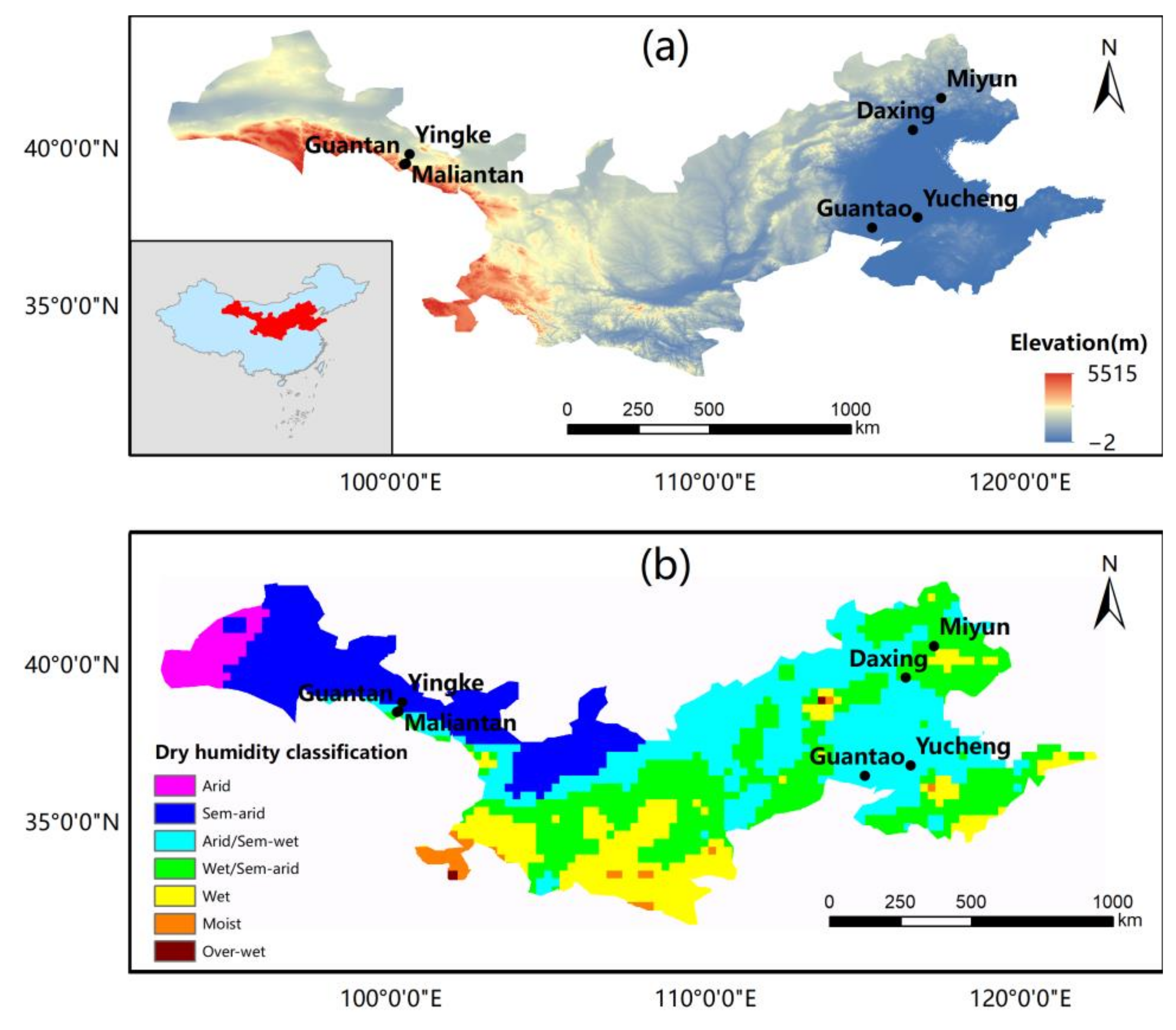
2.1. Study Area

Figure 1 shows the elevation and dry humidity classification map of the study area. The location of the selected ground stations in this study is also shown in the figure. The study area is North China, between longitude 32° N and 42° N and latitude 93° E and 123° E, with an area of about 14,900 km². It includes Shandong, Hebei, Ningxia, Gansu, Shanxi, Shaanxi, Beijing, and Tianjin. The climate zone in this region has a large span, including temperate monsoon climate, subtropical monsoon climate, plateau mountain climate, temperate continental climate, warm temperate semi-humid and semi-arid monsoon climate, etc. The land use types are complex, with about 18 land use types. The altitude of this area ranges from −2 to 5516 m.

2.2. Study Data

The spatial downscaling process of soil moisture data based on passive microwave satellite remote sensing data must be supported by the image information of relevant surface features. The image information is provided by the data with higher spatial resolution. In this study, the Moderate Resolution Imaging Spectroradiometer (MODIS), DEM, and precipitation data with higher spatial resolution were used to support the spatial downscaling based on AMSR-E data. At the same time, the ground station data was selected to verify the results. The data used in this study, its specific description, and spatial resolution are shown in

Table 1. List of remote sensing soil moisture data and auxiliary data used in this study.

Datasets	Description	Spatiotemporal Resolution
LPRM-AMSR_E	Soil moisture (SM)	25 km/daily
MOD11A1	Land surface temperature (LST)	1 km/daily
MOD13A2	Normalized difference vegetation index (NDVI)	1 km/16 d
MCD43C3	Surface albedo (ALB)	0.05°/daily
SRTM DEM	Elevation	90 m/-
prec_ITPCAS-CMFD	Precipitation	0.1°/daily

.

2.2.1. AMSR-E Soil Moisture Data

AMSR-E was developed by the National Aeronautics and Space Administration (NASA) and the Japan Aerospace Exploration Agency (JAXA). AMSR-E was carried on the Aqua polar orbit of NASA Earth Observation System (EOS) and launched in May 2002. AMSR-E measures the brightness temperature of vertical and horizontal polarization at 6 frequencies of 6.9, 10.7, 18.7, 23.8, 36.5, and 89.0 GHz.

In this study, level 3 soil moisture data of AMSR-E in 2009 were selected and developed based on the Land Parameter Retrieval Model (LPRM), with a spatial resolution of 25 km [36]. The product was available free of charge from NASA’s official website (http://search.earthdata.nasa.uov/search, 19 November 2020).

2.2.2. MODIS Data

Vegetation index, Albedo, and land surface temperature have been extensively used in the downscaling of remote sensing soil moisture data in many studies [37,38]. These parameters are available from Moderate Resolution Imaging Spectroradiometer (MODIS). MODIS on Terra and Aqua satellites is a large space remote sensing instrument developed by NASA. At present, it has been widely used for monitoring various environments, including ocean, land surface, and so on. In this study, three MODIS products were used, including the normalized difference vegetation index (NDVI), land surface temperature (LST), and Albedo.

LST was obtained from MODIS daily product MOD11A1, and NDVI was acquired from 16 day vegetation index product MOD13A2. The spatial resolution of both is 1 km. The Albedo was obtained from the daily Albedo product MCD43C3 with a resolution of 0.05°. These data were acquired from the Land Process Distributed Active Archive Center (LP DAAC) (https://lpdaac.usgs.gov/, 30 April 2021).

2.2.3. DEM

In many studies of soil moisture downscaling, elevation is considered to be one of the most effective topographical features [39,40]. Therefore, we used this variable to downscale the AMSR-E SM data in our proposed approach.

Digital elevation model (DEM) data was acquired from NASA’s Space Shuttle Radar Topography Mission (SRTM). The data has a spatial resolution of 90 m and is one of the most used DEM data.

2.2.4. Precipitation Data

The most direct way for the atmosphere to affect land soil moisture is through precipitation [41]. Many regional- and global-scale studies have confirmed the tele-connection between precipitation and soil moisture variability [42].

The precipitation data is the China meteorological forcing dataset (CMFD) from the national Qinghai Tibet Plateau science data center, which is a set of near land surface meteorological reanalysis data. CMFD is made with the Princeton reanalysis data, GEWEX-SRB radiation data, GLDAS and TRMM precipitation data as the background field, and the conventional meteorological observation data [43,44]. The data set was provided by the National Tibetan Plateau Data Center (http://data.tpdc.ac.cn, 20 April 2021).

2.2.5. In Situ Soil Moisture Observations

To evaluate the accuracy of downscaled soil moisture, field measurement data from 7 locations in 2009 were collected. Field measurements at seven sites were obtained from the Chinese Ecosystem Research Network (CERN) and the Watershed Allied Telemetry Experimental Research (WATER) project. The data set was provided by the National Tibetan Plateau Data Center (http://data.tpdc.ac.cn, 26 April 2021). Each site was equipped with a set of quadratic net radiometers (CNR1 and CNR4) that collected atmospheric down-welling and up-welling longwave radiation. In total, 6 layers of soil moisture sensors were arranged at depths of 0.05, 0.1, 0.20, 0.40, 0.80, and 1.20 m, respectively. Detailed information of the 7 sites is exhibited in

Table 2. Information of the field sites.

ID	Site	Land-Cover	Elevation	Longitude	Latitude
1	Guantan	Forest	2835 m	100.25 E	38.53 N
2	Maliantan	Grassland	2817 m	100.30 E	38.55 N
3	Yingke	Cropland	1519 m	100.42 E	38.85 N
4	Daxing	Cropland	20 m	116.42 E	39.62 N
5	Guantao	Cropland	30 m	115.12 E	36.51 N
6	Miyun	Orchard	350 m	117.32 E	40.63 N
7	Yucheng	Cropland	23 m	116.57 E	36.83 N

.

2.3. Methods

2.3.1. Random Forest Model

The RF model [45] is an improved decision tree model, which makes decisions by averaging multiple regression trees [46]. The model is nonlinear and insensitive to outliers. Compared with other machine learning methods, the RF model is more widely used in the downscaling of SM data [47]. The major idea of the RF model is to build the nonlinear function relationship between various input parameters and output soil moisture:

$$\mathrm{SM}=f_{RF}\left(\mathrm{C}\right)+\mathsf{\epsilon }$$

(1)

where the left SM is soil moisture data, and C is an input vector representing various input parameters; $f_{RF}$ is the nonlinear function that establishes the relationship between input parameters and output SM.

RF establishes several decision trees in the training stage, and then calculates the average prediction value of these trees as the output of the method. RF models can divide the input feature space into a lot of regression trees, called a forest, in which each tree is generated by guided samples. One boot sample contains approximately two-thirds of the training samples, and one-third of the remaining data is used to validate each tree. The result of RF is the average prediction result of each decision tree, as follows:

$$f\left(SM|C\right)=\frac{1}{n}{{\displaystyle \sum }}_{i=1}^n{f}_i(SM|C)$$

(2)

where n is the number of regression trees, $f\left(SM|C\right)$ is the ensemble decision tree, and $f_i(SM|C)$ is the sub-decision tree of the original soil moisture $\left(SM\right)$ given the bootstrapped data from the training input variables $\left(C\right)$.

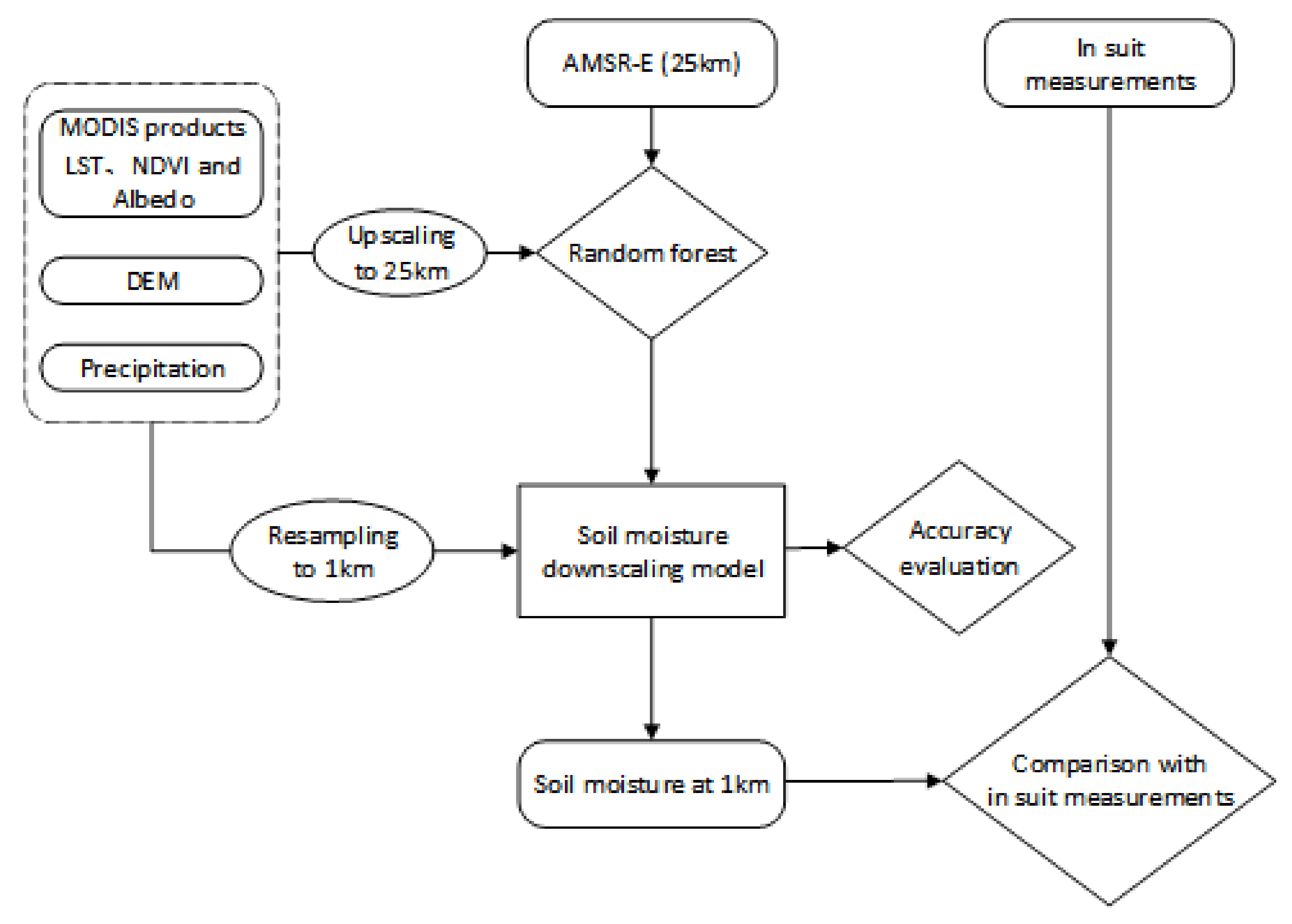
2.3.2. Soil Moisture Downscaling Framework

In order to downscale AMSR-E soil moisture data, we used known high-resolution data sets closely related to soil moisture, including LST, NDVI, Albedo, DEM, and precipitation. Atmospheric auxiliary variables (LST, Albedo, and precipitation) can maintain the temporal variations of the downscaled SM. The geophysical auxiliary variable DEM is used to capture the spatial variations and patterns of the downscaled SM. The other auxiliary variable, such as NDVI, is also included to illustrate the impact of vegetation variations on the spatiotemporal pattern of the downscaled SM.

In this study, we used the RF models to develop a downscaling framework. The foundation of this method is explained in detail in the Section 2.3.1. The major contribution of this study is to propose a new method that incorporates the above five effective auxiliary data into the RF models to improve the estimation of soil moisture at a finer resolution.

A reliable spatial and temporal window size is the basis of the success of the presented method, as too large of a window may lead to over-fitting problems in the regression model. In this study, we used an adaptive spatiotemporal window size determination method. Two key parameters are used to decide the window size: the temporal day number and the spatial window size. The initial value of the spatial window size needs to be given first. When the corresponding conditions are met, the model will automatically search until termination. More details regarding this strategy can be found in our previous studies [48].

Figure 2 shows the process of the proposed method. The following three steps show the construction of the soil moisture downscaling method proposed in this paper:

Step 1: Firstly, we prepared the required data, including AMSR-E, MODIS (LST, NDVI, Albedo), DEM, precipitation data, and in situ measurements. To establish the downscaling model, the upscaling data of LST, NDVI, Albedo, DEM, and precipitation were consistent with AMSR-E, 25 km.

Step 2: The RF models were established by using the upscaled data and AMSR-E data. In the RF model mentioned in Section 2.3.1, C was LST, NDVI, Albedo, DEM, and precipitation. After modeling, the model was evaluated and analyzed. The SM relationship model built by the proposed method was applied to 1-km resolution variables to obtain high-resolution SM data at 1-km resolution:

$$C=\left(LST,Albedo,NDVI,precipitation,DEM\right)$$

(3)

Step 3: The downscaled results were verified with in situ measurements and compared with other downscaling methods, namely Multiple Linear Regression (MLR) and Support Vector Regression (SVR).

Figure 2. Flowchart of SM downscaling in this study.

Figure 2. Flowchart of SM downscaling in this study.

2.4. Evaluation

Statistical indexes were used to conduct the quantitative analysis of the original SM and the estimated SM, and to compare the different downscaling methods. This study used the correlation coefficient (R) [49], root mean squared error (RMSE) [50], mean absolute error (MAE) [51], and unbiased root mean square error (ubRMSE) in the paper. The calculation formulas are as follows:

$$R=\frac{\sum \left(X_i-\overline{X}\right)\left(Y_i-\overline{Y}\right)}{\sqrt{\sum {\left(X_i-\overline{X}\right)}^2{\left(Y_i-\overline{Y}\right)}^2}}$$

(4)

$$RMSE=\sqrt{\frac{{{\displaystyle \sum }}_{i=1}^n{\left(X_i-Y_i\right)}^2}{n}}$$

(5)

$$MAE=\frac{1}{n}{{\displaystyle \sum }}_{i=1}^n\left|X_i-Y_i\right|$$

(6)

$$\mathrm{ubRMSE}=\sqrt{RMS{E}^2-BIA{S}^2}$$

(7)

where n is the number of observations, and X_i and Y_i are the original and estimated SM, respectively.

In addition to the above commonly used indicators for soil moisture downscaling, this study also used the fractions skill score (FSS) [52] to evaluate the spatial agreement between the original data and downscaled data. The FSS was given by the following equation:

$$\mathrm{FSS}=1-\frac{MS{E}_{\left(n\right)}}{MS{E}_{\left(n\right)ref}}$$

(8)

where n is the window size and MSE is mean square error.

The value of FSS ranges from 0 (total mismatch) to 1 (perfect prediction). In most cases, an FSS value greater than 0.5 is a good predictor [53].

3. Results

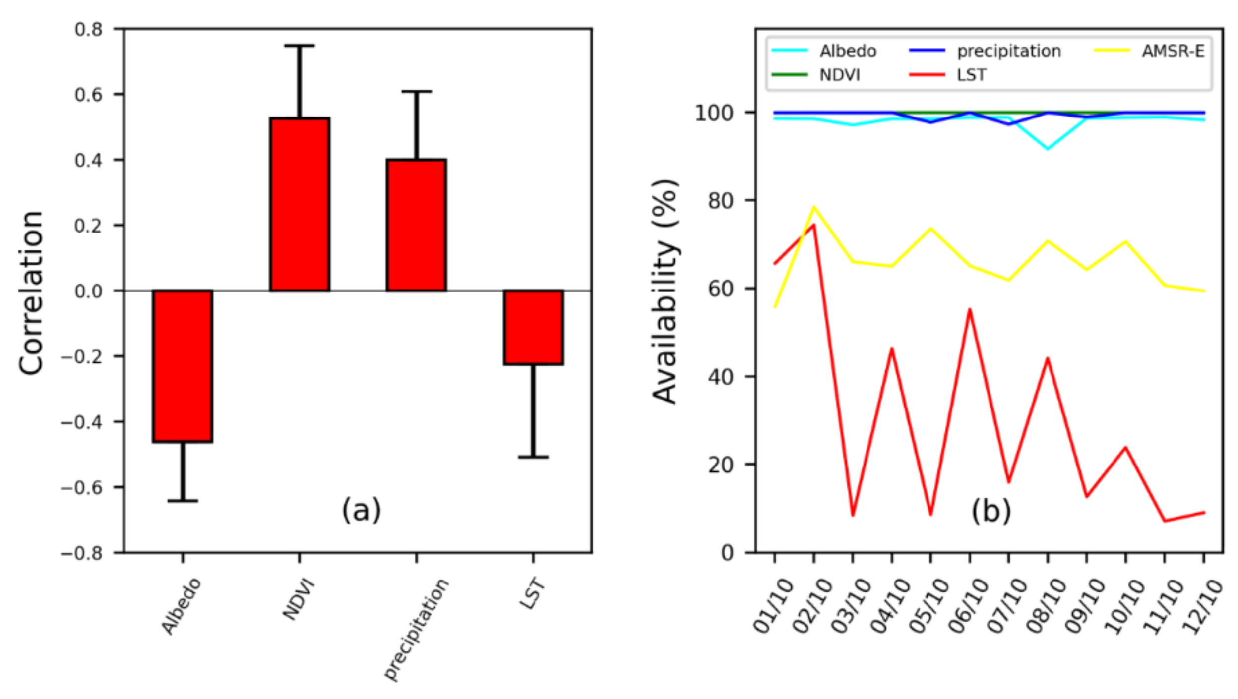
3.1. Correlation Analysis between Soil Moisture and Variables

As mentioned earlier, Albedo, NDVI, LST, and precipitation data were used as input variables in the RF-based SM relationship model. According to previous downscaling studies [39,54], these variables are closely related to SM.

This study analyzed the correlation between the used variables and SM according to the linear regression relationship, as shown in Figure 3a. In the whole study area, the correlation between SM and available variables is relatively high. Among them, the correlation between NDVI and SM is the highest, about 0.53. This is because NDVI can describe vegetation growth [55] and soil background conditions. The correlation between precipitation and SM is also high, about 0.40, relating to the fact that precipitation is the most obvious way for the atmosphere to affect SM [41]. Albedo and LST are also highly related to SM, which are −0.46 and −0.23, respectively. Albedo and LST are important variables in monitoring and SM downscaling due to their controlling role in surface energy exchange [56]. Overall, the results show the practicability of using these parameters in soil moisture downscaling.

The data was collected in 2009. When observing AMSR-E data, we found that the integrity of the data on the 10th was relatively high. Therefore, we selected the 10th of each month in 2009. Notice that the dataset used in this study is not very complete. The integrity of each scene data is counted here, as shown in Figure 3b. It can be observed that the integrity of precipitation, NDVI, and Albedo is relatively high; part of AMSR-E is missing; and LST data is the most missing. The correlation between LST and AMSR-E is not particularly high, which may also be related to its high degree of deletion.

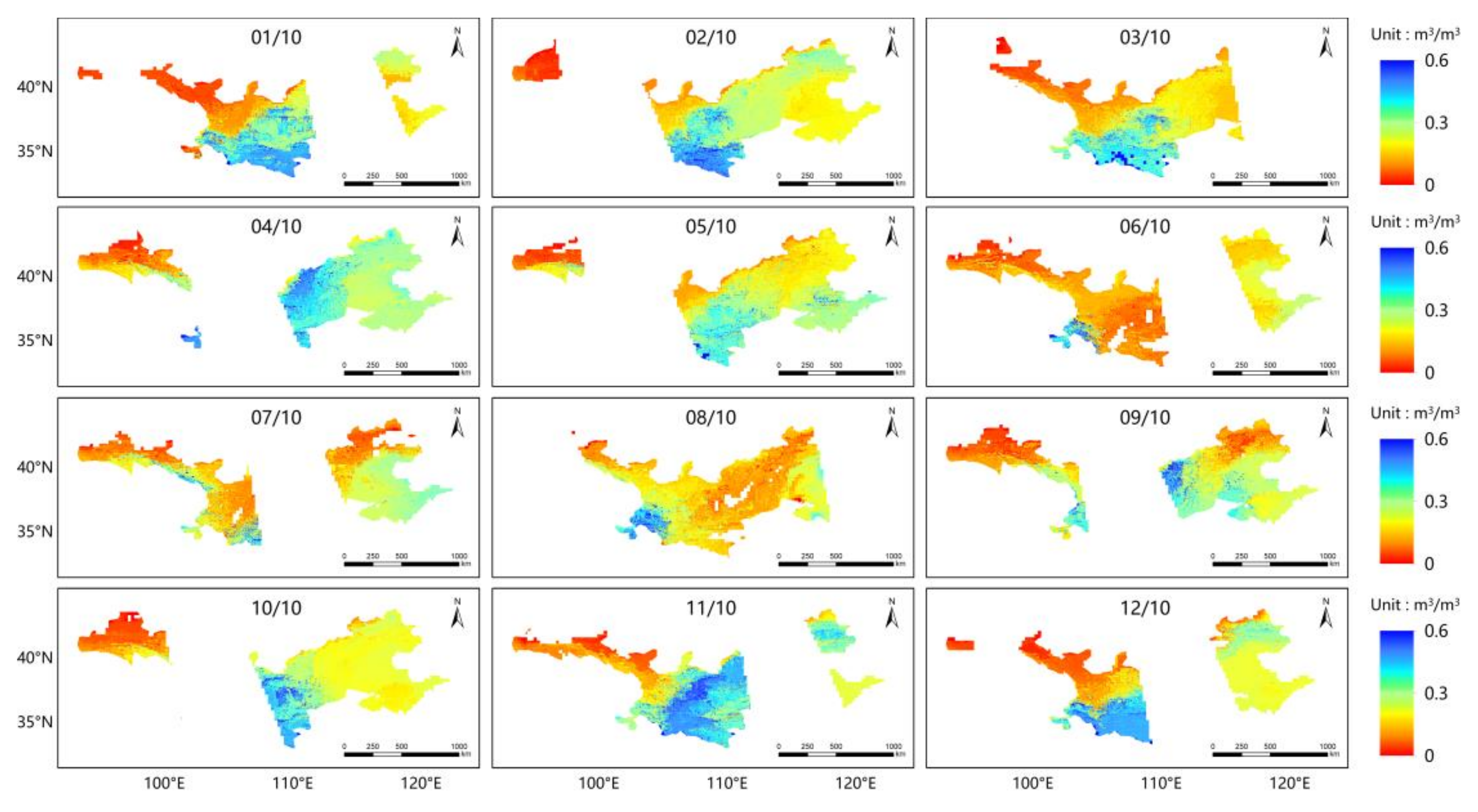
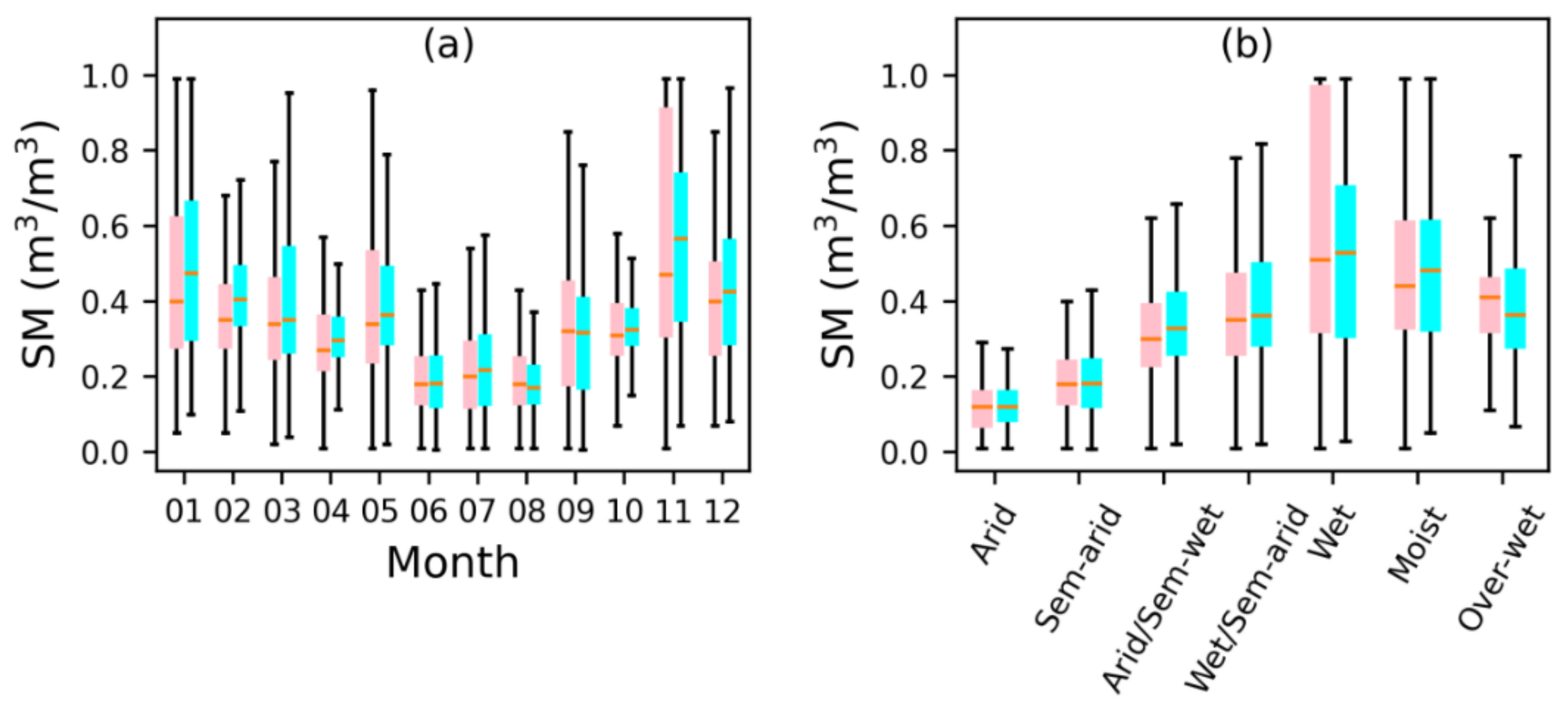
3.2. Spatial Distribution of Soil Moisture

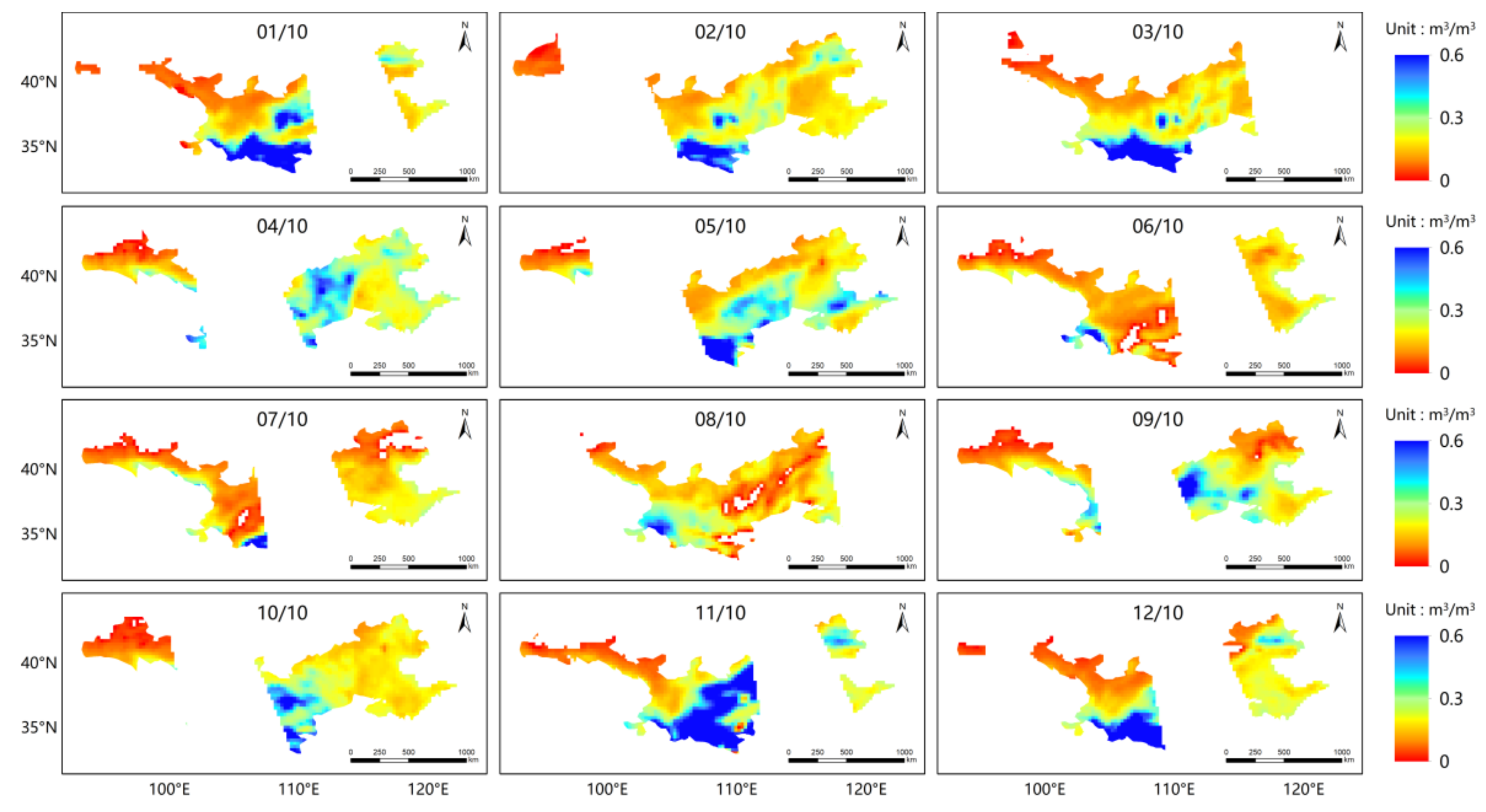
3.2.1. Spatial Distribution of AMSR-E and Downscaled Soil Moisture

Figure 4 and Figure 5 show the spatial distribution of AMSR-E soil moisture and the downscaled soil moisture, respectively. It can be found that, spatially, the soil moisture in the south is higher and that in the north is lower. In terms of time, the soil moisture is higher in November, December, and January, and lower in June, July, and August. Because of strong evapotranspiration in summer, the soil moisture is lower in summer and higher in winter. The downscaled results retain similar spatial patterns in the AMSR-E observations in most areas. At the same time, the spatial details of AMSR-E observations are also improved. The spatial distribution characteristics of the soil moisture after downscaling are generally consistent with the AMSR-E.

Comparing the images before and after downscaling, it can be seen visually that the downscaled image is much clearer and more detailed than the AMSR-E image. Overall, the performance of the downscaled data is relatively good, but it is overestimated or underestimated in some places. Specifically, the downscaled image is underestimated in the south with high soil moisture and overestimated in the north with low soil moisture. This is because machine learning methods tend to reduce the range of soil moisture data. In general, the visual consistency between the RF downscaled SM and the original AMSR-E SM is great.

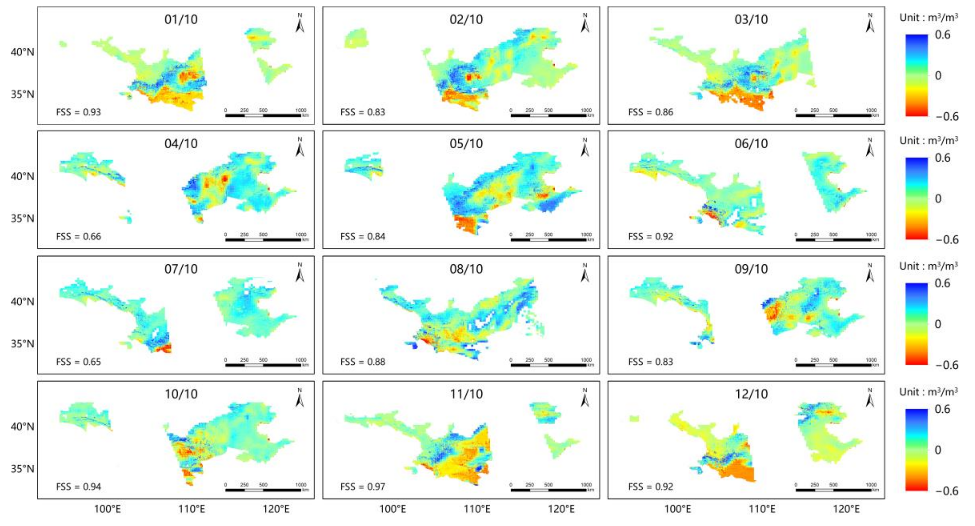
3.2.2. Difference between Downscaled Data and Soil Moisture of AMSR-E

To analyze the difference between AMSR-E and downscaled data, the box charts of 2 kinds of data in 12 months and the box charts classified by soil dry humidity were checked. Figure 6a shows the box diagram of AMSR-E and RF downscaled data for 12 months. It is observed that the differences between the 2 datasets are small in most months, and the values of the 2 data are basically kept within 0.1–0.6. Soil moisture is lower in June, July, and August, and higher in November, December, and January. As mentioned earlier, due to strong evapotranspiration in summer, soil moisture is lower in summer and higher in winter. At the same time, the RF results are generally high and overestimated. Earlier studies have shown similar results [57,58], probably relating to the fact that some high-resolution auxiliary data are added to better capture surface information and describe detailed information after higher resolution.

Figure 6b compares the two datasets after classified statistics according to dry humidity classification. In the seven dry moisture soil types, there is little difference between the two data. Meanwhile, it can be found that the RF results are generally high and overestimated; however, underestimation occurs in the over-wet region.

To further analyze the difference before and after downscaling, we subtracted the AMSR-E data from downscaled data to obtain the difference diagram. Figure 7 shows the difference between downscaled data and AMSR-E data, with FSS values at the bottom left of the graph. It is observed that the differences in most regions are relatively small. The places with underestimated phenomena are generally located in the south area with higher soil moisture. The overestimated phenomenon is located in the central and northern areas. This is consistent with earlier studies [1,46,59], which illustrate that machine learning methods tend to reduce the range of the target data. Therefore, the method will reduce the value of the high soil moisture area in the original AMSR-E data and increase the value of the low soil moisture area. The FSS values for all months are greater than 0.5, which shows good consistency of the data before and after downscaling. In general, the differences between the RF downscaled data and the original AMSR-E data are small, implying that the RF downscaled data and AMSR-E data have similar spatial patterns.

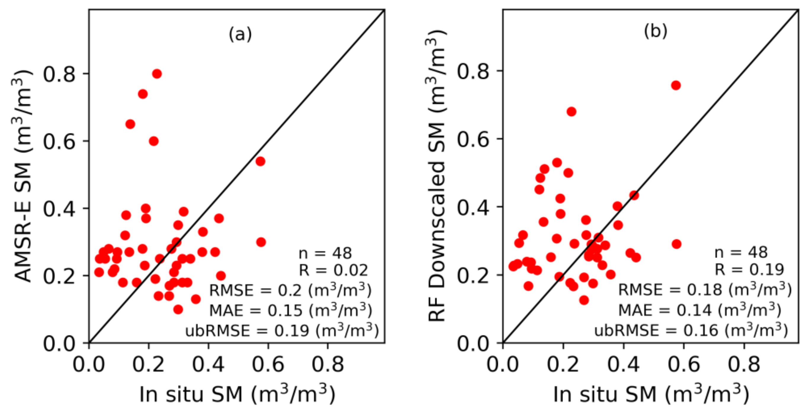
3.3. Evaluation with In Situ Measurements

In order to prove the effect of RF downscaling, we verified AMSR-E and the RF downscaled data with ground station data, respectively. Figure 8 shows the verification results of the AMSR-E and RF downscaled data with ground station data. It is observed that the performance of R, RMSE, MAE, and ubRMSE after downscaling is better than those of the AMSR-E. Among them, the R of the RF downscaled data is higher. The R of AMSR-E is 0.02, and the R of the RF downscaled result is 0.19. The RMSE, MAE, and ubRMSE of downscaled data are lower. The RMSE, MAE, and ubRMSE of AMSR-E are 0.20, 0.15, and 0.19 m³/m³, respectively. The RMSE, MAE, and ubRMSE of the RF downscaled results are 0.18, 0.14, and 0.16 m³/m³, respectively. Therefore, compared with AMSR-E data, the verification results of the RF downscaled data with in situ measurements are better and closer to the ground soil moisture. The large differences mainly occur in areas where the in situ soil moisture is large. This may be due to the lesser capacity to capture the evapotranspiration information well, thereby overestimating soil moisture. In general, it shows that the RF downscaling algorithm is reasonable and effective.

4. Discussion

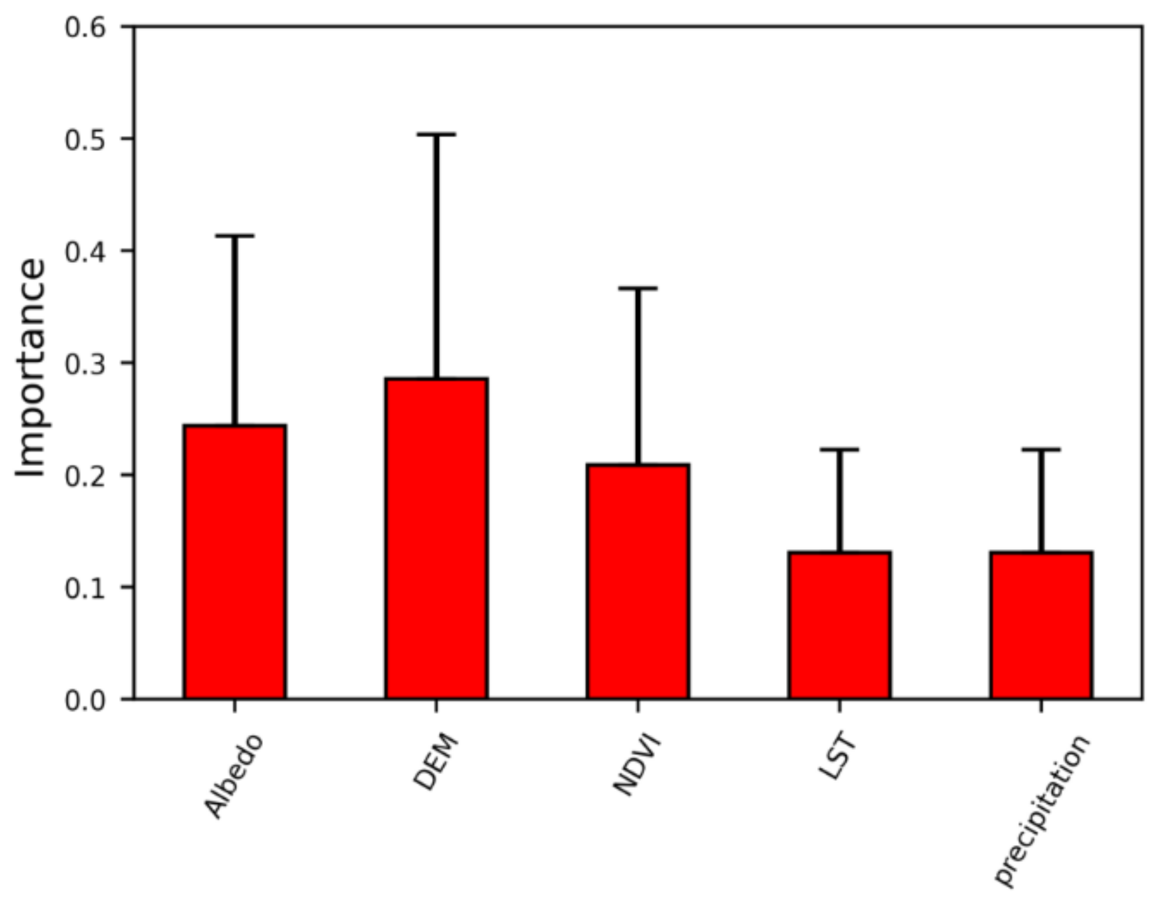
4.1. Importance Analysis of Explanatory Factors

Analyzing the importance of the five input explanatory factors (Albedo, DEM, NDVI, LST, and precipitation) to the downscaled SM results is critical to understand the impact of participating variables on the performance of the proposed RF method. The importance of these variables is described by the mean and standard deviation. We used the importance score, a key index provided by the RF algorithm [57], to analyze the contribution of each variable in the proposed method.

As shown in Figure 9, DEM is identified as the most important variable with an importance value of 0.29, because it can capture the spatial patterns and variations of the downscaled SM [1]. Albedo and NDVI have significant effects on RF modeling, and the importance values are 0.24 and 0.21, respectively, since they can reflect the surface energy flux and vegetation state [60]. The LST has importance with a value of 0.13 relating to the control effect of SM on land surface energy exchange [56]. Precipitation has the same results as LST, because precipitation is a vital parameter directly leading to variations in SM [46]. In general, the results show that it is reasonable to use these auxiliary data for soil moisture downscaling, demonstrating the certain impact of explanatory factors on RF modeling.

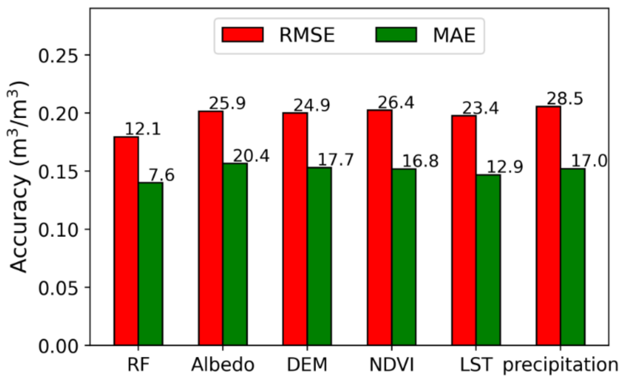
4.2. Leave-One-Out Analysis

Leave-one-out analysis was further conducted to verify the rationality and superiority of our model. Specifically, with this approach, the downscaling model was implemented after removing one input variable. Then, the downscaled results were verified with in situ observations. Figure 10 shows the verification results diagram of the leave-one-out approach. The first is the verification results of all parameters participating in random forest downscaling, followed by the verification results of the downscaled results with in situ data after removing these variables (Albedo, DEM, NDVI, LST, and precipitation, respectively). The numbers on the histogram are processed to better show their differences. The results of the random forest with all parameters involved are the best, and RMSE and MAE of RF are the lowest. Without precipitation and NDVI data, RMSE and MAE are increased significantly. Therefore, precipitation and NDVI have the greatest impact on the model results, followed by the Albedo, DEM, and LST data. Compared with the RF results, the RMSE and MAE of no-precipitation increased by 0.026 and 0.012 m³/m³, respectively. No-LST had the least impact on the results, and its RMSE and MAE increased by 0.018 and 0.007 m³/m³, respectively. Therefore, the addition of these five parameters can improve the performance of our proposed method and obtain better downscaling results.

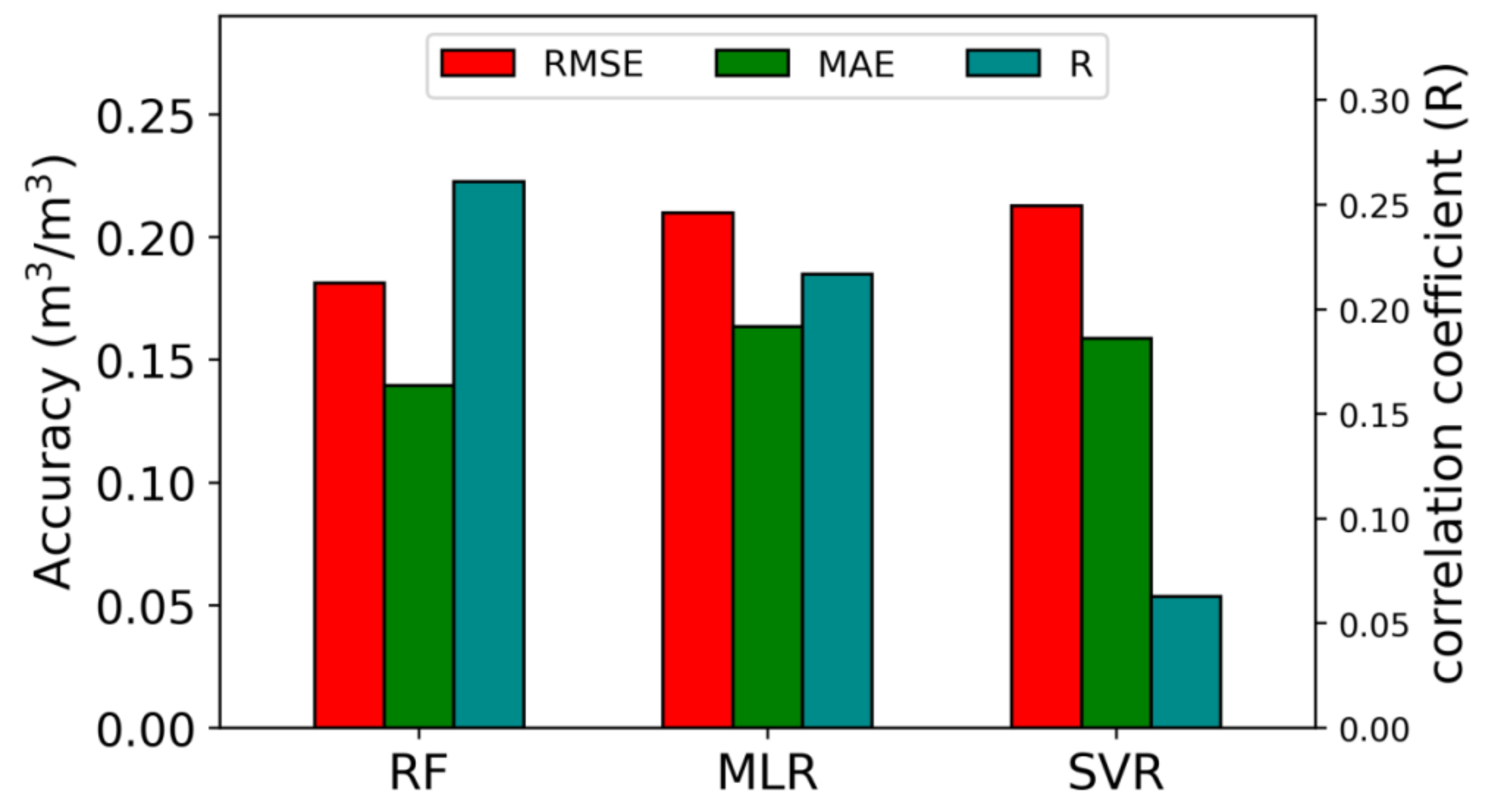
4.3. Comparison of Different Methods

To further verify the accuracy of the proposed downscaling approach, our study selected several methods that are often used in downscaling research to compare with the proposed RF method. Here, we compare the proposed RF method with Multiple Linear Regression (MLR) [61] and Support Vector Regression (SVR) [62]. The verification results of the downscaled data of these three methods with in situ observations were obtained. It is found from Figure 11 that the proposed RF method has the best results and significantly outperforms the other two methods. The RMSE and MAE of RF are lower than those of the other two methods, with an RMSE and MAE of 0.181 and 0.134 m³/m³, respectively. The R of RF is higher with a value of 0.261. At the same time, the performance of MLR is better than SVR, with lower RMSE and higher R.

The reason for the above results may be that the MLR model is suitable for simple linear regression. The MLR is prone to over-fitting [63] and is not suitable for large-scale research. The kernel function of the SVR model plays a vital role in the modeling process [64], but the type of kernel function and other parameters need to be selected artificially in the operation of the model. Hence, this problem may affect the final accuracy and prediction ability of the model and makes the accuracy poor. The RF model has randomness, which makes the model more stable and more generalized in the process of learning and application. The randomness of RF also reduces the occurrence of over-fitting to a great extent. Moreover, there are fewer artificially determined parameters in the operation process of the model, which avoids the interference of human factors.

The proposed method is compared with methods from several earlier studies. Four commonly used machine learning approaches [47] are first used for comparison. The polynomial fitting method [55], which is a popularly used method, is added for the comparative analysis. In addition, the UCLA downscaling method that was proposed by Kim and Hogue [65] is also used in the comparison. The study area, data used, and the corresponding accuracy of each method are shown in

Table 3. Comparison of different methods for downscaled SM against in situ soil moisture measurements (CART is classification and regression trees, KNN is K-nearest neighbors, BAYE is Bayesian regression, and RF is random forest).

Methods	Study Area	Data Used	R/R2	RMSE (m3/m3)	Reference Studies
CART	Heilongjiang, Jilin, and Liaoning Provinces, China	ESA CCI, MODIS	0.135	0.076	[47]
KNN			0.13	0.074
BAYE			0.081	0.075
RF			0.191	0.073
UCLA method	Southern Arizona, USA	AMSR-E, MODIS	0.27	0.051	[65]
Polynomial fitting method	AACES field, Australia	SMOS, MODIS	0.14–0.21	0.09–0.17	[55]
Proposes method	North China	AMSR-E, MODIS	0.19–0.26	0.18	-

. This study confirms that the proposed approach can be compared with other methods, or even better. The proposed method selected five kinds of effective auxiliary data and used an adaptive spatiotemporal window determination strategy. Compared with other methods, it is more suitable for application to complex large areas.

4.4. Limitations of the Study

This study successfully downscaled the AMSR-E data with 25 km resolution to 1 km; however, there are still some shortcomings. First, the study area focused on North China, where there are not many ground stations and verification data. Therefore, the verification results obtained have certain limitations. In future work, more field data can be collected for verification. Second, AMSR-E was selected for the original soil moisture data in this study. The quality of the original data may also affect the results of downscaling. We can use other high-quality data in the future. This study used some common statistical metrics to validate the results. More validation metrics, such as Empirical Orthogonal Functions (EOF) and SPAtial EFficiency metric (SAPAEF) [53,66,67], can be used in future work. In this study, downscaling soil moisture data were rarely applied. Future work can apply downscaling soil moisture data more widely [68,69,70] and combine it with other directions [71,72]. Finally, the proposed method in this study is mainly based on the random forest. Considering that the use of one method may cause errors, multiple methods can be assembled for downscaling in the future.

5. Conclusions

This study proposed an efficient framework based on the RF model to downscale AMSR-E soil moisture over North China from its original resolution of 25 km to a better resolution of 1 km. This study used an adaptive spatiotemporal window determination strategy and five auxiliary data (LST, NDVI, Albedo, precipitation, and DEM). The participating variables are closely related to soil moisture and were acquired from a satellite remote sensing dataset and ground-based observations. The downscaled image was better able to describe the details of soil moisture, and showed a consistent spatial pattern with the original AMSR-E SM. The main conclusions are given as follows.

(1) The overall R, RMSE, MAE, and ubRMSE between the downscaled SM produced by the proposed model and in situ measurements are 0.19, 0.18, 0.14, and 0.16 m³/m³, respectively. These results are better than those of the original AMSR-E SM, with R of 0.02, RMSE of 0.20 m³/m³, MAE of 0.15 m³/m³, and ubRMSE of 0.19 m³/m³, respectively. This means that the proposed downscaling algorithm is reasonable and effective.

(2) DEM, Albedo, precipitation, and LST show high importance for SM downscaling, indicating their efficiency as key variables closely related to SM changes. These results also show that the inclusion of all input variables leads to the best downscaling accuracy. At the same time, these variables combined with machine learning and spatiotemporal search algorithms can be applied to complex large areas.

(3) The proposed RF method significantly outperforms the MLR and SVR. The downscaled data acquired from the proposed downscaling method were also compared with MLR and SVR. The verification results with in situ measurements showed that the proposed approach is better than the other two methods. The R, RMSE, and MAE between the RF downscaled SM and in situ measurements are 0.261, 0.181, and 0.134 m³/m³, respectively. They are better than the results of the MLR and SVR. The R, RMSE, and MAE of the MLR downscaled SM are 0.217, 0.201, and 0.164 m³/m³, respectively. The R, RMSE, and MAE of the SVR downscaled SM are 0.063, 0.213, and 0.159 m³/m³, respectively.

In summary, this study successfully generated 1 km × 1 km SM data over North China, meeting the need for drought monitoring, hydrological modeling, and some related research. The merit of the proposed method is that there is no limit to land surface conditions, such as semiarid or humid areas. In the meantime, this method can be applied to large areas with various climate and surface characteristics. Future work will focus on collecting other SM data and more in situ observations, and using ensemble machine learning algorithms.

References

1. Abbaszadeh, P.; Moradkhani, H.; Zhan, X. Downscaling SMAP Radiometer Soil Moisture Over the CONUS Using an Ensemble Learning Method. Water Resour. Res. 2019, 55, 324–344. [Google Scholar] [CrossRef] [Green Version]
2. Zhang, T.; Peng, J.; Liang, W.; Yang, Y.T.; Liu, Y.X. Spatial-temporal patterns of water use efficiency and climate controls in China’s Loess Plateau during 2000–2010. Sci. Total Environ. 2016, 565, 105–122. [Google Scholar] [CrossRef] [PubMed]
3. Bindlish, R.; Crow, W.; Jackson, T.J. Role of Passive Microwave Remote Sensing in Improving Flood Forecasts. IEEE Geosci. Remote Sens. Lett. 2009, 6, 112–116. [Google Scholar] [CrossRef]
4. Mao, K.; Shi, J.; Tang, H.; Li, Z.-L.; Wang, X.; Chen, K.-S. A Neural Network Technique for Separating Land Surface Emissivity and Temperature From ASTER Imagery. IEEE Trans. Geosci. Remote Sens. 2007, 46, 200–208. [Google Scholar] [CrossRef]
5. Renzullo, L.J.; van Dijk, A.I.J.M.; Perraud, J.M.; Collins, D.; Henderson, B.; Jin, H.; Smith, A.B.; McJannet, D.L. Continental satellite soil moisture data assimilation improves root-zone moisture analysis for water resources assessment. J. Hydrol. 2014, 519, 2747–2762. [Google Scholar] [CrossRef]
6. Chen, C.F.; Son, N.T.; Chang, L.Y.; Chen, C.C. Monitoring of soil moisture variability in relation to rice cropping systems in the Vietnamese Mekong Delta using MODIS data. Appl. Geogr. 2011, 31, 463–475. [Google Scholar] [CrossRef]
7. Tuttle, S.; Salvucci, G. Empirical evidence of contrasting soil moisture-precipitation feedbacks across the United States. Science 2016, 352, 825–828. [Google Scholar] [CrossRef] [Green Version]
8. Liu, Y.Y.; Dorigo, W.A.; Parinussa, R.M.; de Jeu, R.A.; Wagner, W.; McCabe, M.F.; Evans, J.P.; Van Dijk, A.I.J.M. Trend-preserving blending of passive and active microwave soil moisture retrievals. Remote Sens. Environ. 2012, 123, 280–297. [Google Scholar] [CrossRef]
9. Krishnan, P.; Black, T.A.; Grant, N.J.; Barr, A.G.; Hogg, E.T.H.; Jassal, R.S.; Morgenstern, K. Impact of changing soil moisture distribution on net ecosystem productivity of a boreal aspen forest during and following drought. Agric. For. Meteorol. 2006, 139, 208–223. [Google Scholar] [CrossRef]
10. Dorigo, W.; Wagner, W.; Albergel, C.; Albrecht, F.; Balsamo, G.; Brocca, L.; Chung, D.; Ertl, M.; Forkel, M.; Gruber, A.; et al. ESA CCI Soil Moisture for improved Earth system understanding: State-of-the art and future directions. Remote Sens. Environ. 2017, 203, 185–215. [Google Scholar] [CrossRef]
11. Zhao, S.H.; Cong, D.M.; He, K.X.; Yang, H.; Qin, Z.H. Spatial-Temporal Variation of Drought in China from 1982 to 2010 Based on a modified Temperature Vegetation Drought Index (mTVDI). Sci. Rep. 2017, 7, 17173. [Google Scholar] [CrossRef]
12. Petropoulos, G.P.; Ireland, G.; Barrett, B. Surface soil moisture retrievals from remote sensing: Current status, products & future trends. Phys. Chem. Earth 2015, 83–84, 36–56. [Google Scholar] [CrossRef]
13. Peng, J.; Loew, A. Recent Advances in Soil Moisture Estimation from Remote Sensing. Water 2017, 9, 530. [Google Scholar] [CrossRef] [Green Version]
14. Engman, E.T.; Chauhan, N. Status of Microwave Soil-Moisture Measurements with Remote-Sensing. Remote Sens. Environ. 1995, 51, 189–198. [Google Scholar] [CrossRef]
15. Njoku, E.; Jackson, T.; Lakshmi, V.; Chan, T.; Nghiem, S. Soil moisture retrieval from AMSR-E. IEEE Trans. Geosci. Remote Sens. 2003, 41, 215–229. [Google Scholar] [CrossRef]
16. Entekhabi, D.; Njoku, E.G.; O’Neill, P.E.; Kellogg, K.H.; Crow, W.T.; Edelstein, W.N.; Entin, J.K.; Goodman, S.D.; Jackson, T.J.; Johnson, J.; et al. The Soil Moisture Active Passive (SMAP) Mission. Proc. IEEE 2010, 98, 704–716. [Google Scholar] [CrossRef]
17. Berger, M.; Camps, A.; Font, J.; Kerr, Y.; Miller, J.; Johannessen, J.A.; Boutin, J.; Drinkwater, M.R.; Skou, N.; Floury, N.; et al. Measuring ocean salinity with ESA’s SMOS mission-Advancing the science. ESA Bull. 2002, 111, 113–121. [Google Scholar]
18. Molero, B.; Merlin, O.; Malbeteau, Y.; Al Bitar, A.; Cabot, F.; Stefan, V.; Kerr, Y.; Bacon, S.; Cosh, M.H.; Bindlish, R.; et al. SMOS disaggregated soil moisture product at 1 km resolution: Processor overview and first validation results. Remote Sens. Environ. 2016, 180, 361–376. [Google Scholar] [CrossRef]
19. Njoku, E.G.; Entekhabi, D. Passive microwave remote sensing of soil moisture. J. Hydrol. 1996, 184, 101–129. [Google Scholar] [CrossRef]
20. Schmugge, T. Applications of passive microwave observations of surface soil moisture. J. Hydrol. 1998, 212, 188–197. [Google Scholar] [CrossRef]
21. Jin, Y.; Ge, Y.; Liu, Y.J.; Chen, Y.H.; Zhang, H.T.; Heuvelink, G.B.M. A Machine Learning-Based Geostatistical Downscaling Method for Coarse-Resolution Soil Moisture Products. IEEE J. Sel. Top. Appl. Earth Obs. Remote Sens. 2021, 14, 1025–1037. [Google Scholar] [CrossRef]
22. Peng, J.; Loew, A.; Merlin, O.; Verhoest, N.E.C. A review of spatial downscaling of satellite remotely sensed soil moisture. Rev. Geophys. 2017, 55, 341–366. [Google Scholar] [CrossRef]
23. de Jeu, R.A.M.; Wagner, W.; Holmes, T.R.H.; Dolman, A.J.; van de Giesen, N.C.; Friesen, J. Global Soil Moisture Patterns Observed by Space Borne Microwave Radiometers and Scatterometers. Surv. Geophys. 2008, 29, 399–420. [Google Scholar] [CrossRef] [Green Version]
24. Merlin, O.; Walker, J.P.; Chehbouni, A.; Kerr, Y. Towards deterministic downscaling of SMOS soil moisture using MODIS derived soil evaporative efficiency. Remote Sens. Environ. 2008, 112, 3935–3946. [Google Scholar] [CrossRef] [Green Version]
25. Busch, F.A.; Niemann, J.D.; Coleman, M. Evaluation of an empirical orthogonal function-based method to downscale soil moisture patterns based on topographical attributes. Hydrol. Process. 2012, 26, 2696–2709. [Google Scholar] [CrossRef]
26. Peng, J.; Borsche, M.; Liu, Y.; Loew, A. How representative are instantaneous evaporative fraction measurements of daytime fluxes? Hydrol. Earth Syst. Sci. 2013, 17, 3913–3919. [Google Scholar] [CrossRef]
27. Ines, A.V.M.; Mohanty, B.P.; Shin, Y. An unmixing algorithm for remotely sensed soil moisture. Water Resour. Res. 2013, 49, 408–425. [Google Scholar] [CrossRef]
28. Loew, A.; Mauser, W. On the disaggregation of passive microwave soil moisture data using a priori knowledge of temporally persistent soil moisture fields. IEEE Trans. Geosci. Remote Sens. 2008, 46, 819–834. [Google Scholar] [CrossRef]
29. Lievens, H.; Tomer, S.K.; Al Bitar, A.; De Lannoy, G.J.M.; Drusch, M.; Dumedah, G.; Franssen, H.J.H.; Kerr, Y.H.; Martens, B.; Pan, M.; et al. SMOS soil moisture assimilation for improved hydrologic simulation in the Murray Darling Basin, Australia. Remote Sens. Environ. 2015, 168, 146–162. [Google Scholar] [CrossRef]
30. Njoku, E.G.; Wilson, W.J.; Yueh, S.H.; Dinardo, S.J.; Li, F.K.; Jackson, T.J.; Lakshmi, V.; Bolten, J. Observations of soil moisture using a passive and active low-frequency microwave airborne sensor during SGP99. IEEE Trans. Geosci. Remote Sens. 2002, 40, 2659–2673. [Google Scholar] [CrossRef]
31. Merlin, O.; Rudiger, C.; Al Bitar, A.; Richaume, P.; Walker, J.P.; Kerr, Y.H. Disaggregation of SMOS Soil Moisture in Southeastern Australia. IEEE Trans. Geosci. Remote Sens. 2012, 50, 1556–1571. [Google Scholar] [CrossRef] [Green Version]
32. Werbylo, K.L.; Niemann, J.D. Evaluation of sampling techniques to characterize topographically-dependent variability for soil moisture downscaling. J. Hydrol. 2014, 516, 304–316. [Google Scholar] [CrossRef] [Green Version]
33. Ranney, K.J.; Niemann, J.D.; Lehman, B.M.; Green, T.R.; Jones, A.S. A method to downscale soil moisture to fine resolutions using topographic, vegetation, and soil data. Adv. Water Resour. 2015, 76, 81–96. [Google Scholar] [CrossRef] [Green Version]
34. Pelletier, C.; Valero, S.; Inglada, J.; Champion, N.; Dedieu, G. Assessing the robustness of Random Forests to map land cover with high resolution satellite image time series over large areas. Remote Sens. Environ. 2016, 187, 156–168. [Google Scholar] [CrossRef]
35. Park, S.; Park, S.; Im, J.; Rhee, J.; Shin, J.; Park, J.D. Downscaling GLDAS Soil Moisture Data in East Asia through Fusion of Multi-Sensors by Optimizing Modified Regression Trees. Water 2017, 9, 332. [Google Scholar] [CrossRef] [Green Version]
36. Imaoka, K.; Kachi, M.; Fujii, H.; Murakami, H.; Hori, M.; Ono, A.; Igarashi, T.; Nakagawa, K.; Oki, T.; Honda, Y.; et al. Global Change Observation Mission (GCOM) for Monitoring Carbon, Water Cycles, and Climate Change. Proc. IEEE 2010, 98, 717–734. [Google Scholar] [CrossRef]
37. Merlin, O.; Malbeteau, Y.; Notfi, Y.; Bacon, S.; Er-Raki, S.; Khabba, S.; Jarlan, L. Performance Metrics for Soil Moisture Downscaling Methods: Application to DISPATCH Data in Central Morocco. Remote Sens. 2015, 7, 3783–3807. [Google Scholar] [CrossRef] [Green Version]
38. Fang, B.; Lakshmi, V. Soil moisture at watershed scale: Remote sensing techniques. J. Hydrol. 2014, 516, 258–272. [Google Scholar] [CrossRef]
39. Wilson, D.J.; Western, A.W.; Grayson, R.B. A terrain and data-based method for generating the spatial distribution of soil moisture. Adv. Water Resour. 2005, 28, 43–54. [Google Scholar] [CrossRef]
40. Mascaro, G.; Vivoni, E.R.; Deidda, R. Soil moisture downscaling across climate regions and its emergent properties. J. Geophys. Res. Earth Surf. 2011, 116, D22114. [Google Scholar] [CrossRef] [Green Version]
41. Crow, W.T.; Berg, A.A.; Cosh, M.H.; Loew, A.; Mohanty, B.P.; Panciera, R.; de Rosnay, P.; Ryu, D.; Walker, J.P. Upscaling Sparse Ground-Based Soil Moisture Observations for the Validation of Coarse-Resolution Satellite Soil Moisture Products. Rev. Geophys. 2012, 50, RG2002. [Google Scholar] [CrossRef] [Green Version]
42. Jones, A.R.; Brunsell, N.A. A scaling analysis of soil moisture-precipitation interactions in a regional climate model. Theor. Appl. Climatol. 2009, 98, 221–235. [Google Scholar] [CrossRef]
43. Yang, K.; He, J.; Tang, W.J.; Qin, J.; Cheng, C.C.K. On downward shortwave and longwave radiations over high altitude regions: Observation and modeling in the Tibetan Plateau. Agric. For. Meteorol. 2010, 150, 38–46. [Google Scholar] [CrossRef]
44. He, J.; Yang, K.; Tang, W.J.; Lu, H.; Qin, J.; Chen, Y.Y.; Li, X. The first high-resolution meteorological forcing dataset for land process studies over China. Sci. Data 2020, 7, 25. [Google Scholar] [CrossRef] [Green Version]
45. Breiman, L. Random forests. Mach. Learn 2001, 45, 5–32. [Google Scholar] [CrossRef] [Green Version]
46. Long, D.; Bai, L.; Yan, L.; Zhang, C.; Yang, W.; Lei, H.; Quan, J.; Meng, X.; Shi, C. Generation of spatially complete and daily continuous surface soil moisture of high spatial resolution. Remote Sens. Environ. 2019, 233, 111364. [Google Scholar] [CrossRef]
47. Liu, Y.X.Y.; Yang, Y.P.; Jing, W.L.; Yue, X.F. Comparison of Different Machine Learning Approaches for Monthly Satellite-Based Soil Moisture Downscaling over Northeast China. Remote Sens. 2018, 10, 31. [Google Scholar] [CrossRef] [Green Version]
48. Liu, K.; Su, H.; Li, X.; Chen, S. Development of a 250-m Downscaled Land Surface Temperature Data Set and Its Application to Improving Remotely Sensed Evapotranspiration Over Large Landscapes in Northern China. IEEE Trans. Geosci. Remote Sens. 2020, 10, 31. [Google Scholar] [CrossRef]
49. Udovicic, M.; Bazdaric, K.; Bilic-Zulle, L.; Petrovecki, M. What we need to know when calculating the coefficient of correlation? Biochem. Med. 2007, 17, 10–15. [Google Scholar] [CrossRef] [Green Version]
50. Tan, S.; Wu, B.F.; Yan, N.N.; Zhu, W.W. An NDVI-Based Statistical ET Downscaling Method. Water 2017, 9, 995. [Google Scholar] [CrossRef] [Green Version]
51. Zuo, J.P.; Xu, J.H.; Chen, Y.N.; Wang, C. Downscaling Precipitation in the Data-Scarce Inland River Basin of Northwest China Based on Earth System Data Products. Atmosphere 2019, 10, 613. [Google Scholar] [CrossRef] [Green Version]
52. Roberts, N.M.; Lean, H.W.J. Scale-selective verification of rainfall accumulations from high-resolution forecasts of convective events. Mon. Weather Rev. 2008, 136, 78–97. [Google Scholar] [CrossRef]
53. Skok, G.; Roberts, N.J. Analysis of fractions skill score properties for random precipitation fields and ECMWF forecasts. Q. J. R. Meteorol. Soc. 2016, 142, 2599–2610. [Google Scholar] [CrossRef]
54. Srivastava, P.K.; Han, D.W.; Ramirez, M.R.; Islam, T. Machine Learning Techniques for Downscaling SMOS Satellite Soil Moisture Using MODIS Land Surface Temperature for Hydrological Application. Water Resour. Manag. 2013, 27, 3127–3144. [Google Scholar] [CrossRef]
55. Piles, M.; Camps, A.; Vall-Llossera, M.; Corbella, I.; Panciera, R.; Rudiger, C.; Kerr, Y.H.; Walker, J. Downscaling SMOS-Derived Soil Moisture Using MODIS Visible/Infrared Data. IEEE Trans. Geosci. Remote Sens. 2011, 49, 3156–3166. [Google Scholar] [CrossRef]
56. Wang, J.R.; Choudhury, B.J. Remote-Sensing of Soil-Moisture Content over Bare Field at 1.4 Ghz Frequency. J. Geophys. Res. Oceans 1981, 86, 5277–5282. [Google Scholar] [CrossRef]
57. Im, J.; Park, S.; Rhee, J.; Baik, J.; Choi, M. Downscaling of AMSR-E soil moisture with MODIS products using machine learning approaches. Environ. Earth Sci. 2016, 75, 1120. [Google Scholar] [CrossRef]
58. Zhao, W.; Li, A.N. A Downscaling Method for Improving the Spatial Resolution of AMSR-E Derived Soil Moisture Product Based on MSG-SEVIRI Data. Remote Sens. 2013, 5, 6790–6811. [Google Scholar] [CrossRef] [Green Version]
59. Liu, Y.X.Y.; Xia, X.L.; Yao, L.; Jing, W.L.; Zhou, C.H.; Huang, W.M.; Li, Y.; Yang, J. Downscaling Satellite Retrieved Soil Moisture Using Regression Tree-Based Machine Learning Algorithms Over Southwest France. Earth Space Sci. 2020, 7, e2020EA001267. [Google Scholar] [CrossRef]
60. Park, S.; Im, J.; Park, S.; Rhee, J. Drought monitoring using high resolution soil moisture through multi-sensor satellite data fusion over the Korean peninsula. Agric. For. Meteorol. 2017, 237, 257–269. [Google Scholar] [CrossRef]
61. Wilks, D.S. Statistical Methods in the Atmospheric Sciences; Academic Press: Cambridge, MA, USA, 2011; Volume 100. [Google Scholar]
62. Tripathi, S.; Srinivas, V.; Nanjundiah, R.S. Downscaling of precipitation for climate change scenarios: A support vector machine approach. J. Hydrol. 2006, 330, 621–640. [Google Scholar] [CrossRef]
63. Xie, W.H.; Yi, S.Z.; Leng, C. A Study to Compare Three Different Spatial Downscaling Algorithms of Annual TRMM 3B43 Precipitation. In Proceedings of the 26th International Conference on Geoinformatics, Kunming, China, 28–30 June 2018. [Google Scholar] [CrossRef]
64. Ebrahimy, H.; Azadbakht, M. Downscaling MODIS land surface temperature over a heterogeneous area: An investigation of machine learning techniques, feature selection, and impacts of mixed pixels. Comput. Geosci. 2019, 124, 93–102. [Google Scholar] [CrossRef]
65. Kim, J.; Hogue, T.S. Improving Spatial Soil Moisture Representation Through Integration of AMSR-E and MODIS Products. IEEE Trans. Geosci. Remote Sens. 2012, 50, 446–460. [Google Scholar] [CrossRef]
66. Koch, J.; Demirel, M.C.; Stisen, S.J. The SPAtial EFficiency metric (SPAEF): Multiple-component evaluation of spatial patterns for optimization of hydrological models. Geosci. Model Dev. 2018, 11, 1873–1886. [Google Scholar] [CrossRef] [Green Version]
67. Ahmed, K.; Sachindra, D.A.; Shahid, S.; Demirel, M.C.; Chung, E.-S.J.H.; Sciences, E.S. Selection of multi-model ensemble of general circulation models for the simulation of precipitation and maximum and minimum temperature based on spatial assessment metrics. Hydrol. Earth Syst. Sci. 2019, 23, 4803–4824. [Google Scholar] [CrossRef] [Green Version]
68. Liu, K.; Wang, S.; Li, X.; Wu, T.J. Spatially disaggregating satellite land surface temperature with a nonlinear model across agricultural areas. J. Geophys. Res. Biogeosci. 2019, 124, 3232–3251. [Google Scholar] [CrossRef]
69. Liu, K.; Wang, S.; Li, X.; Li, Y.; Zhang, B.; Zhai, R. The assessment of different vegetation indices for spatial disaggregating of thermal imagery over the humid agricultural region. Int. J. Remote Sens. 2020, 41, 1907–1926. [Google Scholar] [CrossRef]
70. Liu, K.; Su, H.; Tian, J.; Li, X.; Wang, W.; Yang, L.; Liang, H. Assessing a scheme of spatial-temporal thermal remote-sensing sharpening for estimating regional evapotranspiration. Int. J. Remote Sens. 2018, 39, 3111–3137. [Google Scholar] [CrossRef]
71. Liu, K.; Su, H.; Li, X.; Chen, S.; Zhang, R.; Wang, W.; Yang, L.; Liang, H.; Yang, Y. A thermal disaggregation model based on trapezoid interpolation. IEEE J. Sel. Top. Appl. Earth Obs. Remote Sens. 2018, 11, 808–820. [Google Scholar] [CrossRef]
72. Liu, K.; Li, X.; Long, X. Trends in groundwater changes driven by precipitation and anthropogenic activities on the southeast side of the Hu Line. Environ. Res. Lett. 2021, 16, 094032. [Google Scholar] [CrossRef]
Figure 1. (a) Elevation and (b) dry humidity classification map of the study area. The black spots are the locations of the selected ground stations in this study.
Ijgi 11 00101 g001
Figure 3. (a) The correlation between soil moisture and each parameter factor is the correlation coefficient (R) calculated according to the linear regression between the used variables and AMSR-E. The red bar is the average value, and the black line is the standard deviation. (b) The integrity of each parameter.
Ijgi 11 00101 g003
Figure 4. Spatial distribution map of AMSR-E soil moisture on the 10th of each month.
Ijgi 11 00101 g004
Figure 5. Spatial distribution map of the RF downscaled soil moisture on the 10th of each month.
Ijgi 11 00101 g005
Figure 6. (a) Box chart of AMSR-E and the RF downscaled data for 12 months; (b) box diagram of AMSR-E and the RF downscaled data after classification by dry humidity (AMSR-E in red and downscaling data in blue).
Ijgi 11 00101 g006
Figure 7. Difference between downscaled data and AMSR-E data (FSS values are shown at the bottom left of the graph).
Ijgi 11 00101 g007
Figure 8. The verification results of (a) AMSR-E, (b) RF downscaled data with in situ measurements.
Ijgi 11 00101 g008
Figure 9. The importance of explanatory factors determined by the model. The red bar is the mean value and the black line is the standard deviation.
Ijgi 11 00101 g009
Figure 10. Verification results of the leave-one-out approach (the first is the verification results that all parameters participate in random forest downscaling, followed by the verification results after removing the corresponding parameters).
Ijgi 11 00101 g010
Figure 11. Comparison of three methods (RF is the proposed method, MLR is Multiple Linear Regression, and SVR is Support Vector Regression).
Ijgi 11 00101 g011