Improving LST Downscaling Quality on Regional and Field-Scale by Parameterizing the DisTrad Method

Abstract

Many scientists have been investigating Land Surface Temperature (LST) because of its relevance in water management science due to its direct influence on the hydrological water cycle. This effect stems from being one of the most significant variables influencing evapotranspiration. One of the most important reasons for the evapotranspiration retrieved from MODIS data’s limited suitability for scheduling and planning irrigation schemes is the lack of spatial resolution. As a result, high-resolution LST is required for estimating evapotranspiration. The goal of this study is to improve the resolution of the available LST data, to improve evapotranspiration (ET_a) estimation using statistical downscaling with Normalized Difference Vegetation Index (NDVI) as a predictor. The DisTrad (Disaggregation of Radiometric Surface Temperature) method was used for the LST downscaling procedure, which is based on aggregating the NDVI map to the LST map resolution and then calculating the coefficient of variation of the native NDVI map within the aggregated pixel and classifying the aggregated map into three classes: NDVI < 0.2 for the bare soil, 0.2 ≤ NDVI ≤ 0.5 for the partial vegetation, and NDVI > 0.5 for the full vegetation. DisTrad uses 25% of the pixels with the lowest coefficient of variation from each class to calculate the regression coefficients. In this work, adjustments to the DisTrad method were implemented to enhance downscaling LST and to examine the impacts of that alteration on the evapotranspiration estimation. The linear regression model was tested as an alternative to the original second-order polynomial. In using 10% of the pixels instead of the originally proposed 25% with the lowest coefficient of variation values, it is assumed that a group of pixels with a lower coefficient of variation represents a more homogeneous area, thus it gives more accurate values. The downscaled LST map retrieval was validated using Landsat 8 thermal maps (100 m). Applying the modified DisTrad approach to disaggregate Landsat LST to 30 m (NDVI resolution) yielded an R² of 0.72 for the 10%, 0.74 for the 25% and 0.61 for the second-order polynomial lowest coefficient of variation compared to native LST Landsat, which means that 10% can be used as an alternative. Applying the downscaled LST map to estimate ET_a yielded R² 0.84 in both cases, compared to ET_a yielded from the native Landsat LST. These results prove that using the robust linear regression provided better results than using polynomial regression. With the downscaled Land Surface Temperature data, it was possible to create detailed ET_a maps of the small agricultural fields in the test area.

1. Introduction

Evapotranspiration (ET) is a challenging parameter to estimate, but Land Surface Temperature (LST) and soil moisture are crucial parameters to assess it [1,2,3,4]. This effect is one of the most prominent factors affecting evapotranspiration [5,6,7,8]. Deriving Land Surface Temperature from thermal remote sensing is one of the most promising means of achieving the mission, whether at the regional or global scale [1,9,10]. The emergence of thermal sensors with high spatial resolution has improved and raised the quality of calculating LST [11,12], as these sensors have a spatial resolution of 60–100 m. However, with this high spatial resolution, poor temporal resolution due to 16 days revisit time for these sensors remains a challenge [13,14]. One of these sensors is the Landsat 8 OLI TIRS, which has two thermal bands with 100 m resolution and Landsat 7 thermal band with 60 m resolution [15,16]. On the other hand, several sensors with low spatial resolution produce high temporal resolution images with a repetition time varying from less than an hour to three days [2,13,17,18]. The poor spatial resolution of the evapotranspiration retrieved from MODIS data is one of the most important reasons for its limited suitability for scheduling and planning irrigation [18,19]. In developing countries, the agricultural lands are partitioned into small fields of less than 1 square kilometer.

Applying coarse-resolution thermal data to the small fields, one faces a problem called the thermal mixing effect, resulting from the differences in the thermal properties of the land cover classes within one pixel. Therefore, this problem needs to be addressed, e.g., by finding a relationship between the temporal and spatial resolutions of the thermal images [20].

The downscaling process is defined as increasing spatial resolution by finding values of the smaller pixels as a function of the original measurement with the coarse pixel size and some additional information, or, in a simplified way, and it can be described as decreasing the pixel size [21,22]. Many different approaches have been followed for the downscaling of LST [20], but the most popular approach is the disaggregation of LST based on a co-variable. The approach improves the resolution of LST, whether spatially or temporally, and makes it suitable for many applications, e.g., all applications that include the surface energy balance (SEB) [7,23]. One of the famous disaggregation methods is DisTrad (Disaggregation Procedure of Radiometric Surface Temperature [24]). Its principle is to find a mathematical relationship between the Radiometric Surface Temperature, and the Normalized Difference Vegetation Index NDVI through the inverse relationship between the LST and the NDVI [2,24,25,26,27]. A further developed approach is TsHARP (Temperature Sharpening), which is a modulation of the DisTrad, based on a linear relationship between the vegetation fractional cover (FC) and LST [28].

To parameterize the regression equation between the vegetation index and the Surface Temperature, Kustas et al. [24] have developed a process of aggregating the NDVI map and then calculating the coefficient of variation (CV) of the native NDVI values within each pixel in the aggregated map, using 25% of the aggregated pixels with the lowest coefficients of variation for defining the coefficients of the regression equation [24]. This approach was successfully tested on homogenous areas, but when used on heterogeneous areas, the problem of representativity occurs. Accordingly, the approach needs to be improved for heterogeneous regions [20,29]. This work aims to improve the DisTrad approach for downscaling LST for heterogeneous areas and improve the temporal and spatial distribution of the calculated high-resolution evapotranspiration maps.

The study’s specific goals are as follows: (a) Compare linear vs. polynomial based statistical downscaling, (b) compare 25% and 10% aggregated pixels with the lowest coefficients of variation, (c) improve ETa spatial and temporal resolution for the agricultural sector.

2. Materials and Methods

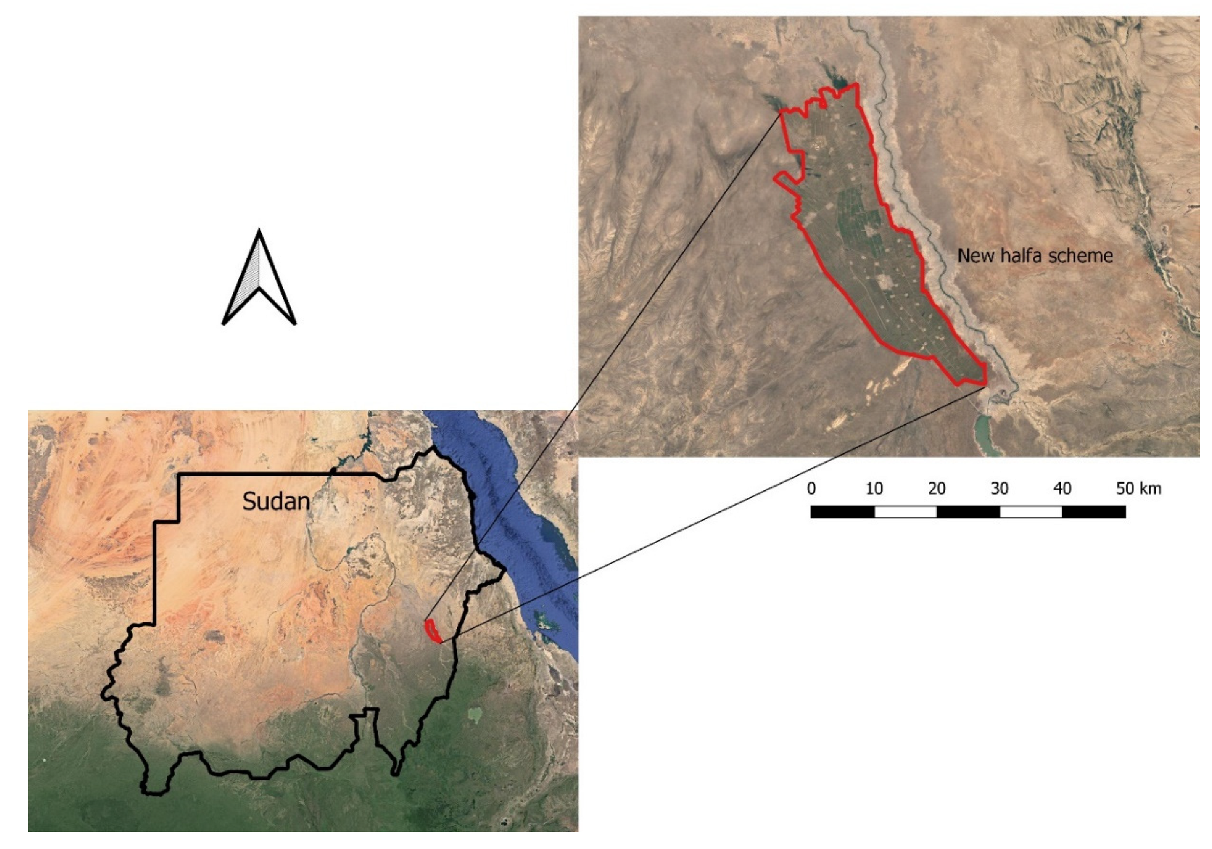
2.1. Study Area

The construction of the Aswan High Dam caused the inundation of the old town of Wadi Halfa by Lake Nasser. The New Halfa Agricultural Scheme was initiated in response as Sudan’s largest resettlement project. The New Halfa Agricultural Scheme is a 185,000-ha agricultural settlement scheme on the western side of Kassala State, roughly 400 km east of Khartoum [30]. The project is located on the Butana plain, along the Atbara River. At the time of its construction, the New Halfa Scheme was Sudan’s second-largest irrigation project after the Gezira Scheme, which is still the world’s largest irrigation scheme. Sudan’s irrigation agency manages the water through the Khasm el Girba dam on the Atbara River [31]. The irrigation system is gravity-fed, with the main canal transporting water to the project area via a network of subsidiary canals and motorized pumps in the small scheme areas. The irrigation system includes main canals, branch canals, minor canals, quaternary canals, and tertiary farm ditches. Field irrigation is done using the traditional basin (Angaya) approach, dividing the field into small sections. There are significant water losses in the system, reducing the available freshwater supplies, like evaporation, conveyance losses due to infiltration, etc. [31]. The dam was initially intended to store 1.3 billion cubic meters of water. However, by 1976, the reservoir’s storage capacity had been decreased to 0.8 billion cubic meters due to significant siltation originating from the upstream catchment of the river Atbara in Ethiopia’s highlands [30]. The reservoir’s capacity is now about 0.6 billion m³. During the growing season, the water in the smaller canals typically flows permanently. Farmers, however, have complained that some regions receive more water than others. Since the reservoir’s capacity is dwindling, the irrigated area is shrinking too. Each agricultural settler was given a 15-feddan hawasha (6.3 ha) (tenancy) to cultivate cotton, wheat, sorghum, and groundnuts. Mostly cotton was chosen since it is the most important cash crop for the government to provide hard currency and profit for the tenants. Groundnuts are the scheme’s second most significant cash crop, and wheat and sorghum were grown with any surplus sold [31]. Figure 1 shows the location map of the study area.

2.2. The DisTrad Downscaling Procedure for Radiometric Surface Temperature

For finding a mathematical relationship between the Radiometric Surface Temperature and the Normalized Difference Vegetation Index (NDVI) [24] suggested aggregating the fine-resolution NDVI map to the same coarse-resolution as the LST map and then defining the regression coefficients of Equation (1) with a least square fitting using a second-order polynomial.

$$\mathit{L}\mathit{S}{\mathit{T}}_{\mathit{C}\mathit{R}}^{\mathbf{*}}\mathbf{=}\mathit{a}\mathbf{+}\mathit{b} \mathit{N}\mathit{D}\mathit{V}{\mathit{I}}_{\mathit{C}\mathit{R}}\mathbf{+}\mathit{c} \mathit{N}\mathit{D}\mathit{V}{\mathit{I}}_{\mathit{C}\mathit{R}}^{\mathbf{2}}$$

(1)

where:

$\mathit{L}\mathit{S}{\mathit{T}}_{\mathit{C}\mathit{R}}^{\mathbf{*}}$: Land surface temperature at the coarser resolution (°C).

$\mathit{N}\mathit{D}\mathit{V}{\mathit{I}}_{\mathit{C}\mathit{R}}$: Aggregated normalized difference vegetation index at the coarser resolution.

The LST is influenced by the vegetation cover and other factors, such as soil moisture [32]. When these factors are overlooked during the downscaling process, the results are affected by the spatial variation of the factor values. To overcome this problem, Kustas et al. [24] used the difference between the aggregated downscaled LST and the original one (Equation (2)) for each pixel to estimate the error that represented the influence of other factors, such as soil moisture, and then used it for correction by Equation (3).

$$\mathbf{∆}{\widehat{\mathit{T}}}_{\mathit{C}\mathit{R}}\mathbf{=}\mathit{L}\mathit{S}{\mathit{T}}_{\mathit{C}\mathit{R}}\mathbf{-}{\widehat{\mathit{L}\mathit{S}\mathit{T}}}_{\mathit{C}\mathit{R}}$$

(2)

where:

$\mathbf{∆}{\widehat{\mathit{T}}}_{\mathit{C}\mathit{R}}$: Residual of the land surface temperature (°C).

$\mathit{L}\mathit{S}{\mathit{T}}_{\mathit{C}\mathit{R}}$: Land surface temperature is defined from the satellite measurement (°C).

${\widehat{\mathit{L}\mathit{S}\mathit{T}}}_{\mathit{C}\mathit{R}}$: Aggregated downscaled land surface temperature (°C).

$$\mathit{L}\mathit{S}{\mathit{T}}_{\mathit{F}\mathit{R}}\mathbf{=}\mathit{L}\mathit{S}{\mathit{T}}_{\mathit{F}\mathit{R}}^{\mathbf{*}}\mathbf{+}\mathbf{∆}{\widehat{\mathit{T}}}_{\mathit{C}\mathit{R}}$$

(3)

where:

$\mathit{L}\mathit{S}{\mathit{T}}_{\mathit{F}\mathit{R}}$: Corrected, the downscaled land surface temperature at the fine resolution (°C).

$\mathit{L}\mathit{S}{\mathit{T}}_{\mathit{F}\mathit{R}}^{\mathbf{*}}$: Land surface temperature calculated by Equation (1) from the original fine-resolution NDVI (°C).

In practice, for defining the NDVI-LST relationship, the coarse-resolution NDVI map was divided into three groups. The coefficient of variation of the fine-resolution NDVI values within each coarse-resolution pixel was calculated. To avoid the influence of heterogeneity, this map was divided into three classes: NDVI < 0.2 for the bare soil, 0.2 < NDVI < 0.5 for the partial vegetation, and NDVI > 0.5 for the full vegetation. Finally, 25% of the pixels with the lowest coefficient of variation were selected from each group to obtain the correlation [24].

2.2.1. DisTrad Modification

The study area is described as a mixed landscape with various distinct land cover types (dense vegetation, medium dense vegetation, low-density vegetation, bare soil, urban areas, and water). The DisTrad approach is based on the correlation between the LST and NDVI. The original approach uses a second-order polynomial regression, assuming a non-linear relationship between the two variables. However, in certain cases, outliers at the edges of the value range may strongly affect the second-order polynomial. To circumvent this issue, we tested whether a linear regression would improve the robustness of the regression equation.

Furthermore, the original DisTrad technique recommends using 25% of the aggregated pixels with the lowest variability of variation for parameterizing the regression equation. Nonetheless, in the case of a heterogonous area (e.g., due to small agricultural fields relative to the coarse pixel size), where the CV of the original NDVI values within most of the coarse-resolution pixels is relatively high, we tested the effect of the use of only 10% of the aggregated pixels with the lowest coefficients of variation in defining the parameters of the regression equation.

The revised DisTrad sharpening procedure showed a higher correlation between the observed temperature and the MODIS downscaled temperature. Ref. [33] used the correlation between the impervious percentage and the temperature estimation residuals generated from the two MODIS/Terra 5-min land surface temperature products. Ref. [34] also investigated the use of different percentages of aggregated pixels to determine the optimal index pixel fraction to be used in the downscaling application by evaluating the use of 100%, 75%, 50%, or 25% of the pixels with the lowest CV values within the simulated 960 m image. The higher correlation was obtained when using 100% of the pixels R² = 0.65 compared to 75%, 50%, and 25% where R² = 0.63, 40, 34 respectively.

Modification Summary

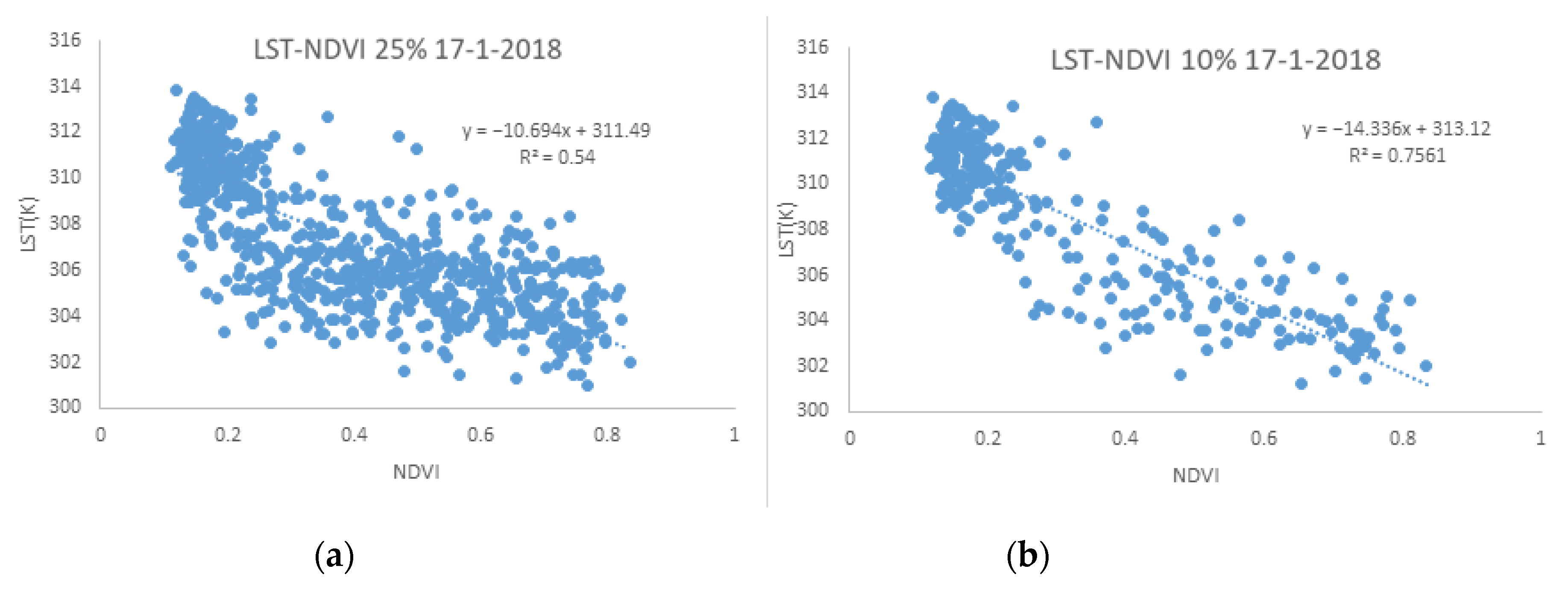
• Use linear regression instead of polynomial regression by assuming that polynomial is more sensitive for outliers.
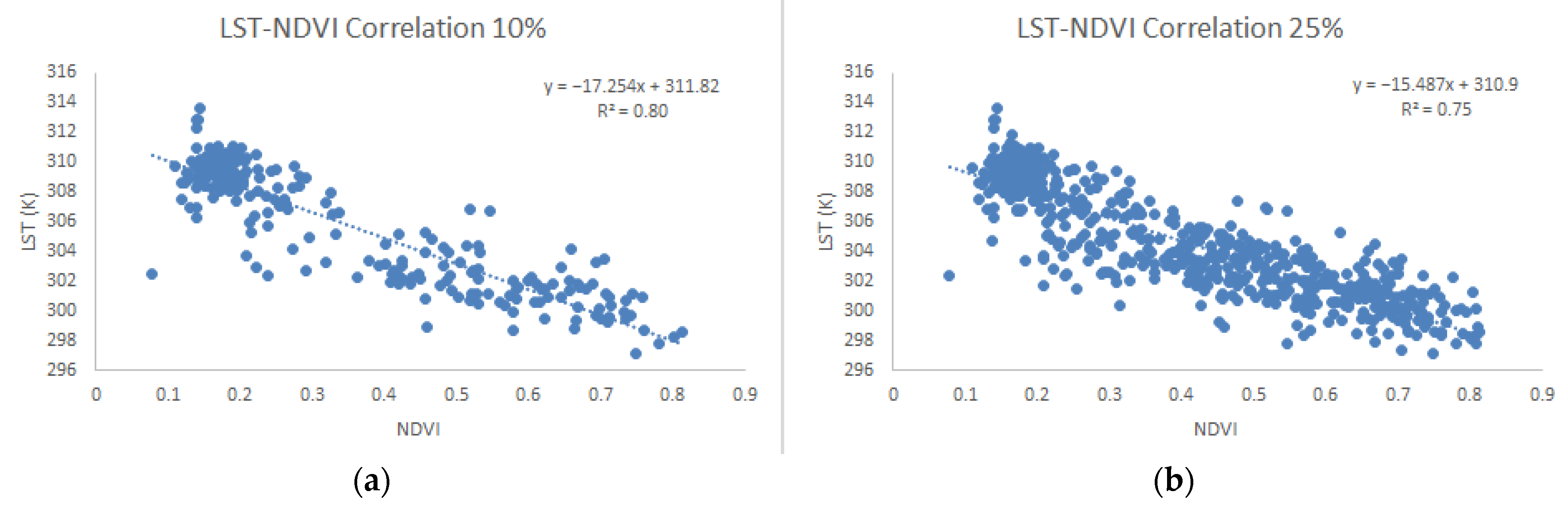
• Use 10% of the aggregated pixels instead of using 25% of the aggregated pixels assuming that based on the heterogeneity of the study area, the 10% of the aggregated pixels will give a stronger correlation between the NDVI and LST in the upper and lower tail in the distribution of the pixels.

The Validation

To validate this modification, we used the NDVI as shown in Figure 2 and LST calculated from the Landsat 8 image on the date 18 January 2018, and the steps are as follows:

• LST from the Landsat 8 was aggregated to a coarser resolution (1000 m).
• NDVI from Landsat 8 was aggregated to a coarse resolution (1000 m).
• The modification was applied to LST1000m and NDVI1000M to downscale LST to fine resolution.
• LSTnative was used to validate LSTdown.

Figure 2. NDVI derived from Landsat 8 18 January 2018.

Figure 2. NDVI derived from Landsat 8 18 January 2018.

The same modification was applied to MODIS (MOD11A1 V6. Product) for 37 images to create the time series.

2.3. Evapotranspiration Estimation

Evapotranspiration is the most important parameter in water balance in arid and semi-arid regions. Nonetheless, it is regarded as an element with poor temporal resolution despite its significance. As a result, its temporal resolution must be improved, especially if it is to be utilized for irrigation scheduling and planning. Therefore, it is necessary to downscale the land surface temperature since it is one of the most crucial factors in estimating evapotranspiration, which is the most dynamic parameter. In order to assess the ability of the LST downscaling to improve the temporal resolution of evapotranspiration, the Surface Energy Balance System model (SEBS) was used to estimate evapotranspiration. The original land surface temperature from Landsat 8, downscaled Landsat 8 land surface temperature, resampled MODIS land surface, and downscaled MODIS Land Surface Temperature were all considered to estimate evapotranspiration.

2.3.1. The Surface Energy Balance System

The Surface Energy Balance System (SEBS) model, designed by [35] to estimate evapotranspiration needs two types of data: The first group describes the physical properties of the land surface, including albedo, emissivity, temperature, fractional vegetation coverage, leaf area index, and the height of the vegetation (or roughness height). These data can be retrieved from satellite images. The second group describes the state of the atmosphere at a reference height, comprising air pressure, temperature, humidity, wind speed, downward solar radiation, and downward longwave radiation. These parameters can be determined from meteorological data measured directly or using a model. The data are also utilized to calculate roughness length for heat transfer and evaporative fraction.

SEBS is a physically based energy balance model that does not require prior knowledge of turbulent heat fluxes. To compute instantaneous relative evaporation, the model employs energy balance at wet and dry limiting conditions. The SEBS model is based on the energy balance equation (Equation (4)).

$${\mathit{R}}_{\mathit{n}}\mathbf{=}\mathsf{\lambda }\mathit{E}\mathbf{+}{\mathit{G}}_{\mathbf{0}}\mathbf{+}\mathit{H}$$

(4)

where: ${\mathit{R}}_{\mathit{n}}$ is the net radiation, λE is the turbulent latent heat flux (λ is the latent heat of vaporization and E is the actual evapotranspiration), ${\mathit{G}}_{\mathbf{0}}$ is the soil heat flux, and H is the turbulent sensible heat flux (All units are W·m⁻² or J·s⁻¹·m⁻²).

The calculation of net radiation flux on the land surface, R_n (W·m⁻²), is given by Equation (5).

$${\mathit{R}}_{\mathit{n}}\mathbf{=}\mathbf{\left(}\mathbf{1}\mathbf{-}\mathit{\alpha }\mathbf{\right)}{\mathit{R}}_{\mathit{s}\mathit{w}\mathit{d}}\mathbf{+}\mathit{\epsilon } {\mathit{R}}_{\mathit{l}\mathit{w}\mathit{d}}\mathbf{-}\mathit{\epsilon } \mathit{\sigma } {\mathit{T}}_{\mathbf{0}}{}^{\mathbf{4}}$$

(5)

where: α is the albedo (-), ${\mathit{R}}_{\mathit{s}\mathit{w}\mathit{d}}$ is the downward solar radiation (W·m⁻²), ε is the emissivity of the surface (-), ${\mathit{R}}_{\mathit{l}\mathit{w}\mathit{d}}$ is the downward longwave radiation (W·m⁻²), σ is the Stefan–Boltzmann constant (W·m⁻²·K⁻⁴), and ${\mathit{T}}_{\mathbf{0}}$ is the surface temperature (K).

The soil heat flux depends on land surface characteristics, soil water content, and other factors. Equation (6) gives the calculation of soil heat flux by the SEBS model:

$${\mathit{G}}_{\mathbf{0}}\mathbf{=}{\mathit{R}}_{\mathit{n}}\mathbf{\left(}{\mathit{\Gamma }}_{\mathit{c}}\mathbf{+}\mathbf{\left(}\mathbf{1}\mathbf{-}{\mathit{f}}_{\mathit{c}}\mathbf{\right)}\mathbf{·}\mathbf{\left(}{\mathit{\Gamma }}_{\mathit{s}}\mathbf{-}{\mathit{\Gamma }}_{\mathit{c}}\mathbf{\right)}\mathbf{\right)}$$

(6)

in which it is assumed that the ratio of soil heat flux to net radiation ${\mathit{\Gamma }}_{\mathit{c}}$ = 0.05 for full vegetation canopy and ${\mathit{\Gamma }}_{\mathit{s}}$ = 0.315 for bare soil. An interpolation is then performed between these limiting cases using the fractional canopy cover, ${\mathit{f}}_{\mathit{c}}$·(-).

The sensible heat flux is calculated using Equation (7).

$$\mathit{H}\mathbf{=}\mathbf{\left(}\mathbf{\left(}{\mathit{R}}_{\mathit{n}}\mathbf{-}{\mathit{G}}_{\mathbf{0}}\mathbf{\right)}\mathbf{-}\frac{\mathit{\rho }{\mathit{C}}_{\mathit{p}}}{{\mathit{r}}_{\mathit{e}\mathit{w}}}\mathbf{.}\frac{({\mathit{e}}_{\mathit{s}}\mathbf{-}\mathit{e})}{\mathit{\gamma }}\mathbf{\right)}\mathbf{/}\mathbf{1}\mathbf{+}\frac{∆}{\mathit{\gamma }}\mathbf{.}$$

(7)

${\mathit{R}}_{\mathit{n}}$ net radiation, ${\mathit{G}}_{\mathbf{0}}$= soil heat flux, $\mathit{\rho }$ = air density at constant pressure, ${\mathit{C}}_{\mathit{p}}$= specific heat of the air, $({\mathit{e}}_{\mathit{s}}\mathbf{-}\mathit{e})\mathbf{=}$ vapor pressure deficit of the air, $\mathit{\gamma }$ = psychrometric constant, ∆ = slope of the saturation vapor pressure.

We will use SEBS to estimate evaporation fraction by making energy balance at limiting cases at the dry limit and the wet limit as shown in Equation (8):

$${\mathsf{\Lambda }}_{\mathit{r}}\mathbf{=}\mathbf{1}\mathbf{-}\frac{\mathit{H}\mathbf{-}{\mathit{H}}_{\mathit{w}\mathit{e}\mathit{t}}}{{\mathit{H}}_{\mathit{d}\mathit{r}\mathit{y}}\mathbf{-}{\mathit{H}}_{\mathit{w}\mathit{e}\mathit{t}}}$$

(8)

where: the ${\mathit{H}}_{\mathit{w}\mathit{e}\mathit{t}}$ is sensible heat flux at the wet limit and ${\mathit{H}}_{\mathit{d}\mathit{r}\mathit{y}}$ sensible heat flux at the dry limit.

Since the ET ratio (evaporative fraction) Λ can be assumed constant during a day, the daily ET₂₄ (mm) can be estimated using the following equations:

$$\mathsf{\Lambda }\mathbf{=}\frac{\mathsf{\lambda }\mathit{E}}{{\mathit{R}}_{\mathit{n}}\mathbf{-}{\mathit{G}}_{\mathbf{0}}}\mathbf{=}\frac{ {\mathsf{\Lambda }}_{\mathit{r}}\mathbf{-}\mathsf{\lambda } {\mathit{E}}_{\mathit{w}\mathit{e}\mathit{t}}}{{\mathit{R}}_{\mathit{n}}\mathbf{-}\mathit{G}}\mathbf{.}$$

(9)

$${\mathit{E}}_{\mathit{d}\mathit{a}\mathit{i}\mathit{l}\mathit{y}}\mathbf{=}{\mathsf{\Lambda }}_{\mathbf{0}}^{\mathbf{24}}\mathbf{·}\mathbf{8.64}\mathbf{·}{\mathbf{10}}^{\mathbf{7}}\mathbf{·}\frac{{\mathit{R}}_{\mathit{N}}\mathbf{-}{\mathit{G}}_{\mathbf{0}}}{\mathsf{\lambda }\mathit{\rho }\mathit{w}}$$

(10)

where: ${\mathsf{\Lambda }}_{\mathit{r}}$ is relative evaporation, ${\mathsf{\Lambda }}_{\mathbf{0}}^{\mathbf{24}}$ daily evaporative fraction, $\mathit{\rho }\mathit{w}$ density of water measured in kilograms per cubic meter, and λ is the latent heat of vaporization.

2.3.2. Preparation of the Input Data for SEBS

To estimate actual evapotranspiration in SEBS the following data need to be prepared.

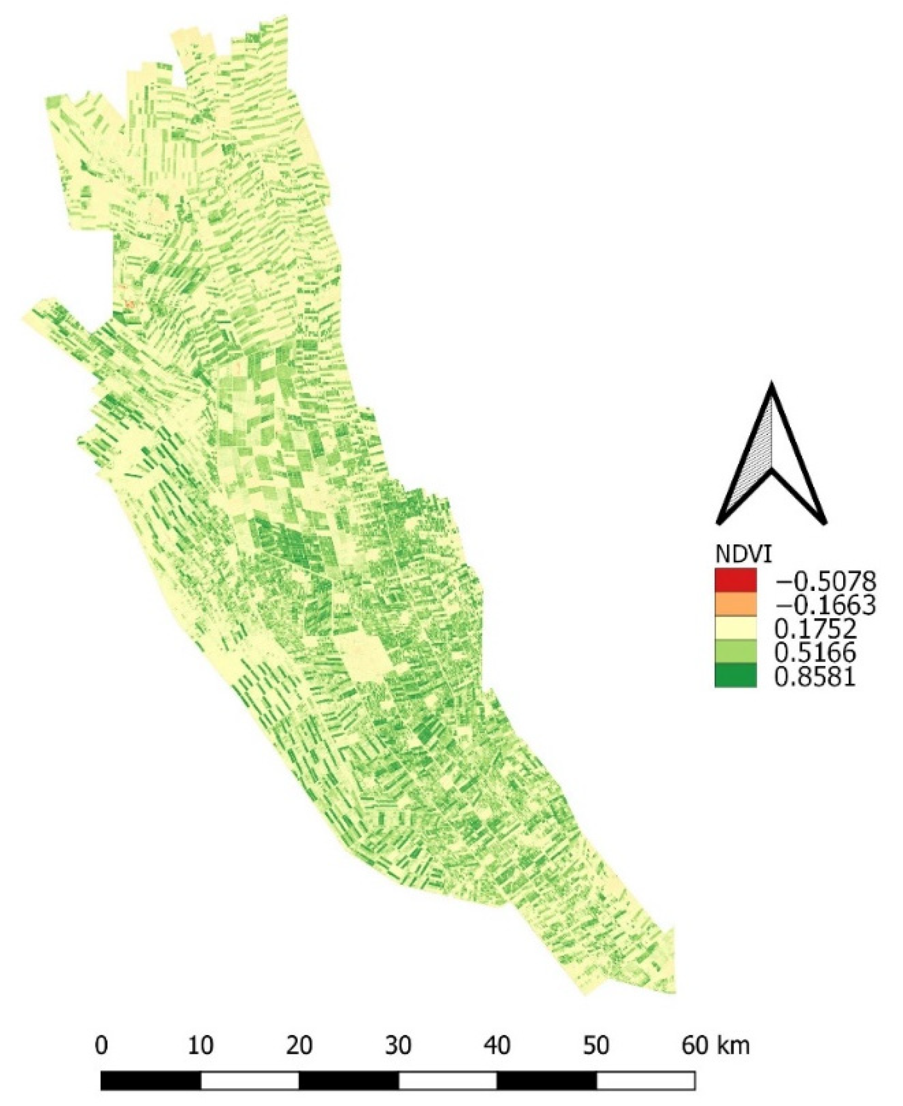
Normalized Different Vegetation Index (NDVI)

The NDVI was derived from Landsat 8 using Equation (11).

$$\mathit{N}\mathit{D}\mathit{V}\mathit{I}\mathbf{=}\frac{{\mathit{\rho }}_{\mathbf{5}}\mathbf{-}{\mathit{\rho }}_{\mathbf{4}}}{{\mathit{\rho }}_{\mathbf{5}}\mathbf{+}{\mathit{\rho }}_{\mathbf{4}}}$$

(11)

where: ${\mathit{\rho }}_{\mathbf{5}}$ is the reflectance in band 5, and ${\mathit{\rho }}_{\mathbf{4}}$ is the reflectance in band 4.

Fraction of Vegetation Cover (FVC)

FVC can be derived from NDVI maps (Equation (12)). In this study, FVC was estimated as proposed by [36] for fully vegetated cover and bare soil, as presented in Equation (12).

$$\mathit{F}\mathit{V}\mathit{C}\mathbf{=}\frac{\mathit{N}\mathit{D}\mathit{V}\mathit{I}\mathbf{-}\mathit{N}\mathit{D}\mathit{V}{\mathit{I}}_{\mathit{s}}}{\mathit{N}\mathit{D}\mathit{V}{\mathit{I}}_{\mathit{v}}\mathbf{-}\mathit{N}\mathit{D}\mathit{V}{\mathit{I}}_{\mathit{s}}}$$

(12)

where $\mathit{N}\mathit{D}\mathit{V}{\mathit{I}}_{\mathit{s}}$ represents the NDVI of bare soil, NDVI is the value of the actual pixel, and $\mathit{N}\mathit{D}\mathit{V}{\mathit{I}}_{\mathit{s}}$. corresponds to the NDVI value of the full vegetation canopy coverage.

Emissivity

The broad band land surface emissivity (ε) is calculated based on the FCV using Equation (13), which was introduced by [37].

$$\mathit{\epsilon }\mathbf{=}\mathbf{0.004}\mathbf{\times }\mathit{F}\mathit{V}\mathit{C}\mathbf{+}\mathbf{0.986}$$

(13)

Albedo

Albedo is the reflectance of a surface over a wide range of wavelengths. It indicates the reflected fraction of incoming radiation as a function of absorbed radiation. The broadband albedo was calculated using the Landsat 8 (OLI sensor) algorithm at the visible and NIR bands 2 to 7 in this study using Equation (14) [38].

$${\mathit{\alpha }}_{\mathit{O}\mathit{L}\mathit{I}}\mathbf{=}\mathbf{0.362}{\mathit{\rho }}_{\mathbf{2}}\mathbf{+}\mathbf{0.13}{\mathit{\rho }}_{\mathbf{4}}\mathbf{+}\mathbf{0.373}{\mathit{\rho }}_{\mathbf{5}}\mathbf{+}\mathbf{0.085}{\mathit{\rho }}_{\mathbf{6}}\mathbf{+}\mathbf{0.072}{\mathit{\rho }}_{\mathbf{7}}\mathbf{-}\mathbf{0.0018}$$

(14)

where: ${\mathit{\alpha }}_{\mathit{O}\mathit{L}\mathit{I}}$ is the shortwave albedo for Landsat, and ${\mathit{\rho }}_{\mathit{i}}$ is the reflectance of bands i = 2, 4, 5, 6, and 7.

Metrological Data

ERA5 provides data on planetary boundary layer height, incoming shortwave radiation, specific humidity, and pressure, while the ERAinterm data set provides data on sunlight hours.

The air temperature and wind speed inputs will be obtained from the New Halfa meteorological station. These data will be used as point measurements that will be considered representative of the study area since it is a flat area with a gentle slope to the north.

2.3.3. Retrieval of Actual Evapotranspiration in SEBS

The evapotranspiration was calculated using the SEBS model extension, which is included in the ILLWIS program. Daily evapotranspiration maps for 40 days were produced using the downscaled LST.

2.3.4. Data and Processing

The datasets were downloaded from open data sources, as shown in

Table 1. Data sources.

Data	Source	Spatial Resolution	Temporal Resolution
Landsat 8	https://espa.cr.usgs.gov/ordering/new/ (23 March 2020)	30 m	16 days
MODIS MOD11A1 V6	https://earthexplorer.usgs.gov/ (23 March 2020)	1 km	daily
NDVI	https://espa.cr.usgs.gov/ordering/new/ (23 March 2020)	30 m	16 days
Sunshine duration	https://apps.ecmwf.int/datasets/data/interim-full-daily/levtype=sfc/ (23 March 2020)	80 km	Daily
SRTM DEM	https://earthexplorer.usgs.gov/ (23 March 2020)	30 m	-
Other climatic data	https://www.ecmwf.int/en/forecasts/datasets/reanalysis-datasets/era5 (23 March 2020)	9 km	Daily

.

2.3.5. SEBS Validation

Since actual ET data were not available in the irrigated fields, the ETa estimated by SEBS was validated by comparing it to potential evapotranspiration estimated using crop coefficient and reference ET. This was based on the premise that under irrigated field conditions and adequate conditions for the ET, the crop’s potential ET is approximately equal to the crop’s actual evapotranspiration. Potential evapotranspiration (ETp) was estimated in the New halfa scheme as a product of kc and the reference evapotranspiration (ETo) values determined from the net radiation, relative humidity, air temperature, and wind speed using the Penman–Monteith method. The advantage of using remote sensing is that water used by the soil–water–vegetation system can be calculated directly without the need to quantify additional complicated hydrological processes.

2.3.6. Statistical Justification

The coefficient of determination, root mean square error (RMSE) Equation (15) and mean absolute error (MAE) Equation (16) are statistical measures of accuracy used to evaluate the performance of the downscaling modification and the evapotranspiration estimation.

$$\mathit{R}\mathit{M}\mathit{S}\mathit{E}\mathbf{=}\sqrt{\frac{{{\displaystyle \mathbf{\sum }}}_{\mathit{i}\mathbf{=}\mathbf{1}}^{\mathit{n}}{\mathbf{\left(}\mathit{L}\mathit{S}{\mathit{T}}_{\mathit{d}\mathit{o}\mathit{w}}\mathbf{-}\mathit{L}\mathit{S}{\mathit{T}}_{\mathit{n}\mathit{a}\mathit{t}\mathit{i}\mathit{v}\mathit{e}}\mathbf{\right)}}^{\mathbf{2}}}{\mathbf{2}}}$$

(15)

$$\mathit{M}\mathit{A}\mathit{E}\mathbf{=}\frac{{{\displaystyle \mathbf{\sum }}}_{\mathit{i}\mathbf{=}\mathbf{1}}^{\mathit{n}}\mathbf{\left[}\mathit{a}\mathit{b}\mathit{s}\mathbf{\left(}\mathit{L}\mathit{S}{\mathit{T}}_{\mathit{d}\mathit{o}\mathit{w}}\mathbf{-}\mathit{L}\mathit{S}{\mathit{T}}_{\mathit{n}\mathit{a}\mathit{t}\mathit{i}\mathit{v}\mathit{e}}\mathbf{\right)}\mathbf{\right]}}{\mathit{n}}$$

(16)

where: $\mathit{L}\mathit{S}{\mathit{T}}_{\mathit{d}\mathit{o}\mathit{w}}$ is the modeled variable, $\mathit{L}\mathit{S}{\mathit{T}}_{\mathit{n}\mathit{a}\mathit{t}\mathit{i}\mathit{v}\mathit{e}}$ is the observed variable, and $\mathit{n}$ is the number of observations.

3. Results and Discussion

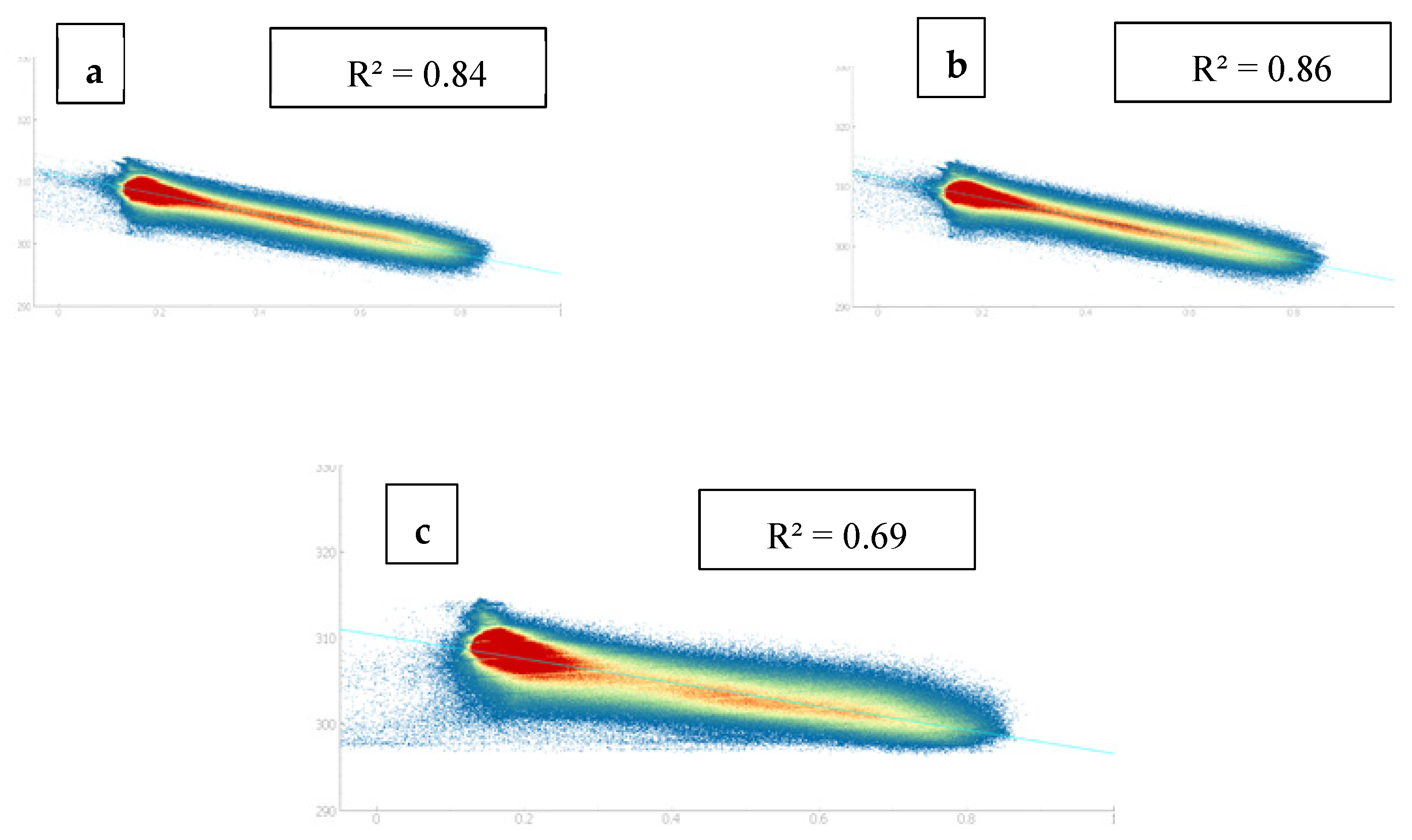
3.1. LST and NDVI Regression

The research was carried out during the growing season of the crops. (December–March). LST is inversely linked to NDVI in Figure 3, as was shown by, among others, [39,40].

Using a coefficient of determination (R²) indicates a stronger correlation between LST and NDVI, with values ranging from 0.86 to 0.84, all statistically significant. As shown in Figure 4, the results show an agreement when using 10% or 25% of the aggregated pixels for the downscaling process. Using 10% of the pixels gives a good result where R² values of both methods, 10% and 25% were (0.84, 0.86). However, it was higher than R² between LST and NDVI for the native LST R² (0.69). We attribute that to LST from the native Landsat image. It has a spatial resolution of 100 m and is resampled to 30 m resolution. As a result, the fields in the downscaled LST maps are more detailed.

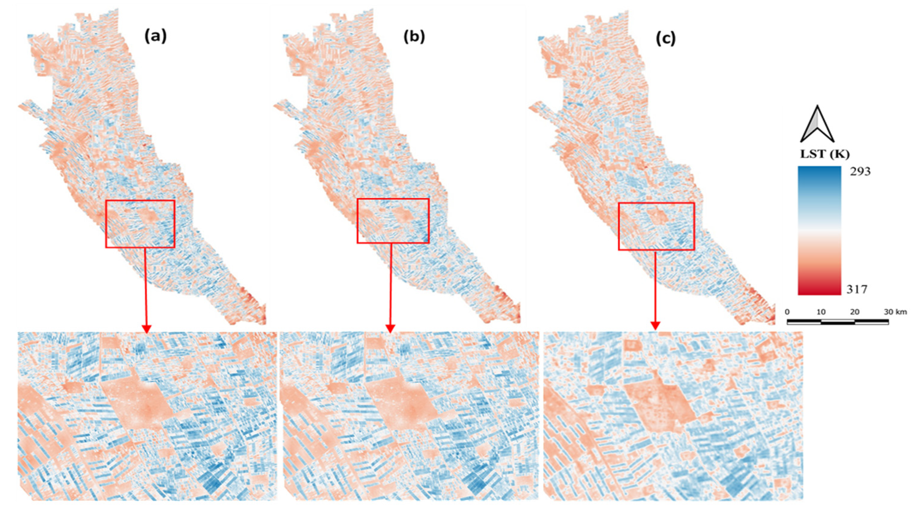
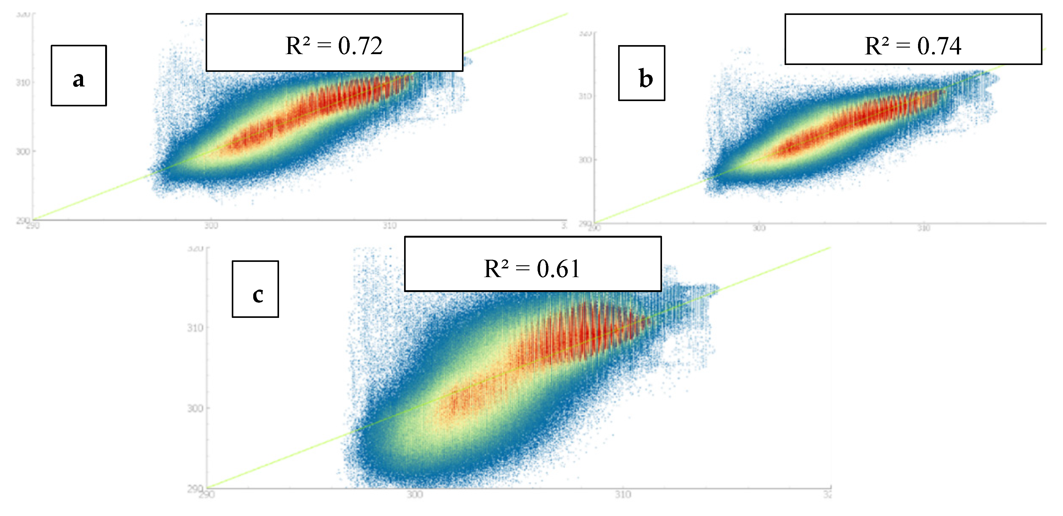
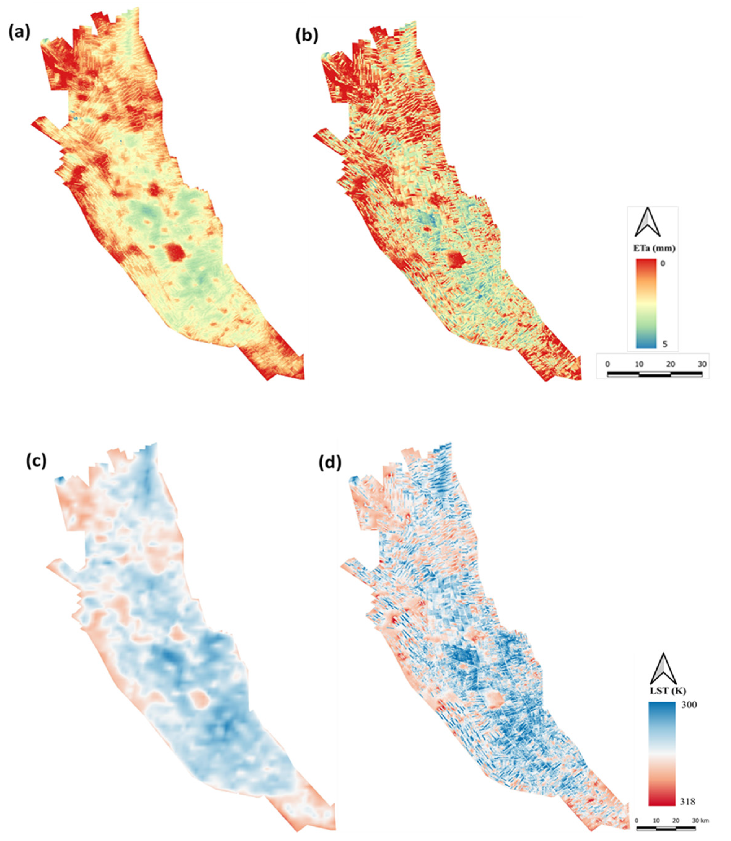
3.2. Effects of LST Downscaling on Landsat 8 Image

Figure 3 and Figure 4 show native LST (LSTnative) and downscaled LST (LSTdown) images of a subset of the study area with a target resolution of 30 m. Lower temperatures are associated with dense vegetation (and water surfaces), whereas higher temperatures are associated with urban and bare soil regions distant from cultivated land and dry sandy riverbanks. The mixed land cover zones have a moderate temperature. These downscaled LST patterns are identical to the original in contrast, tone, and saturation Figure 3 and Figure 5.

However, the simulated LST is unable to determine the temperature of the water bodies, which is why LSTdow is greater than LSTnative. Because the water surface has no relationship with NDVI, the error surface from visual interpretation exhibits greater error corresponding to a water body. These results agree with the results found by [20]. Similarly, bare soil shows higher error rates, followed by urban landscapes. Similarly, bare soil exhibits the greatest error, followed by urban settings. A minimum error was found in the cultivated area. According to [28,40], homogenous vegetated areas have a lower value of downscaling error due to the accurate fitting of regression models over such regions.

Table 2. Statistical analysis for the relation between native LST and LST25% and LST10%.

Method	Max ME	Min ME	Mean Error	RME
LST 25%	9.37	−5.12	−0.011	0.89
LST 10%	10.16	−5.63	−0.012	0.98

shows the minimum, maximum, (Root Mean Square Error) RMSE, and (Mean Error) ME calculated from the difference between LSTdown and LSTnative. The minimum and maximum temperature values of LSTdown surfaces also agree with the LSTnative.

The minimum and maximum temperatures are very close to LSTnative at 10% and 25% of the data used for correlation, and the coefficient of determination (R²) when using 10% is 0.72. It is R² = 0.74 for the 25%. Ref. [13] found that the RMSE increased with the increase of the target resolution, which is an indicator of decreasing accuracy in the finer resolution as shown in Figure 6. The same result was observed by [28]. This is because of the increasing degree of subpixel variability. Based on this statistical analysis, this modification yields superior results since the other scientists were attempting to achieve coarser resolution than the goal of this research.

The DisTrad method recommended the use of 25% of aggregated pixels with the lowest coefficient of variation for defining the regression equation. Still, in the case of the heterogonous area, like the small fields in the study region, the coefficient of determination can be low due to the high number of mixed pixels. To overcome these problems, 10% of the aggregated pixels with the lowest coefficient of variation were used to fit the correlation.

The result shows that using 10% of the data with the lowest coefficient of variation gave a higher correlation than using 25% of the data with the lowest coefficient of variation, which R² was 0.75 and 0.80 for LST25% and 10%, respectively, as shown in Figure 6.

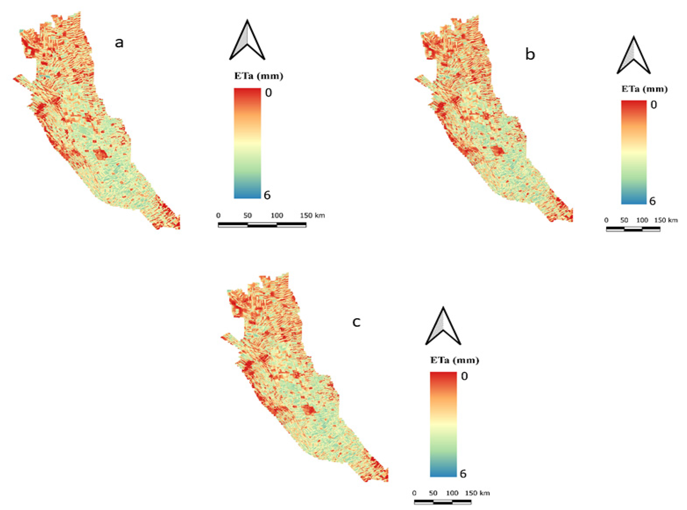
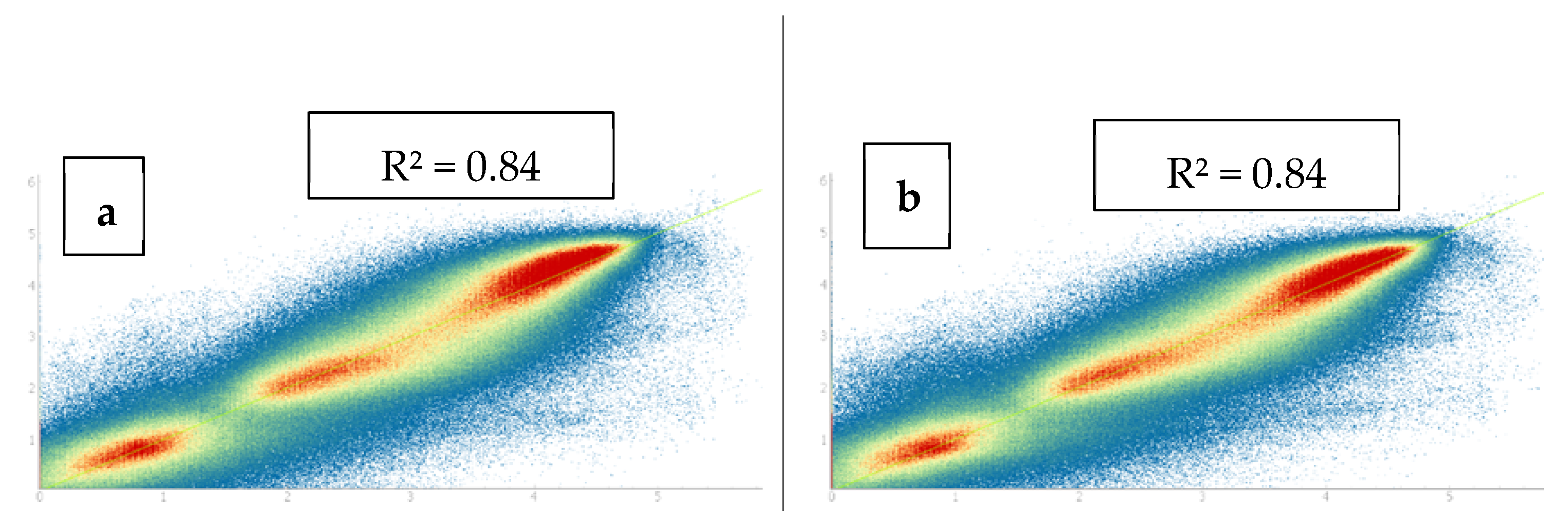
3.3. Effects of Downscaling LST on ET_a Estimation

Concerning the effect of downscaling the land surface temperature on evapotranspiration estimation, we found that the downscaling using only 10% of the pixels results in a good correlation due to the high degree of convergence between the results from these two methods and the native Land Surface Temperature, where the coefficient of determination for both methods 10% and 25% were (84.5 and 84.1) and yielded an average RMSE (0.3 and 0.28 mm/day, respectively). The evapotranspiration maps produced using downscaled land surface temperature had a higher spatial resolution than those produced using native land surface temperature, as the details and boundaries of small fields are more accurate on these maps than on the maps produced using native land surface temperature, as shown in Figure 7 and Figure 8 [19] produced RMSE in the similar range of 0.16 and TsHARP = 0.55 mm/day using the non-linear disaggregation approach (NL-DisTrad).

3.4. Application of Downscaling Model on MODIS Data

After applying the downscaling model to both methods on the Landsat image, the downscaled surface temperature gives reasonable results at an accuracy of 30 m. MODIS data at 1000 m spatial resolution is available with a temporal resolution of one day (17 January 2018). The optical data of 250 m and 500 m are also available with temporal resolution every day, but the obstacle to using optical data from MODIS is that the results obtained from these sensors are not suitable for use in the water management process for small fields due to their poor spatial resolution. Therefore, it is preferable to use optical data from Landsat because they have a high spatial resolution of 30 m. We find that the NDVI from a single Landsat image is suitable for the downscaling model of more than one MODIS image, where it is assumed that the NDVI does not change significantly during this period. Therefore, the NDVI produced by Landsat was used to model the land surface temperature with MODIS products. By using the visual interpretation of the maps resulting from the downscaling process, we find that the downscaling process gives the same effect that appeared when the model was used on the image of Landsat, where the downscaling led to the clarification of the parameters of small fields and the indication of their limits. We also find that the land surface temperature pattern follows the NDVI pattern in terms of density. The low temperatures are in the fields with high NDVI density, while the high temperatures appear in the fields with low NDVI density or in the bare soil and urban areas. This method was followed due to the lack of land surface temperature data for the surface on that day to be taken as a reference. As several scientists indicated, we needed data taken on the same day to be considered a reference and used to validate these results [41,42]. Some scientists pointed out that the difference in the sensors could also affect the results [20]. On the other hand, when comparing the modifications applied to the Kustas method, the parameterization improves the correlation between the vegetation cover and LST, as shown in Figure 9 (a) NDVI and LST25% correlation, (b) NDVI and LST10% correlation and Figure 10 ETa (a) derived from MODIS LST resampled and (b) downscaled, respectively. MODIS LST (c) resampled and (d) downscaled. However, when we tested the MODIS land surface temperature using Landsat 8 data on 18 January 2018, the findings revealed an average RMSE of 1.3 K.

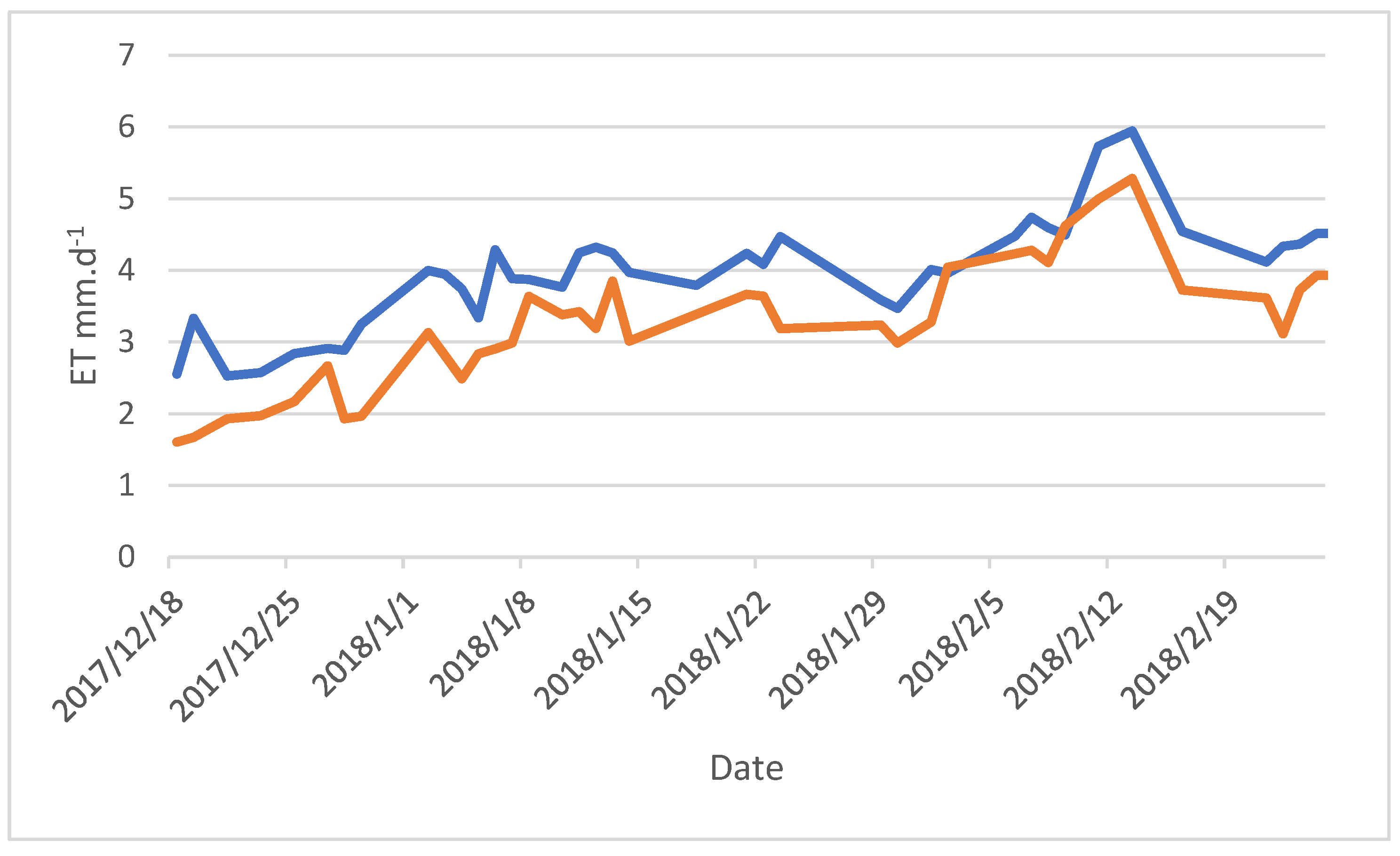
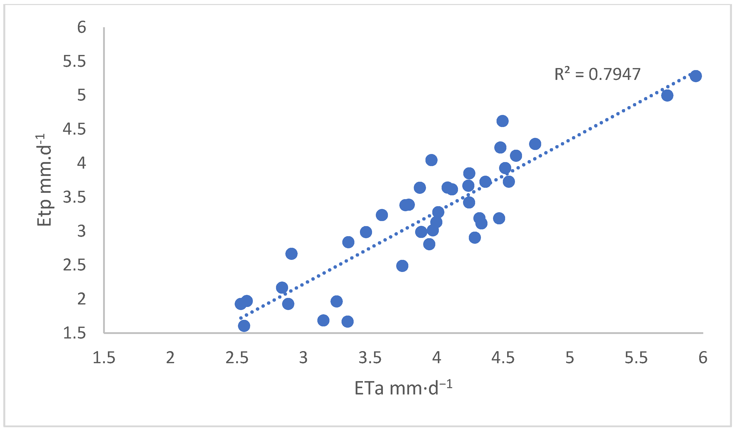
3.5. Model Validation

To demonstrate that downscaling improves the temporal resolution of evapotranspiration, 40 downscaled land surface temperature maps were used to estimate actual evapotranspiration for wheat crops from 18 December 2017 to 24 February 2018. Eight pixels from eight different fields were chosen, and the mean calculated for these pixels was compared to potential evapotranspiration. Figure 11 and Figure 12 shows the daily evapotranspiration (mm·day⁻¹) calculated using the SEBS approach, ranging from 1.5 mm·d⁻¹ at the start of the season to 5.2 mm·d⁻¹ in the mid-season.

The result compared to potential evapotranspiration ETp was estimated from reference evapotranspiration based on the metrological parameters and crop coefficient. As illustrated in Figure 11, SEBS underestimated evapotranspiration. However, as shown in Figure 11, there was a strong correlation between the two products, with R² = 79. Figure 12, on the other hand, depicts realistic trends in the accuracy of ETa generated from SEBS. Figure 12 likewise depicts steady trends in ETa over the course of the wheat growing season. From the above-mentioned results, we can indicate that the LST downscaling improves the temporal evapotranspiration resolution.

4. Conclusions

This article demonstrates how to reparametrize the DisTrad technique for downscaling land surface temperature over small fields in arid and semi-arid environments by addressing the relationship between land surface temperature and vegetation cover at high resolution. The study area is described as a mixed land cover class. It has a variety of distinct land cover types (dense vegetation, medium vegetation, low vegetation, bare soil, urban areas, and water). Due to the complexity of the vegetation cover in this region, where all the fields have a small area, it is difficult to find pixels with a 1 km resolution with dense vegetation cover except in a few pixels. As a result, it was suggested that we use a smaller number of pixels for the downscaling process. It was also suggested to use a linear regression instead of a second-order polynomial since the linear regression is more robust at the edges of the curve and avoids the extreme values resulting from the second-order polynomial. Good results were achieved, which can improve the downscaling process in regions with characteristics like the study area. Compared to the polynomial regression, the LST linear regression resulted in an R² = 0.74, 0.72 for 25% and 10%, respectively.

The downscaled land surface temperature evolved into the Surface Energy Balance system module to estimate the actual evapotranspiration at higher temporal resolutions (30 m). This parametrization was applied to the DisTrad method to improve the temporal and spatial resolution of LST and ET, giving RMSE 0.3 and 0.28 mm/day, respectively. Previous studies by [19] used the non-linear method (NL-DisTrad) to aggregate land surface temperature and compared it with the TsHARP method, and integrated it into the model to estimate ET_a. Both methods yielded RMSE = 0.16 for (NL-DisTrad) and 0.55 mm/day for TsHARP another research done by [43] used g the Jarvis model to simulate surface resistance for downscaling evapotranspiration in Zhangye Oasis the result obtained in this work generated RMSE = 0.50 mm/day. Finally, we may extrapolate from the aforementioned findings that this change can enhance and provide dependable Eta maps for irrigation scheduling and agricultural planning. Based on the above-mentioned results, we can conclude that the DisTrad modification has improved the evapotranspiration spatial and temporal resolution.

References

1. Bah, A.R.; Norouzi, H.; Prakash, S.; Blake, R.; Khanbilvardi, R.; Rosenzweig, C. Spatial Downscaling of GOES-R Land Surface Temperature over Urban Regions: A Case Study for New York City. Atmosphere 2022, 13, 332. [Google Scholar] [CrossRef]
2. Wang, S.; Luo, Y.; Li, X.; Yang, K.; Liu, Q.; Luo, X.; Li, X. Downscaling Land Surface Temperature Based on Non-Linear Geographically Weighted Regressive Model over Urban Areas. Remote Sens. 2021, 13, 1580. [Google Scholar] [CrossRef]
3. Song, C.; Hu, G.; Wang, Y.; Qu, X. Downscaling ESA CCI Soil Moisture Based on Soil and Vegetation Component Temperatures Derived From MODIS Data. IEEE J. Sel. Top. Appl. Earth Obs. Remote Sens. 2022, 15, 2175–2184. [Google Scholar] [CrossRef]
4. Yang, Y. A Scale-Separating Framework for Fusing Satellite Land Surface Temperature Products. Remote Sens. 2022, 14, 983. [Google Scholar] [CrossRef]
5. Pan, X.; Zhu, X.; Yang, Y.; Cao, C.; Zhang, X.; Shan, L. Applicability of Downscaling Land Surface Temperature by Using Normalized Difference Sand Index. Sci. Rep. 2018, 8, 9530. [Google Scholar] [CrossRef] [Green Version]
6. Zakšek, K.; Oštir, K. Downscaling land surface temperature for urban heat island diurnal cycle analysis. Remote Sens. Environ. 2012, 117, 114–124. [Google Scholar] [CrossRef]
7. Zhan, W.; Chen, Y.; Zhou, J.; Wang, J.; Liu, W.; Voogt, J.; Zhu, X.; Quan, J.; Li, J. Disaggregation of remotely sensed land surface temperature: Literature survey, taxonomy, issues, and caveats. Remote Sens. Environ. 2013, 131, 119–139. [Google Scholar] [CrossRef]
8. Li, W.; Wu, H.; Duan, S.B.; Li, Z.L.; Liu, Q. Selection of Predictor Variables in Downscaling Land Surface Temperature using Random Forest Algorithm. In Proceedings of the 2019 IEEE International Geoscience and Remote Sensing Symposium, Yokohama, Japan, 28 July–2 August 2019; pp. 1817–1820. [Google Scholar]
9. Zhang, Z.; He, G.; Wang, M.; Long, T.; Wang, G.; Zhang, X. Validation of the generalized single-channel algorithm using Landsat 8 imagery and SURFRAD ground measurements. Remote Sens. Lett. 2016, 7, 810–816. [Google Scholar] [CrossRef]
10. Yu, P.; Zhao, T.; Shi, J.; Ran, Y.; Jia, L.; Ji, D. Data Descri tor Global spatiotemporally continuous MODIS land surface temperature dataset. Sci. Data 2022, 9, 143. [Google Scholar] [CrossRef]
11. Bartkowiak, P.; Castelli, M.; Notarnicola, C. Downscaling land surface temperature from MODIS dataset with random forest approach over alpine vegetated areas. Remote Sens. 2019, 11, 1319. [Google Scholar] [CrossRef] [Green Version]
12. Nugraha, A.S.A.; Gunawan, T.; Kamal, M. Downscaling land surface temperature on multi-scale image for drought monitoring. In Proceedings of the 6th Geoinformation Science Symposium 2019, Yogyakarta, Indonesia, 26–27 August 2019; p. 6. [Google Scholar]
13. Hutengs, C.; Vohland, M. Downscaling land surface temperatures at regional scales with random forest regression. Remote Sens. Environ. 2016, 178, 127–141. [Google Scholar] [CrossRef]
14. Peng, W.; Yuan, X.; Gao, W.; Wang, R.; Chen, W. Urban Climate Assessment of urban cooling effect based on downscaled land surface temperature: A case study for Fukuoka, Japan. Urban Clim. 2021, 36, 100790. [Google Scholar] [CrossRef]
15. U.S. Geological Survey. Landsat 8 Data Users Handbook; NASA: Washington, DC, USA, 2016; Volume 8, p. 97.
16. Guo, F.; Hu, D.; Schlink, U. Remote Sensing of Environment A new nonlinear method for downscaling land surface temperature by integrating guided and Gaussian filtering. Remote Sens. Environ. 2022, 271, 112915. [Google Scholar] [CrossRef]
17. Yang, Y.; Li, X.; Pan, X.; Zhang, Y.; Cao, C. Downscaling land surface temperature in complex regions by using multiple scale factors with adaptive thresholds. Sensors 2017, 17, 744. [Google Scholar] [CrossRef] [PubMed] [Green Version]
18. Pu, R. Assessing scaling effect in downscaling land surface temperature in a heterogenous urban environment. Int. J. Appl. Earth Obs. Geoinf. 2020, 96, 102256. [Google Scholar] [CrossRef]
19. Bindhu, V.M.; Narasimhan, B.; Sudheer, K.P. Development and verification of a non-linear disaggregation method (NL-DisTrad) to downscale MODIS land surface temperature to the spatial scale of Landsat thermal data to estimate evapotranspiration. Remote Sens. Environ. 2013, 135, 118–129. [Google Scholar] [CrossRef]
20. Mukherjee, S.; Joshi, P.; Garg, R. A comparison of different regression models for downscaling Landsat and MODIS land surface temperature images over heterogeneous landscape. Adv. Space Res. 2014, 54, 655–669. [Google Scholar] [CrossRef]
21. Sattari, F.; Hashim, M.; Pour, A.B. Thermal sharpening of land surface temperature maps based on the impervious surface index with the TsHARP method to ASTER satellite data: A case study from the metropolitan Kuala Lumpur, Malaysia. Measurement 2018, 125, 262–278. [Google Scholar] [CrossRef]
22. Atkinson, P.M. Downscaling in remote sensing. Int. J. Appl. Earth Obs. Geoinf. 2013, 22, 106–114. [Google Scholar]
23. Mao, Q.; Peng, J.; Wang, Y. Resolution Enhancement of Remotely Sensed Land Surface Temperature: Current Status and Perspectives. Remote Sens. 2021, 13, 1306. [Google Scholar] [CrossRef]
24. Kustas, W.P.; Norman, J.M.; Anderson, M.C.; French, A.N. Estimating subpixel surface temperatures and energy fluxes from the vegetation index-radiometric temperature relationship. Remote Sens. Environ. 2003, 85, 429–440. [Google Scholar] [CrossRef]
25. Yang, C.; Zhan, Q.; Lv, Y.; Liu, H. Downscaling Land Surface Temperature Using Multiscale Geographically Weighted Regression over Heterogeneous Landscapes in Wuhan, China. IEEE J. Sel. Top. Appl. Earth Obs. Remote Sens. 2019, 12, 5213–5222. [Google Scholar] [CrossRef]
26. Li, H.; Wu, G.; Xu, F.; Li, S. Landsat-8 and Gaofen-1 image-based inversion method for the downscaled land surface temperature of rare earth mining areas. Infrared Phys. Technol. 2021, 113, 103658. [Google Scholar] [CrossRef]
27. Xu, S.; Zhao, Q.; Yin, K.; He, G.; Zhang, Z.; Wang, G.; Wen, M.; Zhang, N. Spatial downscaling of land surface temperature based on a multi-factor geographically weighted machine learning model. Remote Sens. 2021, 13, 1186. [Google Scholar] [CrossRef]
28. Agam, N.; Kustas, W.P.; Anderson, M.; Li, F.; Neale, C.M. A vegetation index based technique for spatial sharpening of thermal imagery. Remote Sens. Environ. 2007, 107, 545–558. [Google Scholar] [CrossRef]
29. Ebrahimy, H.; Azadbakht, M. Downscaling MODIS land surface temperature over a heterogeneous area: An investigation of machine learning techniques, feature selection, and impacts of mixed pixels. Comput. Geosci. 2019, 124, 93–102. [Google Scholar] [CrossRef]
30. Laxén, J. Is Prosopis a Curse or a Blessing? An Ecological-Economic Analysis of an Invasive Alien Tree Species in Sudan; University of Helsinki, Viikki Tropical Resources Institute (VITRI): Helsinki, Finland, 2007. [Google Scholar]
31. Wallin, M. Resettled for Development—The Case of New Halfa Agricultural Scheme, Sudan; The Nordic Africa Institute: Uppsala, Sweden, 2014; Volume 59.
32. Srivastava, P.K.; Han, D.; Ramirez, M.R.; Islam, T. Machine Learning Techniques for Downscaling SMOS Satellite Soil Moisture Using MODIS Land Surface Temperature for Hydrological Application. Water Resour. Manag. 2013, 27, 3127–3144. [Google Scholar] [CrossRef]
33. Essa, W.; Verbeiren, B.; van der Kwast, J.; Batelaan, O. Improved DisTrad for downscaling thermal MODIS imagery over urban areas. Remote Sens. 2017, 9, 1243. [Google Scholar] [CrossRef] [Green Version]
34. Essa, W.; van der Kwast, J.; Verbeiren, B.; Batelaan, O. Downscaling of thermal images over urban areas using the land surface temperature-impervious percentage relationship. Int. J. Appl. Earth Obs. Geoinf. 2013, 23, 95–108. [Google Scholar] [CrossRef]
35. Su, Z. The Surface Energy Balance System (SEBS) for estimation of turbulent heat fluxes. Hydrol. Earth Syst. Sci. 2002, 6, 85–100. [Google Scholar] [CrossRef]
36. Jiménez-Muñoz, J.C.; Sobrino, J.A.; Plaza, A.; Guanter, L.; Moreno, J.; Martínez, P. Comparison between fractional vegetation cover retrievals from vegetation indices and spectral mixture analysis: Case study of PROBA/CHRIS data over an agricultural area. Sensors 2009, 9, 768–793. [Google Scholar] [CrossRef] [PubMed]
37. Sobrino, J.A.; Jiménez-Muñoz, J.C.; Paolini, L. Land surface temperature retrieval from LANDSAT TM 5. Remote Sens. Environ. 2004, 90, 434–440. [Google Scholar] [CrossRef]
38. Liang, S.; Shuey, C.J.; Russ, A.L.; Fang, H.; Chen, M.; Walthall, C.L.; Daughtry, C.S.T.; Hunt, R., Jr. Narrowband to broadband conversions of land surface albedo: II. Validation. Remote Sens. Environ. 2003, 84, 25–41. [Google Scholar] [CrossRef]
39. Karnieli, A.; Bayasgalan, M.; Bayarjargal, Y.; Agam, N.; Khudulmur, S.; Tucker, C.J. Comments on the use of the Vegetation Health Index over Mongolia. Int. J. Remote Sens. 2006, 27, 2017–2024. [Google Scholar] [CrossRef]
40. Jeganathan, C.; Hamm, N.; Mukherjee, S.; Atkinson, P.; Raju, P.; Dadhwal, V. Evaluating a thermal image sharpening model over a mixed agricultural landscape in India. Int. J. Appl. Earth Obs. Geoinf. 2011, 13, 178–191. [Google Scholar] [CrossRef]
41. Njuki, S.M. Assessment of Irrigation Performance by Remote Sensing in the Naivasha Basin, Kenya. Master’s Thesis, University of Twente, Enschede, The Netherlands, February 2016; p. 65. [Google Scholar]
42. Kyalo, D.K. Sentinel-2 and MODIS Land Surface Temperature-Based Evapotranspiration for Irrigation Efficiency Calculations. Master’s Thesis, University of Twente, Enschede, The Netherlands, February 2017; p. 50. [Google Scholar]
43. Tan, S.; Wu, B.; Yan, N. A method for downscaling daily evapotranspiration based on 30-m surface resistance. J. Hydrol. 2019, 577, 123882. [Google Scholar] [CrossRef]
Figure 1. Location map describes the study area.
Ijgi 11 00327 g001
Figure 3. (a,b) Correlation between the NDVI and LST daily average for 10% and 25% methods, respectively.
Ijgi 11 00327 g003
Figure 4. (a) LST Landsat10%, (b) LST Landsat 25%, and (c) LST Landsat native.
Ijgi 11 00327 g004
Figure 5. (ac) Scatter plot for the relation between NDVI and LST 10%, LST 25%, and LST native, respectively.
Ijgi 11 00327 g005
Figure 6. (ac) Scatter plot between native LST with LST10%, LST 25%, and LST25% polynomial, respectively.
Ijgi 11 00327 g006
Figure 7. (ac) Eta for native LST, LST 10%, and LST 25%, respectively.
Ijgi 11 00327 g007
Figure 8. Correlation scatter plot of (a) ETa (LST native) against ETa (LST10%) and (b) ETa (LST native) against ETa (LST25%).
Ijgi 11 00327 g008
Figure 9. (a) NDVI and LST25% correlation, (b) NDVI and LST10% correlation.
Ijgi 11 00327 g009
Figure 10. ETa (a) derived from MODIS LST resampled and (b) downscaled, respectively. MODIS LST (c) resampled and (d) downscaled.
Ijgi 11 00327 g010
Figure 11. Comparison between daily ETp (blue line) VS. ETa (red line) for 18 August 2017 to 24 February 2018.
Ijgi 11 00327 g011
Figure 12. Correlation between ETp and ETa (mm·d−1).
Ijgi 11 00327 g012