Fast Inversion of Air-Coupled Spectral Analysis of Surface Wave (SASW) Using in situ Particle Displacement

Abstract

Spectral Analysis of Surface Wave (SASW) is widely used in nondestructive subsurface profiling for geological sites. The air-coupled SASW is an extension from conventional SASW methods by replacing ground-mounted accelerometers with non-contact microphones, which acquire a leaky surface wave instead of ground vibration. The air-coupled SASW is a good candidate for fast inspection in shallow geological studies. Especially for pavement maintenance, minimum traffic interference might be induced. One issue that restrains SASW from fast inspection is the traditional slow inversion which relies on guess-and-check iteration techniques including a forward analysis. In this article, a fast inversion analysis algorithm is proposed to estimate the shear velocity profile without performing conventional forward simulation. By investigating the attenuation of particle displacement along penetrating depths, a weighted combination relationship is derived to connect the dispersion curve with the shear velocity profile directly. Using this relationship, the shear velocity profile could be estimated from a given/measured dispersion curve. The proposed procedure allows the surface wave-based method to be fully automatic and even operated in real-time for geological site and pavement assessment. The method is verified by the forward analysis with stiffness matrix method. It is also proved by comparing with other published results using various inversion methods.

1. Introduction

Many methods are being developed and utilized for the subsurface sensing, including Impact Echo (IE), Impulse Response (IR), Ground Penetrating Radar (GPR), Chain-Drag, and Spectral Analysis of Surface Waves (SASW). IE is able to identify the debonding and properties of shallow top layers [1]. IR can test the overall dynamic stiffness/mobility of the entire pavement structure [2]. GPR is best for locating metal materials, such as reinforcement rebars [3]. Chain-Drag can find debonded areas by listening for hollow sounds [4]. The SASW and its related methods are very popular for their capability of estimating the thickness and elastic modulus of subsurface layers [5,6].

Since first proposed in 1980s [6,7], the SASW has been widely applied in the geological field tests to estimate the underground soil profile without coring or opening the ground [8]. It utilizes the dispersion features of the surface wave that propagates horizontally in the soil when it is subject to an impact load. The dispersion curve represents the relationship between the wave speed, wave length and frequency. Once the dispersion curve is obtained from the test data, the layer profile, and shear velocities can be estimated by inversion algorithms. Extensive researches have been made to improve the accuracy and efficiency during the inversion procedure. Among those, the stiffness matrices method was widely used to supply the forward simulation for inversion analysis [9]. In recent years, SASW has been extended to investigate pavement systems [10,11] and concrete structures [12]. Some other methods were successfully developed based on the same principle of SASW. Among those, the Multichannel Analysis of Surface Wave (MASW) method uses multiple sensors to record the complete wave field and resolve the different wave modes [13].

Despite these exciting achievements of SASW methods, the state of the art of the surface wave-based methods are still limited as off-line low-efficiency test technique due to the expertise involved iterative algorithms and contact sensing. The low speed and traffic interruption hinders its implementation in the pavement inspection. Recently, attempts were made to improve the testing speed by using non-contact sensors, the microphones, to replace the traditional contact sensors, accelerometers, or geophones [14], in which the leaky surface wave collected by the microphones is used to analyze the dispersion. Mobile testing concept was also investigated to perform fast testing on concrete slabs by Ryden et al. [15], which inspired the community for efforts on non-contact surface wave testing.

One major issue that confines the efficiency of the SASW family methods is the iterative inversion process, which is usually time consuming and requires human expertise to set the initial and adjusted values of the elastic modulus profile. Consequently, the SASW method is basically limited as a point-to-point posted-processed stationary test. Researchers are seeking faster and automated inversion analysis algorithms to enhance its efficiency. An algorithm was developed in 1995 to construct the dispersion curve rapidly through fitting a complex-valued curve to the phase information of the cross power spectra using coherence function as weighting function [16]. A Monte Carlo algorithm and the maximum likelihood method were chosen, respectively, to examine the possible solutions with minimal constraints and to estimate the uncertainties of the resulting model parameters [17]. In order to identify the predominant propagation modes easily, an inversion method based on the maximum vertical flexibility coefficient was introduced [18]. In addition, a new algorithm called peak-through and frequency-wave number (PT/FW) technique was developed in 2006 to determine the phase velocity more effectively instead of the traditional phase difference method [19]. Moreover, GA (genetic algorithm)-based inversion [20] and combination of genetic and linearized algorithms in a two-step joint inversion [21] were also employed in recent years. However, all these improvements only modified the way of initializing and adjusting the assumed profile for quick convergence. The inversion still relies on the basic procedure of guessing first and checking with forward analysis. The fast simulated annealing (FSA) global search algorithm was another effort to minimize the difference between the measured shear velocity spectrum and that calculated from the theoretical layer model, including the field setup geometry [22]. This inversion brings new solutions but still somewhat suffers long-term iteration for acceptable accuracy. The simplified inversion method (SIM) for surface wave dispersion data was one more contribution to solve the inversion efficiently [23], which makes use of a penetration depth coefficient to provide shear wave velocity vs. depth profile.

In this paper, a fast inversion algorithm is proposed, utilizing the fundamental features of surface waves. In a homogeneous half-space, the particle displacement distribution characteristics along the penetrating depth are founded to dominate the relationship between shear velocity profile and the dispersion curve. The phase velocity at a certain wavelength is, therefore, expressed as a weighted combination of shear velocities within the penetrating depth using the normalized particle displacements as the weighting factors. Additionally, for layered half-space, the apparent wave mode would be the fundamental mode when the stiffness of layers is increasing from soft to hard with depth. In this case, the normalized particle displacements would still work as the weighting factors. A fast inversion algorithm is then established on the basis of this relationship. This proposed algorithm requires no manual input or adjustment of trial profiles, and therefore it is fully automated. Since no forward simulation such as the stiffness matrix method is required, the proposed method is fast enough for quasi real-time operation. The accuracy of this method is verified by stiffness matrix method and also by comparing the estimated shear velocity profiles with the results from other published methods.

2. Air-Coupled SASW

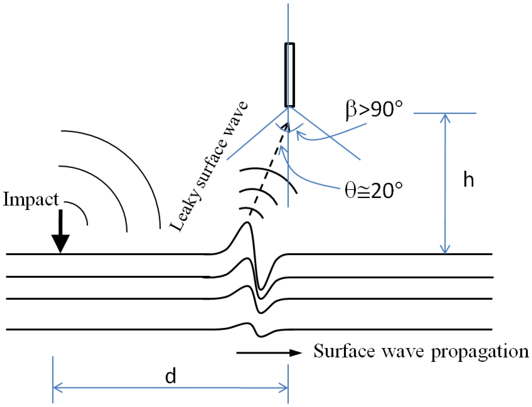
Considering a layered half-space subjects to an impact point load at the surface, as shown in Figure 1, in addition to P wave and shear wave propagate, the surface wave also propagates horizontally. In the air above the surface, the surface vibration acts as an acoustic source to radiate acoustic wave. This radiating acoustic wave is so called leaky surface wave. According to the Snell’s laws, the leaky angle θ is determined by:

$$\sin (\mathsf{\theta })=\frac{C_a}{C_R}$$

(1)

where, C_a and C_R are the acoustic wave velocity in the air and the surface wave (Rayleigh wave) velocity in the half-space (such as pavement). The C_a is about 340 m/s, and the C_R could be 1000 m/s for example. Therefore, the leaky angle θ ≈ 20°. The radiated surface wave can be detected with directional microphones, which usually have an effective angle of 100°.

Figure 1. Propagation of surface wave.

Figure 1. Propagation of surface wave.

By using the features of radiating surface wave, the SASW test can be performed with microphones, instead of accelerometers. Figure 2 shows a schematic configuration of this air-coupled SASW (or MASW) test. Two or more microphones are placed at a small distance above the ground and connected to the data acquisition device and computer. When an impact force is applied, the collected signal contains both the surface wave and the direct acoustic wave from the hammer. Under the condition that the microphones are near the surface and the shear velocity of the pavement is much larger than sound velocity, the direct acoustic wave from the hammer arrives to the microphone later than the surface wave. The difference of their arrival time can be calculated as:

$$\Delta t=\frac{\sqrt{d^2+h^2}}{C_a}-\frac{d-h\tan \mathsf{\theta }}{C_R}-\frac{h}{C_a\cos \mathsf{\theta }}$$

(2)

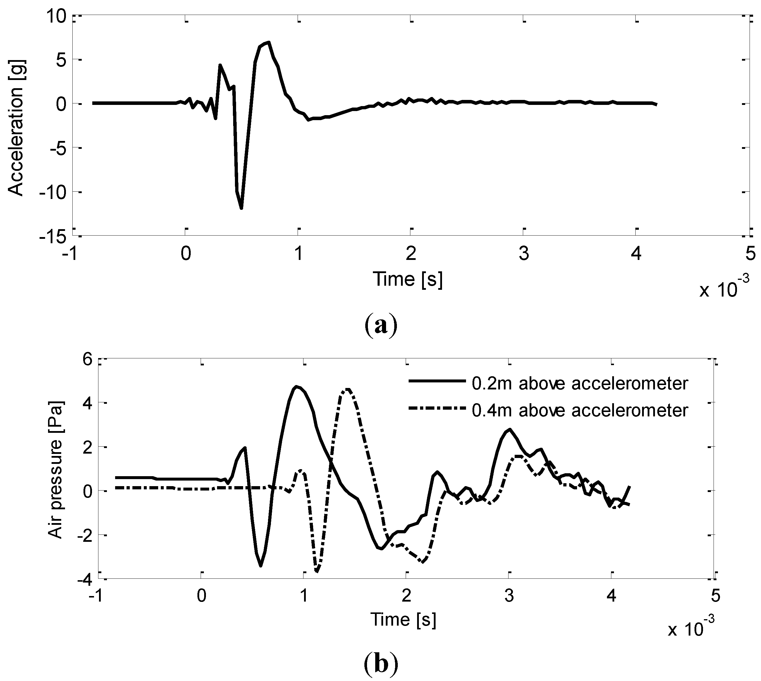
At a typical configuration with d = 0.5 m and h = 0.05 m, this time lag can be 1 ms. Therefore, the surface wave can be subtracted from the total signal by applying appropriate time window on the acquired data. Figure 3 shows an example of the surface wave measured by accelerometer (a) and the radiating surface wave measured by microphones (b). From the comparison, it can be seen that the first part of the microphone data arrives nearly at the same time and shows the similar feature as the accelerometer data. This part of data can be identified as radiating surface wave. The second part of the microphone data is regarded as noise because no signal is presented in the pairing accelerometer at the corresponding time.

Figure 2. Typical air-coupled SASW/MASW configuration.

Figure 2. Typical air-coupled SASW/MASW configuration.

Figure 3. (a) Sample data collected by accelerometer data; and (b) Sample data collected by microphone.

Figure 3. (a) Sample data collected by accelerometer data; and (b) Sample data collected by microphone.

The air-coupled SASW strategy can be extended to an air-coupled MASW by deploying a microphone array above the surface, as shown in Figure 2. The radiating surface wave can be extracted from the measured acoustic signals. The de-noising technologies, such as sound enclosures and digital filters could be employed to improve the implementation of air-coupled sensing through microphones. Forward dispersion analysis methods for traditional SASW can be used to analyze the radiating surface wave. Such methods can be found in many published literatures [6,8]. The proposed fast inversion methods are also compatible with air-coupled SASW strategy by microphone.

3. Particle Displacement of Surface Wave

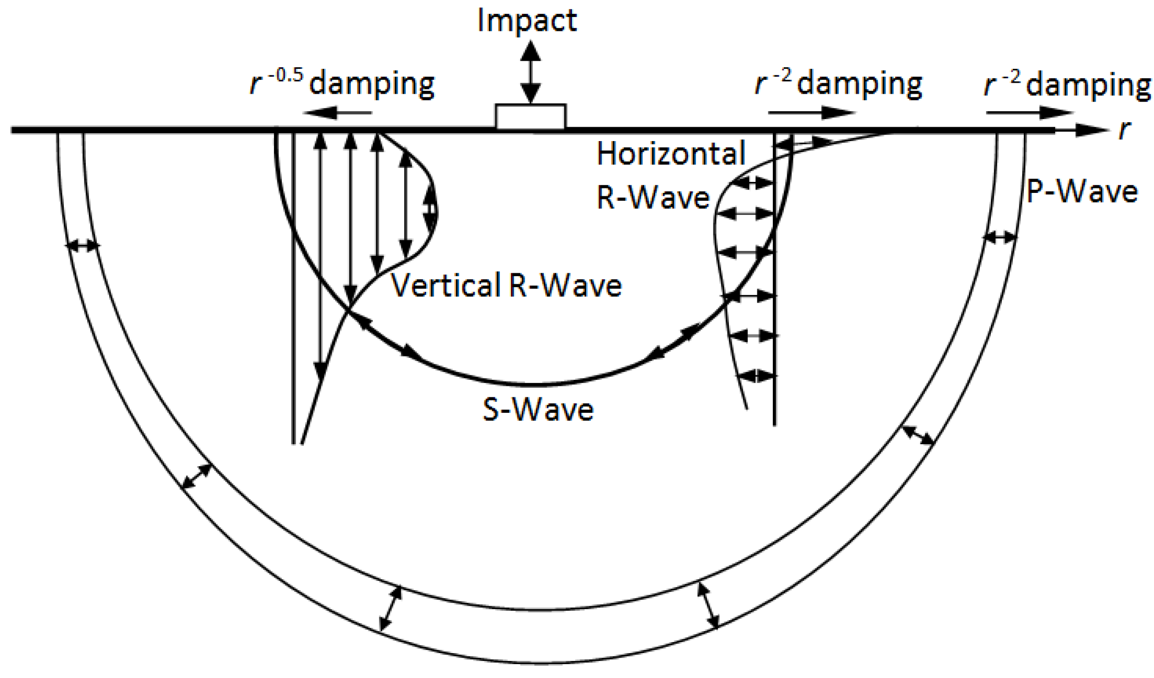
In this section, we briefly review properties of surface wave that are essential to the proposed inversion method. When a homogeneous half-space is subjected to a point force on the surface, three types of stress waves will be generated. They are two body waves: P-wave (compression wave) and S-wave (shear wave); and a surface wave (also called the Rayleigh wave or R-wave). Both body waves propagate inside the half-space but in perpendicular directions. The S wave owns vertical (S-V) and horizontal (S-H) components. The P-wave travels in the same direction with the particle vibration while the S-wave travels transversally. The R-wave, on the other hand, travels along the free surface of the half-space. Due to material damping, all three waves attenuate as they propagate, though at different rates. At the surface, the amplitudes of the P-wave and S-wave attenuate on the order of r⁻² (r is the radius from the source), while the surface wave attenuates much less on the order of r^−1/2. The surface wave is often used to measure material properties for the following reasons: (1) it is easily excited by surface impact; (2) it has a low attenuation; (3) it is also easily measured at the surface; and (4) it could be measured by radiating air-coupled waves. Figure 4 illustrates the pattern of these stress waves.

Figure 4. Distribution of stress waves from a vertical load on a homogeneous elastic half-space (after Richart et al. [24]).

Figure 4. Distribution of stress waves from a vertical load on a homogeneous elastic half-space (after Richart et al. [24]).

The relationship between the velocities of stress waves can be expressed with linear expressions as:

$$\frac{V_S}{V_P}=\sqrt{\frac{1-2\mathsf{\upsilon }}{2(1-\mathsf{\upsilon })}}$$

(3)

$$\frac{V_R}{V_S}\approx \frac{0.87+1.12\mathsf{\upsilon }}{1+\mathsf{\upsilon }}$$

(4)

where V_P, V_S, and V_R are phase speeds of P-wave, S-wave, and surface wave (R-wave), respectively; υ is the Poisson’s ratio.

Another basic feature of the surface waves is the shape of the wave-front. It has been discovered the surface wave propagates radially outward along a cylindrical wave front, while the P-wave and S-wave propagate along a hemispherical wave front, as shown in Figure 4. This means the surface wave within the penetrating depth propagates outward at the same velocity.

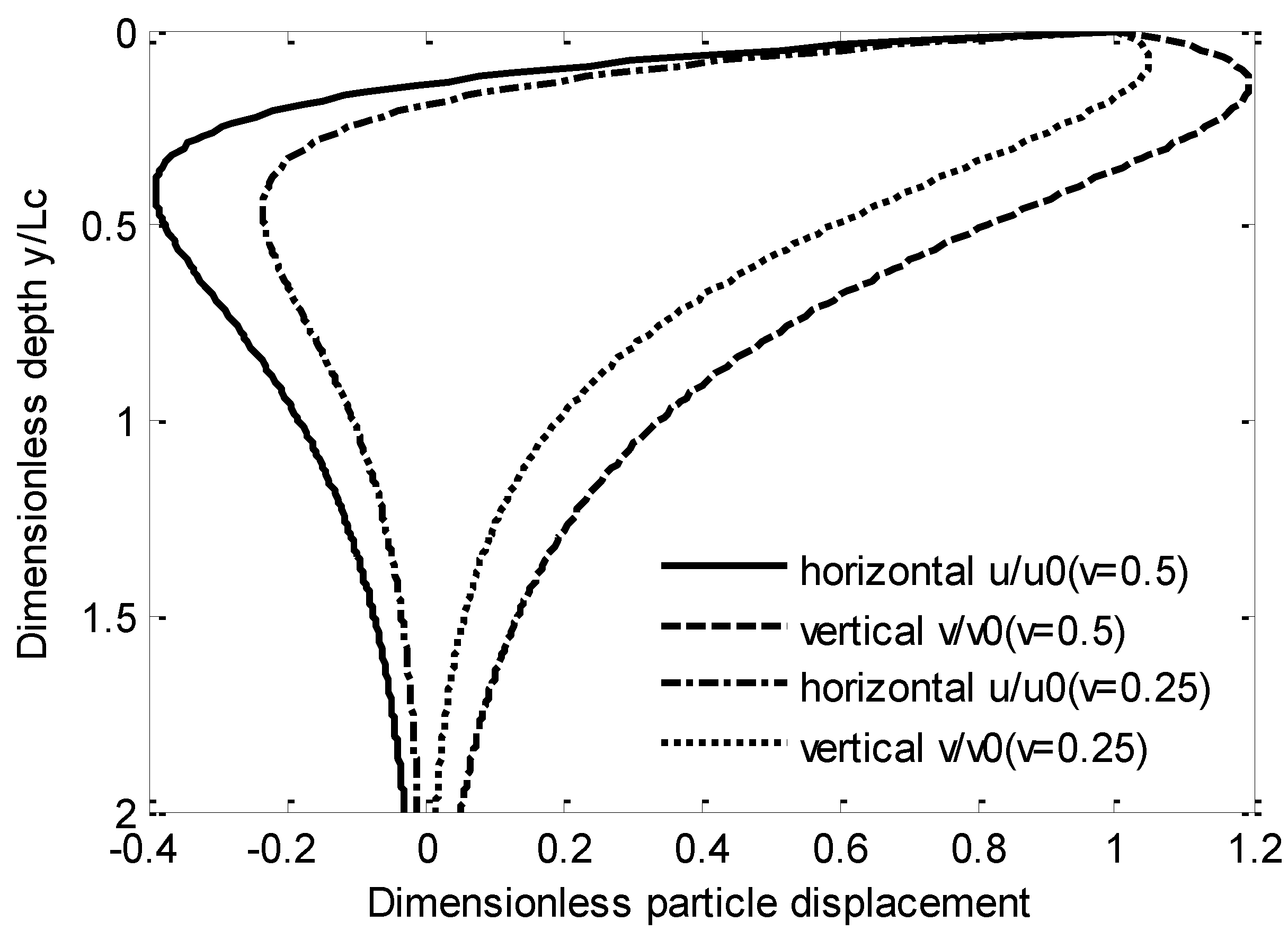
On the other hand, the particle motion of the surface wave varies along the penetrating depth and becomes small at the depth of approximately triple wavelengths. Barkan et al. gave the approximate solution to the particle displacement of surface wave along with the penetrating depth as [25]:

For Poisson’s ratio ν = 0.5:

$$\{\begin{array}{c}u(y)=\left(-0.1298e^{-\frac{2\mathsf{\pi }y}{L_c}}+0.0706e^{-\frac{\left(0.2958\right)2\mathsf{\pi }y}{L_c}}\right)\frac{P}{\mathsf{\mu }}\\ v(y)=\left(0.1298e^{-\frac{2\mathsf{\pi }y}{L_c}}-0.2387e^{-\frac{\left(0.2958\right)2\mathsf{\pi }y}{L_c}}\right)\frac{P}{\mathsf{\mu }}\end{array}$$

(5)

For Poisson’s ratio ν = 0.25:

$$\{\begin{array}{c}u(y)=\left(-0.2958e^{-\frac{(0.8474)2\mathsf{\pi }y}{L_c}}+0.1707e^{-\frac{\left(0.3933\right)2\mathsf{\pi }y}{L_c}}\right)\frac{P}{\mathsf{\mu }}\\ v(y)=\left(0.2507e^{-\frac{(0.8474)2\mathsf{\pi }y}{L_c}}-0.4341e^{-\frac{\left(0.3933\right)2\mathsf{\pi }y}{L_c}}\right)\frac{P}{\mathsf{\mu }}\end{array}$$

(6)

where u and v are the horizontal and vertical components of the amplitude of particle displacement, respectively; L_c is the wavelength; y is the depth; y/L_c is the dimensionless depth; µ is the Lamé coefficient (shear modulus); and P is the impact force.

When replacing u and v with the dimensionless displacement as u/u₀ and v/v₀ , respectively (u₀ and v₀ are the displacement at the surface), the distribution of particle displacement amplitude can be plotted in a graph with the dimensionless displacement vs. dimensionless depth, as shown in Figure 5. This ensures the effect on the particle displacement from the various Poisson’s ratio is negligible.

Figure 5. Distribution of particle displacement along with penetrating depth of surface wave (after Richart et al. [24]).

Figure 5. Distribution of particle displacement along with penetrating depth of surface wave (after Richart et al. [24]).

4. Fast Inversion Algorithm

4.1. Relationship between Phase Velocity and Shear Velocities of Layered System

For a layered ground system, the propagation of surface wave should keep in cylindrical wave front if the multimode effects are omitted while the fundamental mode is dominant. Therefore, it is reasonable to believe that a similar linear relationship still exists between the phase velocity and the shear velocities of the underground layers. Since the wave in the penetrated layers travel with the same wave number, it is probable that some kind of average of the shear velocities of these layers dominates the phase velocity. This assumption was confirmed by Xia et al. 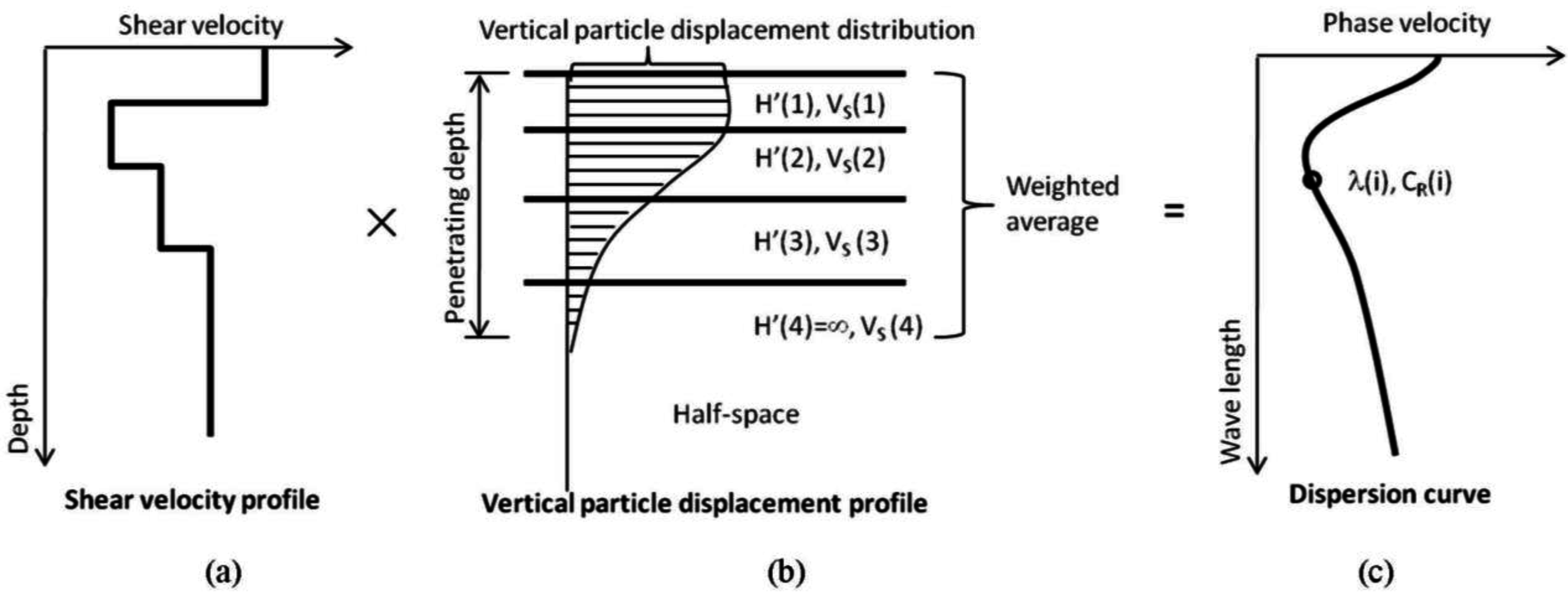[26] whose research discovered that compared with P-wave velocity, density, and layer thickness, the shear wave velocity is the dominant parameter influencing changes in Rayleigh-wave phase velocity in the high-frequency range (>5 Hz). Moreover, from the energy concept of view, the particle vibrating with larger displacement must contribute more to determine the velocity of the entire surface wave. Therefore, the distribution of particle displacement along penetrating depth would be chosen as the weighting factor of the averaging. Since only the vertical motion component of the surface wave is measured by SASW sensors, only the vertical component of particle displacement contributes to the weighting factors. Thus, a weighted averaging relationship is proposed herein to connect the phase velocity and the layer shear velocities directly as:

$$\{\begin{array}{ll}{V}_R(\mathsf{\lambda })=\frac{{\displaystyle {\sum }_1^n{H}^{\prime }(i)V_R^{\prime }(i)}}{{\displaystyle {\sum }_1^n{H}^{\prime }(i)}}& (7\text{a})\\ H^{\prime }(i)={\displaystyle {\mathsf{\int }}_{y_{i-1}}^{y_i}v(y)dy}& (7\text{b})\\ V_R^{\prime }(i)\approx \frac{0.87+1.12\mathsf{\upsilon }(i)}{1+\mathsf{\upsilon }(i)}{V}_S(i)& (7\text{c})\end{array}$$

where $V_R(\mathsf{\lambda })$ is the phase velocity of the surface wave as a function of wavelength λ; $H^{\prime }(i)$ is the equivalent thickness of layer i; $V_R^{\prime }(i)$ is the equivalent phase velocity at layer i; $v\left(y\right)$ is the vertical component of the particle displacement at the depth y; $\mathsf{\upsilon }\left(i\right)$ is the Poisson’s ratio of layer i; n are the total layers penetrated by the wavelength λ. Since $v\left(y\right)$ attenuates fast along the depth, choosing $y_n=2\mathsf{\lambda }$ can be fairly accurate according to Figure 5. Empirically, the total penetrating depth $y_n$ is about $0.3\mathsf{\lambda }$ to $0.4\mathsf{\lambda }$. Figure 6 illustrates the graphic relationship expressed in Equation (7a–c).

Figure 6. Relationship between shear velocity profile and dispersion curve for layered system; (a) Shear velocity profile; (b) Particle displacement; and (c) Dispersion curve.

Figure 6. Relationship between shear velocity profile and dispersion curve for layered system; (a) Shear velocity profile; (b) Particle displacement; and (c) Dispersion curve.

4.2. Inversion Algorithm

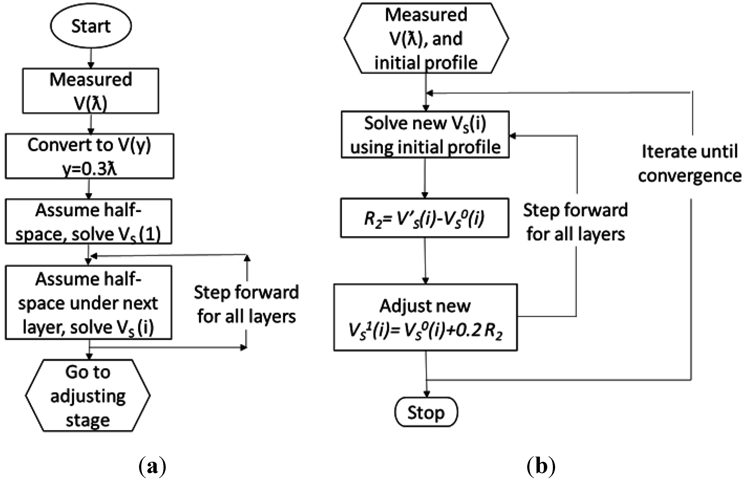
With the relationship revealed above, it is very easy to obtain the estimated phase velocity of a surface wave for a certain system with given layer profile. A new inversion algorithm can be established to estimate the layer profile from the measured dispersion curve with SASW tests. The new algorithm consists of two stages: initializing and iterative adjusting.

Stage one as initializing: (1) given a dispersion curve in a function of phase velocity vs. wavelength; (2) convert it to a discrete function of phase velocity vs. approximate layer depth, using the empirical depth to wavelength ratio 0.3–0.4; (3) assume each depth indicates a layer; (4) starting from the first layer, assume the entire structure as a half-space, then the shear velocity of the first layer $V_S(1)$ can be solved; (5) go to the second layer, assume the second layer together with under-layers are one single half-space, then solve the initial value of shear velocity for the second layer $V_S^0\left(2\right)$; and (6) step forward and solve initial shear velocities for the rest of discretized layers.

Stage two as iterative adjusting: (1) starting from the second layer, leave the second layer shear velocity $V_S^1\left(2\right)$ unknown, solve the $V_S^{\prime }\left(2\right)$ from above equations using the previously-obtained shear velocities of all other layers; (2) calculate the difference $R_2=V_S^{\prime }(2)-V_S^0(2)$; (3) adjust the shear velocity of the second layer $V_S^1\left(2\right)$ by the 20% or less of $R_2$ for better convergence, that is $V_S^1\left(2\right)=V_S^0\left(2\right)+0.2R_2$; (4) step forward and solve new values for all layers; and (5) repeat steps (1) to (4) until the solutions converge. A small difference $R_2$ (<10 m/s) is taken as the adjusting convergence criterion.

In the inversion, each step of the discrete dispersion point is regarded as a thin layer, the inversion method does not determine the actual layers and depths directly. The actual layers and depths can be observed from the inverted shear velocity profile. For the inverted profile, those thin layers that belong to an actual layer should have very similar shear velocity. Since no pre-assumption of the layer depth is needed, this inversion produces unique solution. In contrast, the conventional inversion methods are sensitive to the pre-assumed initial shear velocity profile and consequently often lead to multiple valid solutions.

Figure 7 shows the logical flowchart of the above two inversion stages. It can be seen that all calculations in the inversion are purely algebraic operations for a given discrete dispersion curve; no differential equations are involved. Therefore, the entire inversion procedure is extremely fast and fully automated in comparison with the traditional inversion procedures. It takes less than 1 s to work out the inverted shear velocity profile using the Matlab program developed according to the above algorithm.

Figure 7. Flowchart of fast inversion analysis; (a) Initializing stage; and (b) Adjusting stage.

Figure 7. Flowchart of fast inversion analysis; (a) Initializing stage; and (b) Adjusting stage.

5. Validation with Stiffness Matrix Method

Comparing with traditional derivation of dispersion curves using differential equations in solid mechanics, the proposed shear-dispersion relationship and corresponding inversion algorithm is rather simple. It focuses on the dominant features of the wave propagation and neglects many other physical components. Therefore, it is virtually an empirical simplification of dispersion/inversion analysis. So far, no mathematic validation is derived for this algorithm. Instead, the numerical forward simulation based on the stiffness matrix method is selected as a trustable tool to validate the accuracy of this fast inversion method.

5.1. Stiffness Matrix Method

Initially proposed by Kausel and Roësset in 1981 [9], the stiffness matrix method has been widely adopted by the soil mechanic community. Developed from Haskell-Thomson [27,28] transfer matrix, the stiffness matrix method owns the benefits of symmetric matrix, arbitrarily-layered soils, cylindrically-symmetric loading and so on. Therefore, the stiffness matrix method is suitable to solve not only fundamental modes but also multi-mode involved wave propagation.

The governing equation of stiffness matrix method in frequency and wave number domain is as:

Global:

$$[K]\left\{U\right\}=\left\{P\right\}$$

(8)

Uncoupled:

$${[K]}_{SH}\left\{u_{\mathsf{\theta }}\right\}=\left\{P_{\mathsf{\theta }}\right\}$$

(9)

$${[K]}_{SV-P}\left(\begin{array}{c}{u}_r\\ u_z\end{array}\right)=\left(\begin{array}{c}{p}_r\\ p_z\end{array}\right)$$

(10)

where [K] is the stiffness matrix itself assembled from each layer in both SH wave and SV-P wave. Specifically, the SH wave define the dynamic response of the azimuth angular displacement while the SV-P wave defines the horizontal and vertical linear displacement. Equation (8) could be written separately into Equations (9) and (10) due to the linear independent characteristics of the SH wave and SV-P wave. The vector {U} is the displacement response vector including horizontal, azimuth angle, and vertical displacement components for each layer, and {P} is the external loading vector. When a vertical point impact is supplied, the {P} becomes {0, 0, 1, 0, 0, …, 0} pattern.

The stiffness matrix could be simplified with elimination of azimuth angle according to the cylindrical symmetric loading and ignoring SH wave. Thus, for the vertical point load surface wave modeling, only the surface vertical displacement elements in the {U} vector needs to be focused in the SV-P wave part since SH wave is uncoupled with SV-P wave. In this case, the final assembly stiffness matrix is the superposition of the SV-P wave part of each layer, while the half-space part has its bottom element intact.

After a Bessel function transfer, the results from the stiffness matrix in the frequency-wave number domain could be converted into a spatial domain in order to study the dynamic response from the impact source with a radius of r. The natural modes and the dominant mode of the propagating waves could be identified by the eigenvalue of stiffness matrix and the wave number corresponding to max response magnitude for each frequency respectively.

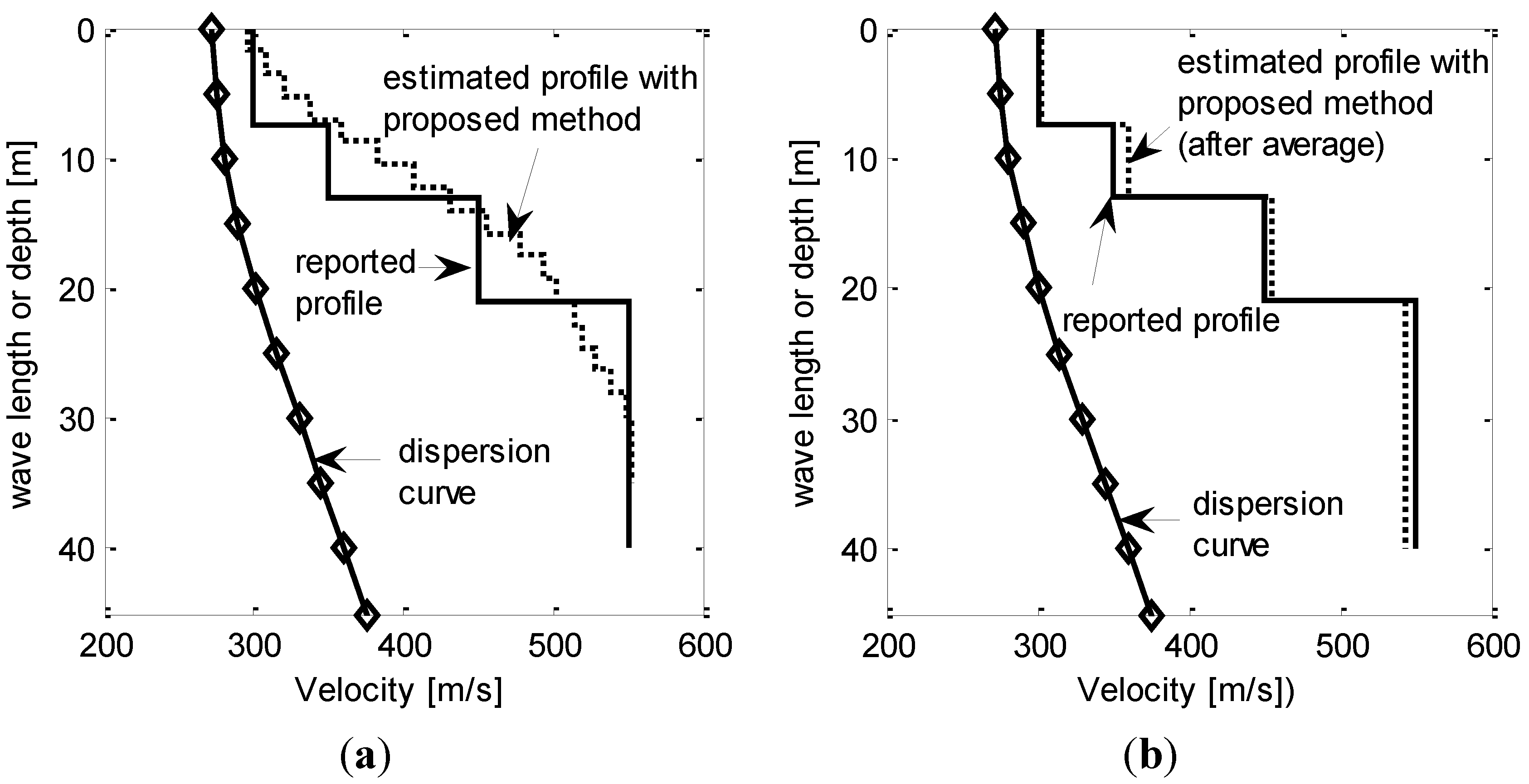
5.2. Ascending Stiffness Profile

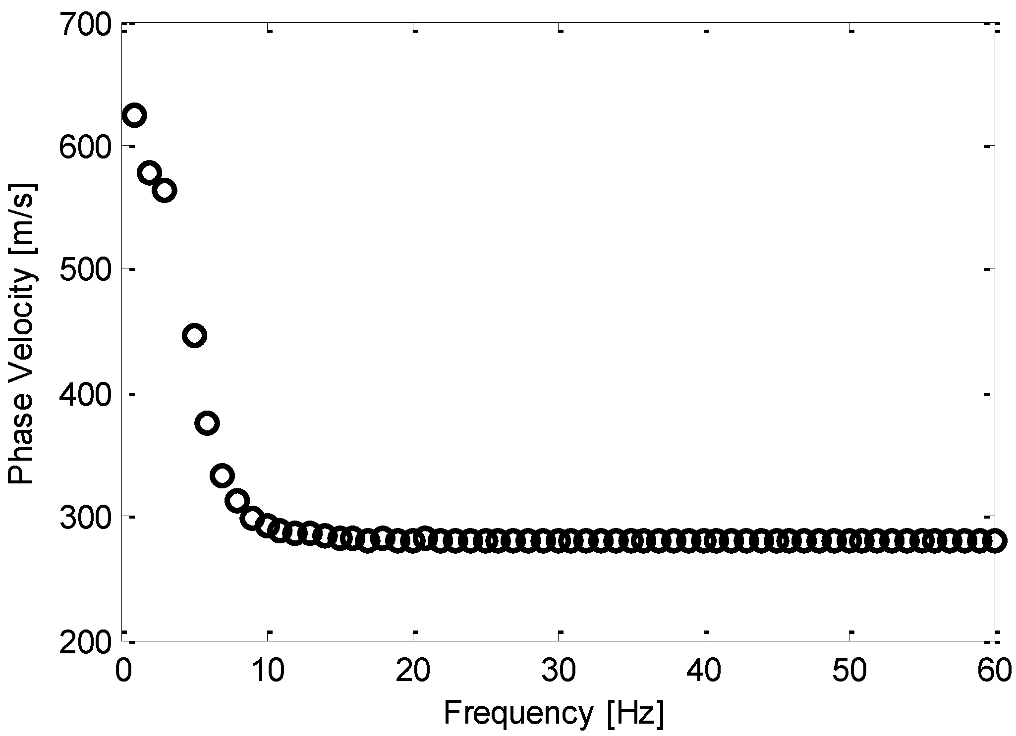
A layered structure with ascending shear velocities along depth is selected to simulate a typical geological site. In this scenario, stiffness of layers increases with depth. Two softer layers are sitting on the harder infinite half-space soil. Table 1 shows the layer configuration and material properties. A forward simulation program based on stiffness matrix method is developed to analyze the wave propagation. The calculated dispersion curve is compared with the result by Zomorodian et al. [18], who used the same profile configurations. Figure 8 shows the forward simulation of dispersion curve by stiffness matrix method. It can be verified via the dispersion curve in Figure 8 using the program developed by the authors, which matches with the dominant fundamental mode of the published curve in Figure 6a by Zomorodian et al., exactly. Thus, the calculated dispersion curve in this paper is trustable.

Table 1. Layered structure with ascending velocity profile.

Layers	Thickness	Damping Ratio	Poisson’s Ratio	Unit Weight	Shear Velocity	Elastic Modulus
1	20 m	0.005	0.35	20 kN/m3	300 m/s	495 MPa
2	20 m	0.005	0.35	20 kN/m3	500 m/s	1376 MPa
3	infinite	0.005	0.35	20 kN/m3	700 m/s	2698 MPa

Table 1. Layered structure with ascending velocity profile.

Layers	Thickness	Damping Ratio	Poisson’s Ratio	Unit Weight	Shear Velocity	Elastic Modulus
1	20 m	0.005	0.35	20 kN/m3	300 m/s	495 MPa
2	20 m	0.005	0.35	20 kN/m3	500 m/s	1376 MPa
3	infinite	0.005	0.35	20 kN/m3	700 m/s	2698 MPa

Figure 8. Analytical dispersion curve (dominant mode).

Figure 8. Analytical dispersion curve (dominant mode).

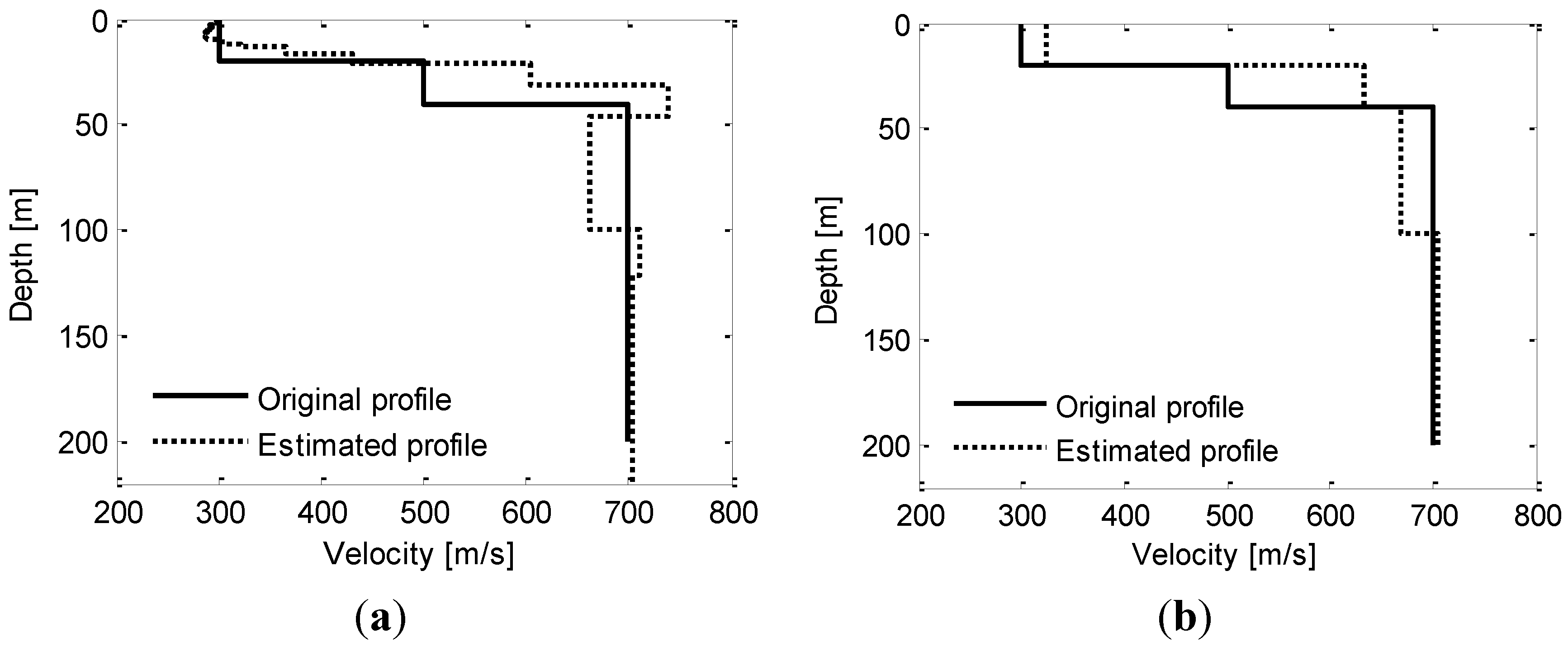
Figure 9. Inverted shear velocity profile vs. original profile for ascending stiffness profile; (a) Inverted shear profile; and (b) Averaged shear profile.

Figure 9. Inverted shear velocity profile vs. original profile for ascending stiffness profile; (a) Inverted shear profile; and (b) Averaged shear profile.

Based on the analytical dispersion curve by stiffness matrix method, the shear velocity profile is estimated using the proposed fast inversion algorithm. The inversion calculation is finished extremely quickly in less than one second. The results are compared with the given profile in Figure 9. It can be seen from the Figure 9a that the inverted shear velocity profile follows the overall trend of the original profile and matches the value best at the top layer and infinite layer. It is also shown from the figure that the inverted layer depths are not the same as the original because the inversion method automatically takes the data points at dispersion curve as thin layers by discretization. Better comparison is made by averaging the inverted shear velocity profile in the same depths of the original profile, as shown in Figure 9b. It can be seen from the averaged comparison that results for the top and infinite layer have the best accuracy and the middle layer has lower accuracy.

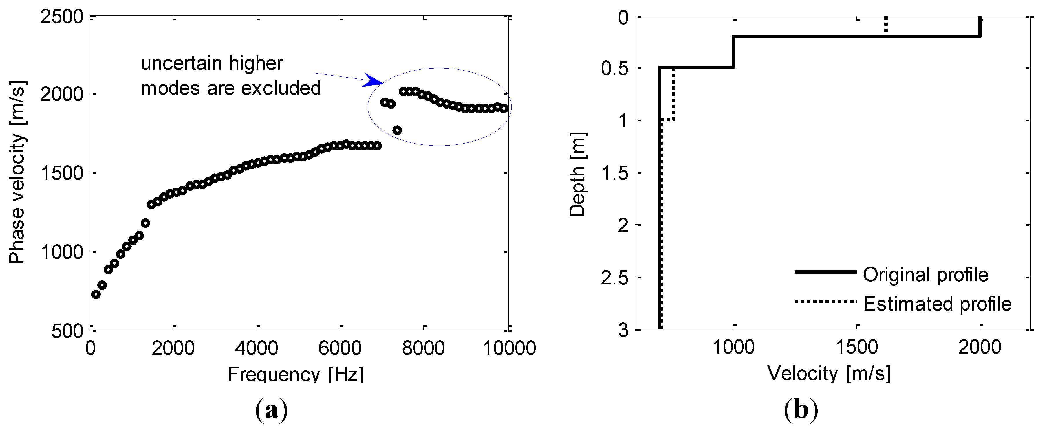
5.3. Descending Stiffness Profile and Limitations

A layered structure with descending shear velocities along depths is selected to simulate the typical pavement structure. Two harder layers are sitting on the softer infinite half-space soil. Table 2 shows the layer configuration and material properties.

Table 2. Layered structure with descending velocity profile.

Layers	Thickness	Damping Ratio	Poisson’s Ratio	Unit Weight	Shear Velocity	Elastic Modulus
1	0.2 m	0.005	0.35	20 kN/m3	2000 m/s	22025 MPa
2	0.3 m	0.005	0.35	20 kN/m3	1000 m/s	5506 MPa
3	infinite	0.005	0.35	20 kN/m3	700 m/s	2698 MPa

Table 2. Layered structure with descending velocity profile.

Layers	Thickness	Damping Ratio	Poisson’s Ratio	Unit Weight	Shear Velocity	Elastic Modulus
1	0.2 m	0.005	0.35	20 kN/m3	2000 m/s	22025 MPa
2	0.3 m	0.005	0.35	20 kN/m3	1000 m/s	5506 MPa
3	infinite	0.005	0.35	20 kN/m3	700 m/s	2698 MPa

Figure 10 shows the calculated analytical dispersion curve and inverted shear velocity profile, in comparison with the original profile in same depths. Due to the multi-mode reflection in the top layers, the higher modes were extracted in the dispersion analysis. Since the proposed inversion is based on the assumption that fundamental mode is apparent and dominant with homogeneous half-space or ascending stiffness profile; thus, the phase velocity at higher modes need to be excluded before the inversion analysis to avoid misleading. After the excluding of the dominant higher modes, the comparison in the Figure 10b shows that the inverted shear velocity profile approximates the original profile except the top layer.

Figure 10. Inverted shear velocity profile vs. original profile for descending stiffness profile; (a) Analytical dispersion curve; and (b) Inverted averaged shear profile.

Figure 10. Inverted shear velocity profile vs. original profile for descending stiffness profile; (a) Analytical dispersion curve; and (b) Inverted averaged shear profile.

6. Comparison with Other Methods

In order to further compare the efficiency of the proposed fast inversion method, a few solved problems are selected from other literature and re-analyzed. The reported dispersion curves in these examples are selected as the input to the inversion analysis with the new method proposed in this paper. It is found that the proposed inversion algorithm gives very similar estimations with the results of all tested examples. Two representative examples and comparisons are presented below to illustrate the accuracy of the proposed inversion algorithm.

6.1. Example 1

The first example is selected from the research report by Nazarian et al. [7]. A geological field was tested with the SASW method. The dispersion curve was generated according to phase difference between two geophones. The inversion process was based on the iterative guess-and-check strategy with forward analytical analysis. Dunkin’s extension of Haskell-Thomas’s approach [29] was used as the forward analytical approach.

The dispersion curve in Figure 11 is measured from the report [7] and used as the dispersion curve input of the proposed inversion algorithm. The new estimated shear velocity profile is also plotted in Figure 11 in comparison with the reported estimation. It can be seen in Figure 11a that the automatically generated shear velocity profile has more detail layer classifications. In order to better compare with the reported result, the estimated profile is averaged according to the same depth as the report, as shown in Figure 11b. According to Figure 11b, the estimated profile and reported profile are close to each other.

Figure 11. Estimated shear velocity profiles using the proposed inversion algorithm; (a) Automatically generated shear velocity profile; and (b) Averaged shear velocity profile. (The vertical axis scale is the wavelength for the dispersion curve and depth for profile).

Figure 11. Estimated shear velocity profiles using the proposed inversion algorithm; (a) Automatically generated shear velocity profile; and (b) Averaged shear velocity profile. (The vertical axis scale is the wavelength for the dispersion curve and depth for profile).

6.2. Example 2

The second example is selected from the Ph. D dissertation by Joh [8]. In this dissertation, a global inversion and an array inversion strategy were utilized to enhance the inversion efficiency. The SASW experiment was performed at the site behind a fire station on Treasure Island. The inversed velocities were compared with the results determined by cross-hole measurement and OYO * (GEO Instruments Corporation in Japan, Kawaguchi, Japan) suspension logging in the dissertation as Figure 6.10 (pp. 171), Figure 6.13 (pp. 176), and Figure 6.12 (pp. 175) by Joh [8].

Based on the same dispersion curve, the shear velocity profile is estimated with the inversion method of the present work. The estimated profile is plotted in Figure 12 in comparison with the results reported in Joh’s dissertation. It can be seen from Figure 12 that both the reported and estimated profiles go around the positions of cross-hole and OYO suspension logging. Larger differences are also found in the deeper depths between reported and estimated profile, as well as between the measured results of OYO suspension logging. This shows the results of the proposed inversion method has similar accuracy with the method applied in Joh’s dissertation.

Figure 12. Estimated shear velocity profiles in comparison with the reported result by Joh [8]. (The vertical axis scale is the wavelength for the dispersion curve and depth for profile).

Figure 12. Estimated shear velocity profiles in comparison with the reported result by Joh [8]. (The vertical axis scale is the wavelength for the dispersion curve and depth for profile).

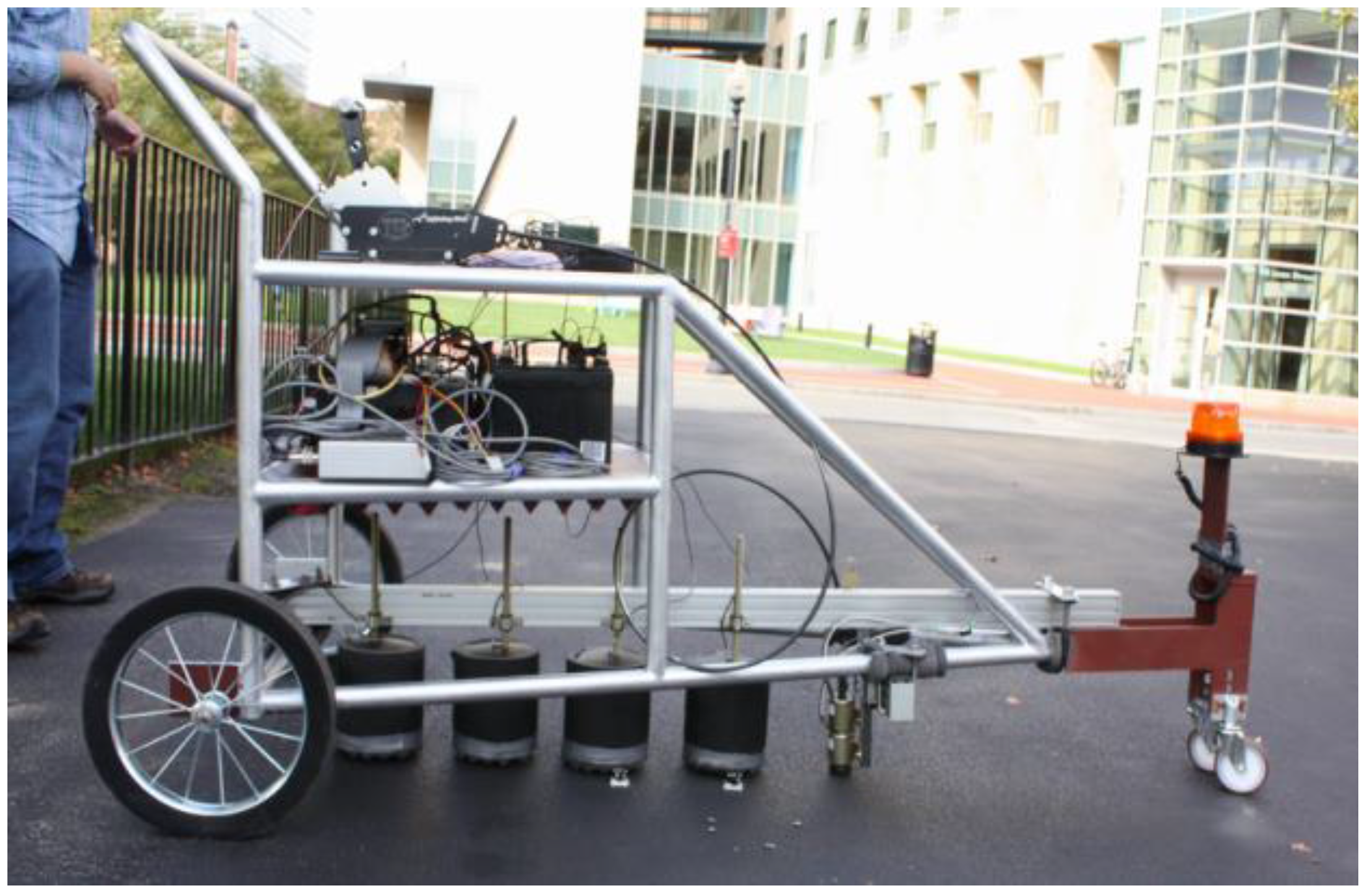
7. Field Test with Fast Inversion Algorithm

A Mobile Acoustic Subsurface Sensing (MASS) system is developed using the air-coupled SASW technique and proposed fast inversion algorithm [30]. Mobile tests are performed using the developed MASS hardware and software system at an asphalt parking lot of Northeastern University. Test locations are marked by chalk stick with 60 cm apart. The microphone array is 1 cm above the ground in 20 cm spacing. The cart moves along the chalk marks and the hammer impacts at the marked points. Five impacts are applied at each location. Sampling rate is set to 200 kHz for all sensors. The entire system is handled by one person, including pushing the cart and operating the test control. Figure 13 shows the test system and test site.

Figure 13. Mobile testing at Northeastern University Campus.

Figure 13. Mobile testing at Northeastern University Campus.

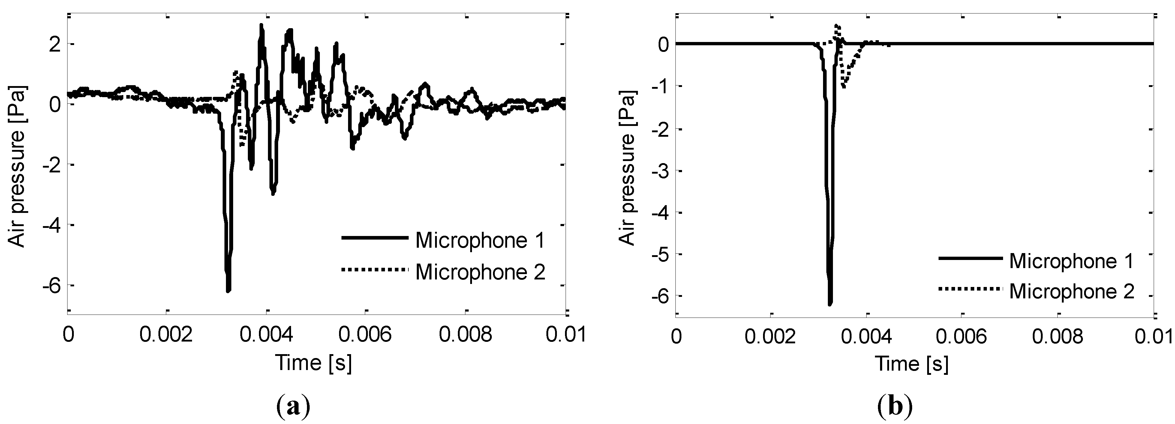
Figure 14 shows the time history of a hammer impact at the parking lot. The acoustic wave radiated by surface waves in the two microphones 40 cm apart are extracted by applying a Hanning window on the raw data. The window size of the first channel is decided to be the double of the time length of the minimum peak value. The window size of the second channel is the size of the first channel plus the travel time of hammer noise between two channels in acoustic speed. It can be observed from the Figure 14b that the extracted radiating surface wave is fairly smooth and representing its features appropriately.

Figure 14. Microphone data of parking lot test: (a) Raw acoustic data; and (b) Filtered radiating surface wave.

Figure 14. Microphone data of parking lot test: (a) Raw acoustic data; and (b) Filtered radiating surface wave.

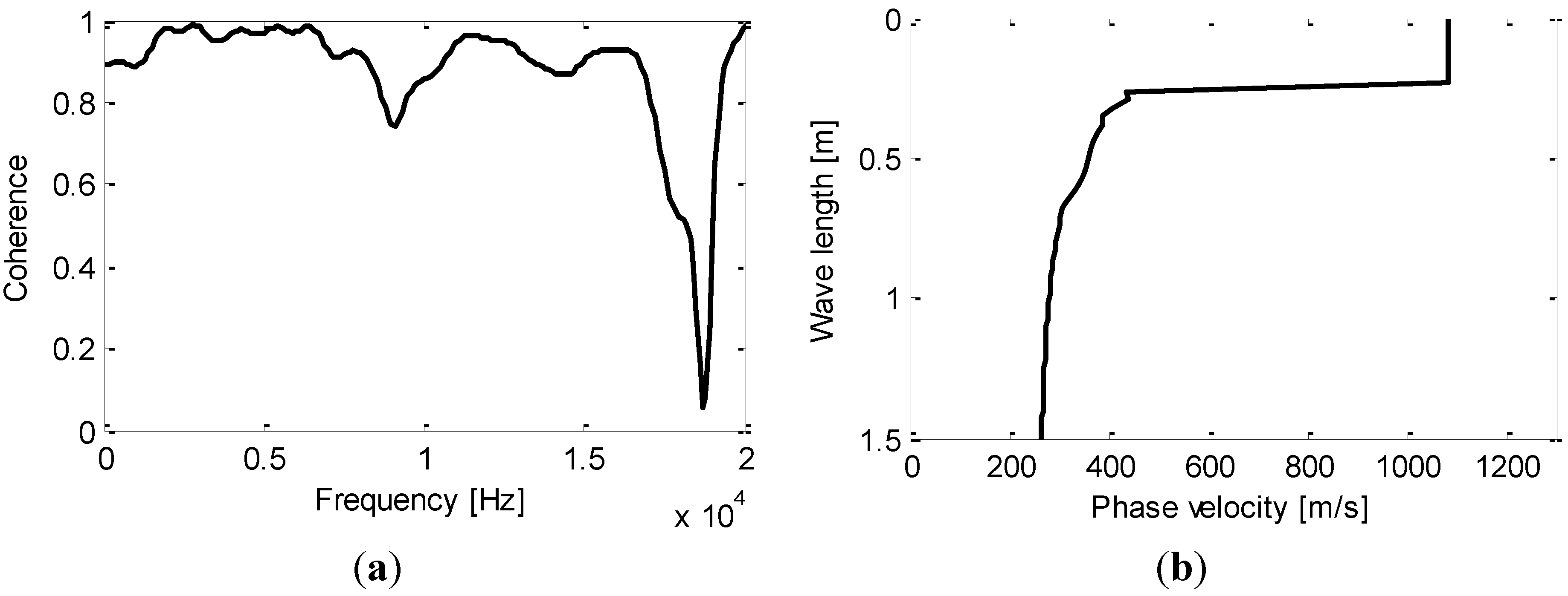
Figure 15 shows the coherence and dispersion curve between two microphone channels. It can be seen from Figure 15a that good coherence could be above 0.9 up to 8000 Hz. The effective dispersion curve is calculated for this frequency band and plotted in Figure 15b. In order to realize the inversion algorithm robustly, the dispersion curve has to start from the surface (as zero depth). Thus, the phase velocity at the unidentified shallower depth (frequency above 8000 Hz) is assumed to be the same as the first identified depth. This assumption can be seen from abrupt vertical segment at the top of the dispersion curve in Figure 15b.

Figure 15. (a) Coherence function; and (b) Dispersion curve.

Figure 15. (a) Coherence function; and (b) Dispersion curve.

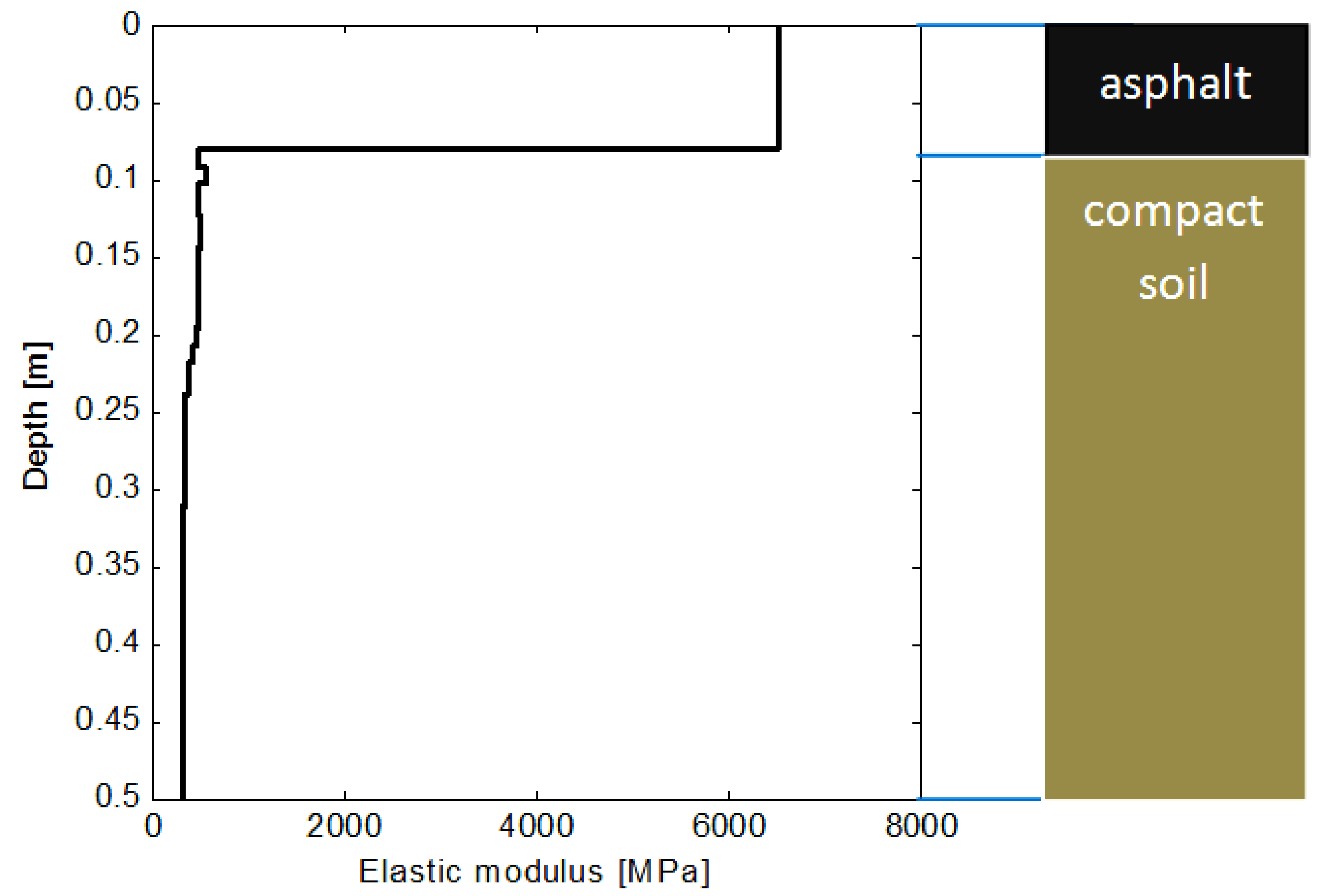
The final estimated profile of elastic modulus is presented in Figure 16. Mass density of 1800 kg/m³ and Poisson’s ratio of 0.3 as standard values for asphalt were used in the calculation of the elastic modulus. According to the profile, the first asphalt layer has an estimated depth of 0.08 m and estimated elastic modulus of 6500 MPa, which falls into the range of a regular asphalt concrete material from 4400 MPa to 6800 MPa. However, comparing the estimated value, 324 MPa, at the depth of 0.4 m with the range of 65–130 MPa for regular compact soil, estimation accuracy is not as good at this depth in this test due to the fine discretization of thin layers. However, the elastic modulus curve approaches to the standard range for compact soil as the general trend. With the benefits of fast analysis in field tests, the proposed algorithm still demonstrates efficient inversion capability.

Figure 16. Estimated elastic modulus profile at parking lot test.

Figure 16. Estimated elastic modulus profile at parking lot test.

8. Conclusions and Future Work

The Spectral Analysis of Surface Wave (SASW) is a widely practiced method for subsurface profiling in geological studies, as well as civil engineering. The air-coupled SASW is a promising extension for fast non-contact inspection. So far, these methods are largely limited as a point-to-point stationary test due to the low efficiency test procedure and inversion algorithm. A fast inversion algorithm is proposed in this paper based on the fundamental relationship between particle velocity, shear velocity and phase velocity of surface wave. The phase velocity is expressed as the weighted combination of the shear velocities of subsurface layers within penetrated depth by the surface wave with a certain wavelength. An iterative procedure is then established to invert the shear velocity profile from the measured dispersion curve. The accuracy of this inversion procedure is validated using the analytical dispersion curve for given layered structures through the stiffness matrix method. It is also illustrated through two examples in comparison with the results reported by other researchers. Since the proposed inversion algorithm is purely algebraic expressions and therefore extremely fast, it offers more opportunities for the air-coupled SASW method to be advanced as a fast or even real-time inspection method in the future.

Several limitations are noticed when applying the proposed algorithm. The proposed weighted combination relationship between shear velocity profile and phase velocity is based on the fundamental mode of the surface wave. Only the fundamental mode of the complete dispersion curve is applied in calculation. For scenarios where stiffness ascends with depth, such as geological sites, the proposed inversion would work well. For the scenarios where the impact response of the ground is dominated by multiple mode vibrations due to stiffer overlays above a softer base and sub-grade materials, such as highway pavement, higher mode responses are dominating. In this case, advanced techniques are needed to extract the fundamental mode dispersion curve in order for this algorithm to be applied appropriately. The candidates for these pre-processing methods include the Gabor filter. The other solution is the help of Lamb wave inversion to handle the dominant higher modes for stiff top layers. In future work these efforts need to be embedded as a kind of pre-processing algorithm in real-time.