Soil Moisture Mapping in an Arid Area Using a Land Unit Area (LUA) Sampling Approach and Geostatistical Interpolation Techniques

Abstract

Soil moisture (SM) plays a key role in many environmental processes and has a high spatial and temporal variability. Collecting sample SM data through field surveys (e.g., for validation of remote sensing-derived products) can be very expensive and time consuming if a study area is large, and producing accurate SM maps from the sample point data is a difficult task as well. In this study, geospatial processing techniques are used to combine several geo-environmental layers relevant to SM (soil, geology, rainfall, land cover, etc.) into a land unit area (LUA) map, which delineates regions with relatively homogeneous geological/geomorphological, land use/land cover, and climate characteristics. This LUA map is used to guide the collection of sample SM data in the field, and the field data is finally spatially interpolated to create a wall-to-wall map of SM in the study area (Garmsar, Iran). The main goal of this research is to create a SM map in an arid area, using a land unit area (LUA) approach to obtain the most appropriate sample locations for collecting SM field data. Several environmental GIS layers, which have an impact on SM, were combined to generate a LUA map, and then field surveying was done in each class of the LUA map. A SM map was produced based on LUA, remote sensing data indexes, and spatial interpolation of the field survey sample data. The several interpolation methods (inverse distance weighting, kriging, and co-kriging) were evaluated for generating SM maps from the sample data. The produced maps were compared to each other and validated using ground truth data. The results show that the LUA approach is a reasonable method to create the homogenous field to introduce a representative sample for field soil surveying. The geostatistical SM map achieved adequate accuracy; however, trend analysis and distribution of the soil sample point locations within the LUA types should be further investigated to achieve even better results. Co-kriging produced the most accurate SM map of the study area.

1. Introduction

Soil moisture (SM) has a significant impact on environmental processes and water resource management. However, it is often difficult to get an understanding of SM spatial variability due to the lack of ground truth SM data. Mapping SM spatial variability has been a topic of active research for the past two decades, and geographical information systems (GIS), geostatistical techniques, and remote sensing data can deliver important information for estimating and mapping SM [1,2,3,4,5]. Although the remote sensing technology has been providing much information about SM at various spatial scales/spatial resolutions, there often still remain unobserved areas (e.g., due to cloud cover), and remote sensing data also needs to be validated by ground truth data or existing maps. Field measurement undoubtedly gives the most accurate information on SM, but choosing appropriate sample locations for field measurements can be challenging [1,2]. In the previous work involving SM mapping from field samples, some researchers have compared different sampling densities/sampling designs [2], while others have focused on comparing different spatial interpolation techniques [1,2,3,4,5,6,7,8,9,10,11]. However, SM mapping studies typically do not consider, from the beginning to the end the entire process, generating a map of homogeneous areas for guiding the selection of field sampling sites, field SM measurement, and finally SM mapping using spatial interpolation techniques. One of the biggest challenges in SM mapping is the soil spatial variability. SM spatial variability is governed by various environmental factors (e.g., soil properties, topography, radiation, precipitation, vegetation, land use) [11,12]. SM variation is also affected by the complex interaction of environmental factors over times, which lead to high temporal variability in SM, in addition to the high spatial variability. An understanding of SM spatial variability across heterogeneous land surfaces has been considered as critical for eco-hydrological research and for vegetation restoration in arid and semi-arid areas [12,13,14]. Soil sampling design and the locations of samples points are very important, and is one of the other challenges in SM studies. Consequently, for overcoming these two major challenges, geospatial databases in GIS and spatial interpolation techniques are powerful tools. Whereas precise field soil sampling is an essential step to obtain accurate SM measurements [15,16,17], GIS provides a variety of useful tools for geo-environmental monitoring, mapping and evaluation, and spatial analysis to explore the spatial relationships between physical phenomena such as soil type, geology, and land cover to help the produce land unit area (LUA) maps [18,19,20,21,22]. LUA is a fundamental concept of ecology, and is defined as an ecologically homogeneous area of land, considering the scale at issue [23]. Consequently, the land unit concept is widely used for land sustainability, land use management, and planning. [24,25,26,27]. In land unit classification, the soil data are as important as geology, landform, climate, and vegetation.

The geospatial database provides the common data access and management framework for ArcMap [24,25,26,27]. The geospatial analysis offers insight about the environments and reveals management options. In the past years, some researchers have been trying to use GIS for soil mapping, especially in soil nutrition and SM by using the geospatial data and interpolation methods [2,28].

In this research, we applied GIS tools for advanced analysis of geospatial data for creating the LUA map as a homogenous field area to guide soil sampling [29,30]. Soil samples should be taken in areas with various physical characteristics (e.g., climate, topography, geology, vegetation, and soil types, etc.). By identifying areas with similar physical characteristics (i.e., LUA types), we can ensure that each of these homogeneous areas is included in the field sampling (and that none are excluded). In other words, the LUA map provides a basis for mapping and transferring landscape knowledge, via evaluation, to application [31,32]. The LUA, made in ArcMap using a geospatial database, has an important role supporting the field soil sampling toward the SM mapping. This LUA can systematically design a homogeneous area which it is easy to take the soil samples in the field, using a global positioning system (GPS), from each polygon randomly.

Using sample points to generate accurate SM maps is quite difficult. Spatial data and spatial interpolation methods play a significant role in environmental dynamic monitoring and mapping. Continuously, toward the SM mapping from sample points, a geostatistical interpolation method has the ability in spatial interpolation for this approach. In past studies, geostatistical techniques were the most popular method to characterize the spatial patterns of SM and the relation to controlling factors [5,33]. A number of research has used the varied spatial interpolation method (over 32 spatial interpolation methods) for environmental modeling and monitoring. Many factors affected in spatial interpolation methods and there are a number of papers in this approach and made a comparison between those methods [2,5,9,25,33,34]. The kriging, co-kriging, and Inverse distance weighting (IDW) are the most frequent methods which are used for spatial interpolation [2,34]. Therefore, these were compared to SM interpolation based on the field sample data.

The main contribution of this paper is its introduction of the land unit area (LUA) approach for SM field sampling, combined with its comparison of different interpolation methods in an arid study area. The LUA map was derived from various geospatial layers, which were combined to delineate areas with homogenous soil, land use/land cover, and climate characteristics. The benefit of the LUA approach is that it considers many of the variables which affect SM spatial variability.

2. Materials and Methods

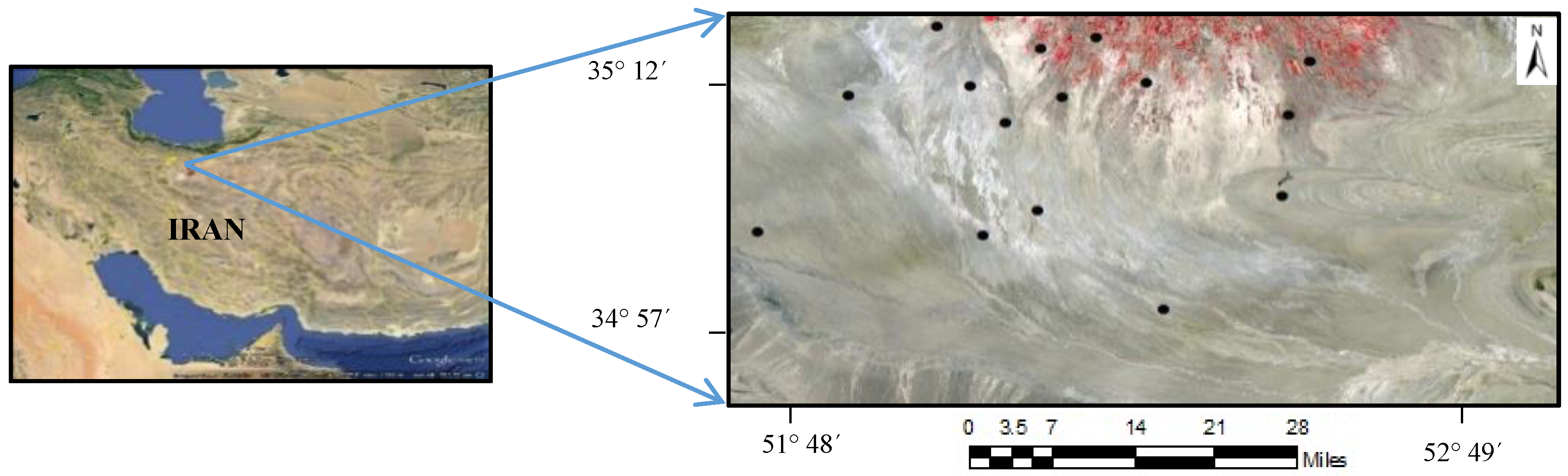
2.1. Study Area

The study area is located in the northern part of Iran (Figure 1). The climate type of the study area is arid and semi-arid (Garmsar, Iran), and the average annual precipitation is 120 mm. Land use in this area is mainly range, wildlife, recreation, agricultural, and unused land, while most land cover in the study area is bare land and sparsely vegetated land, with some cropland in the northern part of the area. Although the climate type in this area is dry, in some parts of the lowland area in the south, the groundwater table is high and near the top soil surface, which causes the soil to be relatively moist. Arid soils do not particularly have a great variety in soil texture, but in the study area, typically, soil is developed in the south-to-north direction, which is caused by an alluvial fan. The significant north-to-south variation in geophysical properties in this study area was the reason it was chosen as the study area for this research.

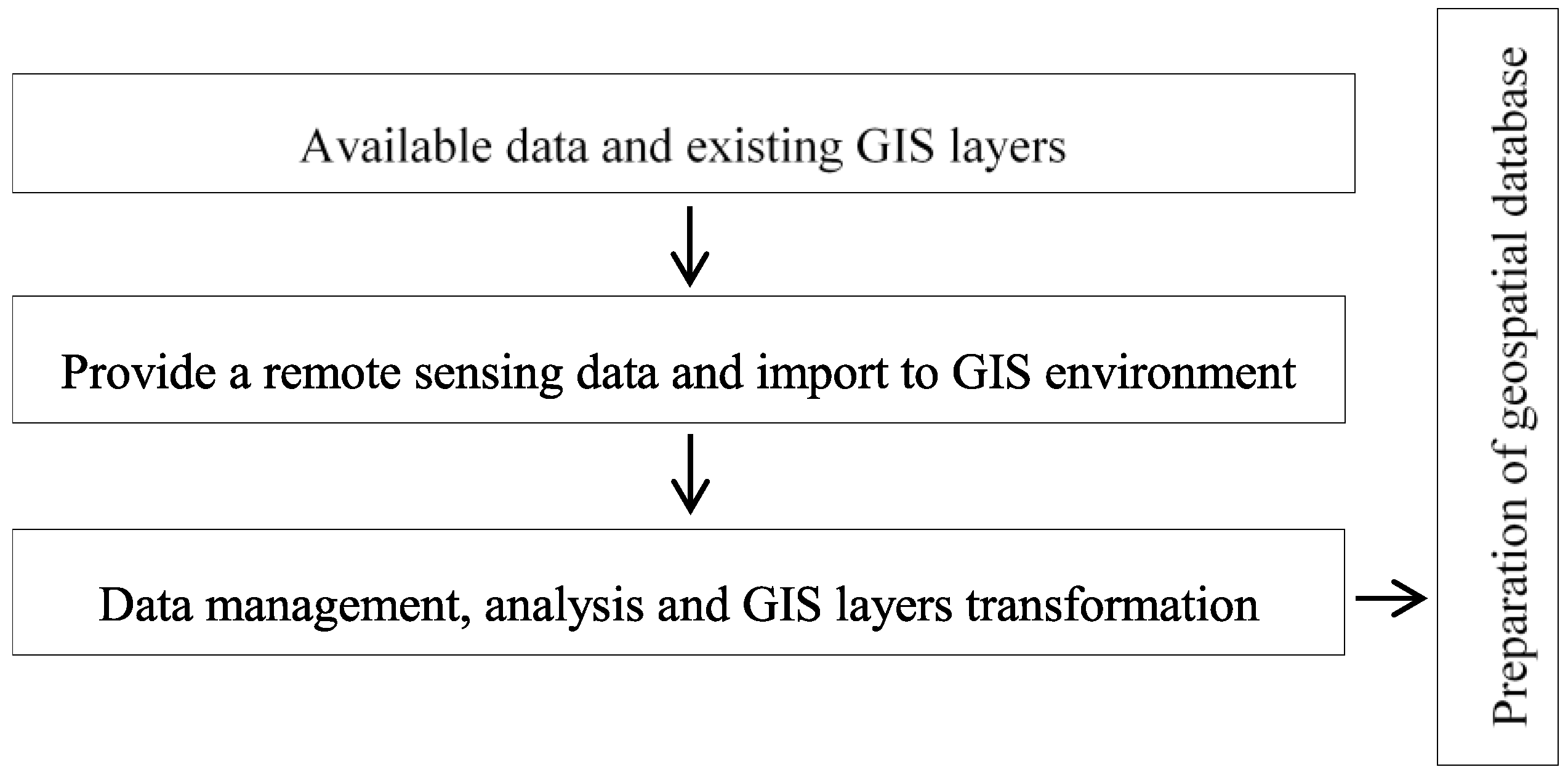
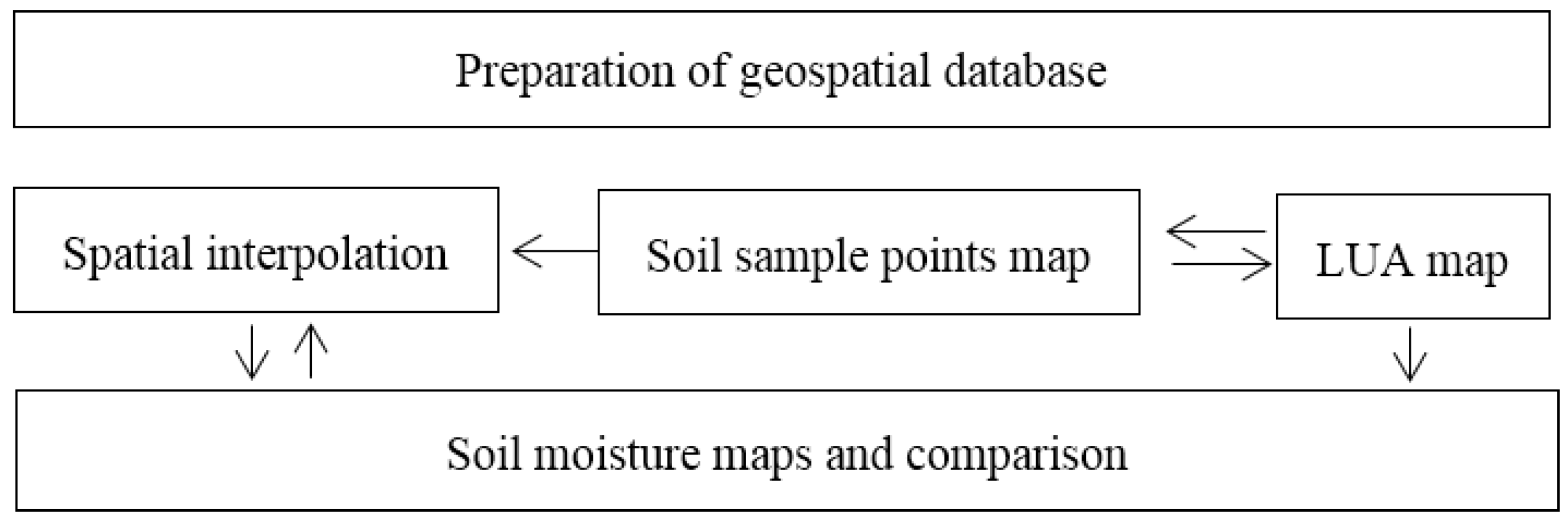
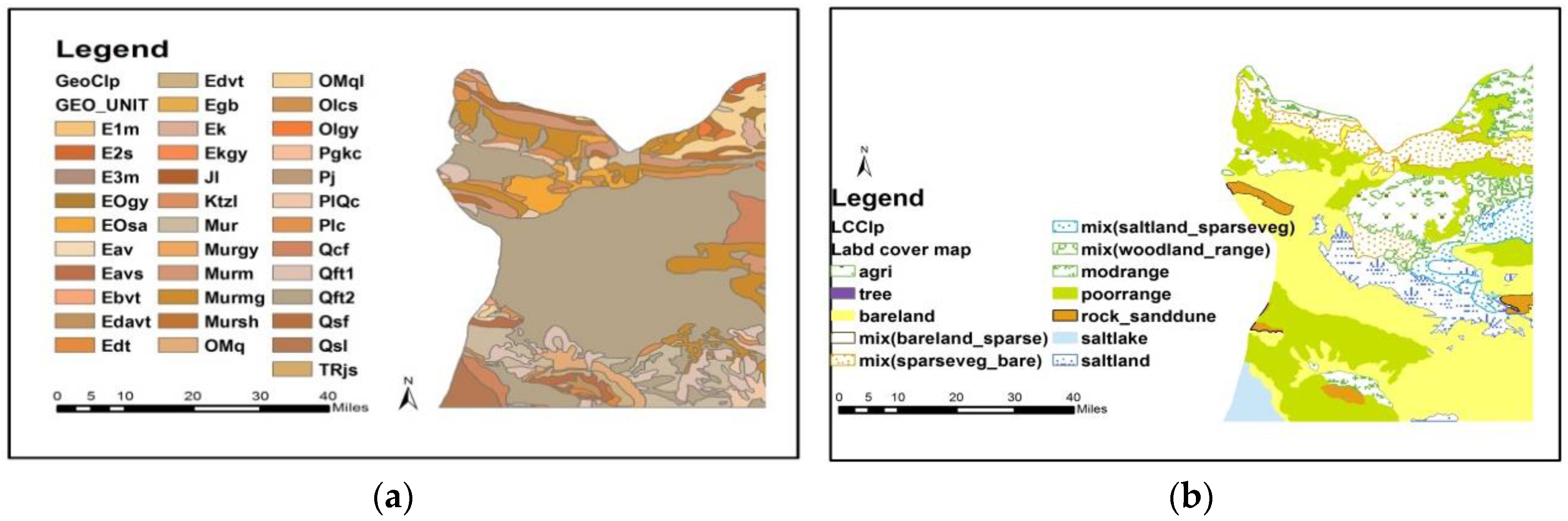
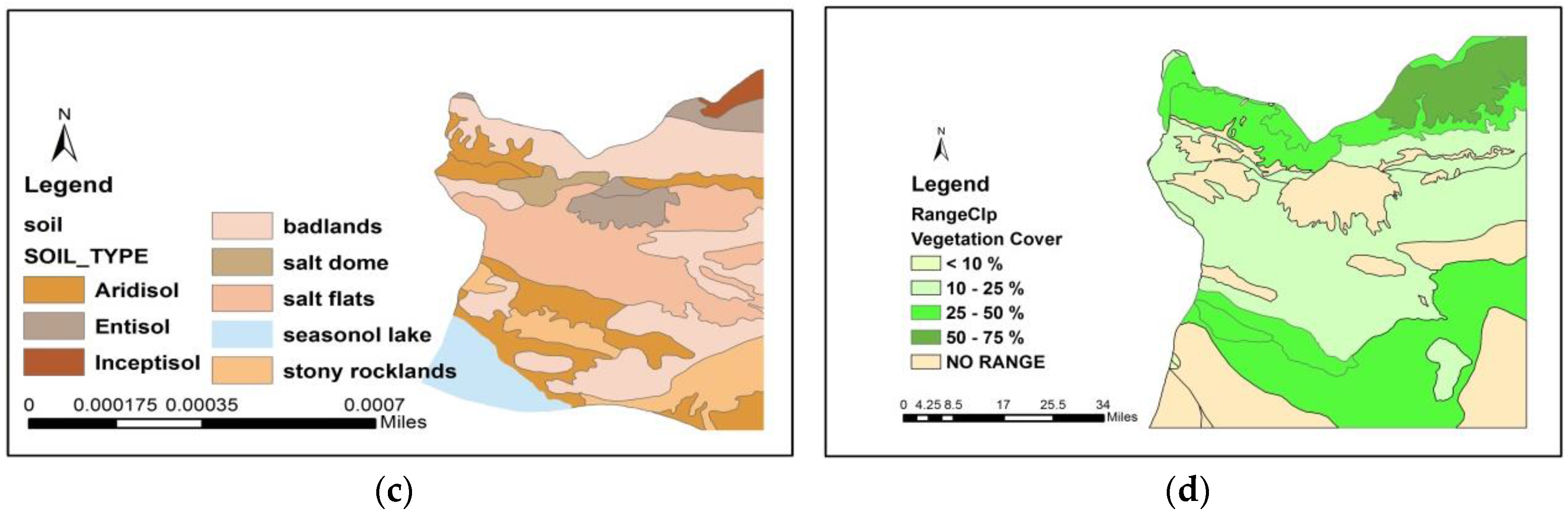
2.2. Preparation of the Geospatial Database

In this study, to generate a geospatial database, firstly we collected the existing data both in digital format and hard copy maps of Semnan province, which covers our study area. This existing data was collected from local reports, unpublished studies, and local organizations. These datasets were created by different surveyors and using different tools, so they were all scanned (if hard copy), georegistered, and projected to a single projection/coordinate system to ensure their compatibility with one another. The Figure 2 has shown the overall work steps of this section. Specifically, the used data were as follows:

• Land cover/use map of Semnan province, produced by Landsat ETM⁺ and TM by Semnan Agriculture Research Organization
• Geological map at a scale of 1:100,000, which was produced in 2010 by Geological Surveying Organization (This map is created in hard copy and digital format based on the aerial photography, geological interpretation, and field work checking)
• The 90 m Digital Elevation Model (DEM)
• Climate data such as precipitation, temperature, and evapotranspiration which was produced by the Meteorological Organization of Semnan province
• Vegetation cover percentage which was produced by the Forest, Rangeland and Watershed Organization
• Soil types and soil regime layers, which were created by the Soil and Water Conservation Institute
• Provide the remote sensing data layers (i.e., water, soil, and vegetation indexes)

The components of the geospatial database, which from the structure out of GIS are included as data input, data storage and management, data analysis and transformation, and data output and presentation. Firstly, we searched for available data and then, provide remote sensing data, such as land cover, geology, vegetation cover, as required for the geospatial database. Data analysis and transformation means the achievement of transformation needed to remove errors from data or to update the data. On the other hand, the data manipulation and analysis functions determine the information that could be generated and extracted from GIS layers (climate type, soil type, geology, etc.). The result is a geospatial database in the form of maps and tables of attribute values.

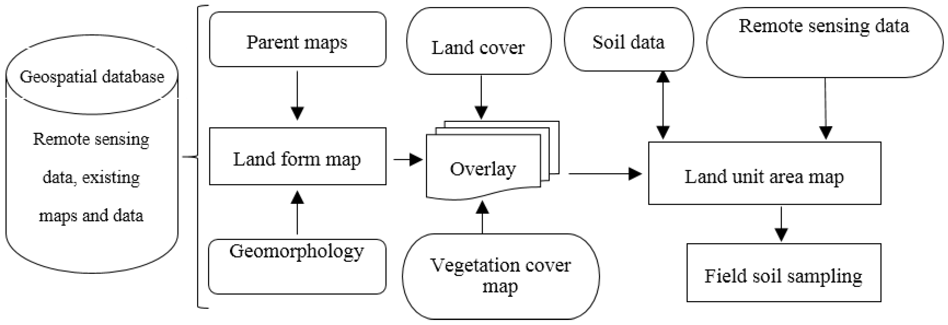
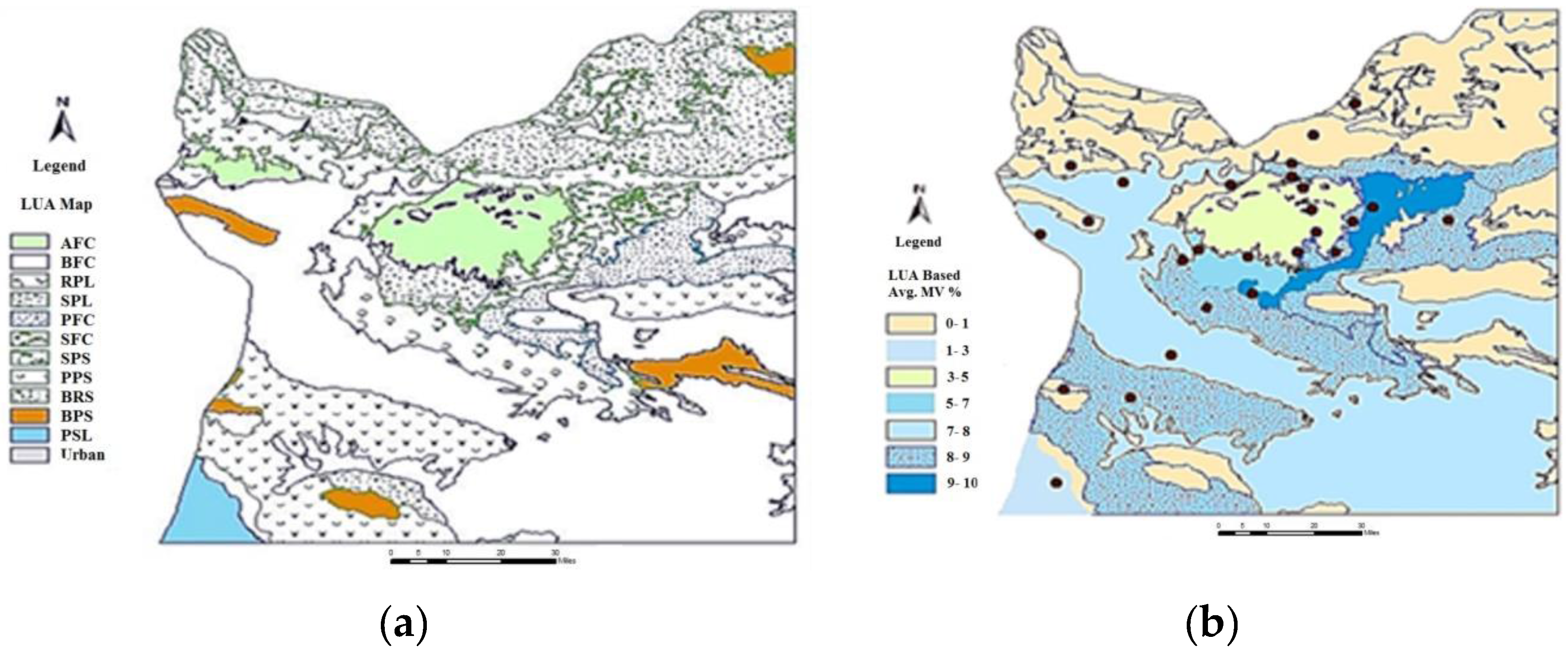
2.3. Derivation of the LUA Map

Research related to land unit areas has typically been limited to ecological studies, such as biodiversity, as this term originated in the ecological sciences [23,24,25,26,27]. We found only one previous study which used the LUA concept for soil research, but it did not consider SM [30]. The previous study suggested a method for soil study using LUA, and their approach was based on a geological and parental material view, while our method is different that it focuses on SM derivation and includes more particular environmental GIS layers which cover environmental factors that influence SM.

The study of SM needs the analysis of various parameters, e.g., physical, climatic, and geo-biological parameters. In this research, for producing homogeneous geo-physical areas (i.e., LUAs) for acquiring soil samples, the following environmental parameters were considered (after the pre-processing of the relevant datasets, as described in Section 2.2):

(1)

Geology

(2)

Soil information (types, regime)

(3)

DEM (topography, slope, curvature)

(4)

Land cover/land use

(5)

Vegetation cover

(6)

DEM (topography, slope, curvature)

(7)

Geomorphology

(8)

Climate data (rainfall, temperature, evapotranspiration)

(9)

Remote sensing information (NDMI and land surface temperature)

(10)

Landform

According to the above GIS layers, we should specify that the soil types and the soil regime data contain different information (

Table 1. Example of physical properties and SM measurement in study area.

Field No.	Soil Texture	Sand %	Silt %	Clay %	SM Vol.%	Land Cover
14	Loam	32.2	49.1	18.7	3.3	Sparse vegetation
11	Silt Loam	20.2	65.2	14.6	6.6	Bare land
13	clay	10.1	33.3	56.6	8.6	Bare land
12	Silt clay	9	52	39.1	5.2	Sparse vegetation
10	Loam	24.2	58.1	17.7	9.5	Bare land

). Landform was derived based on topography, and the land was classified into terrain types on the basis of two morphometric indices: slope and curvature [8,30,32].

The GIS work flow for deriving the LUA map is divided into three phases, and was mainly done in a GIS environment (ESRI ArcGIS 10.1, Chiba University license). The workflow consisted of three phases.

Phase one:

• Reclassification and standardization of the production remote sensing data (land cover/use)
• Production of the base maps (climate, vegetation, lithology)
• Import to the GIS environment
• Create the landform map using geomorphology map and DEM (slope and curvature)
• Overlaying the parent maps, geomorphology, and vegetation cover to create the landform
• Producing the remote sensing data layers (i.e., surface temperature, moisture index)
• Evaluation and addition of the soil data (soil types, soil regime)
• Creation of the geospatial database in GIS to produce the land unit area (LUA) map
• Produced the remote sensing data of Landsat ETM⁺ (13 September 2013) (e.g., NDMI and surface temperature)

Phase two:

• Visual interpretation and validation of the LUA map by remote sensing data layers
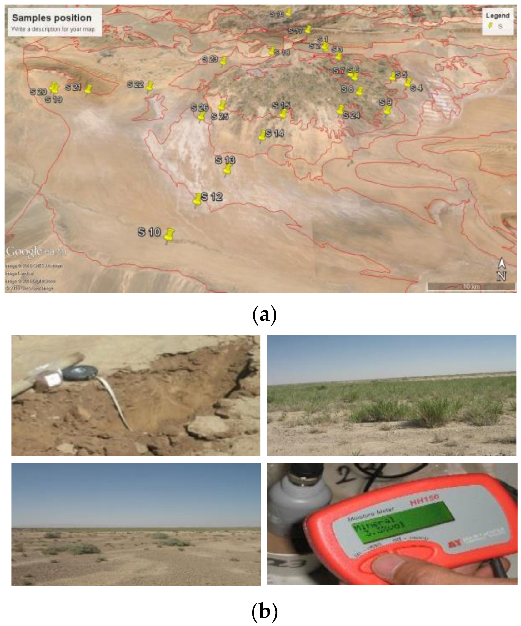
• Using the LUA map as the final guidance map for field soil sampling
• Measuring the SM points in each LUA polygon by TDR

Phase three:

• Creating the SM map using sample points of field and LUA map in GIS
• Using the geostatistical interpolation method in GIS to generate the SM map
• Evaluation and comparison of SM maps of LUA, geostatistical, and NDMI

Several types of spatial analysis (e.g., filtering, merging, and overlaying) were performed to produce the LUA map. For example, the landform map was created using the slope curvature based on the DEM and combined with the geology map. The land form map, in raster format, was generalized by filtering it using the Majority Filter operator of ArcGIS to reduce the number of unwanted features, such as single pixels or small pixel agglomerates with an area smaller than 150 ha, which is considered to be the minimal mapping unit according to the final scale of the map (1:250,000). In addition, all raster data layers were converted into vector layers, and polygons smaller than a threshold fixed by the operator were eliminated by merging them into the wider joining polygon with the longest shared edge. In the next step, these shape files were thoroughly cleaned up by means of a vector rationalization process and used to derive the landform map. Finally, the landform map was combined with the land cover and vegetation percentage cover map to produce the LUA map. Figure 3 shows the entire work flow for creating the LUA map.

2.4. Field Survey of SM

The first step for field work is the selection of sample locations for collecting the field SM measurements. A composite soil sample should represent a uniform field area that has similar environmental characteristics such as climate, topography, geology, land use, vegetation, and soil type, etc., In field surveying, there are a number of different sampling approaches that can be applied depending on the objectives, and they are strongly influenced by scale. Common sampling designs include; grid sampling, random sampling, random stratified sampling, transects, and target sampling [7]. Therefore, one important step is to define the homogeneous site for each location before sample designing which, in this case, we used the random sampling within each of the LUA map polygons.

In this research based on the limitation of remote sensing data propagation in the soil, we took a sample from the top soil with a target sampling design. The target sampling approaches on the subject define the homogenous area and then took the sample in each LUA polygon. In total, twenty-five samples of soils were collected from different LUAs. At least two samples were collected using Global Positioning System (GPS), using a soil sampling tool kit from each LUA, respectively, at depths of 0–10 cm (top soil). The field work was done during September 2013 in study area (Figure 4).

All at once the SM was measured by TDR (time domain reflectance) from the top soil in the field. Then, 0.5 kg of soil was taken and transported to the laboratory by a plastic tube and analyzed the physical properties and measured the moisture again (Table 1). In fact, in this research soil samples for laboratory experiment were prepared in two steps involving in-field moisture conditions and dried soil conditions after oven drying. After field work, the SM of the soil samples was measured once again by TDR in the laboratory and weighed carefully to record the field moisture condition. These samples were oven-dried in 24 h by 120 °C and then weighed again for calculating the gravimetric SM, and tested the accuracy of the TDR measurement as well.

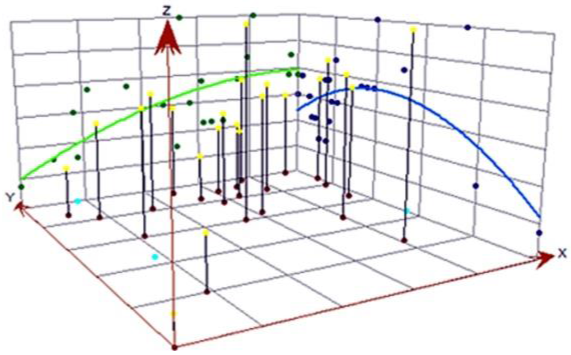
2.5. Spatial Interpolation Methods

Deriving the SM by field points sampling data is another challenge for SM mapping [5,34]. After understanding the general spatial distribution of SM in the field for selecting soil sampling locations, which we suggest using the geospatial data for in the previous sections, the grid surface of SM needs to be produced based on the field measurements. Geostatistics is a branch of statistical theory related to the interpolation and mapping of distributed data. Geostatistical analysis methods are those that are based on statistical models that consider spatial autocorrelation (i.e., the principle that two data points close to each other are more likely to have similar values than two data points located farther apart). The regionalized variable concept is the basis for geostatistic, and states that the spatial variation of any variable might be expressed as the sum of three components [2]:

• A structural component, associated with a constant mean value or a polynomial trend;
• A spatially-correlated random component (auto-correlative component); and
• A white noise or residual error term that is spatially uncorrelated

A recent review article found that, out of the 32 most popular interpolation methods, the inverse distance weighting (IDW), ordinary kriging (OK), and ordinary co-kriging (OCK) methods were the most frequently used in environmental studies [2]. Kriging models estimate the values at unsampled locations by a weighted averaging of nearby samples. The estimation of ordinary kriging is given by;

$$z\left(x\right)={\displaystyle \sum }_{i=1}^{\mathrm{n}}\lambda \underset{¯}{\mathrm{z}}\left(xi\right)$$

(1)

where z(x) is the unknown value needs to be estimated, λ is the weight of the point xi with a given value of z(xi). The correlations among neighboring values are modeled as a function of the geographic distance between the points across the study area, defined by a variogram. Kriging involves a various combination of linear regression and it is the based on a normal regression followed by ordinary kriging. Co-kriging takes advantage of correlation which might be exit among the variable of interest and more measured variables [31]. In general, kriging methods perform better than non-geostatistical methods [2]. Therefore, it has the high potential to apply the point measurements and create the map from field sampled SM data. Some studies showed that co-kriging is superior to kriging [2,7]. In this research, the kriging and co-kriging (ordinary) are applied for SM mapping using sample points' measurements.

In the IDW method, the weightings are solely a function of the distance between the point of interest and the sampling points for i = 1, 2, …, n. Considering the distance d_i between these two points, the value of a point of interest point takes the form:

$$z={\displaystyle \sum }_{i=1}^{\mathrm{n}}\frac{{\mathrm{z}}_{\mathrm{i}}/{\mathrm{d}}_{\mathrm{i}}²}{{{\displaystyle \sum }}_{i=1}^{n}1/{\mathrm{d}}_{\mathrm{i}}²}$$

(2)

where Z is the interpolated value of the point of interest; Z_i is the value of sampling point i (i = 1, …, n); d_i is the distance between the interpolated and sampled values. A robust interpolation method is needed to do this, and many have been discussed significantly in the literature. Among numerous interpolation methods, there is no report which obviously mentioned a method is uniquely optimal for interpolation; therefore, the best interpolation method for a specific condition can only be obtained by comparing their results to each other [1,5,29]. Some research has been done on comparing different interpolation methods in a variety of situations. However, there have been few reports comparing different interpolation methods for SM. In this research, we used the twenty-five sample points based on LUA and axillary data of soil and vegetation cover percentage map for co-kriging.

2.6. Creation of SM Maps

The final step in this research produced the SM map in the arid area by sample points using the spatial interpolation method based on the geostatistical method in GIS which is presented in the last section. After preparation of the SM data from each point in field surveying the point map created in ArcMap and then the geostatistical tools was applied on the point map. The three soil maps produced by kriging, co-kriging, and IDW method and these maps were compared to each other by RMSE and QQ plot. The Figure 5 has shown the overall flowchart for producing the SM map.

The other SM map was created based on the LUA map in ArcMap. In this map, each polygon of LUA map gave the value of the SM sample and created the grid-based SM. Moreover, the SM map of Landsat remote sensing incorporates multi-band indexes, such as NDMI.

3. Results and Discussion

3.1. Geospatial Database to Produce the LUA Map

As mentioned before, the tools of remote sensing and GIS are important to achieve the results of this study; therefore, satellite images are used to produce the data, such as land cover, moisture and vegetation indices, etc. GIS techniques were used to composite, extract, and analyze data and create the derived information related to geo-environmental indexes in the form of SM.

Table 2. A frame of the attribute table of soil type and soil regime map in the geospatial database.

ID	Soil Regime	Soil Type
239	Lithic Calciustepts, Coarse to Medium, Typic Calciustepts, Fluventic, Haploxerepts, Undulating	Inceptisol
603	Rock Outcrops—Litihic Xerorthents—Typic Haploxerepts, Hilly	Entisol
824	Typic, Torriorfhents, coarse to medium, Typic, Haplogypsids, Typic, Haplogypsids, Gentiy, Undulatir	Entisol
1105	Typic, Haplogypsids, Coarse to Medium, Typic, Torriorfhents, Typic, Haplocalcids, Gently, Undulate	Aridisol
1106	Typic, Haplogypsids, Coarse to Medium, Typic, Torriorfhents, Typic, Haplocalcids, Gently, Undulate	Aridisol
1355	Xeric, Haplosalids, medium, Xeric ,Torrifluvents, Typic, Aquisalids, level	Aridisol

has shown the example of the attribute table of soil information in the geospatial database. All of the geospatial analysis, standardizing of the layers, has been done in ArcMap software. Figure 6 has shown some input maps as base layers in a geospatial database.

3.2. Land Unit Area (LUA) Map Production

Several geospatial techniques were used in a GIS environment to produce the LUA map (Figure 7). In ArcMap we used the overlaying by weighting, meaning we obtained the score in the range of 1–5 points for each environmental layer that was more influenced by SM. This score was decided based on the field observation and the basic terminology of SM relationships in the study area. The score of each layer is as follow: the landform, 5; the vegetation cover, 4; and the land cover types, 3. This map is solved by expert interpretation, field observation, a comparative visual check by Google Earth, and remote sensing data. This point map is ready for field work as a soil surveying base map. The LUA map includes 11 classes with unique codes related to their general characteristics, as shown in

Table 3. Unit code descriptions of the land unit area map (Figure 7).

ID	Info
AFC	Agriculture with mixed cropland, alluvial, and colluvial parent material, deep soil, loam to clay soil texture
BFC	Bare land in plain, alluvial fan, clay soil and silt soil, fine to coarse sandstone, lowland
RPL	Rangeland, plain, soil with good depth and fertilizing, clay loam, and clay
SPL	Sparse vegetation and mix with crop and follow, plain land with loam and clay soil texture
PFC	Smooth plain, fine texture soil with salinity and limitation for drainage, limitation for plants, halophyte plants
SFC	Rangeland mix by shrubland, alluvial fan with high ground water table with limitation for farming, coarse to fine soil
SPS	Sparse vegetation in rangeland, plain, halophyte plant in winter, little soil saline, loam to clay texture
PPS	Poor range, plain, soil salinity limitation, sandy soil, soil erosion
BRS	Bare land in rocky mountain, sandstone with undeveloped coarse soil
BPS	Badlands with soil with physical and chemical limitation for plants
PSL	Plain area, temporal salt lake

. During the field work and observation, we understood the LUA polygons could reasonably cover the spatial variability of geophysical parameters which affected SM, to detect the best areas for introducing representative soil samples. The largest LUA unit was BFC in the middle part of the study area, and the smallest was RPL in the south. In the study area, usually in southern and northern parts the LUA, units are smaller in size than in the middle part due to the low variability in a land geophysical characteristic, such as land cover, geology, and soil in the middle part of the study area. It seems, in an arid environment, due to lower variability in other geo-biological factors, such as soil and vegetation type, the land cover can be counted as one of the most important base layers for generating the LUA map.

In addition to the SM maps we produced by spatial interpolation of the field sample data. We also produced another SM map for visualization purposes (to show the different SMs of each LUA type) by assigning the average SM values of a LUA type (obtained from the field sampling) to the corresponding LUA polygons, as shown in Figure 7b. The comparison of this map with NDMI and the geostatistical SM map has shown it has a more geometric correlation with land surface characteristics.

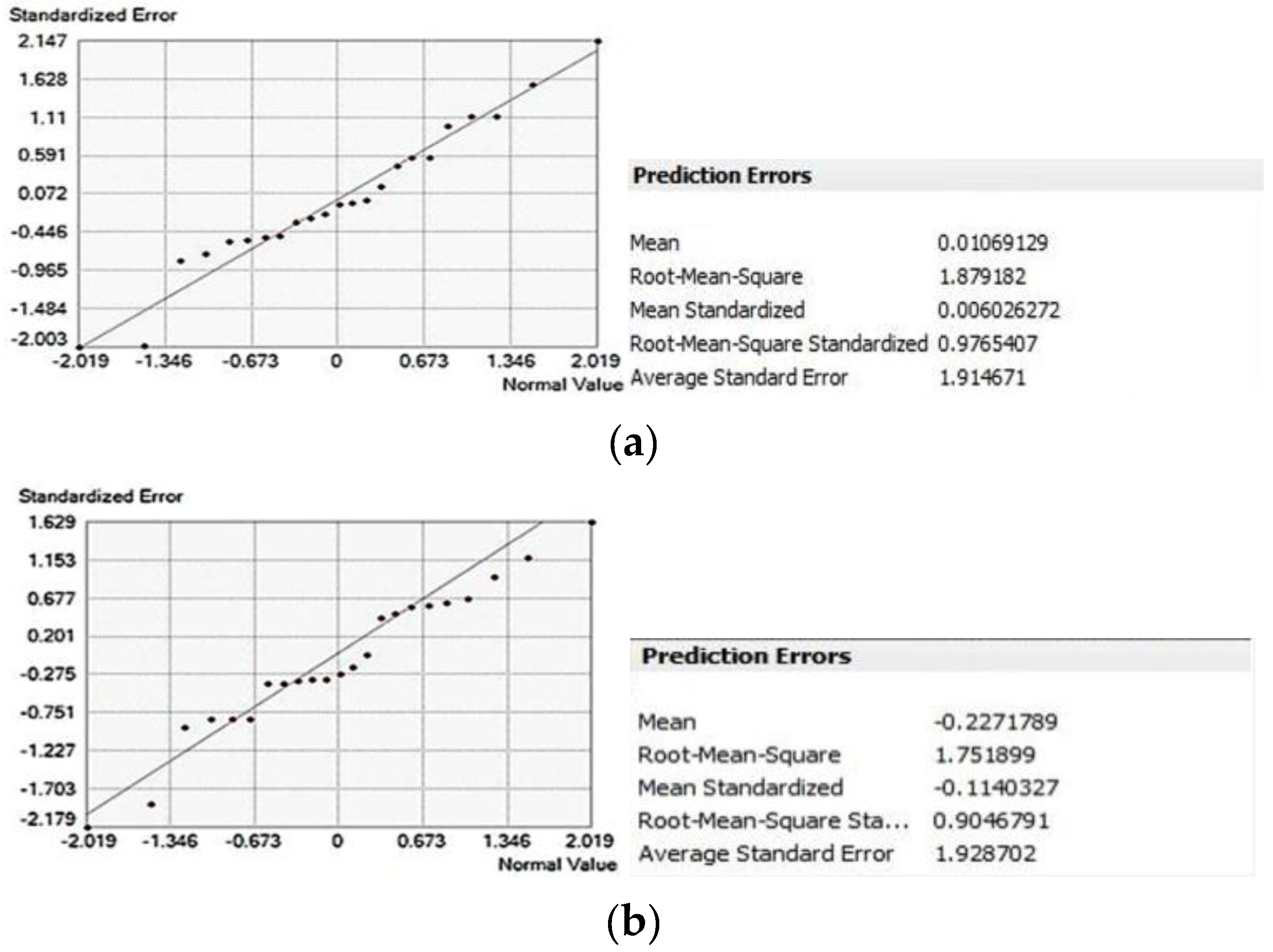
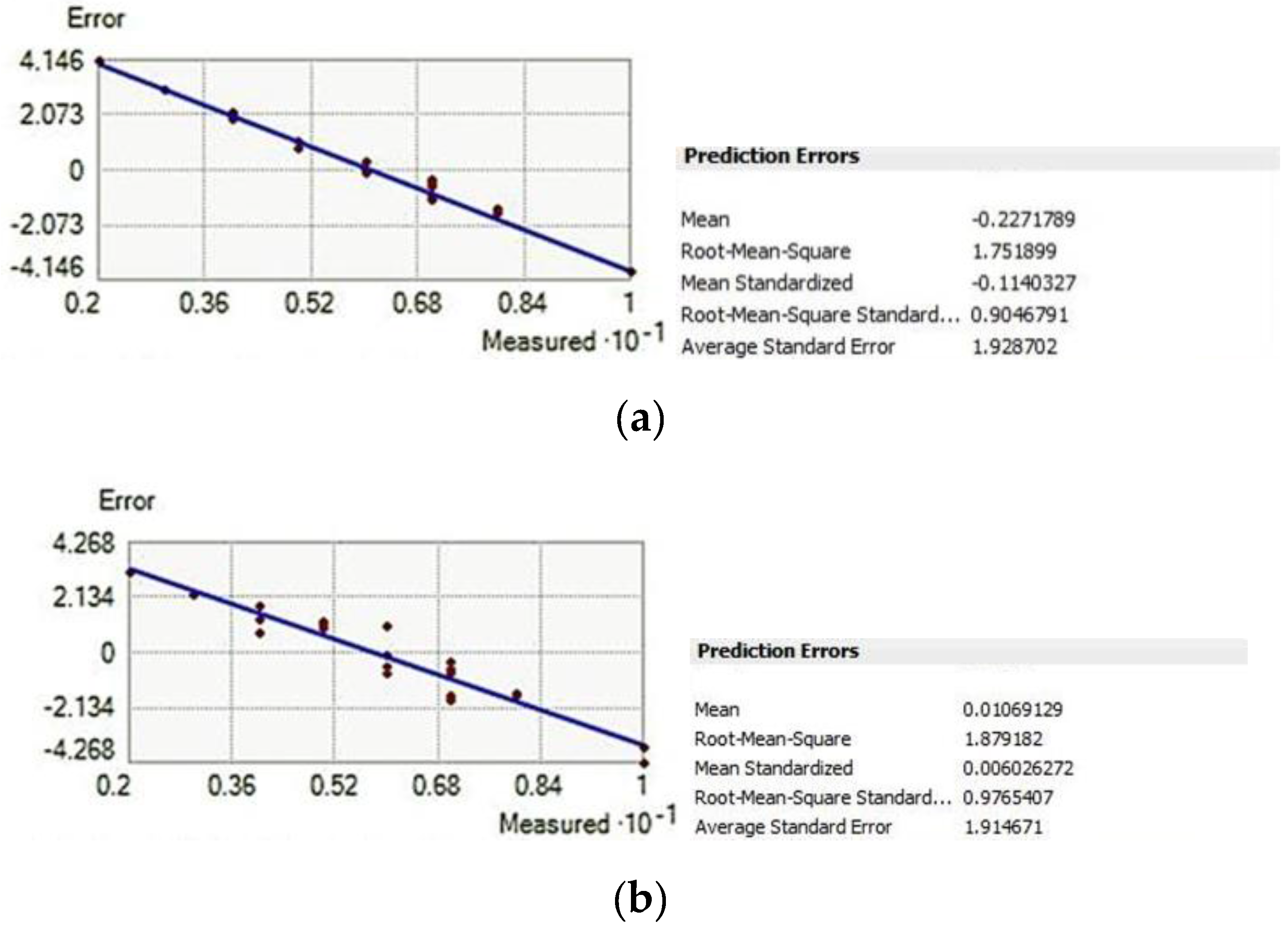
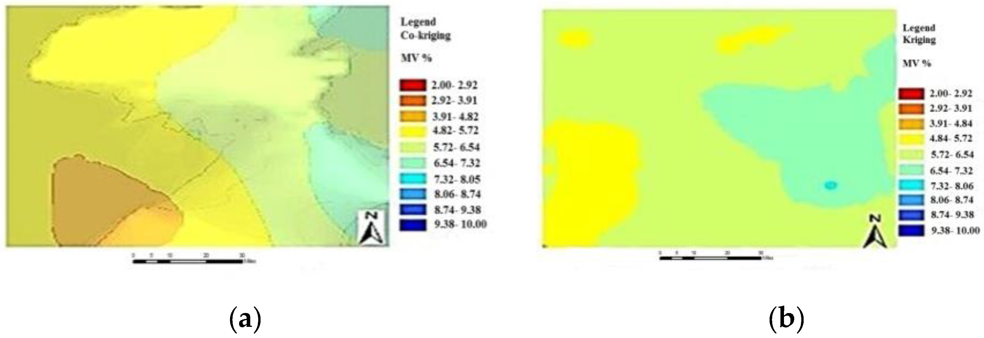
3.3. SM Mapping Using the Spatial Interpolation Method and Comparison

The variogram describes the degree of similarity between attribute values at sample sites x and x₊h as a function of their geographical separation or lag h. In variograms, the distance between data points (X-axis) is plotted against the semivariance (Y-axis) (Figure 8a). The covariance map of prediction map has shown in Figure 8b.

The trend analysis was done in the study area using point project attribute data of SM samples (Figure 9). Figure 9 shows the trend in spatial variation of SM. The trend results have shown that the green trend line with values at the end of Y axis has a gradual reducing trend, and then it has an increasing trend in the X-axis. However, the blue trend line from the furthest end of the X-axis in the Y-axis shows a gradual reduction. Rendering to two above curves, order to trend removal was interpolated such that spatial variations in the northeast-to-southwest direction were intensive, but there is a gradual variation in the direction of northwest-to-southeast.

Co-kriging uses information on several variable types. The key variable of concern is Z₁, and both autocorrelation for Z₁ and cross-correlations between Z₁ and all other variable types are used to make enhanced predictions. It is appealing to use information from other variables to help make predictions, but one depends on the other. Co-kriging requires more estimation, including estimating the autocorrelation for each variable, as well as all cross-correlations. Theoretically, it is no worse than kriging because if there is no cross-correlation you can simply rely on autocorrelation for Z₁. For co-kriging, we used the soil map and vegetation canopy percentages as additional explanatory variables. The empirical variogram was produced by using the three different maps, SM points from field surveying, soil map, and vegetation cover map. LUA map was linked to SM point map as an as a basic map of it. The sill, range and nugget were investigated by these three variables of soil, vegetation, and LUA against the points of the sample. In fact, the sill, nugget, and range are approving the variable which has enough correlation with sample points. Since the study area was not very wide and the LUA map was very helpful to detect the polygons for sampling, the range, sill, and nugget have shown a logical trend among them. The range value shows that the sample has an acceptable distribution of distance within the LUAs.

Kriging collects the interpolation methods that rely on semi-variogram models of spatial autocorrelation to generate predicted values and other information regarding the distribution of values for each location in the study area through quintiles and probability maps, or via geostatistical simulation, which provides a set of possible values for each location. The data distribution and model results can be visualized in the normal QQ plot, in which the standard normal distribution is plotted on the x-axis (Figure 10). If the data is normally distributed, the points will be located along the 45-degree reference line.

Validation is possible by comparing two methods by cross-validation, but instead of using the same dataset to build and evaluate the model, two datasets are used; one to build the model and the other as an independent test of performance. In this research, we used the Subset Features tool to randomly split the data into training and testing subsets. For validation, we are comparing which method is best for our dataset. The first we compared between the two different technique of kriging and co-kriging and then with IDW (Figure 10 and Figure 11). The comparison is based on the root mean square error (RMSE), standardized mean error, and average standard error. Normally, the best model is the one that has the standardized mean close to zero, the smallest root mean squared prediction error, the average standard error nearest the RMS prediction error, and the standardized RMS prediction error nearest to one. In our comparison, the co-kriging method achieved the lowest RMSE and standardized mean, so it was recognized as the best model (Figure 10b), followed by kriging and, finally, IDW (Figure 11).

Finally, after the analysis of the interpolation method, the SM map was derived by the geostatistical technique of ordinary kriging, co-kriging, and IDW in ArcGIS software (Figure 12a–c). The normalized different moisture index (NDMI: TM4-TM5/TM4+TM5) was produced by Landsat TM data for comparing the result visually (Figure 12d). These three maps have shown the moisture in the range of 2–10 percentages, which the kriging method of the study area shows in the moderate range, and IDW shows all ranges in the legend in this variable range of moisture. Normally, in the study area, the moisture content is increasing from north to south, as shown in the maps; there are some areas which are covered by wet soil due to the geomorphology of the plains (Playa), which led to high level groundwater. Although the groundwater level is high, on the other hand, evaporation is high as well; therefore, the salt plain appeared. In this way, the spatial interpolation method is very significant to understand the trend of the prediction map using a point sample with regional distribution variability. Therefore, according to this variability, regionalized variable theory is used to model the spatial dependence of soil properties by variogram analysis, which is required for spatial prediction.

As we mentioned before, the geospatial database, and the resulting LUA maps, could be useful for field work in soil moisture surveying. In this way, the understanding of interacting with soil, among other environmental factors, would be probable for spatial variability of SM and soil sampling in the field. For achieving the homogenous area as a base map of the field work in soil surveying, the LUA map is the most reliable unit since it comes from different base layers and includes more variables which affect SM properties. Generally, the accessible soil digital map was interpreted using associated and generalized knowledge concerning the impact of topography, geology, and land cover on soil properties. However, the LUA approach for delineating homogeneous areas in terms of soil, geological, vegetation, geomorphology, landform, and land cover is most practicable. Therefore, it seems this study’s method offers a quick and fruitful technique based on the land unit map by using the geospatial database in a GIS software environment. As a result, this research created a new technique for landscape setup to create the land unit area (LUA) map. For large study areas, much time is needed for soil surveying to understand the spatial distribution of soil properties like SM; therefore, the use of LUA maps to intelligently select soil field sample points is very important.

4. Conclusions

Soil samples in the field must return the overall or average soil characteristics of a homogenous field. For this reason, the new LUA was applied to introduce homogeneous areas for selecting soil sample positions in the field. It was found that the technique to produce the land unit area (LUA) from geospatial databases of environmental parameters was effective for the selection of soil sampling and, finally, for SM mapping. The results showed that the LUA map was successful for taking representative sample points of SM. In addition, by updating either make an automatic algorithm in GIS, the changes of any layers in the geodatabase over time and space can be used to update the LUA map for future field work.

Comparison of the four SM maps; three of the geostatistical methods and one based on LUA; the co-kriging method could derive the most accurate SM map, followed by kriging and, finally, IDW. Although it seems the co-kriging could be more flexible than kriging because it makes it possible to add some other explanatory variables for interpolation. For instance, in SM mapping, it is possible to add the variable of either soil geology or other information which we have in our disposal. Finally, the most important factor for creating a reliable model in geostatistical spatial interpolation is a dataset with a satisfactory spatial distribution of sample points. This means an understanding of soil spatial variability and modeling and mapping is very important to derive the more accurate SM map.

In this study, we have attempted the production of a SM map from soil survey data, taking into account soil spatial variation in the field using GIS-based techniques from the beginning (the soil sampling design) to the end (SM mapping by geostatistical interpolation). Not only has an attempt been made to evaluate or model the generated digital soil maps, this research reflects the complete process of soil sampling, soil spatial variation consideration, and spatial interpolation methods. Further study is recommended on how to better take advantage of geospatial database technology with higher resolution input layers to achieve the more detailed scales of LUA map and accurate result of a SM outputs. Additionally, further study can investigate how the components of the SM interact with one another to impact the environmental factor affected by soil spatial variability, and finally, attempt to automatically create the LUA in GIS.

References

1. Yuanyuan, D.; Yong, W. Research on the spatial interpolation methods of SM based on GIS. In Proceedings of the International Conference on Information Science and Technology, Nanjing, China, 26–28 March 2011; pp. 26–28.
2. Jin, S.; Andrew, D.H. A review of comparative spatial interpolation method in environmental sciences: Performance and impact factor. J. Ecol. Inform. 2010, 6, 228–241. [Google Scholar]
3. Tomislav, H.; Gerard, B.M.H.; David, G.R. About regression-Kriging: From equation to case studies. Comput. Geosci. 2007, 33, 1301–1315. [Google Scholar]
4. Wei, S.; Budiman, M.; Alex, M. Analysis and prediction of soil properties using local regression-Kriging. Geoderma 2010, 171–173, 16–23. [Google Scholar]
5. Zhao, P.P.; Shao, M. Soil water spatial distribution in dam farmland on the Loess Plateau, China. Acta Agric. Scand. 2010, 60, 117–125. [Google Scholar] [CrossRef]
6. Takagi, K.; Lin, H.S. Changing controls of soil moisture spatial organization in the Shale Hills Catchment. Geoderma 2012, 173–174, 289–302. [Google Scholar] [CrossRef]
7. Zhu, Q.; Lin, H.S. Comparing ordinary Kriging and regression Kriging for soil properties in contrasting landscapes. Pedosphere 2010, 20, 594–606. [Google Scholar] [CrossRef]
8. Bishop, T.F.A.; McBratney, A.B. A comparison of prediction methods for the creation of field-extent soil property maps. Geoderma 2001, 103, 149–160. [Google Scholar] [CrossRef]
9. Xueling, Y.; Bojie, F.; Yihe, L.; Ruiying, C.; Shuai, W.; Yafeng, W.; Changhong, S. The multi-scale spatial variance of SM in the semi-arid Loess Plateau of China. J. Soils Sediment. 2012, 12, 694–703. [Google Scholar]
10. Rosenbaum, U.; Bogena, H.R.; Herbst, M.; Huisman, J.A.; Peterson, T.J.; Weuthen, A.; Western, A.W.; Vereecken, H. Seasonal and event dynamics of spatial SM patterns at the small catchment scale. Water Resour. Res. 2012, 48. [Google Scholar] [CrossRef]
11. De Benedetto, D.; Castrignanò, A.; Quarto, R. A geostatistical approach to estimate SM as a function of geophysical data and soil attributes. Proced. Environ. Sci. 2013, 19, 436–445. [Google Scholar]
12. Yao, X.; Fu, B.; Lü, Y.; Sun, F.; Wang, S.; Liu, M. Comparison of four spatial interpolation methods for estimating SM in a complex terrain catchment. PLoS ONE 2013, 8, e54660. [Google Scholar]
13. Mohamed, M.Y.; Abdo, B.M. Spatial variability mapping of some soil properties in El-Multagha agricultural project (Sudan) using geographic information systems (GIS) techniques. J. Soil Sci. Environ. Manag. 2011, 2, 58–65. [Google Scholar]
14. Han, X.; Li, X.; Hendricks Franssen, H.J.; Vereecken, H.; Montzka, C. Spatial horizontal correlation characteristics in the land data assimilation of SM. Hydrol. Earth Syst. Sci. 2012, 16, 1349–1363. [Google Scholar] [CrossRef]
15. Marin, P.-G.; Xanat, A.-N.; Jose, A.C.-M.; Martín, A.M.-B. Spatial patterns of soil degradation in Mexico. Afr. J. Agric. Res. 2011, 6, 1109–1113. [Google Scholar]
16. He, Y.; Song, H.Y.; Zhang, S.J.; Fang, H. Study on the spatial variability and the sampling scheme of soil nutrients in the field based on GPS and GIS. In Proceedings of the 27th Annual International Conference of the Engineering in Medicine and Biology Society, Shanghai, China, 1–4 September 2005; pp. 5942–5945.
17. Diana, A.-F.; Marin, P.-G.; Xanat, A.-N. Driving factors for forest fire occurrence in Durango State of Mexico: A geospatial perspective. Chin. Geogr. Sci. 2010, 20, 491–497. [Google Scholar]
18. Goovaerts, P. Geostatistics for Natural Resources Evaluation; Oxford University Press: New York, NY, USA, 1997. [Google Scholar]
19. Grunwald, S.; McSweeney, K.; Lowery, B.; Rooney, D. Continuous description of soil attributes on a landscape in Southern Wisconsin. In Proceedings of the ASA-CSA-SSSA Annual Meeting, Baltimore, MA, USA, 18–22 October 2007.
20. Jacobs, H.M. Practicing land consolidation in a changing world of land use planning. Kart Plan. 2000, 60, 175–182. [Google Scholar]
21. Kevin, J.; Jay, M.; Ver, H.; Konstantin, K.; Neil, L. Using ArcGIS, Geostatistical Analyst. Available online: http://dusk2.geo.orst.edu/gis/geostat_analyst.pdf (accessed on November 2015).
22. Harahsheh, H.; Tateishi, R. Environmental GIS database and desertification mapping of West Asia. In Proceedings of the Workshop of the Asian Region Thematic Programme Network on Desertification Monitoring and Assessment, Tokyo, Japan, 28–30 June 2000.
23. Zonneveld, I.S. The land unit a fundamental concept in landscape ecology, and its applications. Landsc. Ecol. 1989, 3, 67–86. [Google Scholar] [CrossRef]
24. Juergensmeyer, J.C.; Roberts, T.E. Land Use Planning and Development Regulation Law; West Academic Publishing: St Paul, MN, USA, 2013. [Google Scholar]
25. Vacca, A.; Marrone, V.A. The land unit and soil capability map of Sardinia (Italy) at a 1: 50,000 scale: The pilot area of Pula-Capoterra. In 20th World Congress of Soil Science, Vienna, Austria, 27 April–2 May 2014; p. 186.
26. Papadimitriou, F. Modeling landscape complexity for land use management in Rio de Janeiro, Brazil. Land Use Policy 2012, 29, 855–861. [Google Scholar] [CrossRef]
27. Lisio, A.; Russo, F. Thematic maps for land-use planning and policy decisions in the Calaggio stream catchment area. J. Maps. 2010, 6, 68–83. [Google Scholar] [CrossRef]
28. Soil Survey Division Staff. Soil Survey Manual 18; U.S. Department of Agriculture: Washington, DC, USA, 1993.
29. Upchurch, D.R.; Wilding, L.P.; Hartfield, J.L. Methods to evaluate spatial variability. In Reclamation of Disturbed Lands; CRC Press: Boca Raton, FL, USA, 1988; pp. 201–229. [Google Scholar]
30. Vacca, A.; Loddo, S.; Melis, M.T.; Funedda, A.; Puddu, R.; Verona, M.; Fanni, S.; Fantola, F.; Madrau, S.; Marrone, V.A.; et al. A GIS based method for soil mapping in Sardinia, Italy: A geomatic approach. J. Environ. Manag. 2014, 138, 87–96. [Google Scholar] [CrossRef] [PubMed]
31. Wilding, L.P.; Bouma, J.; Boss, D.W. Impact of spatial variability on interpretive modeling. Spec. PublSSSA 1994, 39, 61–75. [Google Scholar]
32. Bi, H.X.; Li, X.Y.; Liu, X.; Guo, M.X.; Li, J. A case study of spatial heterogeneity of SM in the Loess Plateau, western China: A geostatistical approach. Int. J. Sediment Res. 2009, 24, 63–73. [Google Scholar] [CrossRef]
33. Atkinsona, P.M.; Lewisb, P. Geostatistical classification for remote sensing: An introduction. Comput. Geosci. 2000, 26, 361–371. [Google Scholar] [CrossRef]
34. Carter, M.R.; Gregorich, E.G. Soil Sampling and Methods of Analysis; CRC Press: Boca Raton, FL, USA, 1993. [Google Scholar]
Figure 1. Study area using Landsat ETM+ data and some field surveying points.
Ijgi 05 00035 g001
Figure 2. GIS framework for preparation of a geospatial database.
Ijgi 05 00035 g002
Figure 3. The flowchart of GIS frame work for creating the land unit area map.
Ijgi 05 00035 g003
Figure 4. (a) The footprint of the LUA map outlined by a red line and sample points in Google Earth and (b) the landscape of some LUA in the field work and SM measurement by TDR.
Ijgi 05 00035 g004
Figure 5. The main steps of geospatial database creating, LUA map, and spatial interpolation methods in GIS to produce the SM map.
Ijgi 05 00035 g005
Figure 6. Examples of (a) geology map and (b) land cover map; (c) soil map and (d) vegetation cover map.
Ijgi 05 00035 g006aIjgi 05 00035 g006b
Figure 7. The LUA map (a) produced by a geospatial database and (b) the SM map based on LUA and sample point in ArcMap.
Ijgi 05 00035 g007
Figure 8. (a) Semivariogram model and (b) covariance map of Kriging method.
Ijgi 05 00035 g008
Figure 9. The experiment of spatial variation of trend analysis of SM using point project attribute data.
Ijgi 05 00035 g009
Figure 10. The subset of standardized error of QQ plot of the distribution of the dataset which is used for (a) kriging and (b) co-kriging models.
Ijgi 05 00035 g010
Figure 11. Cross-validation of subset between the (a) Co-Kriging and (b) IDW result.
Ijgi 05 00035 g011
Figure 12. The SM map created by (a) co-kriging; (b) kriging; (c) IDW method, and (d) NDMI index using Landsat TM data.
Ijgi 05 00035 g012aIjgi 05 00035 g012b