Article

Watershed Land Cover/Land Use Mapping Using Remote Sensing and Data Mining in Gorganrood, Iran

1
Department of Geography, Ferdowsi University of Mashhad, Mashhad 9177948974, Iran
2
Department of Geography and Regional Research, University of Vienna, A-1010 Vienna, Austria
*
Author to whom correspondence should be addressed.
ISPRS Int. J. Geo-Inf. 2016, 5(5), 57; https://0-doi-org.brum.beds.ac.uk/10.3390/ijgi5050057
Submission received: 12 March 2016 / Revised: 13 April 2016 / Accepted: 22 April 2016 / Published: 28 April 2016
(This article belongs to the Special Issue Advances and Innovations in Land Use/Cover Mapping)

Abstract

:
The Gorganrood watershed (GW) is experiencing considerable environmental change in the form of natural hazards and erosion, as well as deforestation, cultivation and development activities. As a result of this, different types of Land Cover/Land Use (LCLU) change are taking place on an intensive level in the area. This research study investigates the LCLU conditions upstream of this watershed for the years 1972, 1986, 2000 and 2014, using Landsat MSS, TM, ETM+ and OLI/TIRS images. LCLU maps for 1972, 1986, and 2000 were produced using pixel-based classification methods. For the 2014 LCLU map, Geographic Object-Based Image Analysis (GEOBIA) in combination with the data-mining capabilities of Gini and J48 machine-learning algorithms were used. The accuracy of the maps was assessed using overall accuracy, quantity disagreement and allocation disagreement indexes. The overall accuracy ranged from 89% to 95%, quantity disagreement from 2.1% to 6.6%, and allocation disagreement from 2.1% for 2014 to 2.7% for 2000. The results of this study indicate that a significant amount of change has occurred in the region, and that this has as a consequence affected ecosystem services and human activity. This knowledge of the LCLU status in the area will help managers and decision makers to develop plans and programs aimed at effectively managing the watershed into the future.

1. Introduction

Land Cover/Land Use (LCLU) change studies have become an essential part of current plans for dealing with environmental and natural resource management across the globe, both by national and local organizations [1]. As a result of population growth, agricultural and urban expansion, and a reduction in forest cover and rangelands, different types of LCLU change are taking place at an intensive level in developing countries [2,3]. Both [4] and [5] have confirmed the significant influence of LCLU change on the planet. LCLU change is a progressive, widespread and accelerating process, one driven mainly by anthropogenic derangements and natural phenomena, in turn driving changes that impact upon humans [6]. Humans play a major role as forces of change in the environment, imposing change at all levels, ranging from the global to the local [6]. In the Gorganrood watershed (GW), conditions are similar to those in other parts of the world. In 2006, and based on census statistics, about 600,000 people were living in six cities and more than 500 villages located across the GW area [7]. Therefore, to better understand environmental change and to identify the influence of LCLU changes on related events (for instance, natural hazards like floods, landslides), the use of LCLU maps can be seen as a necessary first step in the process [8].
Under these circumstances, LCLU change is now considered a major component of global environmental change, and thus an important field of research [9]. As a consequence, there has been a general effort made to develop reliable methods for identifying and monitoring LCLU changes [10]. Currently, it is widely accepted that LCLU change can be monitored at different scales using remote sensing (RS) satellite imagery [10], which has since become the most common data source for the detection, quantification and mapping of LCLU patterns and changes, due to its repetitive data acquisition, digital format suitable for computer processing, and accurate georeferencing procedures [11]. Monitoring and change detection using remote sensing requires the use of several multi-date (sometimes multi-sensor) images to evaluate the changes occurring in LCLU due to both environmental conditions and human actions, i.e. those that occur between images’ acquisition dates [11].
Since the 1970s, multispectral remote-sensing images taken of Earth have been available from satellite systems and used widely in geographical studies encompassing LCLU mapping and change detection [8]. An adequate understanding of landscape phenomena, imaging properties and methodologies employed to extract information used in analysis is key to the successful use of satellite remote sensing in support of LCLU studies [11,12]. In light of these considerations, and based on the importance of the study area in terms of the agricultural products, residents, urban expansion activities and geohazards (e.g., floods) that exist there, a number of studies have already produced LCLU maps of the area. For example, In [13] author used artificial neural networks to provide LCLU maps and detect tree cover changes in Golestan province, Iran, using TM and ETM+ images from 1987 and 2001 to identify forest cover changes. Furthermore, [14] introduced a method to create accurate LCLU maps using ancillary data, while [15] provided a LULC map in 1998 for the Dough watershed (a small upstream sub-basin of the GW), for use in flood analysis. However, despite the global interest in LCLU change, few researchers have studied LCLU conditions in the Gorganrood region and only [13] investigated the LCLU changes, though exclusively in terms tree cover. Moreover, none of these research studies have covered the entire study area. In addition, they have not produced maps covering long periods of time; some have provided one land cover map or analyzed the changes taking place over only two points in time.
Therefore, given the importance of the landscape and the LCLU changes [16] taking place in the study area, plus the lack of understanding of the LCLU conditions and patterns over the last 40 years, our aim in this study was to analyze and quantify LCLU changes taking place in the GW. As part of this, a further aim was to carry out comprehensive LCLU mapping research, i.e., to produce LCLU maps for the whole period using different Geographic Information Science (GIS) approaches, and also several historical and recent datasets. In this paper, we first classify the remote-sensing images obtained, then describe the LCLU changes that occurred between 1972 and 2014, and then characterize the major changes and conversions that have taken place.

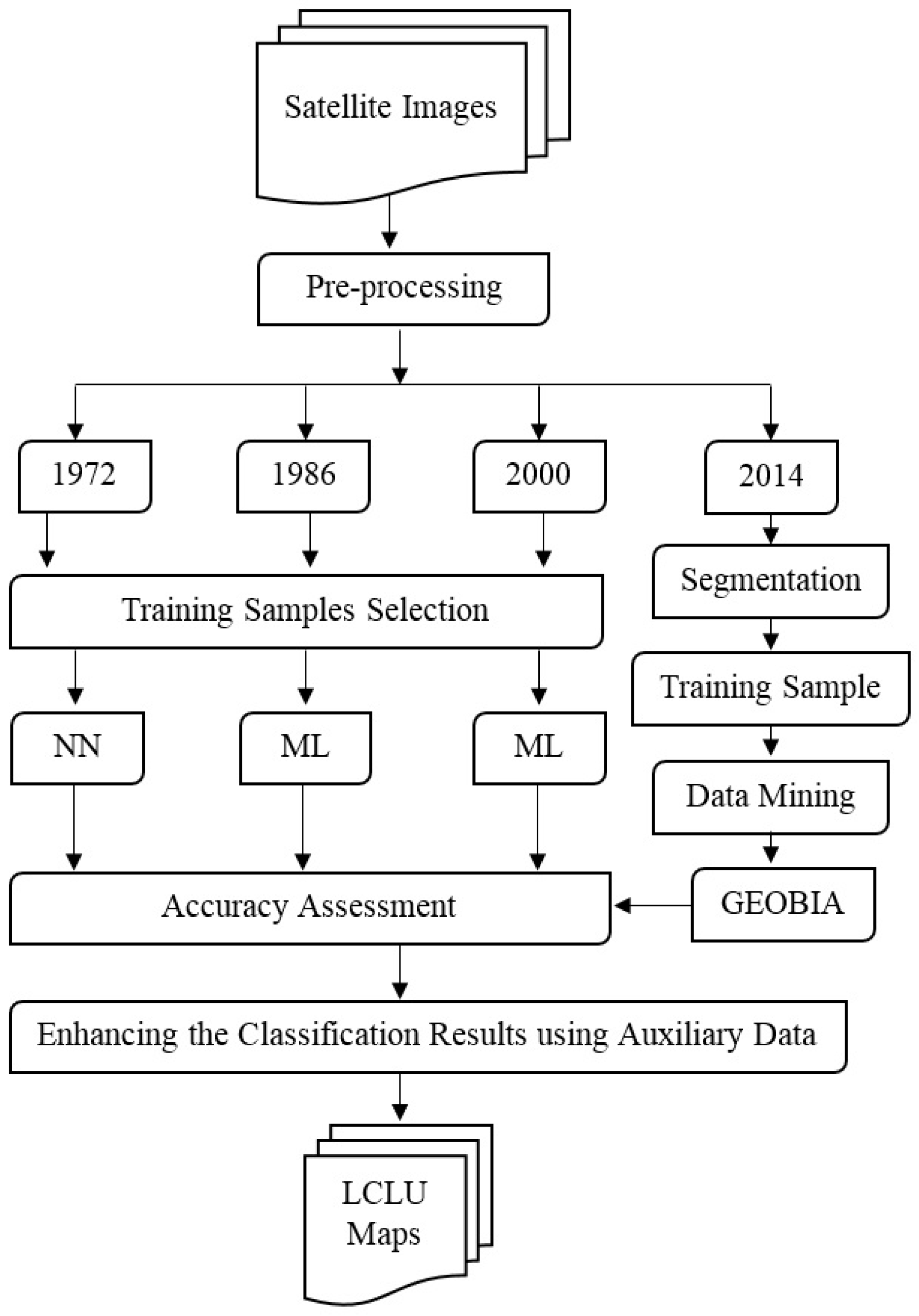
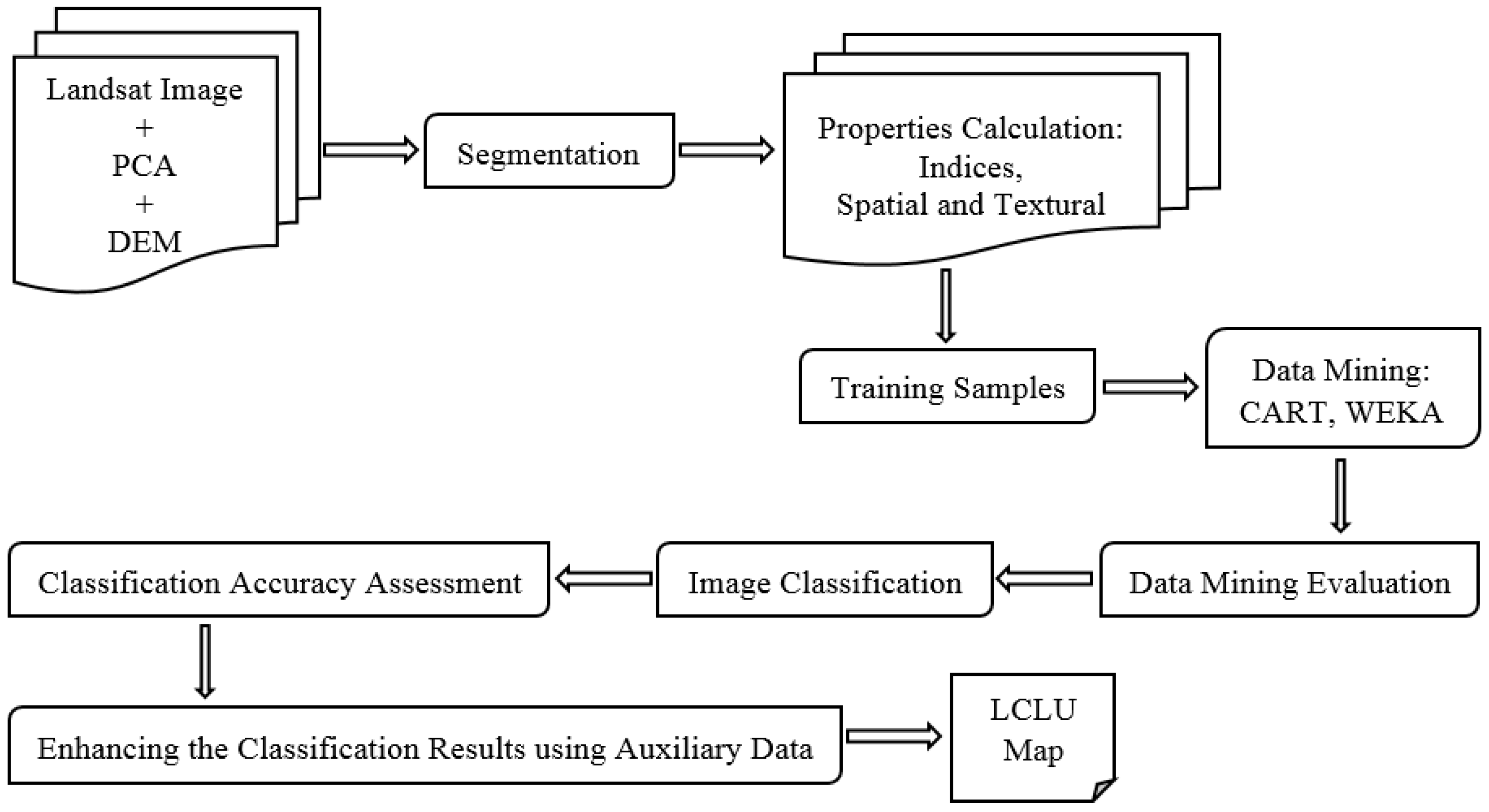
2. Materials and Methods
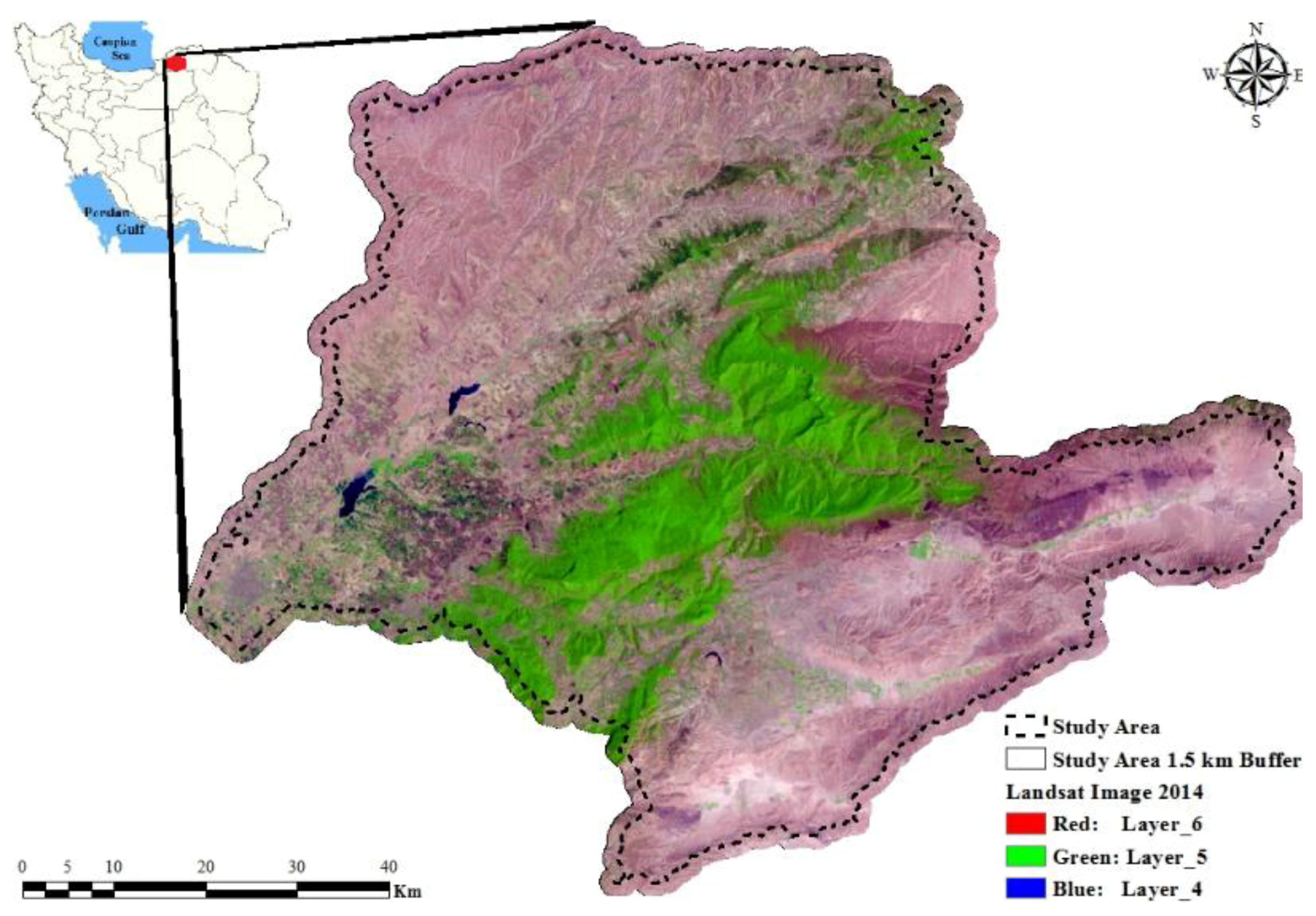
Change detection studies use remote-sensing data as a crucial source of information [17], and classifying the images obtained is a key step in most LCLU analyses. In this regard, we used a number of different ways to classify the satellite images obtained for this study, as shown in Figure 1.

2.1. Study Area

The study area is located in the northeast of Iran and covers an area of 5500 km2 (Figure 2). It is located between the latitudes 36°57′N and 37°47′N, and the longitudes 55°08′E and 56°25′E, and contains the upstream parts of the GW. Altitudes in the area range between 15 and 2541 m above sea level. The area is very important for several reasons, including its agricultural production activities and fertile soils, and has a population of about 600,000 people [7]. It also contains the Golestan National Park, a UNESCO heritage site containing ancient forests, and a large range of flora and fauna species, some of which are endangered and might suffer due to any LCLU changes taking place there. The main plant species of the region include the broadleaf Fagus orientalis, chestnut-leaved oak, Carpinus betulus, Acer cappadocicum and elm zelkova, etc [18]. In addition, this area enjoys agricultural products such as wheat, cotton, oil seeds, grains, etc. Moreover, the study area is geographically complex, and reveals large climatic variation. The plains are located in the east and center; to the south, the area is covered by dense forests and dry highlands, while the north mostly contains hills and is semi-arid [19]. For this study, the selected area was buffered using a 1.5 km distance and all the images were a subset of this buffer boundary. This buffer covered the entire study area to achieve a more accurate classification.

2.2. Datasets

When selecting the most appropriate remote-sensing images to use, a number of factors such as the complexity of the area, coverage, the study’s objectives, user requirements and data availability needed to be considered [20]. The consideration of these factors led to the use of four multi-temporal cloud free L1T Landsat MSS, TM, ETM+ and OLI/TIRS images (Path/Row 162/34) covering the period 1972 to 2014, eventually distributed by the Land Processes Distributed Active Archive Center (LP DAAC) as the core LCLU classification data. In addition, to support the classification, some auxiliary data were used alongside the Landsat data, as shown in Table 1. Google Earth, Yahoo and Bing satellite images offer some advantages in terms of classification, though it should be mentioned that in different areas of the GW, each of these data sources provided distinctive images depending on the time and spatial resolution of the images available. As a result, we used all of these sources together at the same time to increase accuracy. Moreover, a field trip was carried out in May 2013 to collect GCPs and better understand the study area on the ground.

2.3. Image Preprocessing and Pan-Sharpening

The four L1T Landsat images were converted to radiance followed by reflectance, using Equations (1) and (2). More details regarding the equations used can be found in publications [21,22,23].
L λ = G a i n × P i x e l   v a l u e + o f f s e t
ρ λ = π L λ d 2 E S U N λ  sin  θ
where: Lλ is the radiance in units of watts/(meter squared * ster * µm); d is the Earth-Sun distance in astronomical units; ESUNλ is the solar irradiance in units of watts/(meter squared * µm) and θ is the sun elevation in degrees.
We also applied a dark object subtraction model [24] on the images using a methodology commonly applied to reduce atmospheric effects [10].
Pan-sharpening techniques are useful for enhancing the process and results of image processing, and help provide a better understanding of the observed earth surface [14,25]. There are numerous pan-sharpening methods to use on satellite images: high pass filter (HPF), modified intensity-hue-saturation (M-IHS), Ehlers and Gram-Schmidt (GS) [25,26,27,28]. The GS pan-sharpening method has become one of the most prevalent approaches to use on multispectral lower resolution images [27]; therefore, the images for 2000 and 2014 that had pan bands in this study were pan-sharpened with the GS pan-sharpening algorithm.

2.4. Classification

Remote sensing has become a fundamental source of data in geographical studies (e.g., LCLU change research studies), and various classification methods have been developed to extract information from imageries. These methods can be classified into two main types: pixel-based and object-based methods. Pixel-based methods can be unsupervised (based on cluster analysis) or supervised. The latter group uses statistical (e.g., maximum likelihood) and non-statistical algorithms (e.g., neural networks and support vector machines) [20], and each of these has its own advantages and disadvantages. We applied both of them to the images used in this study and chose those which gave the best output. The object-based classification, meanwhile, is a more recently introduced classification method, and overcomes some of the particular problems encountered with pixel-based classification, such as the salt-and-pepper effect [29]. We used the pixel-based classification method for the 1972 to 2000 images, and the object-based classification method for the 2014 image.

2.4.1. Pixel-Based Classification

When recognizing and mapping LCLU change, it is obviously extremely important to determine the number of LCLU classes, and then use the best method to detect them [10]. With this in mind, based on conditions in the study area and other studies that had used Landsat images, such as [30] and [31], we decided to use six classes, including: built-up areas, farmland, bare land, range land, forests and water bodies. These six classes were subsequently used with both the pixel-based and object-based classification methods.
A total of 396 patches were collected, including 240 samples for training and 156 samples for validation. For each of these classes, training areas were carefully selected in the different band combination color composites of each image using different sources including field GCPs, CORONA, QuickBird, Aster images, aerial photos and topographic maps, with Google Earth, Yahoo and Bing satellite maps used as references. Afterwards, the training samples selected were tested for separability, to see how well separated they were. The separation results came out between 0 and 2 for a comparison of each couple, with a very good separation characterized by a value of 1.9 to 2, and a very low separation represented by a value of less than 1 [10].
Supervised classifications, using the maximum likelihood, neural network, support vector machine and other classifiers, were carried out on the images as soon as the classification and training sample grouping had been finalized. After that, we checked the accuracy of the classification results based on the overall accuracy, to assess the quality of the classified images. For this accuracy assessment, different randomly well-distributed samples were collected from the previously mentioned auxiliary data sources, plus a confusion matrix was used to provide accuracy measurements, before selecting the best classification output. Table 2 shows the selected classifier algorithms for each image.
To implement the neural network classifier for the 1972 image, we kept constant the training threshold contribution, rate, momentum and interactions at 0.9, 0.2, 0.9 and 1000, respectively. In contrast, we tried different activation functions (logistic and hyperbolic) and changed the number of hidden layers (one and two, according to [10]). Finally, the combination of constant elements and a hidden layer and logistic function provided the best result.

2.4.2. Geographic Object Based Image Analysis

Over the last two decades, advances in earth observation sensors, computer technology and GI science have led to the development of Geographic Object-Based Image Analysis (GEOBIA) as an alternative to the traditional pixel-based image analysis method [32,33]. In [34] they said that “GEOBIA is a systematic framework for geographic object identification, which combines pixels with the same semantic information into an object, thereby generating an integrated geographic object.” GEOBIA is a newly developed area of Geographic Information Science and remote sensing in which the automatic segmentation of images into objects of similar spectral, temporal and spatial characteristics is carried out [35]. In contrast to traditional image analysis, GEOBIA works more like the human eye–brain combination [33]. The latter compares an object’s properties such as color, square fit, texture, shape and occurrence with other image objects, along with many other properties, to interpret and analyze what the human eye sees [33,35].

Segmentation

GEOBIA starts by segmenting the image grouping pixels into objects, then uses a wide range of object properties to classify the objects or extract object properties from the image [33,36,37]. Multi-resolution segmentation is a popular method of segmentation in the remote-sensing field [36]. To create objects from pixels, some parameters are particularly important, including scale, color and shape, as is the shape’s compactness and smoothness [4]. In most studies to date, the selection of parameter values has been done on a trial and error basis [4]. However, we used the ESP tool [38] to calculate the preferred size of the scale parameters. Different values were tested with regard to different geographical object classes, with the optimal values selected based on scale, shape and compactness at 75, 0.5 and 0.9, respectively. The objects created based on these settings were used for further analysis. For more details on segmentation parameters, we refer readers to a range of studies, including [29,39,40,41].

Data Mining

Generally, the steps followed during a data-mining exercise include image segmentation, training object sampling, data mining of the samples, an evaluation of the output of data-mining activities, image classification, and then a classification accuracy assessment. The whole process is graphically presented in Figure 3.
To provide inputs for the data mining used in this study, section segmentation was applied to the datasets. After that, the data were parameterized based on the LCLU classification requirements. To detect different classes in the image and prepare good criteria for the data-mining process, we calculated Brightness, the Max.diff index (“the absolute difference between the minimum object mean and the maximum object mean divided by the mean object brightness” [36]), and different indices such as NDVI, NDGRVI, NDBI, GNDVI, LWM, NDMI and SLAVI from the 2014 image, plus carried out principal component analysis (PCA). Slope and aspects were derived from the Digital Elevation Model (DEM). The different spatial, textural and spectral characteristics of the objects used as part of the data-mining process (115 properties) were developed, as shown in Table 3.
Subsequently, the 4495 samples were divided into different land classes, these being: bare land, built-up area, farmland, forest land, range land and water bodies. These classes were chosen to provide classification rule-sets for the data miners.
Rule-sets play an important role in the classification of remote-sensing data used in GEOBIA. The data-mining section of the analysis involves the choice and use of intelligent techniques in order to identify and extract patterns of interest of use in the effective production of knowledge [42], where knowledge is understood to mean the behavior patterns identified for each class of interest. We used two data-mining packages: WEKA (Waikato Environment for Knowledge Analysis) [43] and CART (Classification and Regression Trees) [44,45,46] to mine the data and create a rule set for this research.
CART is a non-parametric method that uses a systematic procedure to find ripping rules [47]. It includes seven single-variable splitting criteria: Gini, Sym-Gini, Twoing, Ordered Twoing, Class Probability for classification trees, Least Squares and Least Absolute Deviation for regression trees, and also one multi-variable splitting criterion–the Linear Combinations method [46]. The Gini splitting criteria is the default method. Twoing; meanwhile, is a unique part of the CART method that is normally used for computer modeling, and is suitable for use with classification problems in which there are many classes [46,47]. More details of CART can be found in the studies by [44,45,46,47,48].
The J48 decision tree algorithm was applied here using Waikato Environment for Knowledge Analysis (WEKA), which uses a collection of machine-learning algorithms for its data-mining procedures [42,43,49,50]. The J48 algorithm represents an implementation of C4.5 which selects a property to divide the data into two sub-groups based on the highest normalized information gain (difference in the concept of information entropy). Procedure replication is then applied to each subset until all the cases in each subset fit to the same class. As a result, this procedure creates a leaf node in the decision tree [42,51]. More comprehensive details of the WEKA and J48 applications can be found in [42,43,49,50,52].
To establish the best knowledge model, we evaluated the data-mining results using a standard statistics tool to carry out cross-validation. k-fold cross-validation entails separating a dataset into k accidentally complementary subsets [42]. We used a 10-fold cross-validation process among the training samples, with 10% of the data used for testing and 90% for training. Afterward, the prepared rule set by the machine-learning algorithms were applied to the images. As part of a quality assessment, the accuracy of the classification results was checked based on the overall accuracy, quantity disagreement and allocation disagreement indexes [53].
Although at the end of the classification and accuracy assessment process the LCLU maps created were acceptable, using the auxiliary data we tried to increase the quality of the classification as much as possible through post-processing.

2.5. Accuracy Assessment

As has already been noted, the LCLU maps produced from the pixel- and object-based classifications were assessed for their accuracy. To do so, then, in addition to their overall accuracy assessed based on [53] quantity disagreement and allocation disagreement indexes, other more appropriate statistical tests were also selected and implemented, both for the maps and the reference samples [54]. These indexes were seen as more appropriate because they are able to consider the affiliation between the appropriateness of test samples, as well as their categories and area [54]. According to [53], quantity disagreement is the value of alteration among reference samples and a created map, due to the less-than-optimum match in the proportions of the classes. Allocation disagreement, however, is the amount of spatial deviation seen among classified class pixels taken from validation samples [53,55]. In this study, for the pixel-based classification, 156 samples were selected for each image. For the object-based classification, more than 150 random, well-distributed samples were selected, the samples having been obtained from information gathered during field visits and from all other previously mentioned auxiliary data. For example, using photo interpretation, CORONA satellite images, historical aerial photos and also old topographic maps proved useful for the 1972 and 1986 test samples. For 2000 and 2014, meanwhile, QuickBird and Aster satellite images, along with historical and up-to-date satellite images taken from Google Earth, Yahoo and Bing, provided useful information during the sample selection process.

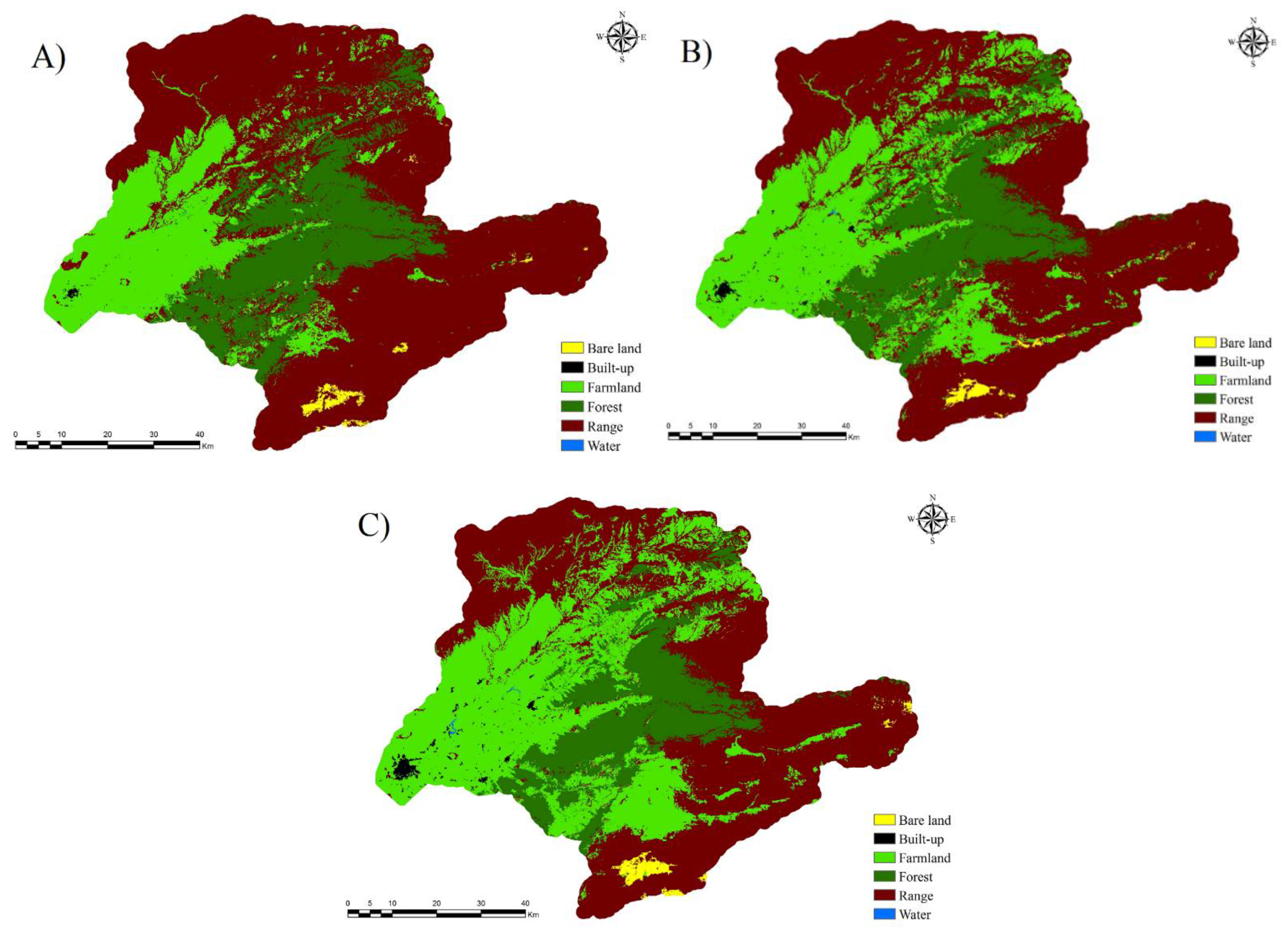
3. Results and Discussion

3.1. Pixel-Based classification

There were 156 well-distributed random samples used as ground-based data to measure the accuracy of the classification. Figure 4 shows the results of the 1972, 1986 and 2000 image classification processes. The results of the accuracy assessment process for the classifications, including quantity and allocation disagreements and overall accuracy levels, are provided in Table 4. As can be seen from the table, the overall accuracy of the maps ranged from 89.8% for 1986 to 95.9% for 1972. The quantity disagreement for 1972—that is, the difference between the number of pixels in the reference map and in a comparison map—was 2.4%, while for 1986 and 2000, it was around 6%. Meanwhile, the allocation disagreement related to the spatial classification difference among categories ranged from 2.2% to 2.7%. The results shown in Table 4 indicate that the accuracy of the spatial classification was more than the quantitative accuracy. Nevertheless, visual interpretation was integrated into the classification results within the GIS environment, to enhance the quality of the final maps.

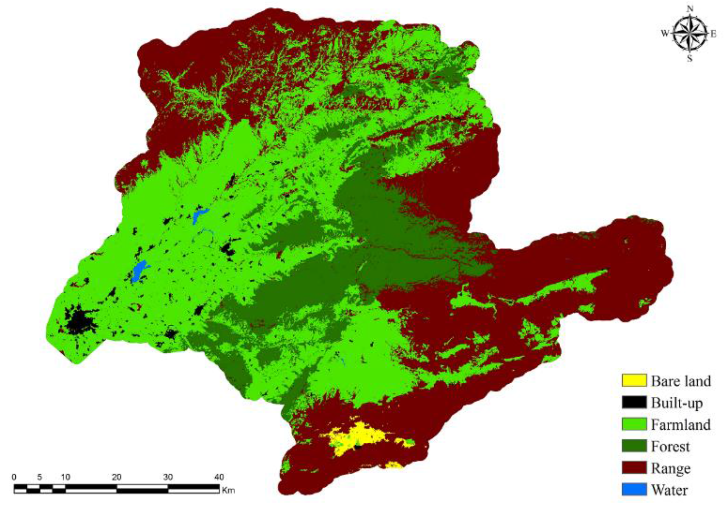
3.2. GEOBIA Classification

Data-mining tools processed the data and detected those attributes deemed important for the building of decision trees. The attributes detected are listed in Table 5.
Applying Gini and J48 algorithms to the training set data presented in Table 3 and using CART and WEKA machine-learning tools allowed the authors to develop decision trees based on the attributes listed in Table 5. Figure 5, meanwhile, shows the decision trees generated by CART and WEKA. To produce precise decision trees, cross-validation was applied during the data-mining process. The overall accuracy of the CART and WEKA data was 96.21% and 96.92%, respectively. As is clear, such levels of accuracy were acceptable, so the results were evaluated after applying decision trees to the 2014 image.
The accuracy of the results was evaluated by creating a confusion matrix, for which 150 randomly distributed and separate samples were used. The results of this process are presented in Table 6. It can be seen from the data in Table 6 that the overall accuracy of the maps was similar, as both attained 94% accuracy. The quantity disagreement shown for WEKA was 2.1%, while when using CART it was 3.5%. Meanwhile, the allocation disagreement was 2.1% for WEKA and 2.5% for CART. As shown in Table 6, both methods revealed the same level of overall accuracy and thus could be considered acceptable. In the end, the WEKA output—due to better allocation and quantity accuracy—was selected and the post-processing corrections applied to provide a more accurate final LCLU map for 2014 (Figure 6).
Both the pixel-based and object-based methods have advantages and disadvantages. The “salt-and-paper issue” plays a significant role in the pixel-based classification methodology, whereas the rule construction process within GEOBIA analysis is often difficult to perform. However, for the object-based method, its machine-learning and data-mining abilities facilitate rule creation and subsequently image classification. A comparison of the two classification methods reveals that the range of overall accuracy variation in the two object-based classifications is less than three pixel-based ones. Moreover, quantity disagreement for the pixel-based classification method is greater than when using the object-based approach. Nonetheless, allocation disagreement levels for both methods are approximately within the same range.
The results of the classification process for each year provided an overall estimate of LCLU distribution in the study area. As shown in Figure 4 and Figure 6, and as can be seen clearly in Table 7, different classes covered different areas over the years involved. It is apparent from the tables and figures that in 1972, 1986 and 2000, rangeland was the dominant land cover type, covering ~60%, 50% and 45% of the area, respectively. Farmland and forest expanded the most over the period 1972 to 2000, following the LC range. From Table 7, a significant difference can be seen between 2014 and previous years, because rangeland stopped being the most dominant land cover, having been replaced by farmland (40%). In 2014, farmland, rangeland and then forestland were the most dominant land cover types, in that order. Over the whole period, water bodies and built-up land covered the smallest areas (maximums of 1.45% and 0.19%, respectively).
From 1972 to 2014, rangeland, the most prevalent class, was largely converted into farmland (more than 26 million ha) and forest (~2 million ha). The latter conversion can be linked to the establishment of the Golestan National Park and the provision of different energy resources for the local population, as well as to reforestation and afforestation activities. Furthermore, during these years, about 5 million ha of forest surface that had for the most part been located close to built-up and flat land were also converted to farmland. Farmland surfaces were mainly converted to built-up areas (approximately 1.3 million ha) and water bodies (more than 200,000 ha); such changes were concentrated in parts of the region covered by plains. However, the expansion of built-up areas was not only to the detriment of farmland; it also took around 465,000 ha from rangelands and 30,000 ha from forests over the period 1972 to 2014. At the same time, barren areas expanded by taking approximately 456,000 ha from rangelands (Table 8). Similarly, [13] who studied tree cover changes during 1987–2001 in part of the study area, found that the forest areas had decreased.

4. Conclusion

This study set out to determine Land Cover/Land Use (LCLU) statuses over the period 1972 to 2014 (a period of 42 years) for the Gorganrood watershed in the northeast of Iran. Based on pixel-based remote-sensing and supervised classifications, and including the use of neural network and maximum likelihood methods, the authors created land use maps for the period 1972 to 2000. After that, a combination of GEOBIA remote-sensing and data-mining methods provided the framework needed for the LCLU mapping process to take place, and this was then also applied to a 2014 image. Both pixel-based and object-based classification methods have both advantages and disadvantages. For example, pixel-based classifications suffer from the salt-and-paper problem, while performing rule construction activities using GEOBIA analysis is often difficult. However, using data mining with the object-based method can facilitate rule-set creation and subsequently image classification, and provide a stable level of accuracy in different classifications.
With the LCLU maps obtained, the authors were able to clarify LCLU status over the study period, showing that in 1972, 1986 and 2000, rangeland was the dominant land cover type. Meanwhile, farmland and forestland expanded the most over the period, following the LC range. There was a significant difference found between 2014 and the previous dates tested, as by this time rangeland was no longer the dominant land cover type, having been replaced by farmland, followed by rangeland and then forestland. Over the whole period, water bodies and built-up land covered the smallest areas.
The results of this study indicate that a significant amount of change has occurred in the watershed since 1972, and that this had effect on the area’s ecosystems and human livelihoods. In the Gorganrood watershed flood, landslide and land subsidence are dominant natural hazards and, based on the various influences of LCLU on these processes, increases in farmland and built-up areas, in addition to decreases in forestland and rangeland, may well have increased the number and type of natural hazards, especially floods, as flooding predominates in the region. The local and national governments and decision makers can use the study outcomes to understand the nature and location of the LCLU changes that have occurred, and consider these changes when developing future plans and projects to mitigate natural hazards. Using the improved knowledge of LCLU statuses in the area generated by this study, it is recommended that more research be carried out in order to understand the dynamics of and relations among LCLU classes, so that the watershed can be managed more effectively in the future. Also, further studies regarding the impact of LCLU changes on the future of the watershed should be considered, to help improve our knowledge in this area and help manage the future more efficiently.

Acknowledgments

Images were retrieved from the online Data Pool, courtesy of the NASA Land Processes Distributed Active Archive Center (LP DAAC), and the USGS/Earth Resources Observation and Science (EROS) Center in Sioux Falls, South Dakota (https://lpdaac.usgs.gov/data_access/data_pool). In addition, we appreciate the help provided by Seyed Reza Hosseinzadeh and Sajad Bagheri. We are grateful for the constructive comments given by Robert Gilmore Pontius, Jr. and the three anonymous reviewers of our paper.

Author Contributions

Masoud Minaei came up with the research idea and Wolfgang Kainz provided guidance on the overall project. The study was carried out and the initial version of the paper was written by Masoud Minaei. Wolfgang Kainz supervised the entire research, provided valuable advice and made key modifications to the paper. The paper was revised by both.

Conflicts of Interest

The authors declare no conflict of interest.

References

  1. Thilagavathi, N.; Subramani, T.; Suresh, M. Land use/land cover change detection analysis in Salem Chalk Hills, South India using remote sensing and GIS. Disaster Adv. 2015, 8, 44–52. [Google Scholar]
  2. Adhikari, S.; Southworth, J.; Nagendra, H. Understanding forest loss and recovery: A spatiotemporal analysis of land change in and around Bannerghatta National Park, India. J. Land Use Sci. 2014, 10, 1–23. [Google Scholar] [CrossRef]
  3. Lambin, E.F.; Turner, B.L.; Geist, H.J; Agbola, S.B.; Angelsen, A.; Bruce, J.W.; Coomes, O.T.; Dirzo, R.; Fischer, J.; Folke, C.; et al. The causes of land-use and land-cover change: Moving beyond the myths. Glob. Environ. Chang. 2001, 11, 261–269. [Google Scholar] [CrossRef]
  4. Dingle Robertson, L.; King, D.J. Comparison of pixel- and object-based classification in land cover change mapping. Int. J. Remote Sens. 2011, 32, 1505–1529. [Google Scholar] [CrossRef]
  5. Chapin Iii, F.S.; Zavaleta, E.S.; Eviner, V.T.; Naylor, R.L.; Vitousek, P.M.; Reynolds, H.L.; Hooper, D.U.; Lavorel, S.; Sala, O.E.; Hobbie, S.E.; et al. Consequences of changing biodiversity. Nature 2000, 405, 234–242. [Google Scholar] [CrossRef] [PubMed]
  6. Berakhi, R.O.; Oyana, T.J.; Adu-Prah, S. Land use and land cover change and its implications in Kagera river basin, East Africa. Afr. Geogr. Rev. 2014, 34, 1–23. [Google Scholar] [CrossRef]
  7. Statistical-Center-of-Iran. Iranian Population and Housing Census 1385—Golestan Province General Results; Statistical-Center-of-Iran: Tehran, Iran, 2006. [Google Scholar]
  8. Qin, Y.; Niu, Z.; Chen, F.; Li, B.; Ban, Y. Object-based land cover change detection for cross-sensor images. Int. J. Remote Sens. 2013, 34, 6723–6737. [Google Scholar] [CrossRef]
  9. Yesmin, R.; Mohiuddin, A.S.M.; Uddin, M.J.; Shahid, M.A. Land use and land cover change detection at Mirzapur Union of Gazipur District of Bangladesh using remote sensing and GIS technology. In Proceedings of the IOP Conference Series: Earth and Environmental Science, Kuala Lumpur, Malaysia, 22–23 April 2014.
  10. Kolios, S.; Stylios, C.D. Identification of land cover/land use changes in the greater area of the Preveza peninsula in Greece using Landsat satellite data. Appl. Geogr. 2013, 40, 150–160. [Google Scholar] [CrossRef]
  11. Abd El-Kawy, O.R.; Rød, J.K.; Ismail, H.A.; Suliman, A.S. Land use and land cover change detection in the western Nile delta of Egypt using remote sensing data. Appl. Geogr. 2011, 31, 483–494. [Google Scholar] [CrossRef]
  12. Yang, X.; Lo, C.P. Using a time series of satellite imagery to detect land use and land cover changes in the Atlanta, Georgia metropolitan area. Int. J. Remote Sens. 2002, 23, 1775–1798. [Google Scholar] [CrossRef]
  13. Salman Mahini, A.; Feghhi, J.; Nadali, A.; Riazi, B. Tree cover change detection through Artificial Neural Network classification using Landsat TM and ETM+ images (case study: Golestan Province, Iran). Iran. J. For. Poplar Res. 2008, 16, 495–505. [Google Scholar]
  14. Saadat, H.; Adamowski, J.; Bonnell, R.; Sharifi, F.; Namdar, M.; Ale-Ebrahim, S. Land use and land cover classification over a large area in Iran based on single date analysis of satellite imagery. ISPRS J. Photogramm. Remote Sens. 2011, 66, 608–619. [Google Scholar] [CrossRef]
  15. Abbaszadeh Tehrani, N.; Makhdoum, M.F.; Mahdavi, M. Studying the impacts of land use changes on flood flows by using remote sensing(RS) and geographical information system (GIS) techniques—A case study in dough river watershed, Northeast of Iran. Environ. Res. 2011, 1, 1–14. [Google Scholar]
  16. Mallinis, G.; Koutsias, N.; Arianoutsou, M. Monitoring land use/land cover transformations from 1945 to 2007 in two peri-urban mountainous areas of Athens metropolitan area, Greece. Sci. Total Environ. 2014, 490, 262–278. [Google Scholar] [CrossRef] [PubMed]
  17. Lu, D.; Mausel, P.; Brondízio, E.; Moran, E. Change detection techniques. Int. J. Remote Sens. 2004, 25, 2365–2401. [Google Scholar] [CrossRef]
  18. Mohammadi, J.; Shataee, S. Possibility investigation of tree diversity mapping using Landsat ETM+ data in the Hyrcanian forests of Iran. Remote Sens. Environ. 2010, 114, 1504–1512. [Google Scholar] [CrossRef]
  19. Delbari, M.; Afrasiab, P.; Jahani, S. Spatial interpolation of monthly and annual rainfall in northeast of Iran. Meteorol. Atmos. Phys. 2013, 122, 103–113. [Google Scholar] [CrossRef]
  20. Lu, D.S.; Li, G.Y.; Kuang, W.H.; Moran, E. Methods to extract impervious surface areas from satellite images. Int. J. Digit. Earth 2014, 7, 93–112. [Google Scholar] [CrossRef]
  21. USGS. Using the USGS Landsat 8 Product. Available online: http://landsat.usgs.gov/Landsat8_Using_Product.php (accessed on 10 March 2015).
  22. USGS. How is Radiance Calculated? Available online: http://landsat.usgs.gov/how_is_radiance_calculated.php (accessed on 12 March 2016).
  23. Exelis VIS, p.d.c. Radiometric Calibration. Available online: http://www.exelisvis.com/docs/RadiometricCalibration.html (accessed on 12 March 2016).
  24. Chavez, P.S. Radiometric calibration of Landsat thematic mapper multispectral images. Photogramm. Eng. Remote Sens. 1989, 55, 1285–1294. [Google Scholar]
  25. Yuhendra; Alimuddin, I.; Sumantyo, J.T.S.; Kuze, H. Assessment of pan-sharpening methods applied to image fusion of remotely sensed multi-band data. Int. J. Appl. Earth Obs. Geoinform. 2012, 18, 165–175. [Google Scholar] [CrossRef]
  26. ArcGIS Help. Fundamentals of Panchromatic Sharpening. Available online: http://resources.arcgis.com/en/help/main/10.1/index.html#//009t000000mw000000 (accessed on 11 March 2015).
  27. Maurer, T. How to pan-sharpen images using the Gram-Schmidt pan-sharpen method-a recipe. Int. Arch. Photogramm. Remote Sens. Spat. Inf. Sci. 2013, XL-1/W1, 239–244. [Google Scholar] [CrossRef]
  28. Laben, C.A.; Brower, B.V. Process for Enhancing the Spatial Resolution of Multispectral Imagery using Pan-Sharpening. Google Patents US6011875 A, 2000. [Google Scholar]
  29. Blaschke, T. Object based image analysis for remote sensing. ISPRS J. Photogramm. Remote Sens. 2010, 65, 2–16. [Google Scholar] [CrossRef]
  30. Nutini, F.; Boschetti, M.; Brivio, P.A.; Bocchi, S.; Antoninetti, M. Land-use and land-cover change detection in a semi-arid area of Niger using multi-temporal analysis of Landsat images. Int. J. Remote Sens. 2013, 34, 4769–4790. [Google Scholar] [CrossRef]
  31. Wu, G.; Gao, Y.; Wang, Y.; Wang, Y.Y.; Xu, D. Land-use/land cover changes and their driving forces around wetlands in Shangri-La County, Yunnan Province, China. Int. J. Sustain. Dev. World Ecol. 2015, 22, 110–116. [Google Scholar] [CrossRef]
  32. Gao, Y.; Mas, J.F. A comparison of the performance of pixel based and object based classifications over images with various spatial resolutions. ISPRS Arch. 2008, XXXVIII-4/C1, 1–6. [Google Scholar]
  33. Addink, E.A.; van Coillie, F.M.B.; de Jong, S.M. Introduction to the GEOBIA 2010 special issue: From pixels to geographic objects in remote sensing image analysis. Int. J. Appl. Earth Obs. Geoinf. 2012, 15, 1–6. [Google Scholar] [CrossRef]
  34. Ma, L.; Cheng, L.; Li, M.; Liu, Y.; Ma, X. Training set size, scale, and features in geographic object-based image analysis of very high resolution unmanned aerial vehicle imagery. ISPRS J. Photogramm. Remote Sens. 2015, 102, 14–27. [Google Scholar] [CrossRef]
  35. Rabia, A.H.; Terribile, F. Semi-automated Classification of gray scale aerial photographs using geographic object based image analysis (GEOBIA) technique. In European Geosciences Union General Assembly-Geophysical Research Abstracts; Vienna, Austria, 2013. [Google Scholar]
  36. Blaschke, T.; Feizizadeh, B.; Holbling, D. Object-based image analysis and digital terrain analysis for locating landslides in the urmia lake basin, Iran. IEEE J. Sel. Top. Appl. Earth Obs. Remote Sens. 2014, 7, 4806–4817. [Google Scholar] [CrossRef]
  37. Witharana, C.; Civco, D.L.; Meyer, T.H. Evaluation of data fusion and image segmentation in earth observation based rapid mapping workflows. ISPRS J. Photogramm. Remote Sens. 2014, 87, 1–18. [Google Scholar] [CrossRef]
  38. Dragut, L.; Tiede, D.; Levick, S.R. ESP: A tool to estimate scale parameter for multiresolution image segmentation of remotely sensed data. Int. J. Geogr. Inf. Sci. 2010, 24, 859–871. [Google Scholar] [CrossRef]
  39. Wang, Z.; Jensen, J.R.; Im, J. An automatic region-based image segmentation algorithm for remote sensing applications. Environ. Model. Softw. 2010, 25, 1149–1165. [Google Scholar] [CrossRef]
  40. Lang, S. Object-based image analysis for remote sensing applications: Modeling reality–dealing with complexity. In Object-Based Image Analysis; Blaschke, T., Lang, S., Hay, G., Eds.; Springer: Berlin, Germany, 2008; pp. 3–27. [Google Scholar]
  41. Baatz, M.; Schäpe, M. Multiresolution segmentation. In Angewandte Geographische Informations-Verarbeitung; Strobl, J., Blaschke, T., Griesebner, G., Eds.; Wichmann Verlag: Karlsruhe, Germany, 2000; pp. 12–23. [Google Scholar]
  42. Vieira, M.A.; Formaggio, A.R.; Renno, C.D.; Atzberger, C.; Aguiar, D.A.; Mello, M.P. Object based image analysis and data mining applied to a remotely sensed Landsat time-series to map sugarcane over large areas. Remote Sens. Environ. 2012, 123, 553–562. [Google Scholar] [CrossRef]
  43. Hall, M.; Frank, E.; Holmes, G.; Pfahringer, B.; Reutemann, P.; Witten, I.H. The WEKA data mining software: An update. SIGKDD Explor. Newslett. 2009, 11, 10–18. [Google Scholar] [CrossRef]
  44. Breiman, L.; Friedman, J.; Olshen, R.; Stone, C. Classification and Regression Trees; Pacific Grove: Wadsworth, OH, USA, 1984. [Google Scholar]
  45. Steinberg, D.; Colla, P. Cart-Classification and Regression Tree; Salford Systems: San Diego, CA, USA, 1997. [Google Scholar]
  46. Dan Steinberg, M.G. CART 6.0 User’s Manual; Salford Systems: San Diego, CA, USA, 2006. [Google Scholar]
  47. Waheed, T.; Bonnell, R.B.; Prasher, S.O.; Paulet, E. Measuring performance in precision agriculture: CART—A decision tree approach. Agric. Water Manag. 2006, 84, 173–185. [Google Scholar] [CrossRef]
  48. Salford System. CART Classification and Regression Trees; Salford Systems: San Diego, CA, USA, 2015. [Google Scholar]
  49. Sharma, R.; Ghosh, A.; Joshi, P.K. Decision tree approach for classification of remotely sensed satellite data using open source support. J. Earth Syst. Sci. 2013, 122, 1237–1247. [Google Scholar] [CrossRef]
  50. Biswal, S.; Ghosh, A.; Sharma, R.; Joshi, P.K. Satellite data classification using open source support. J. Indian Soc. Remote Sens. 2013, 41, 523–530. [Google Scholar] [CrossRef]
  51. Kramer, S. J48. Available online: http://www.opentox.org/dev/documentation/components/j48/ (accessed on 12 March 2016).
  52. Waikato, M.L.G. Weka 3: Data Mining Software in Java. Available online: http://www.cs.waikato.ac.nz/~ml/weka/ (accessed on 12 March 2016).
  53. Pontius, R.G., Jr.; Millones, M. Death to Kappa: Birth of quantity disagreement and allocation disagreement for accuracy assessment. Int. J. Remote Sens. 2011, 32, 4407–4429. [Google Scholar] [CrossRef]
  54. Cordeiro, C.L.D.; Rossetti, D.D. Mapping vegetation in a late quaternary landform of the Amazonian wetlands using object-based image analysis and decision tree classification. Int. J. Remote Sens. 2015, 36, 3397–3422. [Google Scholar] [CrossRef]
  55. Mansour, K.; Mutanga, O.; Adam, E.; Abdel-Rahman, E.M. Multispectral remote sensing for mapping grassland degradation using the key indicators of grass species and edaphic factors. Geocarto Int. 2016, 31. [Google Scholar] [CrossRef]
Figure 1. LCLU mapping flowchart. NN = Neural Network, ML = Maximum Likelihood, GEOBIA = Geographic Object-Based Image Analysis.
Ijgi 05 00057 g001
Figure 2. Study area in the northeast of Iran.
Ijgi 05 00057 g002
Figure 3. GEOBIA and data-mining procedure flowchart.
Ijgi 05 00057 g003
Figure 4. Classification results for: (A) 1972; (B) 1986 and (C) 2000.
Ijgi 05 00057 g004
Figure 5. Schematic decision trees created using the data-mining tools (A) CART and (B) WEKA.
Ijgi 05 00057 g005
Figure 6. LCLU 2014 classification results.
Ijgi 05 00057 g006
Table 1. Data used for the LCLU mapping process.
Data NameAcquisition DateResolutionFull Area CoverageSource
Landsat/MSS20 September 197260 mYeshttp://earthexplorer.usgs.gov/
Landsat/TM19 May 198630 mYeshttp://earthexplorer.usgs.gov/
Landsat ETM+20 July 200030 m (Pan 15)Yeshttp://earthexplorer.usgs.gov/
Landsat OLI/TIRS19 July 201430 m (Pan 15)Yeshttp://earthexplorer.usgs.gov/
Aster18 July 200115 mNohttp://reverb.echo.nasa.gov/
CORONA27 May 1970~2.1 mNohttp://earthexplorer.usgs.gov/
Quickbird20050.6 mNoGeography Department, Ferdowsi University of Mashhad
Aerial Photo1970~1.9 mNoGeography Department, University of Tehran
DEM (Aster)30 mYeshttp://earthexplorer.usgs.gov/
Topographic MapNoGeography Department, University of Tehran
GIS Thematic MapsYes/NoDepartment of Natural Resource and Watershed Management, Golestan
Google/Yahoo/Bing Historical and up to Date ImagesYes/NoInternet
Table 2. Selected classifiers for each image.
ImageClassification MethodClassifier
1972Pixel-basedNeural Network
1986Pixel-basedMaximum Likelihood
2000Pixel-basedMaximum Likelihood
2014Object-BasedRule-based
Table 3. Characteristics of the objects and indices used as part to the data mining process (STDDEV: Standard Deviation; TC: Tasseled Cap; SLAVI: Specific Leaf Area Vegetation Index; NDVI: Normalized Difference Vegetation Index; NDMI: Normalized Dry Matter Index; NDGRVI: Normalized Difference Green Red Vegetation Index; NDBI: Normalized Difference Build-Up Index; LWM: Land and Water Mask; GNDVI: Green Normalized Difference Vegetation Index).
Name of AttributesName of AttributesName of Attributes
Mean and STDDEV of B1Mean and STDDEV of B5-OVER-B4Brightness
Mean and STDDEV of B2Mean and STDDEV of B4-OVER-B6Max Diff
Mean and STDDEV of B3Mean and STDDEV of B4-OVER-B5Modified mean brightness
Mean and STDDEV of B4Mean and STDDEV of B3-OVER-B4Elliptic fit
Mean and STDDEV of B5Mean and STDDEV of DEMCompactness
Mean and STDDEV of B6Mean and STDDEV of ASPECTWidth
Mean and STDDEV of B7Mean and STDDEV of SLOPEAsymmetry
Mean and STDDEV of B8STDDEV of area represented by segmentsDensity
Mean and STDDEV of B9Length width only main lineRectangular fit
Mean and STDDEV of PCA1Relative border to image borderLength
Mean and STDDEV of PCA2Average area represented by segmentLength width
Mean and STDDEV of PCA3STDDEV curvature only main lineAverage branch length
Mean and STDDEV of PCA4Length of longest edge (polygon)Volume
Mean and STDDEV of PCA5Average length of edges (polygon)Perimeter (polygon)
Mean and STDDEV of PCA6Polygon self-intersection (polygon)Length thickness
Mean and STDDEV of PCA7Radius of smallest enclosing ellipseShape index
Mean and STDDEV of TC WetnessArea excluding inner polygonsThickness
Mean and STDDEV of TC GreennessLength of main line regarding cyclesNumber of segments
Mean and STDDEV of TC BrightnessArea including inner polygonsMaximum branch length
Mean and STDDEV of SLAVINumber of inner objects (polygon)Area
Mean and STDDEV of NDVISTDDEV of length of edges (polygon)Border index
Mean and STDDEV of NDMIRadius of largest enclosed ellipseWidth only main line
Mean and STDDEV of NDGRVIDegree of skeleton branchingCompactness (polygon)
Mean and STDDEV of NDBILength of main line no cycleNumber of pixels
Mean and STDDEV of LWMCurvature length only main lineRoundness
Mean and STDDEV of GNDVIBorder LengthMain direction
Mean and STDDEV of B7-OVER-B3Number of edges (polygon)
Table 4. Selected classifiers for each image as well as the overall accuracy, quantity and allocation disagreement statistics.
ImageClassifierOverall AccuracyQuantity Disagreement (%)Allocation Disagreement (%)
1972Neural Network95.92.42.2
1986Maximum Likelihood89.86.62.5
2000Maximum Likelihood91.362.7
Table 5. Attributes detected by CART and WEKA.
AttributesCARTWEKAAttributesCARTWEKA
STDDEV of B1Mean and STDDEV of B6-
Mean of B8Mean and STDDEV of PCA6
STDDEV of B9Mean and STDDEV of TC Greenness
STDDEV of PCA1-Mean of B3-OVER-B4
STDDEV of PCA3Mean and STDDEV of DEM
Mean of PCA4STDDEV of ASPECT-
Mean of PCA5Average area represented by segment-
STDDEV of PCA5-Length of longest edge (polygon)
Mean of PCA7Average length of edges (polygon)
STDDEV of PCA7-Mean and STDDEV of NDGRVI-
STDDEV of SLAVIBrightness
Mean of NDMIMax Diff
Mean of GNDVIModified mean brightness
Mean of SLOPEBorder Length-
Mean of TC Wetness-Mean of B7-
Asymmetry-Mean of NDVI-
Mean LWM-
Table 6. Overall accuracy plus quantity and allocation disagreement statistics for the image classification using the two data-mining methods.
ImageData MinerOverall AccuracyQuantity Disagreement (%)Allocation Disagreement (%)
2014WEKA (J48)94.052.12.1
2014CART (GINI)94.033.52.5
Table 7. Summary of land cover type areas over the study years—per hectare and as a percentage of the total area.
LCLU Class1972198620002014
Area (ha)(%)Area (ha)(%)Area (ha)(%)Area (ha)(%)
Bare Land4404.780.704084.520.655759.800.924305.240.69
Built-up819.070.132646.880.425050.670.819057.291.45
Farmland125,379.0920.02182,633.2729.16224,809.3135.90255,753.5940.84
Forest122,614.2019.58119,333.8619.06106,020.8316.93106,267.8216.97
Range372,998.4559.56317,440.7850.69284,351.4045.41249,663.4039.87
Water20.570.0096.950.02244.280.041,188.970.19
Table 8. Transmission matrix for LCLU changes (ha) over the 1972–2014 period.
1972/2014BarelandBuilt-UpFarmlandForestRangeWater
Bare Land510,780.9411,091.94108,636.190.00360,566.440.00
Built-Up0.00183,500.44263.250.000.00526.50
Farmland0.001,347,779.2526,545,861.6917,177.0671,649.56227,827.69
Forest0.0030,243.384,759,347.3822,014,225.56782,257.502,121.19
Range457,898.06465,264.0026,129,653.311,878,855.7554,959,785.8833,194.81
Water0.000.00779.630.000.003,847.50

