Integrating Spatial and Attribute Characteristics of Extended Voronoi Diagrams in Spatial Patterning Research: A Case Study of Wuhan City in China

Abstract

Rapid urbanization has caused numerous problems, and the urban spatial structure has been a hot topic in sustainable development management. Urban spatial structure is affected by a series of factors. Thus, the research model should synthetically consider the spatial and non-spatial relationship of every element. Here, we propose an extended Voronoi diagram for exploring the urban land spatial pattern. In essence, we first used a principal component analysis method to construct attribute evaluation indicators and obtained the attribute distance for each indicator. Second, we integrated spatial and attribute distances to extend the comparison distance for Voronoi diagrams, and then, we constructed the Voronoi aggregative homogeneous map of the study area. Finally, we make a spatial autocorrelation analysis by using GeoDA and SPSS software. Results show that: (1) the residential land cover aggregation is not significant, but spatial diffusion is obvious; (2) the commercial land cover aggregation is considerable; and (3) the spatial agglomeration degree of the industrial land cover is increased and mainly located in urban fringes. According to the neo-Marxist theory, we briefly analyzed the driving forces for shaping the urban spatial structure. To summarize, our approach yields important insights into the urban spatial structure characterized by attribute similarity with geospatial proximity, which contributes to a better understanding of the urban growth mechanism. In addition, it explicitly identifies ongoing urban transformations, potentially supporting the planning for sustainable urban land use and protection.

1. Introduction

Although urban surfaces currently cover only between 3% and 5% of the total land surface of the Earth, environmental impacts in relation to urban growth have become a major concern around the world [1]. Rapid urban growth due to large-scale land use/cover change, particularly in developing countries, has drawn considerable attention since urbanization drives environmental change at multiple scales [2,3,4,5,6,7]. Recent decades have witnessed unprecedented urban landscape changes, rapid land use changes found in urbanization processes, loss of ecosystems and biodiversity and the exploration of available resources, leading to scarcity [5,6,7,8,9,10,11]. These transformations raise a series of questions: Is our urban spatial structure sustainable development? How can policy most effectively shape urban morphology and manage urban spatial structure, expansion and decline or agglomeration and dispersion? What guidelines should we provide for policymakers and regional planners to note the future development of our urban environment? Addressing such questions requires an explicit model to discover the aggregation tendency of spatial entities, the distribution rules, the development and change tendency and the driving forces for shaping the urban spatial structure from spatial data [12,13].

Urban spatial structure (also known as urban internal spatial structure or urban space) refers to the arrangement of land use in urban areas, which concerns the arrangement of public and private space in cities and the degree of connectivity and accessibility [14]. The characterization and modeling of urban spatial structure has been highlighted as an important research activity in recent years, especially in those countries with rapid urbanization and industrialization, such as China [15,16,17].

In the past, various theories, such as central place theory, core-periphery theory, Losch’s demand cone theory, spatial diffusion theory, growth pole theory, concentric rings theory, sector theory, Zipf’s law and multiple nuclei theory were extensively used to study urban structure patterns and dynamics [1,18,19,20,21,22]. However, urban growth is a complex spatial system, comprised of numerous acting and interacting elements with feedbacks in between, which inevitably determine the overall spatial form of the city [23]. Therefore, these conventional urban geography theories are unable to characterize the spatiotemporal complexity of urban dynamics [1,24,25]. In response, a variety of techniques, such as catastrophe theory, fractals theory, chaos or chaotic attractors theory, self-organizing theory, entropy theory, landscape metrics, cellular automata and agent-based modeling, have emerged since the 1960s to analyze the urban structure and dynamics [1,23,26,27,28,29,30,31].

The modeling of urban spatial structure has occupied researchers for decades, and an abundant literature has emerged. The advancements of mathematical theories and computer-based simulations based on equations to seek a static or equilibrium solution have helped us to better understand cities [24]. Most common mathematical models are sets of simultaneous joint equations based on theories of population growth and diffusion and economic theory that specify cumulative urban spatial structure over time [32,33,34]. A major drawback of such mathematical models is that a numerical or analytical solution to the system of equations must be obtained, limiting the level of complexity that may practically be built into such models [35]. The complex systems science modeling techniques offer a potentially appropriate toolbox, notably agent-based modeling and cellular automata, potentially linked to Geographic Information System (GIS) and Remote Sensing (RS) information on land parcels [1,6,23,36,37,38]. Techniques, such as Cellular Automata (CA), as rule-based models construct a ‘bottom-up’ approach, where the structure evolves from a Moran neighborhood interacting between neighboring cells using different types of transition rules [31,39,40,41]. Moreover, the conventional urban CA model assumption that a regular cell represents the basic unit of a land use entity is not always reasonable [42]. Several studies deal with the development of vector-based or irregular CA models; however, these new kinds of CA models are still in their infancy [43,44].

The spatial structure of some social and economic variables may be a reflection of spillover effects, which usually are evident from the form of spatial association. Agglomeration economies, on the other hand, may produce differential effects over space [45]. In urban studies, this usually means that high variable values tend to concentrate near other high values, and low values appear in geographical proximity. In this sense, spatial association is the non-random ordering of data values when they are arranged by spatial location and can be analyzed by using distance statistics [45,46,47]. Geospatial clustering is a series of processes that groups a distinct point set into a number of groups exhibiting similar characteristics according to the geospatial proximity. Points belonging to the same geospatial cluster are more similar to each other than points belonging to different clusters [48]. Analysis of spatial clustering has been a major topic of research in geographical pattern research [49,50]. Spatial statistics methods were introduced in geology and geography in the 1950s, but have only recently started to serve the purposes and needs of urban analysis, specifically applied to the analysis of urban land prices [51,52,53]. In spatial statistics, spatial data analysis is often categorized into three types, namely point data analysis, lattice data analysis and geostatistics [54]. Geostatistics concerns the spatial pattern of an attribute on a regular or irregular spatial lattice, with an additional goal of predicting the values of the attribute at unsampled locations [54]. Geostatistics uses distance-based functions rather than neighborhood structures to represent spatial autocorrelation, and the detection of clusters is based on local spatial statistics, such as the local Moran’s I statistic. Geostatistical data refer to spatial data sampled at point locations that are continuous in space [54,55,56]. Given a set of a finite number of points in the Euclidean plane, we associate each location in the space with its closest member(s) of the point set with respect to the Euclidean distance. The result is a tessellation of the plane into a set of regions associated with individual members of the point set. This tessellation is called the “ordinary planar Voronoi diagrams”, generated by the sample point set [57]. As one of the spatial data analysis tools, Voronoi diagrams can be used to implement the spatial subdivision and reveal the scope of spatial influence generated by urban areas.

The objective of this study is to identify the urban spatial structure in Wuhan of P.R. China by applying spatial data statistics, Voronoi diagrams, GeoDA and GIS. We consider that our analysis is useful in the following sense. First, we provide an extended Voronoi diagram method, extending the traditional spatial comparison distance to generalized Euclidean distances for Voronoi diagrams; a social, economic and spatial index is built to describe the geospatial proximity distance and attribute similarity distance, for detecting urban land use clustering hubs, centers and edges using spatial and attribute characteristics data. Second, we present our methods through an appropriate workflow of the way these techniques are applied. Third, we propose to measure the spatial autocorrelation of the urban spatial structure using Local Moran’s I based on GeoDA. Finally, although the conventional urban science explains urban phenomena partially with factors of technology and population migrations, we briefly analyze the driving forces for shaping the urban spatial structure according to the neo-Marxist theory. To summarize, the cluster concentrations of urban areas are one of the key dimensions of the differences between regions; the spatial statistic defines spatial clusters based on the correlation between each region and a weighted average of its neighbors. This paper reports that the method could be beneficial to relevant urban studies and urban land use/cover management projects.

2. Study Area and Data

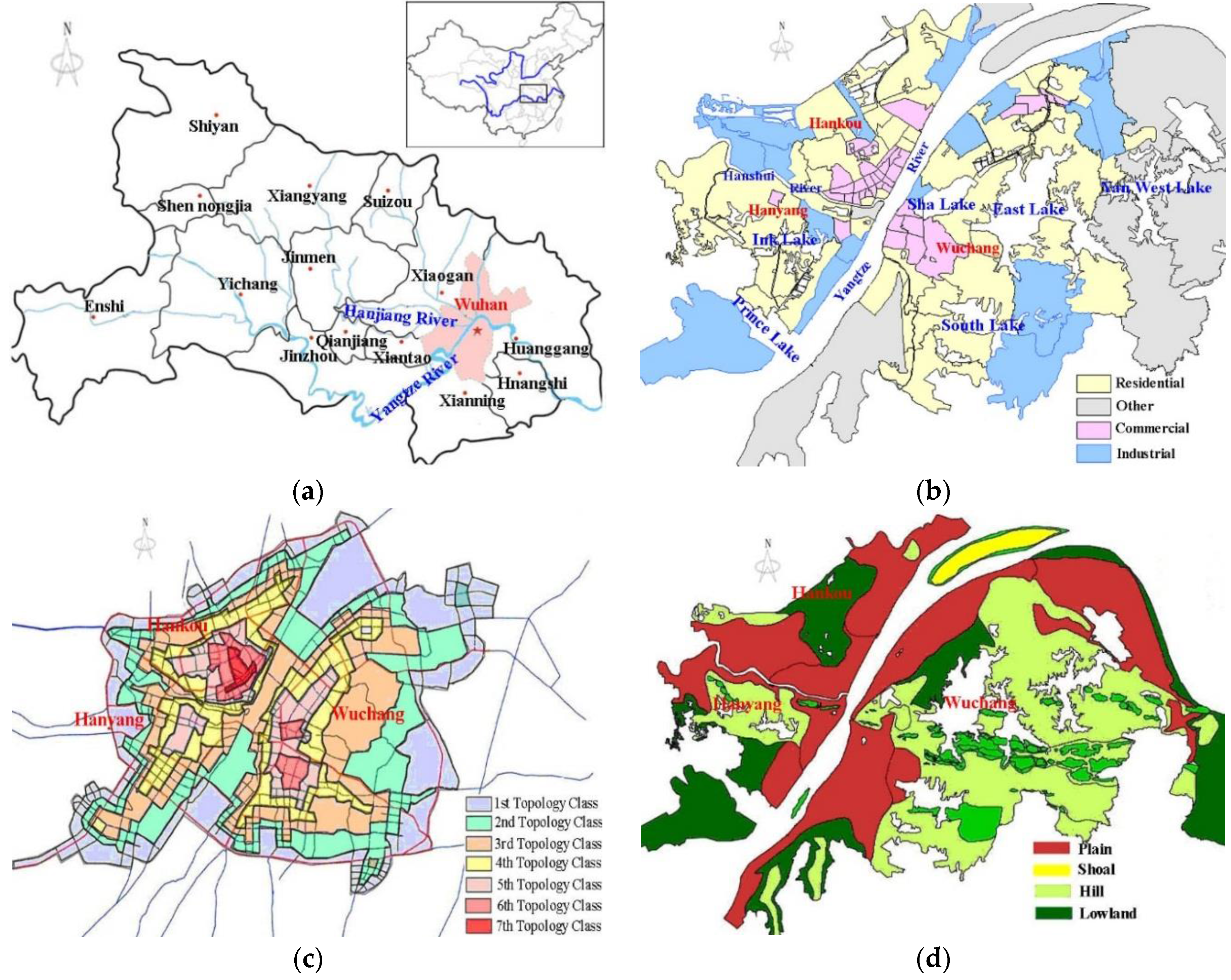
2.1. Study Area

Wuhan is located centrally in the People’s Republic of China, the biggest inland port city and the most important city in central China. Wuhan’s urban civilization dates back 3500 years to Panlong Town, which is the oldest city unearthed to date in the Yangtze River basin. As the capital of Hubei province, Wuhan serves as the political, economic and cultural center of the province. The Yangtze is the world’s third longest river, and its largest tributary, Hanjiang, meets it in Wuhan [58,59] (Figure 1a).

Yangtze and Hanjiang divide the city into the three parts of Hankou, Hanyang and Wuchang, namely the “three towns of Wuhan”. The three towns have different spatial characteristics and different developmental tendencies for historical reasons. Among them, Wuchang is a center for culture and education, and the residential land cover is widely distributed. Hankou is a commercial center and a commercial land cover concentrated distribution. Hanyang is an industrial center, and industrial land cover is distributed in the urban fringe. As a typical garden city featuring mountains and water, Wuhan is home to hundreds of hills and nearly 200 lakes of various sizes. With water comprising 25.8% of its area, Wuhan is ranked first among major Chinese cities in water resources [60] (Figure 1b).

As the largest water, land and air transportation hub in inland China, Wuhan is a major transportation hub, with dozens of railways, roads and expressways passing through the city. The road traffic networks in Wuhan are greatly affected by the Yangtze and Hanjiang, showing the multi-core concentrate networks mode. With the political, economic and commercial center as a core, the road traffic network’s density declines with spatial distance. The road network topological class is a layer-circle decreasing distribution [58] (Figure 1c).

Geographically, Wuhan is located between latitudes 29°58′N and 31°22′N and longitudes 113°41′E and 115°05′E. Topographically, Wuhan belongs to the transitional belt from the southeast highlands to foothills in the south piedmont of Dabie Mountain. The middle part is low and flat, and the south part and north part are hills. The landform types belong to an alluvial plain of rivers and lakes, with many lakes and rivers [4,15] (Figure 1d).

2.2. Data

The original data used in this paper are vector map data, raster map data and interrelated statistical data. The spatial attribute information of the study area, such as land cover type, road accessibility, topographic gradient, building density, etc., is interpreted from the vector and raster map by using ESRI’s ArcGIS 9.3 software (ESRI Corp. Redlands, CA, USA, 2013). The non-spatial data are also the foundation of spatial pattern analysis, which are processed and calculated by using Excel and VC++ from the interrelated statistical data, such as the Wuhan statistical yearbook. To reduce the computational complexity in the construction of the Voronoi diagram and the large-scale spatial data analysis, we select Hankou as the study area. Hankou has a land area of 139.57 km², with water accounting for approximately 4%.

3. Methodology

3.1. Voronoi Diagrams Used to Compare the Distance Extension

Voronoi diagrams and Delaunay triangulation are very important theoretical methods in computational geometry. The study of Voronoi diagrams can be traced back to the seminal work by Voronoi [49]. Consider some d-dimensional space in which a number of given points (sometimes referred to as seeds, attractors or generators) is located. To each seed, we assign a Voronoi set that includes all points that are closer to the seed to which it is assigned than to any other seed. The collection of all Voronoi sets is then a Voronoi diagram [61]. Voronoi diagrams are a very simple geometrical construct with numerous applications, such as biology, ecology, epidemiology, materials science, machine learning, geography and geology, because of the adjacency similarity and systematic theoretical system [62,63,64,65]. The Voronoi diagram is an important spatial interpolation method because of its geometric structure. Indeed, it can be used to determine the value of any unknown point based on the nearest known point’s value [66,67,68]. The concept of distance is central to Voronoi diagrams. While there are many types of distances, such as polyhedral distance, Gauges distance and Euclidean distance [61,69], we improve the distance by integrating the geospatial proximity distance and attribute similarity distance.

In this paper, the Voronoi diagrams’ character is used to construct a Voronoi diagram model for spatial pattern research based on the generalized Euclidean distance (integrating the geospatial proximity distance and the attribute similarity distance) of sampling point datasets. Then, the urban land use spatial clustering homogeneous segmentation of the study area is performed based on the sample data. The extended, weighted Voronoi diagrams can be described as follows:

We define the center point set as $P=\left\{p_1,p_2,p_i,\cdots ,p_n\right\}$, where $p_i$ is any given center point, $\left(x_i,y_i\right)$ is $p_i$’s spatial location and $A\left(p_i\right)=\left(a_{i1},a_{i2},\cdots ,a_{in}\right)$ expresses its attribute vector. In the conventional Voronoi diagram model, the comparison distance is the geometry distance in the Euclidean plane, and the effect of the attribute similarity distance is not considered. In this paper, the geospatial proximity distance is calculated by the following equation:

$$D_{Spat}\left(p_i,p_j\right)=w_x{\left(x_i-x_j\right)}^2+w_y{\left(y_i-y_j\right)}^2$$

(1)

In this paper, $D_{Attr}\left(p_i,p_j\right)$ is the attribute similarity distance between points $p_i$ and $p_j$ and is calculated by the following equation:

$$D_{Attr}\left(p_i,p_j\right)={\displaystyle \sum _{k=1}^m}{w}_k{\left(a_{ik}-a_{jk}\right)}^2$$

(2)

The geospatial proximity distance and attribute similarity distance are integrated to define the generalized Euclidean distance of the Voronoi diagrams as follows:

$$D_{ij}=\sqrt{D_{Spat}\left(p_i,p_j\right)+D_{Attr}\left(p_i,p_j\right)}$$

(3)

where $w_x,w_y$ are the weight coefficients of the spatial coordinates $x,y$ and $w_k$ is the weight coefficient of the k feature in the attribute feature sets.

In this paper, evaluation indices are established by principal component analysis by using SPSS Statistics 19 (IBM Corp. Armonk, NY, USA, 2010) [70]. The evaluation index system indicators include the residential floor area ratio (U1), building density (U2), population density (U3), green area (U4), road accessibility (U5), pipe network status (U6), healthcare (U7), universities and colleges (U8), stadium completion degree (U9), noise index (U10), land price (U11) and land idle rate (U12). In this paper, we index the data into point, line and polygon indices according to the respective influences on the spatial pattern base of the study area’s grid map.

• Point index (including the healthcare index, universities and college index and stadiums index): This index is calculated using the linear model based on the grid center. The basis of the service radius from the inside to the outside is used to calculate the attribute value according to the distance linear attenuation model:

  $$\begin{array}{ccc}{F}_i=f_0\left(1-r_i\right)& r_i=D_i/D_0& 0\le r_i\le 1\end{array}$$

  (4)

  where $F_i$ is the action mark of the index, $f_0$ is the comprehensive scale index of the numerical standardization involved in Geographic Information System (GIS) buffer analysis, $D_0$ is the maximum impacted distance of this index and $D_i$ is the geometric distance between this index and another spatial point.
• Line index (including road accessibility): This index is calculated using the exponential model along the linear target. The basis of the service radius from the inside to the outside is used to calculate the attribute value according to the distance decay exponential model:

  $$\begin{array}{ccc}{F}_i={f_0}^{\left(1-r_i\right)}& r_i=D_i/D_0& 0\le r_i\le 1\end{array}$$

  (5)
• Polygon index (including the noise index): This index is obtained by calculating the action mark directly.

  $$F_i=100\times \frac{X_i-X_{min}}{X_{max}-X_{min}}$$

  (6)

  where $F_i$ is the action mark of the index, $X_i$ is the evaluation value of the grid index and $X_{min}$ and $X_{max}$ are the minimum and maximum values of this index, respectively.

Index weights reflect the importance of each indicator in the index system, and they are often determined by, for example, the Delphi method or the Analytic Hierarchy Process (AHP) [71,72,73]. In this paper, we use AHP to obtain the weight for each index (

Table 1. Evaluation index weighting coefficient table.

Index	Weight	Index	Weight	Index	Weight
residential floor area ratio (U1)	0.1592	building density (U2)	0.1304	population density (U3)	0.1001
green area (U4)	0.1052	road accessibility (U5)	0.0706	pipe network status (U6)	0.0583
health care (U7)	0.0544	universities and colleges (U8)	0.0476	stadium completion degree (U9)	0.0424
noise index (U10)	0.0537	land price (U11)	0.0821	land idle rate (U12)	0.0960

).

3.2. Spatial Aggregation and Separation Index of Voronoi Diagrams

The Aggregation Index (AI) describes the randomness or aggregation degree of landscapes and was proposed by O’Neill in 1988 under the name ‘Contagion Index’ (CI) [74]. The aggregation index reflects the spatial configuration of landscape components [75,76]. Consequently, the land use type Voronoi polygonal neighborhood adjacent relationship is analyzed by calculating the Voronoi polygonal neighborhood aggregation index. Then, the overall spatial agglomeration and dispersion degree of land use are investigated.

• The Voronoi polygon self-neighborhood aggregation index is calculated with the following equation:

  $$\begin{array}{ccc}{\alpha }_{ik}=\left({\beta }_{ik}·x_{ik}\right)/n_i& & iϵN_k\end{array}$$

  (7)

  where $x_{ik}$ is one Voronoi polygon; ${\beta }_{ik}$ is the number of polygons whose land use type is k in the Voronoi polygon neighborhood; $n_i$ is the direct neighborhood polygon number of polygon $x_{ik}$ , which is obtained by recording the Voronoi vertex topology; and $N_k$ is the number of Voronoi polygons whose land use type is k.
• The Voronoi polygon regional aggregation index is calculated as follows:

  $${\delta }_k=\left({\displaystyle \sum _{i=1}^{N_k}}{\alpha }_{ik}·x_{ik}\right)/N_k$$

  (8)

  where ${\delta }_k$ is the sum of ${\alpha }_{ik}$ and ${\alpha }_{ik}$ is the Voronoi polygon self-neighborhood aggregation index obtained using Equation (7). ${\delta }_k$ is used to standardize the treatment: as ${\delta }_k\to 0$, the land use spatial distribution becomes more dispersed, whereas as ${\delta }_k\to 1$, the land use spatial distribution tends to coalesce.

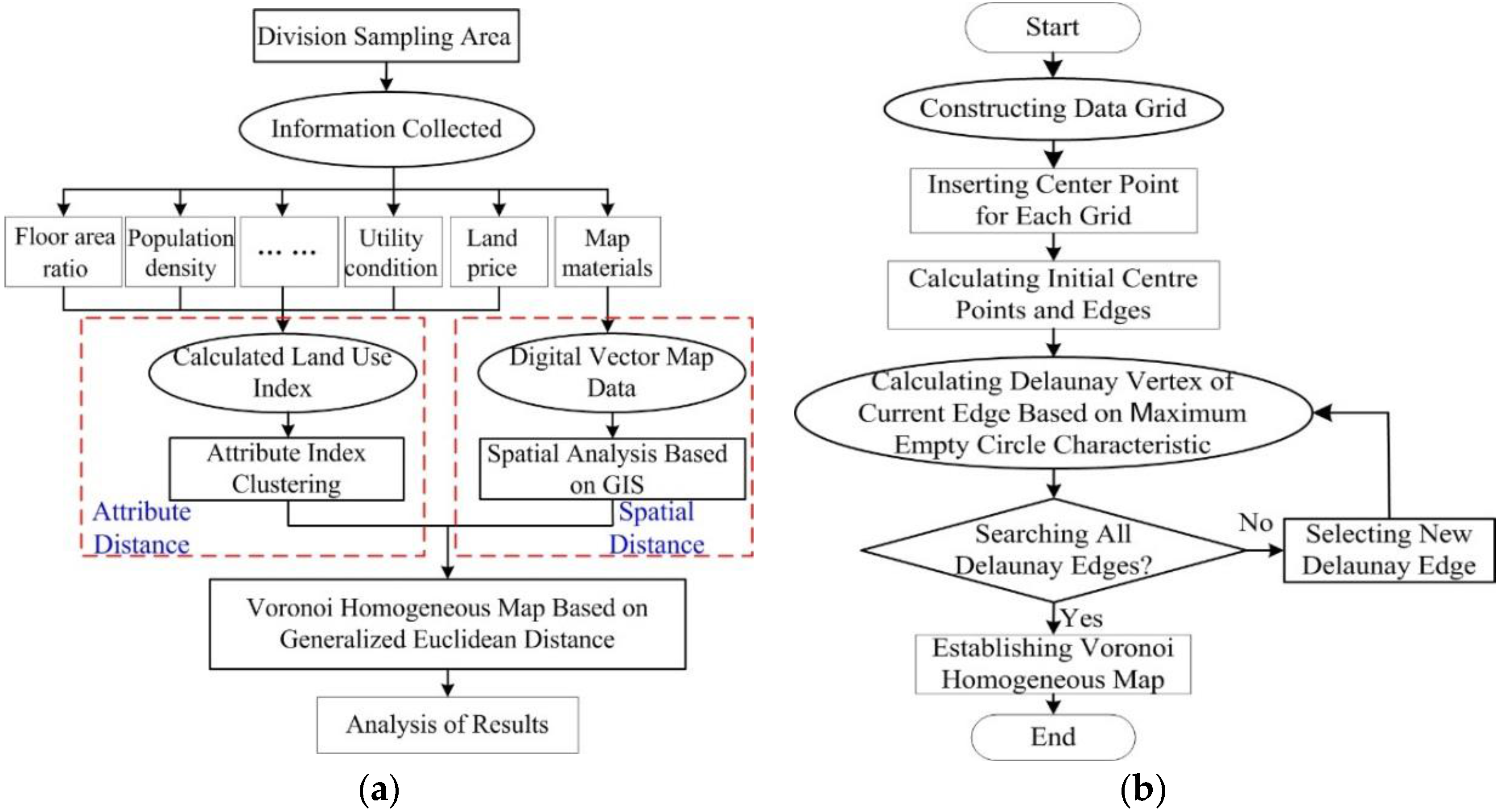
3.3. Technical Research Flowcharts

The technical research flowchart and main technical processes are presented in Figure 2.

• Step 1: The study map is divided into 100 m × 100 m grids by using ESRI’s ArcGIS 9.3 software.
• Step 2: A Voronoi diagram based on the center point dataset of sample points is constructed. Then, spatial overlay analysis between the Voronoi diagram and the current land use map is performed to obtain the land use type area for every Voronoi polygon. The spatial and attribute character parameters are saved into a spatial and attribute data table (

  Table 2. Land use grid spatial and attribute structures.

  No.	Field	Type	No.	Field	Type	No.	Field	Type
  1	Voronoi ID	Long	4	Vertex Datasets	CArray	7	Area	Float
  2	Coordinate	TPoint	5	Edge Datasets	CArray	8	Aggregation Index	Float
  3	Triangle ID	CList	6	Land Use Type	Int	9	Clustering level	Int

  ). In Table 2, the coordinate is the Voronoi polygon center point, and the triangle ID is the serial number of the Voronoi polygon Delaunay triangle. The vertex and edge datasets represent the vertex and edge of every Voronoi polygon. The land use type reflects the status of each land use type, such as 0, 1 and 2. Aggregation index and clustering level data are obtained in Step 3.
• Step 3: The model is used to calculate the neighborhood aggregation index for every Voronoi polygon using Equations (7) and (8). To obtain the clustering grade data, the model performs a cluster analysis based on the shortest distance method using SPSS software. Finally, the model produces the experimental Voronoi diagram map based on the principle of “similar category incorporation and heterogeneous merging”.

3.4. Voronoi Diagrams’ Building Process

In this paper, the sample datasets are used as the central point of the Voronoi diagrams. This novel model constructs Voronoi polygons by the Delaunay triangulation method based on the grid growth algorithm [77,78]. The main algorithm is built with the C# programming language based on the ArcGIS Engine and Visual Studio 2010 platform. The experimental process is shown in Figure 2b. The novel model defined the following data types for experimental program development: TPointSetArry as the center point set array, TPointsetList as the point set list, TriSetList as the edge set list, nTriCount as the number of Delaunay triangles and TPointSetListD as the Delaunay triangulation point set list.

3.4.1. Calculating the Initial Centre Points and Edges

• Step 1: Although any point can be used as the initial point P1, to improve program efficiency, a point near the center of the study area was chosen as the initial point of the grid. The numbers of initial center points and edges are stored in TPointSetArry and TPointSetList, respectively.
• Step 2: The model comparison distance is defined by Equation (3).
• Step 3: The initial value of $D_{min}$ is defined as the larger value. In this paper, the diagonal length of the graphic in the entire study area is defined as the initial value of $D_{min}$.
• Step 4: The distance between two points is calculated by using Equation (9) if the grid cell of the initial point also contains other points. This distance is then compared to $D_{min}$ to identify the nearest point to the initial point $P_1$. Selecting a small value reassigns it to $D_{min}$.
• Step 5: The adjacent grid cells are searched until the shortest side of $D_{min}$ is found, and the search pattern moves from left to right and from top to bottom. Then, the shortest side is taken as the initial Delaunay edge. The number of initial Delaunay edges is stored in TriSetList.

3.4.2. Constructing the Delaunay Triangulation

• Step 1: Taking $P_i{P}_j$ as the current processing edge, the intersect calculation is then performed with the bottom line of the grid cells to obtain the value of $i_1$. The intersection grid column gives the value of $j_1$. Similarly, the intersect calculation is conducted with the right bottom line of the grid cells to obtain the value of $j_2$. The intersection grid column provides the value of $i_2$. Finally, the cells $\left(i_1,j_1\right)$ and $\left(i_2,j_2\right)$ are obtained at the right grid.
• Step 2: The unit triangle is formed by three vertices: $\left(i_1,j_1\right)$, $\left(i_1,j_2\right)$ and $\left(i_2,j_2\right)$. The triangle circumcircle is then constructed.
• Step 3: Repeat Step 1 in the area covered by the circumcircle. The point that creates the largest angle with the current edge $P_i{P}_j$ is selected as the vertex. Then, the triangle is constructed in the circle formed by the points by repeating the previous steps until all of the grid units covered by the circumcircle are searched and no other vertex is available. The resulting triangle is a Delaunay triangle.
• Step 4: The center point and Delaunay triangle are numbered. The numbers of the three central points (vertices) that comprise the Delaunay triangle are recorded. These data are stored in TPointSetListD, and the numerical value of nTriCount is incremented by 1.

3.4.3. Constructing the Voronoi Homogeneous Diagram Map

• Step 1: As reported previously [79,80], all Delaunay triangle numbers adjacent to each center point are recorded and sorted in the anticlockwise direction.
• Step 2: A convex hull boundary with the peripheral boundary connects each center point of the adjacent triangles in the circumcircle. The entire experimental data area is searched using the novel model, and then, the Voronoi homogeneous diagram map of the study area is produce.

3.5. Spatial Clustering and Autocorrelation Analysis Method

The authors perform a clustering analysis of the Voronoi polygonal neighborhood aggregation index of the study area using SPSS software [70,81]. The clustering analysis applies the shortest distance method and the correlation coefficient as the cluster sign. The mutation of the correlation coefficient is the end mark of the cluster, and the absolute distance threshold is defined as 0.09.

Spatial autocorrelation (also known as spatial dependence, spatial interaction or local interaction) can be loosely defined as a similarity (or dissimilarity) measure between two values of an attribute that are nearby spatially [54]. Spatial autocorrelation can be measured by various indexes, of which probably the most well-known is Moran’s I statistic. Statistics like the global Moran’s I are useful for analyzing datasets in a relatively homogeneous region; it may not be as informative to compute the Moran’s I value for data across a region that could have several spatial regimes [55,82]. One solution is to develop a set of Local Indicators of Spatial Association (LISA), such as the local Moran’s I [55,82]. Therefore, we calculate the local Moran’s I data in the study area by using the spatial autocorrelation analysis (univariate Moran) function of the GeoDA software [83,84]. The generalized form for the local Moran’s I can be defined as follows [55]:

$$I_i\left(d\right)=Z_i{\displaystyle \sum _{j\ne i}^n}{W}_{ij}{Z}_j$$

(9)

where the observations $Z_i$ and $Z_j$ are in standardized form (with a mean of zero and a variance of one). The spatial weight $W_{ij}$ is in row-standardized form. Therefore, $I_i$ is a product of $Z_i$ and the average of the observations in the surrounding locations.

The Moran scatter plot visually illustrates the spatial transformation of a variable (y-axis) on the original standardized variable (x-axis). The slope of the scatter plot corresponds to the value for Moran’s I. According to the Moran scatter plot, we can find the extent of linear association between the values in a given location (x-axis) with the values of the same variable in neighboring locations (y-axis) [82,85].

4. Results and Discussion

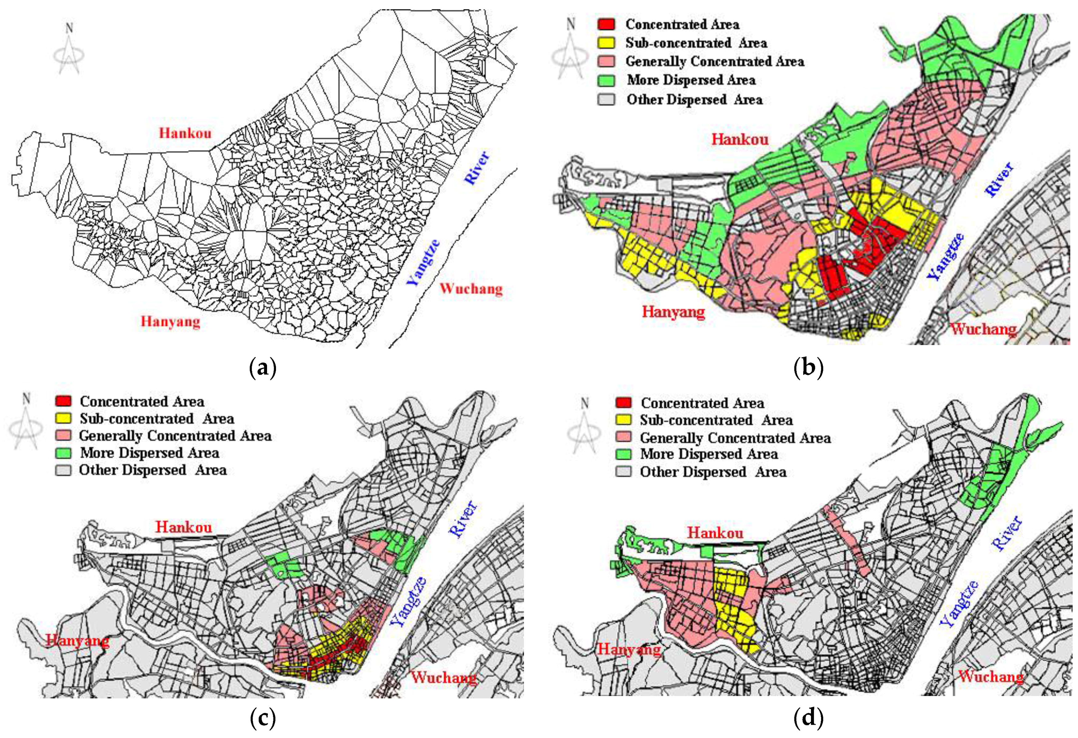
4.1. Spatial Pattern Clustering Results

The clustering analysis results and frequency histogram are shown as

Table 3. Statistical analysis of the Voronoi polygon aggregation index for each land use type.

Level	Residential Land			Commercial Land			Industrial Land
	Index Value	Area (hm2)	Ratio (%)	Index Value	Area (hm2)	Ratio (%)	Index Value	Area (hm2)	Ratio (%)
1st level	≥0.83	16.58	12.52	≥0.89	3.28	13.94	0.00	0.00	0.00
2nd level	0.75~0.82	27.32	20.63	0.77~0.88	6.57	27.92	0.69~0.78	8.49	18.39
3rd level	0.49~0.74	47.60	35.94	0.52~0.76	8.59	36.49	0.42~0.68	24.40	52.86
4th level	0.33~0.48	40.94	30.91	0.38~0.51	5.10	21.65	0.29~0.41	13.27	28.75

and Figure 3, respectively. In Figure 3, the horizontal coordinate is the value of each land aggregation index, and the vertical coordinate is the ratio of each land use frequency to the group distance.

We merge Voronoi polygons according to the cluster level, merge smaller polygons based on the principle of the longest shared boundary and then obtain the spatial agglomeration pattern Voronoi homogeneous map of the study area (Figure 4a).

Clustering results of residential land use: The concentrated clustering classification land use area (first level) accounts for 12.52% of the total area and is mainly located along Jiefang road, Hangkong road, Baofeng road and Huangpu road, where municipal establishments are complete and transportation is convenient. The sub-concentrated clustering classification land use area (second level) accounts for 20.63% of the total area and is primarily found along Fazhan road, where new contiguous residential areas, building density and building volume rates are higher. The generally concentrated clustering classification land use area (third level) accounts for 35.94% of the total area, is mainly located in Changfeng township and mostly consisted of urban peripheries, where the layout is not complete and the environment is general. The dispersed clustering classification land use area (fourth level) accounts for 30.91% of the total area and is primarily noted along Houhu road, where the building density and building floor area ratio is low, the building distribution is dispersive, the municipal establishments are not complete and the environment is poor.

Clustering results of commercial land use: The concentrated clustering classification land use area (first level) accounts for 13.94% of the total area and is mainly located in the street business district on both sides of Zhongshan avenue, where abundant, densely-packed financial, insurance and high-rise office buildings, luxury hotels and passenger flow are located. The sub-concentrated clustering classification land use area (second level) accounts for 27.92% of the total area and is typically located in the peripheral zone of Zhongshan avenue, hosting regional traffic, a high building density and construction volume and completed municipal facilities, which attract a large passenger flow. The generally concentrated clustering classification land use area (third level) accounts for 36.49% of the total area, primarily along Baofeng road, North lake road, Station road and Huangpu road. In these areas, the facilities are complete, and the layout of the environment is mixed use. The greatest potential of these regions is for mining because of the rapid economic development and the improvement of infrastructure. The dispersed clustering classification land use area (fourth level) accounts for 21.65% of the total area and is mainly comprised of the Hankou railway station and Huangpu Avenue East theatre. The commercial network density is relatively low, and the passenger flow is not significant, mainly corresponding to regional business services. These regions have the additional advantages of comprehensive exploitation and application.

Clustering results of industrial land use: The generally concentrated clustering classification land use area (third level) and the dispersed clustering classification land use area (fourth level) account for 81.61% of the total industrial land use area. The industrial lands are mainly located in the city’s peripheral area, such as Chanfeng road, where the Qiaokou economic and technological development zone is. Additionally, it is mainly located in north Hankou districts, containing the Panlong economic and technological development zone and the north Hankou metropolitan industrial park. The average efficiency of the industrial land is low because the government restricts industrial areas in cities to improve the urban environment and the economic, social and ecological benefits of urban land use. The area of industrial land declined under the policy of “industrial factory relocation from the second ring zone and replacement with green plants”.

Spatial autocorrelation results: The Moran scatter plot in Figure 5 illustrates the relationship between each spatial clustering patch. In which, the horizontal coordinate is the standard value of each unit’s intensive degree and the vertical coordinate is the average value of the properties of neighboring units. In the Moran scatter plot, the slope of the regression line corresponds to Moran’s I; the four quadrants of the coordinate system correspond to the four types of local space between the regional unit and its neighbors.

The slope of the regression line in the Moran scatter plot is 0.0537, which represents the residential land cover present spatial positive correlation (Figure 5a). The Moran scatter plots are mainly distributed in the first, second and third quadrant, belong to high-high, low–high and low–low spatial clustering. For the Moran scatter plot, the first quadrant of the coordinate system represents the spatial connectivity of the high observed value area unit surrounded by the high observed value region (high–high); the second quadrant of the coordinate system represents the spatial connectivity of the low observed value area units surrounded by the high observed value region (low–high); and the third quadrant of the coordinate system represents the spatial connectivity of the low observed value area unit surrounded by the low observed value region (low-low) [83]. The high–high clustering units in the first quadrant are few compared to the low-low and low-high clustering units in the second and third quadrants. Therefore, the aggregation advantage of residential land use in the study area has an accumulative effect, but the aggregation advantage is not significant and the spatial difference between the overall levels of stacking utilization not large. In Figure 4b, the high–high clustering areas of residential land cover are mainly located in Jiefang road, Hangkong road, Fazhan road, Laodong road, Yongqing road and Wansong road, which are adjacent to the commercial districts, with perfect facilities and convenient traffic; the spatial clustering classes are mainly including the first and second level. The low–high clustering areas are widely distributed in the study area, showing the spatial dispersion characteristics and the spatial clustering class at the third level. Low–low clustering areas are mainly located in urban fringes; the spatial clustering class is the fourth level.

The slope of the regression line in the Moran scatter plot is 0.1658, which represents that the commercial land cover aggregation presents considerable spatial autocorrelation (Figure 5b). The Moran’s I of commercial land is maximized. The maximum value of the gradient of the intensive degree value indicates that the spatial agglomeration of commercial land is considerable compared to those of other land uses and is subject to a spatial agglomeration effect. The Moran scatter plots are mainly distributed in the first and third quadrant, belong to high–high and low–low spatial clustering. The high–high clustering units in the first quadrant are large compared to the low–low clustering units in the third quadrant. Therefore, the commercial land use in the study area has high utilization efficiency and a high intensive utilization degree. In Figure 4c, the high–high clustering areas of commercial land cover are mainly located in the street business districts along Zhongshan Avenue on both sides, with extremely dense commercial networks and extremely high land use efficiency and intensive degree; the spatial clustering classes mainly include the first, second and third level. The low–low clustering areas are mainly located in Hankou railway station with low density commercial networks; the spatial clustering class is the fourth level. The spatial difference of commercial network density in other regions is obvious and shows dispersion characteristics.

The slope of the regression line in the Moran scatter plot is 0.1473, which represents that the industrial land cover presents a spatial positive correlation (Figure 5c). The Moran scatter plots are mainly distributed in the first and third quadrant, belonging to high–high and low–low spatial clustering. The high–high clustering units in the first quadrant are few compared to the low–low clustering units in the third quadrant. Therefore, the industrial land use in the study area has increased utilization efficiency. The Moran’s I of industrial land is compared to those of other types of land use. The degree of spatial agglomeration is greater than that of residential land and less than that of commercial land. Additionally, this value responds to the actual situation of industrial land, which is mainly distributed in several development zones. In Figure 4d, the high–high clustering areas of industrial land use are mainly located on Chanfeng road, which is the Qiaokou economic and technological development zone; the spatial clustering classes mainly include the first and second level. The low–low clustering areas are mainly locate in the north Hankou districts, which contain the Panlong economic and technological development zone; the spatial clustering class is the fourth level.

4.2. Discussion

An urban area is not just a single agglomeration of people in space, but rather consists of numerous large and small clusters of households, firms and infrastructures that exhibit spatial patchiness in their social and economic structures [86]. The spatial structure and temporal dynamics of urban areas are complex and controlled by various driving forces, such as the regional economy, population movements, the policy environment and socio-cultural processes [87].

According to neo-Marxist theory, conventional urban science explains the urban phenomena partially with the factors of technology and population migrations, which are considered as principal causes of urban structural change [88]. In a neo-Marxist analysis, however, these are not the underlying causes, but instead are intermediate factors produced by something more fundamental, such as the basic requirements and social relations of capitalist production. Neo-Marxists present the structure of urban structure and land use/cover as the result of capitalism in pursuit of profit [88,89,90]. “Since the process of capital accumulation unfolds in a spatially structured environment, urbanism may be viewed provisionally as the particular geographical form and spatial patterning of relationships taken by the process of capital accumulation” [54,90].

Through different prices of land rent, land tax theory determines the spatial distribution of land use. According to the bidding land tax curve model, the land tax of commercial, residential and industrial land use is negatively related to the distance from the city center. Under the equilibrium condition of land tax and distance, the commercial land should be arranged in the nearest place from the city center, then residential land, and the farthest is the industrial land. In a spatial pattern, the concentric circle layer structure is distributed around the city center [91]. In the study area, the price of land tax is decreasing from the city center to the periphery. In Figure 4c and Figure 6a, a high density commercial district is mainly located in the first grade land tax area, which is the oldest and largest commercial district at present. Residential location patterns are characterized by significant spatial interrelationships across race, income, neighborhood quality, traffic accessibility and distance from a functional area (such as shopping malls, schools, hospitals, parks, etc.) [87]. No matter how large the scale of the functional area is, the spatial diffusion range is limited and close to the functional area to become the first choice for residential land. In Figure 4b and Figure 6a, most residential land is located in the second and third grade land tax area, a contiguity commercial district. Industrial land use is located in the urban fringe, where land resources and labor resources are rich, and it provides convenience for industrial organization, layout and optimization. In sum, the influence of land tax theory on the urban spatial structure of the study area is very obvious, and the urban spatial structure is characterized by a concentric layer structure from the urban center to the urban fringe. The urban spatial structure will transfer from a single center structure to a multi-center decentralized structure.

The government’s macro control policies have affected the urban spatial structure. In the study area, “industry quits from the second ring zone and enters into the third ring zone” is the urban management policy to adjust the industrial structure. The formation of the Qiaokou economic and technological development zone, which is located in the urban fringe, stimulated the construction of the surrounding facilities. With the gradual improvement of living facilities, commercial facilities and the transportation network, the surrounding real estate industry has been stimulated. The new center of the city has been developing and growing, which will eventually develop into a sub-center of the city.

Though land tax is believed to be the primary cause for shaping the urban spatial structure in the study area, other causes, such as population growth, economic investment and development, need to be examined. In Figure 6b, the permanent residents increase slowly with an annual average growth under 1%. The reason is that the study area was an old urban district, and the number of permanent residents tends to be saturated. However, in China, the difference of the urban and rural economic structure causes the income difference between urban and rural areas, and a large number of floating population migrates into cities, as commerce cluster areas can provide them considerable employment opportunities. In response, the floating population promotes a further agglomeration in this area.

At the same time, with an increase of the income, the level of residents’ consumption and demand improving gradually, the demand on the living environment, scale and level of commercial facilities continues to improve. Since the 1990s, China has implemented a series of land system reform policies including “an auction way to implement the transfer of land-use right” and “abolishing the welfare housing system”. Along with the housing commercialization carried out in China, more and more urban residents begin to escape from the “unit community” and purchase marketable housing based on their own abilities and preferences. The real estate industry has made outstanding contributions to the urban economy development, and the growing investment in real estate development has driven the synchronous development of the urban spatial structure agglomeration at the same time. For example, in 2009, Hankou’s investment in real estate development was 23.05 billion RMB with an increase rate of 59.44% over 2008, and the annual per capita disposable income of urban residents was 18,663 RMB with an increase rate of 15.60% over 2008. For the corresponding period, the area of commercialized housing sold was 2.84 million m² with an increase rate of 71.83% over 2008. The correlation between urban structure aggregation and disposable income of urban residents/investment on real estate development was examined, and it reveals a very strong association (Figure 6b).

5. Conclusions and Future Work

Wuhan is now at a stage of rapid urbanization, and urban studies are needed for a better understanding of the urban growth mechanism, to support land use planning for sustainable urban land use and protection. The spatial pattern of urban land use is affected by a series of factors, including both spatial factors (spatial relationships) and non-spatial factors (attribute relationships), such as political and economic factors. This research focuses on how to use modern theory and technology to describe these factors reasonably, to obtain results that reflect reality and to avoid separating theory from practice.

In this paper, a spatial agglomeration analysis of urban land use based on spatial adjacency and similar attribute characteristics is performed. To this end, the spatial and attribute characteristics are integrated into the generalized Euclidean distance to extend the traditional Voronoi diagram. This novel model constructs a Voronoi homogeneous map based on sample point datasets and the spatial attribute generalized Euclidean comparison distance. The spatial neighborhood aggregation indexes of the Voronoi polygons in the study area are calculated based on landscape ecology theory. The model generated the spatial Voronoi homogeneous map based on the spatial clustering grade of the neighborhood clustering indexes using SPSS software. In addition, the spatial autocorrelation of the urban spatial structure in the study area is analyzed by calculating the local Moran’s I using the GeoDA software.

Although population growth triggered by rural-urban migration generally was believed to be the dominant cause for urban spatial structure changes [7], according to the neo-Marxist theory, we briefly analyze the driving forces for shaping the urban spatial structure, and the analysis indicates that the different price of land rent, the government’s macro control policies and investment in real estate development are the major factors for the rapid urban spatial structure changes in the study area. The present study is expected to have significant implications in rapidly urbanizing cities of this developing country.

This research is only one example of using extended Voronoi diagrams to study the urban spatial pattern, and as such, this is a prototype. There is still much potential for developing this research further. Future research will focus on using the self-organizing theory of neural networks to cluster the classifications of attribute information, using a gravity model to improve the quantitative expression of physical space and attribute correlation [92]. The four forks tree method will be used to study the spatial data structure, and the efficiency of spatial data insertion and queries for improving the triangular surface construction in Voronoi diagrams will be evaluated. In addition, the self-organizing maps (SOM) may have a profound and significant role in merging decision makers based on multi-dimensional spatial data analysis [92,93]. The complexity of human movements has redefined the usage of urban space and the arrangement of resources; changes in the lifestyles of urban residents have prominent and visible effects on urban spatial metrics [92]. Most of these changes have been brought by human impact on the environment and excessive exploitation of resources. In this sense, the urban spatial patterning research approach should be “intelligent” and yield important insights into urban phenomena generated by human movements (social, natural and economic) [9].

References

1. Dewan, A.M.; Corner, R.J. Spatiotemporal analysis of urban growth, sprawl and structure. In Dhaka Megacity: Geospatial Perspectives on Urbanisation, Environment and Health; Dewan, A., Corner, R., Eds.; Springer: Dordrecht, The Netherlands, 2014; pp. 99–121. [Google Scholar]
2. Tewolde, M.G.; Cabral, P. Urban sprawl analysis and modeling in asmara, eritrea. Remote Sens. 2011, 3, 2148–2165. [Google Scholar] [CrossRef]
3. Rahman, M. Detection of land use/land cover changes and urban sprawl in al-khobar, saudi arabia: An analysis of multi-temporal remote sensing data. ISPRS Int. J. Geo-Inf. 2016, 5, 15. [Google Scholar] [CrossRef]
4. Wang, X.; Ning, L.; Yu, J.; Xiao, R.; Li, T. Changes of urban wetland landscape pattern and impacts of urbanization on wetland in wuhan city. Chin. Geogr. Sci. 2008, 18, 47–53. [Google Scholar] [CrossRef]
5. Dewan, A.M.; Yamaguchi, Y. Land use and land cover change in greater dhaka, bangladesh: Using remote sensing to promote sustainable urbanization. Appl. Geogr. 2009, 29, 390–401. [Google Scholar] [CrossRef]
6. Dewan, A.M.; Yamaguchi, Y. Using remote sensing and gis to detect and monitor land use and land cover change in dhaka metropolitan of bangladesh during 1960–2005. Environ. Monit. Assess. 2008, 150, 237–249. [Google Scholar] [CrossRef] [PubMed]
7. Dewan, A.M.; Yamaguchi, Y.; Ziaur Rahman, M. Dynamics of land use/cover changes and the analysis of landscape fragmentation in dhaka metropolitan, bangladesh. GeoJ 2012, 77, 315–330. [Google Scholar] [CrossRef]
8. Irwin, E.G. New directions for urban economic models of land use change: Incorporating spatial dynamics and heterogeneity. J. Reg. Sci. 2010, 50, 65–91. [Google Scholar] [CrossRef]
9. Vaz, E. The future of landscapes and habitats: The regional science contribution to the understanding of geographical space. Habitat Int. 2016, 51, 70–78. [Google Scholar] [CrossRef]
10. Nijkamp, P.; Kourtit, K. The “new urban europe”: Global challenges and local responses in the urban century. Eur. Plan. Stud. 2013, 21, 291–315. [Google Scholar] [CrossRef]
11. Byomkesh, T.; Nakagoshi, N.; Dewan, A.M. Urbanization and green space dynamics in greater dhaka, bangladesh. Landsc. Ecol. Eng. 2012, 8, 45–58. [Google Scholar] [CrossRef]
12. Gordon, A.; Simondson, D.; White, M.; Moilanen, A.; Bekessy, S.A. Integrating conservation planning and landuse planning in urban landscapes. Landsc. Urban Plan. 2009, 91, 183–194. [Google Scholar] [CrossRef]
13. Sakieh, Y.; Salmanmahiny, A.; Jafarnezhad, J.; Mehri, A.; Kamyab, H.; Galdavi, S. Evaluating the strategy of decentralized urban land-use planning in a developing region. Land Use Policy 2015, 48, 534–551. [Google Scholar] [CrossRef]
14. Rodrigue, J.P. Geography of Transport Systems, 3rd ed.; Routledge, Taylor & Francis Group: New York, NY, USA, 2013. [Google Scholar]
15. Zeng, C.; Liu, Y.; Stein, A.; Jiao, L. Characterization and spatial modeling of urban sprawl in the wuhan metropolitan area, China. Int. J. Appl. Earth Observ. Geoinf. 2015, 34, 10–24. [Google Scholar] [CrossRef]
16. Xiao, J.; Shen, Y.; Ge, J.; Tateishi, R.; Tang, C.; Liang, Y.; Huang, Z. Evaluating urban expansion and land use change in shijiazhuang, china, by using gis and remote sensing. Landsc. Urban Plan. 2006, 75, 69–80. [Google Scholar] [CrossRef]
17. Ma, Y.; Xu, R. Remote sensing monitoring and driving force analysis of urban expansion in guangzhou city, china. Habitat Int. 2010, 34, 228–235. [Google Scholar] [CrossRef]
18. Hsu, W.-T. Central place theory and city size distribution*. Econ. J. 2012, 122, 903–932. [Google Scholar] [CrossRef]
19. Abdel-Rahman, H.M.; Wang, P. Toward a general-equilibrium theory of a core-periphery system of cities. Reg. Sci. Urban Econ. 1995, 25, 529–546. [Google Scholar] [CrossRef]
20. Kuby, M. A location-allocation model of lösch’s central place theory: Testing on a uniform lattice network. Geogr. Anal. 1989, 21, 316–337. [Google Scholar] [CrossRef]
21. Thomas, M.D. Growth pole theory, technological change, and regional economic growth. Pap. Reg. Sci. 1975, 34, 3–25. [Google Scholar] [CrossRef]
22. Mansury, Y.; Gulyás, L. The emergence of zipf’s law in a system of cities: An agent-based simulation approach. J. Econ. Dyn. Control 2007, 31, 2438–2460. [Google Scholar] [CrossRef]
23. Baynes, T.; Heckbert, S. Micro-scale simulation of the macro urban form: Opportunities for exploring urban change and adaptation. In Multi-Agent-Based Simulation X, Proceedings of International Workshop MABS 2009, Budapest, Hungary, 11–12 May 2009; pp. 14–24.
24. Chen, Y.; Zhou, Y. Scaling laws and indications of self-organized criticality in urban systems. Chaos Solitons Fractals 2008, 35, 85–98. [Google Scholar] [CrossRef]
25. Batty, M. Complex spatial systems: The modelling foundations of urban and regional analysis. Urban Stud. 2001, 38, 1402–1404. [Google Scholar]
26. Amson, J.C. Catastrophe theory: A contribution to the study of urban systems? Environ. Plan. B Plan. Des. 1975, 2, 177–221. [Google Scholar] [CrossRef]
27. Batty, M. Cities and fractals: Simulating growth and form. In Fractals and Chaos; Springer-Verlag New York, Inc.: New York, NY, USA, 1991; pp. 43–69. [Google Scholar]
28. Wong, D.W.S.; Fotheringham, A.S. Urban systems as examples of bounded chaos: Exploring the relationship between fractal dimension, rank-size, and rural-to-urban migration. Geogr. Ann. 1990, 72, 89–99. [Google Scholar] [CrossRef]
29. Portugali, J. Self-organization and the city. In Encyclopedia of Complexity and Systems Science; Meyers, A.R., Ed.; Springer New York: New York, NY, USA, 2009; pp. 7953–7991. [Google Scholar]
30. Yeh, A.G.O.; Li, X. Measurement and monitoring of urban sprawl in a rapidly growing region using entropy. Photogramm. Eng. Remote Sens. 2001, 67, 83–90. [Google Scholar]
31. Aguilera, F.; Valenzuela, L.M.; Botequilha-Leitão, A. Landscape metrics in the analysis of urban land use patterns: A case study in a spanish metropolitan area. Landsc. Urban Plan. 2011, 99, 226–238. [Google Scholar] [CrossRef]
32. Black, D.; Henderson, V. A theory of urban growth. J. Political Econ. 1999, 107, 252–284. [Google Scholar] [CrossRef]
33. Eaton, J.; Eckstein, Z. Cities and growth: Theory and evidence from france and japan. Reg. Sci. Urban Econ. 1997, 27, 443–474. [Google Scholar] [CrossRef]
34. Sklar, F.H.; Costanza, R. The development of dynamic spatial models for landscape ecology: A review and prognosis. Ecol. Stud. Anal. Synth. 1991, 82, 239–288. [Google Scholar]
35. Parker, D.C.; Manson, S.M.; Janssen, M.A.; Hoffmann, M.J.; Deadman, P. Multi-agent systems for the simulation of land-use and land-cover change: A review. Ann. Assoc. Am. Geogr. 2003, 93, 314–337. [Google Scholar] [CrossRef]
36. Araya, Y.H.; Cabral, P. Analysis and modeling of urban land cover change in Setúbal and Sesimbra, portugal. Remote Sens. 2010. [Google Scholar] [CrossRef]
37. Herold, M.; Goldstein, N.C.; Clarke, K.C. The spatiotemporal form of urban growth: Measurement, analysis and modeling. Remote Sens. Environ. 2003, 86, 286–302. [Google Scholar] [CrossRef]
38. Cromley, G.R.; Hanink, M.D. Coupling land use allocation models with raster gis. J. Geogr. Syst. 1999, 1, 137–153. [Google Scholar] [CrossRef]
39. Chen, Y.; Li, X.; Liu, X.; Ai, B.; Li, S. Capturing the varying effects of driving forces over time for the simulation of urban growth by using survival analysis and cellular automata. Landsc. Urban Plan. 2016, 152, 59–71. [Google Scholar] [CrossRef]
40. Nourqolipour, R.; Shariff, A.R.B.M.; Ahmad, N.B.; Balasundram, S.K.; Sood, A.M.; Buyong, T.; Amiri, F. Multi-objective-based modeling for land use change analysis in the south west of selangor, malaysia. Environ. Earth Sci. 2015, 74, 4133–4143. [Google Scholar] [CrossRef]
41. Almeida, C.M.; Gleriani, J.M.; Castejon, E.F.; Soares, B.S. Using neural networks and cellular automata for modelling intra-urban land-use dynamics. Int. J. Geogr. Inf. Sci. 2008, 22, 943–963. [Google Scholar] [CrossRef]
42. Wang, F.; Marceau, D.J. A patch-based cellular automaton for simulating land-use changes at fine spatial resolution. Trans. GIS 2013, 17, 828–846. [Google Scholar] [CrossRef]
43. Barreira-González, P.; Gómez-Delgado, M.; Aguilera-Benavente, F. From raster to vector cellular automata models: A new approach to simulate urban growth with the help of graph theory. Comput. Environ. Urban Syst. 2015, 54, 119–131. [Google Scholar] [CrossRef]
44. Moreno, N.; Wang, F.; Marceau, D.J. Implementation of a dynamic neighborhood in a land-use vector-based cellular automata model. Comput. Environ. Urban Syst. 2009, 33, 44–54. [Google Scholar] [CrossRef]
45. Páez, A.; Scott, D.M. Spatial statistics for urban analysis: A review of techniques with examples. GeoJ 2005, 61, 53–67. [Google Scholar] [CrossRef]
46. Luck, M.; Wu, J. A gradient analysis of urban landscape pattern: A case study from the phoenix metropolitan region, arizona, USA. Landsc. Ecol. 2002, 17, 327–339. [Google Scholar]
47. Getis, A.; Ord, J.K. The analysis of spatial association by use of distance statistics. In Perspectives on Spatial Data Analysis; Anselin, L., Rey, J.S., Eds.; Springer: Berlin, Germany, 2010; pp. 127–145. [Google Scholar]
48. Lee, I.; Pershouse, R.; Lee, K. Geospatial cluster tessellation through the complete order-k voronoi diagrams. In Spatial Information Theory, Proceedings of the 8th International Conference, COSIT 2007, Melbourne, Australiia, 19–23 September 2007; pp. 321–336.
49. She, B.; Zhu, X.; Ye, X.; Guo, W.; Su, K.; Lee, J. Weighted network voronoi diagrams for local spatial analysis. Comput. Environ. Urban Syst. 2015, 52, 70–80. [Google Scholar] [CrossRef]
50. Yamada, I.; Thill, J.-C. Local indicators of network-constrained clusters in spatial point patterns. Geogr. Anal. 2007, 39, 268–292. [Google Scholar] [CrossRef]
51. Pissourios, I.; Lafazani, P.; Spyrellis, S.; Christodoulou, A.; Myridis, M. The use of point pattern statistics in urbananalysis. In Proceedings of the Bridging the Geographic Information Sciences: International Agile’2012 Conference, Avignon, France, 24–27 April 2012.
52. Spinney, J.; Kanaroglou, P.; Scott, D. Exploring spatial dynamics with land price indexes. Urban Stud. 2011, 48, 719–735. [Google Scholar] [CrossRef]
53. Chica-Olmo, J. Prediction of housing location price by a multivariate spatial method: Cokriging. J. Real Estate Res. 2007, 29, 91–114. [Google Scholar]
54. Chi, G.; Zhu, J. Spatial regression models for demographic analysis. Popul. Res. Policy Rev. 2008, 27, 17–42. [Google Scholar] [CrossRef]
55. Anselin, L. Local indicators of spatial association—LISA. Geogr. Anal. 1995, 27, 93–115. [Google Scholar] [CrossRef]
56. Anselin, L. Under the hood issues in the specification and interpretation of spatial regression models. Agric. Econ. 2002, 27, 247–267. [Google Scholar] [CrossRef]
57. Mostafavi, M.A.; Beni, L.H.; Mallet, K.H. Geosimulation of geographic dynamics based on voronoi diagram. In Transactions on Computational Science IX: Special Issue on Voronoi Diagrams in Science and Engineering; Gavrilova, M.L., Tan, C.J.K., Anton, F., Eds.; Springer: Berlin, Germany, 2010; pp. 183–201. [Google Scholar]
58. Ali, R.; Zhao, H. Wuhan, china and pittsburgh, USA: Urban environmental health past, present, and future. EcoHealth 2008, 5, 159–166. [Google Scholar] [CrossRef] [PubMed]
59. Lu, S.; Guan, X.; He, C.; Zhang, J. Spatio-temporal patterns and policy implications of urban land expansion in metropolitan areas: A case study of wuhan urban agglomeration, central china. Sustainability 2014, 6, 4723. [Google Scholar] [CrossRef]
60. Cheng, J.; Masser, I. Urban growth pattern modeling: A case study of wuhan city, pr china. Landsc. Urban Plan. 2003, 62, 199–217. [Google Scholar] [CrossRef]
61. Burkey, M.L.; Bhadury, J.; Eiselt, H.A. Voronoi diagrams and their uses. In Foundations of Location Analysis; Eiselt, A.H., Marianov, V., Eds.; Springer US: Boston, MA, USA, 2011; pp. 445–470. [Google Scholar]
62. Kao, B.; Lee, S.D.; Lee, F.K.; Cheung, D.W.; Ho, W.-S. Clustering uncertain data using voronoi diagrams and r-tree index. IEEE Trans. Knowl. Data Eng. 2010, 22, 1219–1233. [Google Scholar]
63. Lau, B.; Sprunk, C.; Burgard, W. Improved Updating of Euclidean Distance Maps and Voronoi Diagrams. In Proceedings of the 2010 IEEE/RSJ International Conference on Intelligent Robots and Systems (IROS), Taipei, Taiwan, 18–22 October 2010.
64. Sharifzadeh, M.; Shahabi, C. Vor-tree: R-trees with voronoi diagrams for efficient processing of spatial nearest neighbor queries. Proc. VLDB Endow. 2010, 3, 1231–1242. [Google Scholar] [CrossRef]
65. Chen, J.; Zhao, R.; Qiao, C. Voronoi diagram-based gis spatial analysis. Geomat. Inf. Sci. Wuhan Univ. 2003, 1, 32–37. [Google Scholar]
66. Akdogan, A.; Demiryurek, U.; Banaei-Kashani, F.; Shahabi, C. Voronoi-based geospatial query processing with mapreduce. In Proceedings of the 2010 IEEE Second International Conference on Cloud Computing Technology and Science (CloudCom), Indianapolis, IN, USA, 30 November 2010–3 December 2010.
67. Sieger, D.; Alliez, P.; Botsch, M. Optimizing voronoi diagrams for polygonal finite element computations. In Proceedings of the 19th International Meshing Roundtable, Chattanooga, TN, USA, 3–6 October 2010; Springer: Berlin, Germany, 2010; pp. 335–350. [Google Scholar]
68. Chen, J.; Zhao, R.; Li, Z. Voronoi-based k-order neighbour relations for spatial analysis. ISPRS J. Photogramm. Remote Sens. 2004, 59, 60–72. [Google Scholar] [CrossRef]
69. Nickel, S.; Puerto, J. Location Theory: A Unified Approach; Springer: Berlin, Germany, 2009. [Google Scholar]
70. Pallant, J. Spss Survival Manual: A Step by Step Guide to Data Analysis Using Spss for Windows Version 15; Open University Press: Berkshire, UK, 2007; p. 352. [Google Scholar]
71. Beiler, M.R.O.; Treat, C. Integrating gis and ahp to prioritize transportation infrastructure using sustainability metrics. J. Infrastruct. Syst. 2015, 21, 11. [Google Scholar] [CrossRef]
72. Akıncı, H.; Özalp, A.Y.; Turgut, B. Agricultural land use suitability analysis using gis and ahp technique. Comput. Electron. Agric. 2013, 97, 71–82. [Google Scholar] [CrossRef]
73. Cay, T.; Uyan, M. Evaluation of reallocation criteria in land consolidation studies using the analytic hierarchy process (ahp). Land Use Policy 2013, 30, 541–548. [Google Scholar] [CrossRef]
74. O’Neill, R.V.; Krummel, J.R.; Gardner, R.H.; Sugihara, G.; Jackson, B.; DeAngelis, D.L.; Milne, B.T.; Turner, M.G.; Zygmunt, B.; Christensen, S.W.; et al. Indices of landscape pattern. Landsc. Ecol. 1988, 1, 153–162. [Google Scholar] [CrossRef]
75. Alberti, M. The effects of urban patterns on ecosystem function. Int. Reg. Sci. Rev. 2005, 28, 168–192. [Google Scholar] [CrossRef]
76. Szabo, S.; Csorba, P.; Szilassi, P. Tools for landscape ecological planning—Scale, and aggregation sensitivity of the contagion type landscape metric indices. Carpath. J. Earth Environ. Sci. 2012, 7, 127–136. [Google Scholar]
77. Aurenhammer, F.; Klein, R.; Lee, D.-T.; Klein, R. Voronoi Diagrams and Delaunay Triangulations; World Scientific: Singapore, 2013. [Google Scholar]
78. Chen, J.; Luo, C.; Krishnan, M.; Paulik, M.; Tang, Y. An enhanced dynamic delaunay triangulation-based path planning algorithm for autonomous mobile robot navigation. Proc. SPIE 2010. [Google Scholar] [CrossRef]
79. Sudbo, J.; Bankfalvi, A.; Bryne, M.; Marcelpoil, R.; Boysen, M.; Piffko, J.; Hemmer, J.; Kraft, K.; Reith, A. Prognostic value of graph theory-based tissue architecture analysis in carcinomas of the tongue. Lab. Investig. 2000, 80, 1881–1889. [Google Scholar] [CrossRef] [PubMed]
80. Sun, J.Z.; Yan, H.U.; Yong-Qiang, M.A. Voronoi diagram generation algorithm based on delaunay triangulation: Voronoi diagram generation algorithm based on delaunay triangulation. J. Comput. Appl. 2010, 30, 75–77. [Google Scholar] [CrossRef]
81. Beumer, C.; Martens, P. Bimby’s first steps: A pilot study on the contribution of residential front-yards in phoenix and maastricht to biodiversity, ecosystem services and urban sustainability. Urban Ecosyst. 2016, 19, 45–76. [Google Scholar] [CrossRef]
82. Anselin, L. The moran scatterplot as an esda tool to assess local instability in spatial association. In Spatial Analytical Perspectives on GIS; Fisher, M., Sholten, H., Unwin, D., Eds.; Taylor & Francis: London, UK, 1996; pp. 111–125. [Google Scholar]
83. Anselin, L. Local spatial autocorrelation. In Exploring Spatial Data with Geodatm: A Workbook; Spatial Analysis Laboratory: Champaign, IL, USA, 2005; pp. 129–147. [Google Scholar]
84. Anselin, L.; Syabri, I.; Kho, Y. Geoda: An introduction to spatial data analysis. Geogr. Anal. 2006, 38, 5–22. [Google Scholar] [CrossRef]
85. Pacheco, I.A.; Tyrrell, J.T. Testing spatial patterns and growth spillover effects in clusters of cities. J. Geogr. Syst. 2002, 4, 275–285. [Google Scholar] [CrossRef]
86. Grimm, N.B.; Grove, J.M.; Pickett, S.T.A.; Redman, C.L. Integrated approaches to long-term studies of urban ecological systems. In Urban Ecology: An International Perspective on the Interaction between Humans and Nature; Marzluff, J.M., Shulenberger, E., Endlicher, W., Alberti, M., Bradley, G., Ryan, C., Simon, U., ZumBrunnen, C., Eds.; Springer US: Boston, MA, USA, 2008; pp. 123–141. [Google Scholar]
87. Clark, W.A.V. Residential segregation in american cities: A review and interpretation. Popul. Res. Policy Rev. 1986, 5, 95–127. [Google Scholar] [CrossRef]
88. Jaret, C. Recent neo-marxist urban analysis. Annu. Rev. Sociol. 1983, 9, 499–525. [Google Scholar] [CrossRef]
89. Mollenkopf, J. Neighbourhood political development and the politics of urban growth. Int. J. Urban Reg. Res. 1981, 5, 15–39. [Google Scholar] [CrossRef]
90. Berry, B.J.L. Urbanization and counterurbanization in the united states. Ann. Am. Acad. Political Soc. Sci. 1980, 451, 13–20. [Google Scholar] [CrossRef]
91. Alonso, W. Location and land use: Toward a general theory of land rent. Econ. Geogr. 1964, 42, 11–26. [Google Scholar]
92. Zhong, C.; Arisona, S.M.; Huang, X.; Batty, M.; Schmitt, G. Detecting the dynamics of urban structure through spatial network analysis. Int. J. Geogr. Inform. Sci. 2014, 28, 2178–2199. [Google Scholar] [CrossRef]
93. Vaz, E.; Zhao, Y.; Cusimano, M. Urban habitats and the injury landscape. Habitat Int. 2016, 56, 52–62. [Google Scholar] [CrossRef]
Figure 1. The spatial patterns of the study area. (a) Spatial location of Wuhan in the whole nation; (b) spatial distribution of land uses in the study area; (c) road network topology distribution of the study area; and (d) topography distribution of the study area.
Ijgi 05 00120 g001
Figure 2. Research and Voronoi diagram flowcharts. (a) Technical flowchart used for the experiment; (b) Voronoi diagrams flowchart based on the C# program language and the Visual Studio 2010 platform.
Ijgi 05 00120 g002
Figure 3. The frequency histogram of the Voronoi polygon aggregation index.
Ijgi 05 00120 g003
Figure 4. The spatial clustering classification results of the study area. (a) The Voronoi polygons of the study area; (b) spatial clustering classification results of residential land use; (c) spatial clustering classification results of commercial land use; and (d) spatial clustering classification results of industrial land use.
Ijgi 05 00120 g004
Figure 5. Moran scatter plot chart denoting the heterogeneity of local space. (a) Moran scatter plot for residential land cover spatial pattern agglomeration indexes; (b) Moran scatter plot for commercial land cover spatial pattern agglomeration indexes; (c) Moran scatter plot for industrial land cover spatial pattern agglomeration indexes.
Ijgi 05 00120 g005
Figure 6. (a) Land price grade distribution map of the study area; (b) changes in the population growth, economic investment and development of the study area (for clarity, the numerical value of the population increase ratio is incremented 10 times; source: Wuhan statistical yearbook).
Ijgi 05 00120 g006