
Recognition and Reconstruction of Zebra Crossings on Roads from Mobile Laser Scanning Data


Abstract
:1. Introduction
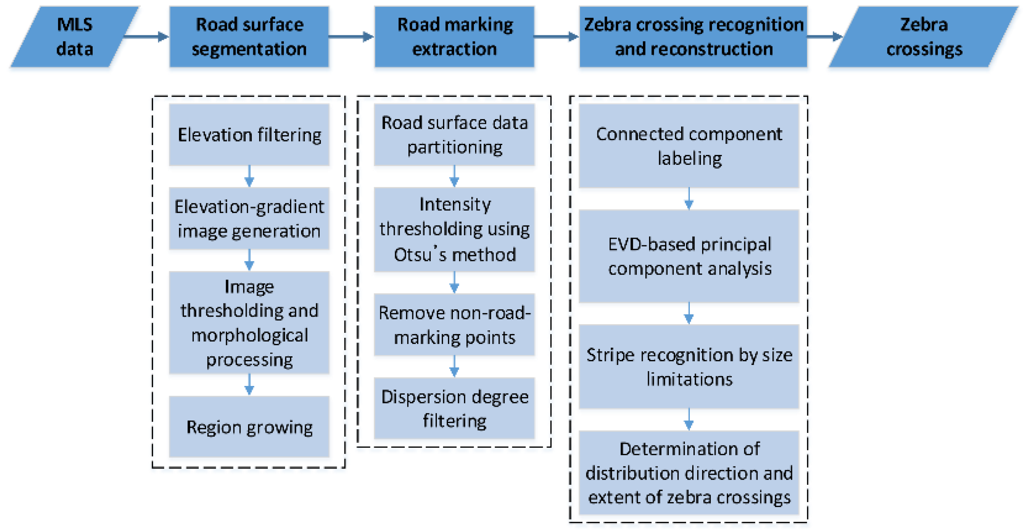
2. Method
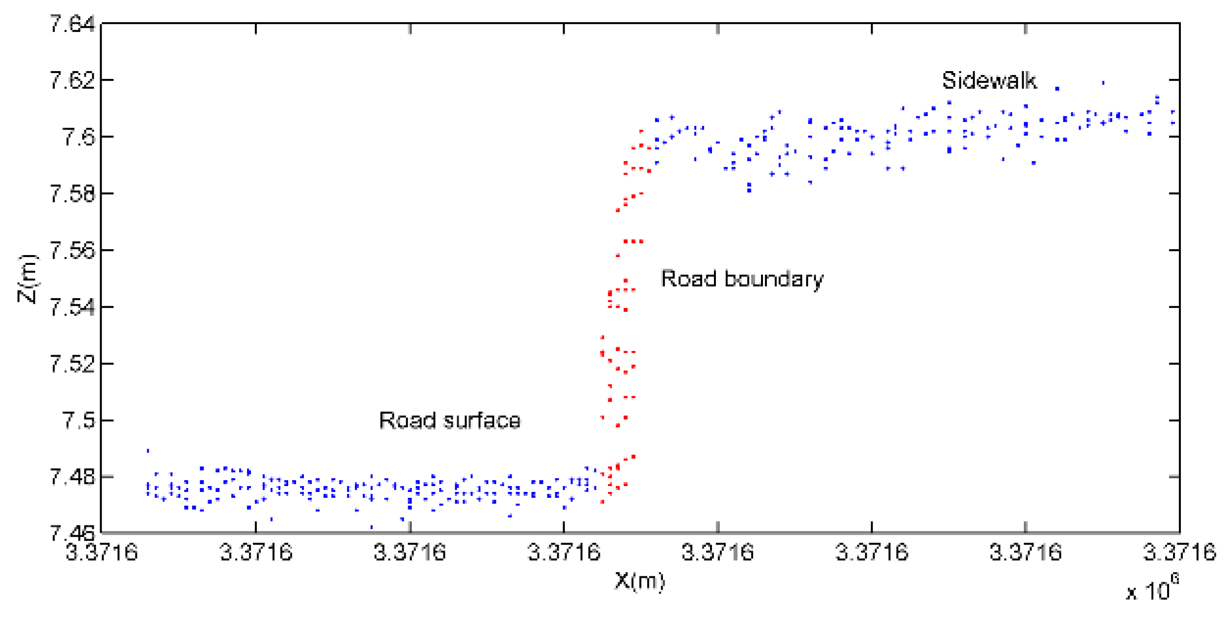
2.1. Road Surface Segmentation
2.1.1. Preprocessing
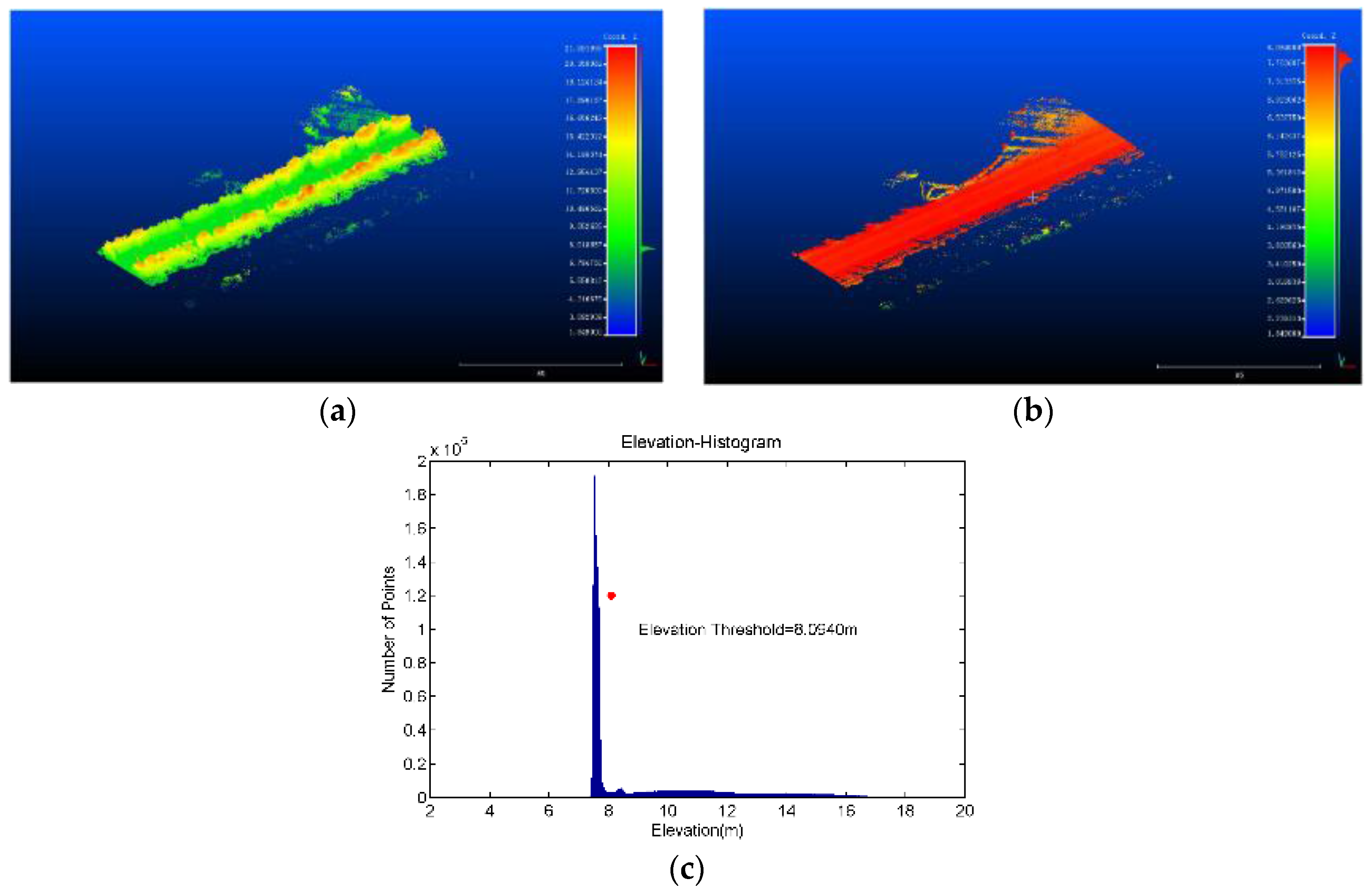
2.1.2. Elevation Filtering
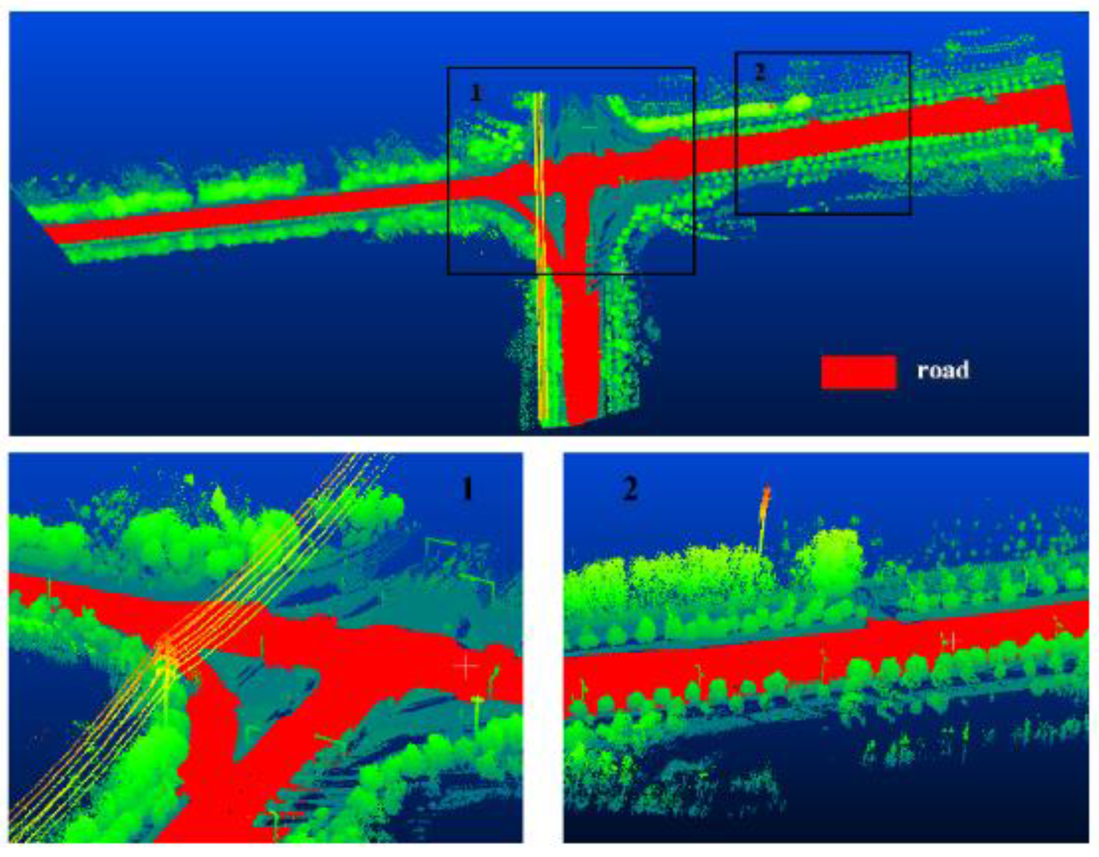
2.1.3. Segmentation by Region-Growing
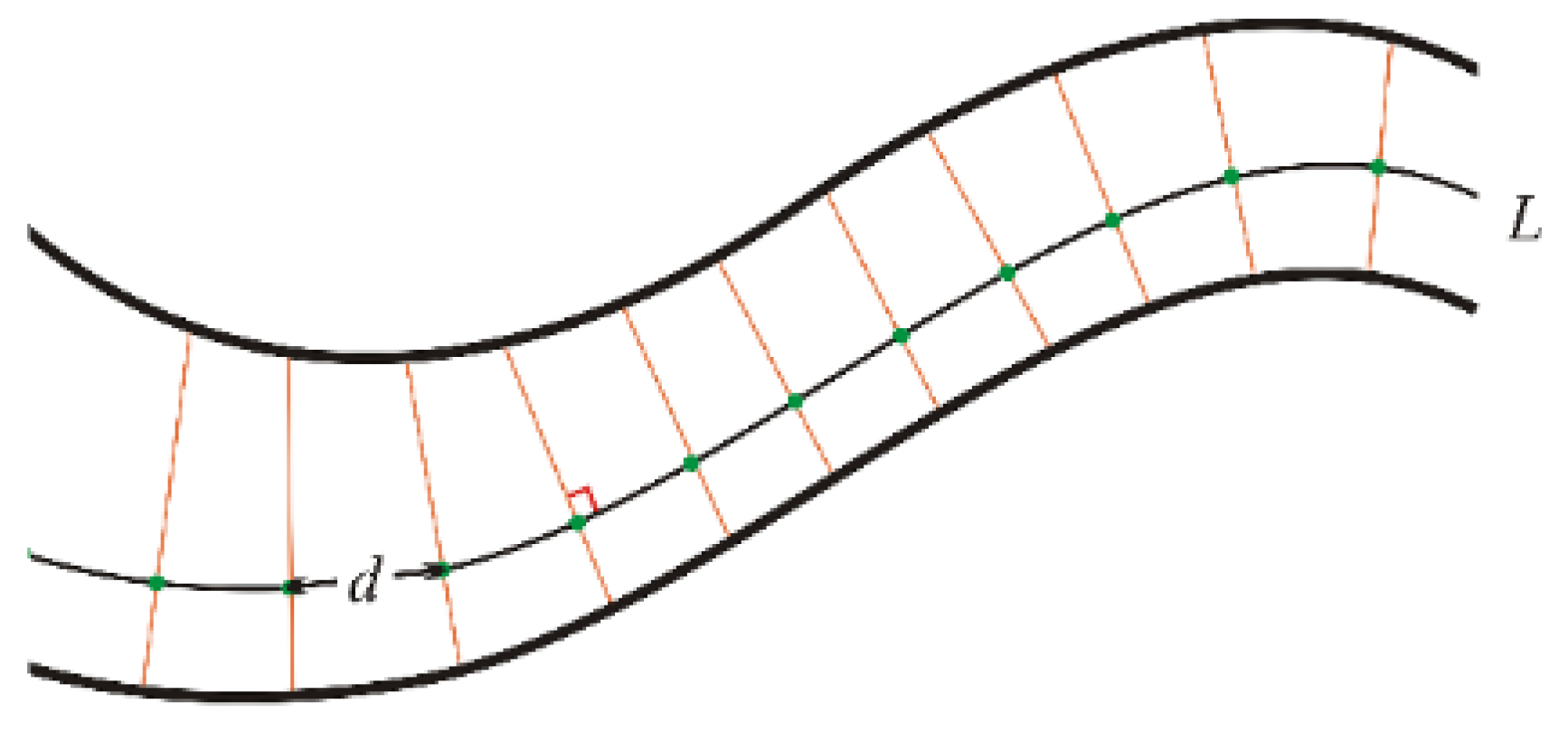
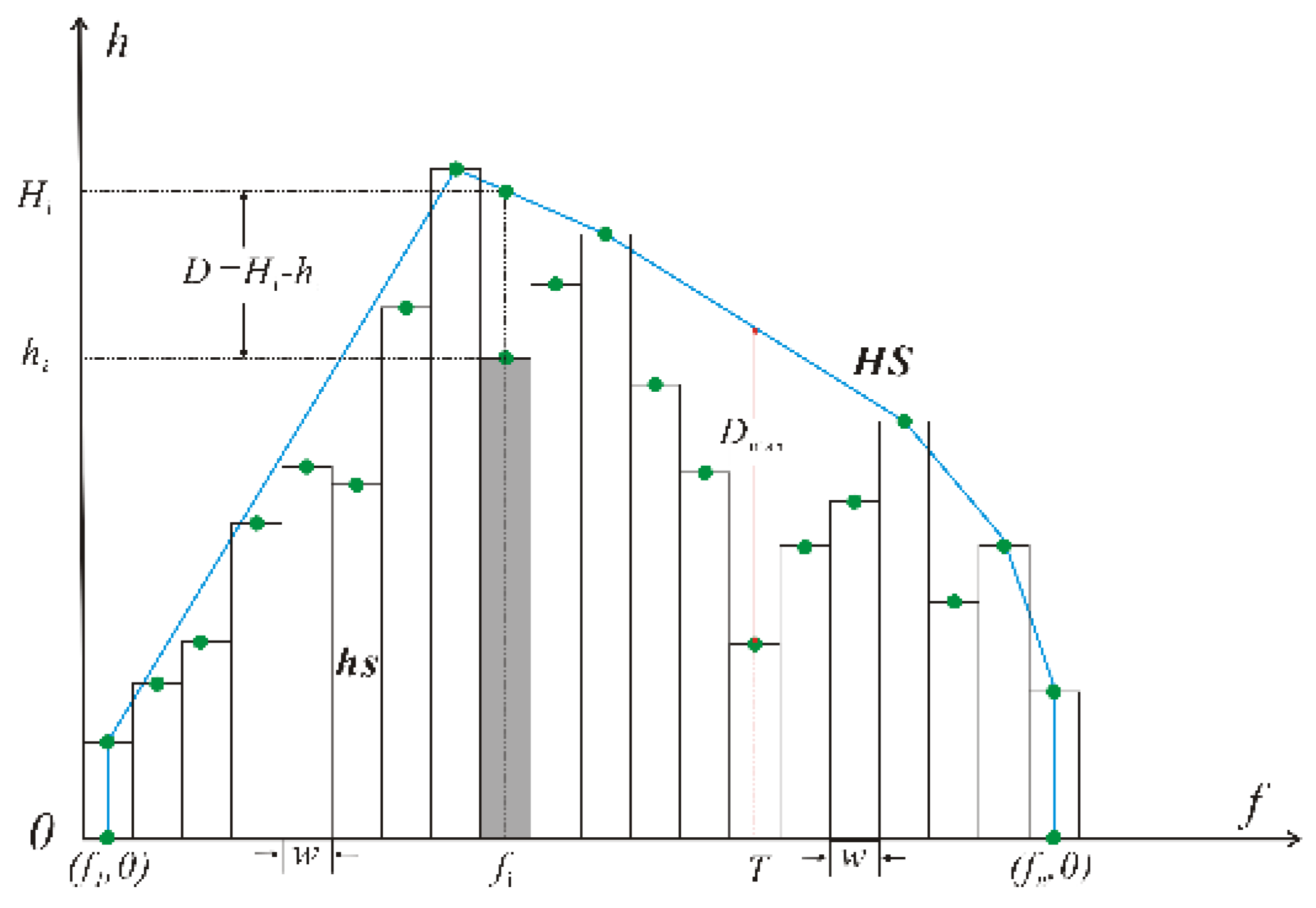
2.2. Road Marking Extraction
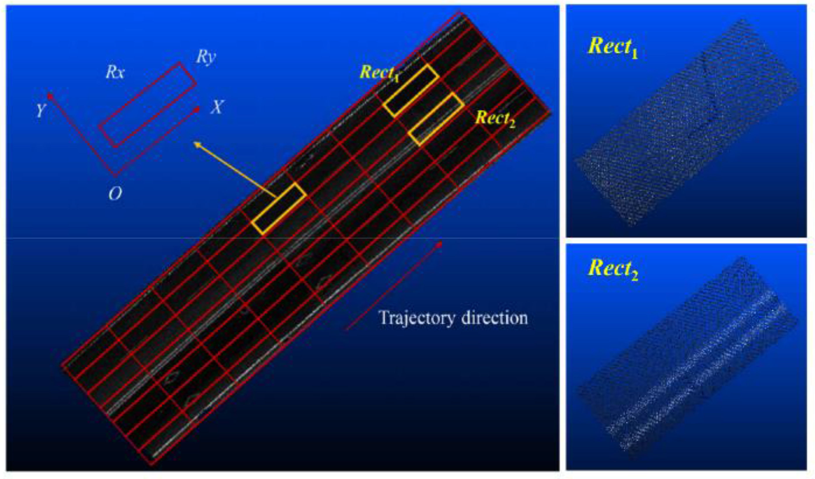
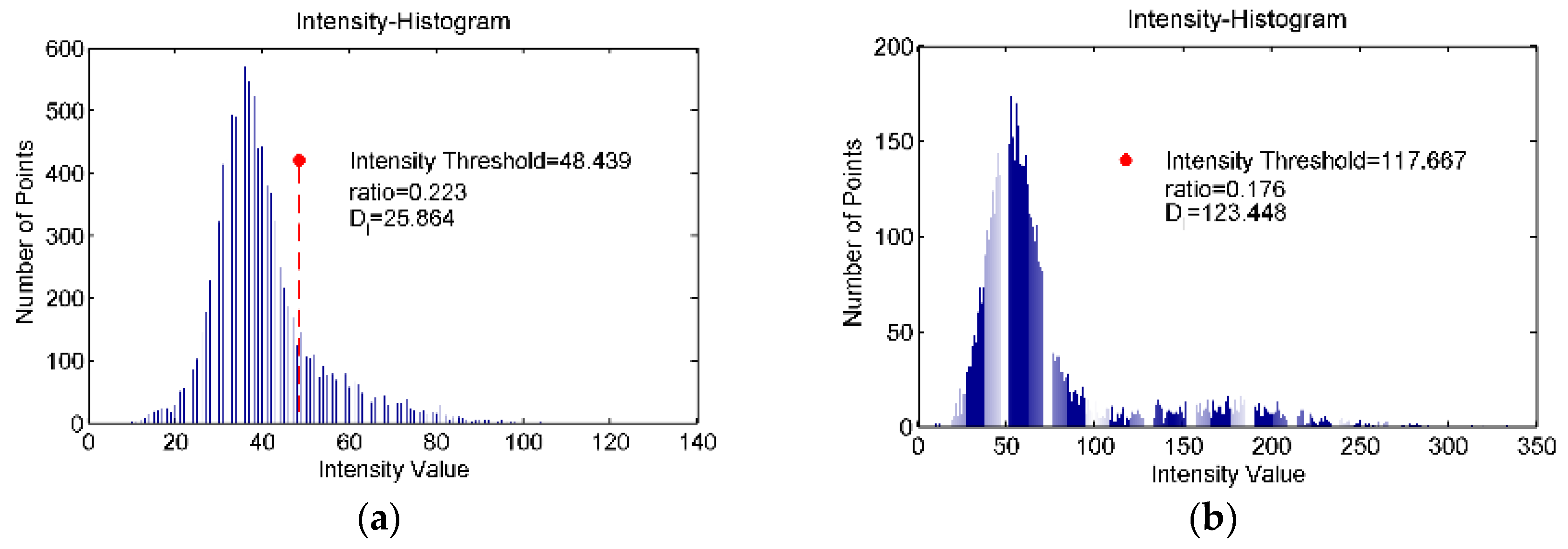
2.2.1. Adaptive Thresholding Based on Road Surface Partitioning
2.2.2. Dispersion Degree Filtering
2.3. Zebra Crossing Recognition and Construction
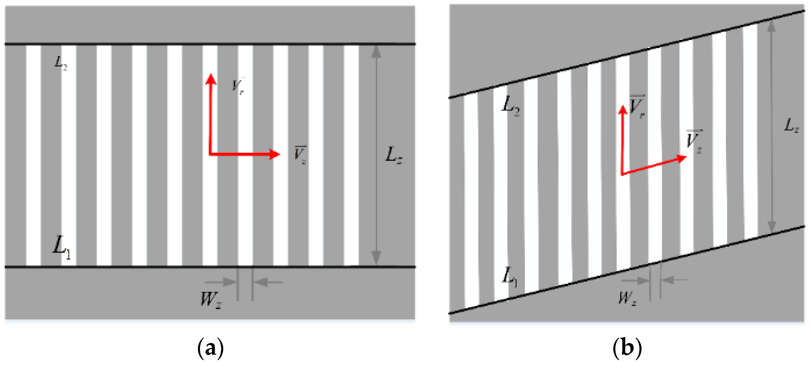
2.3.1. The Model of Zebra Crossings
2.3.2. Detection of Zebra Stripes
2.3.3. Reconstruction of Zebra Crossings
3. Results and Discussion
3.1. Segmentation of Road Surfaces
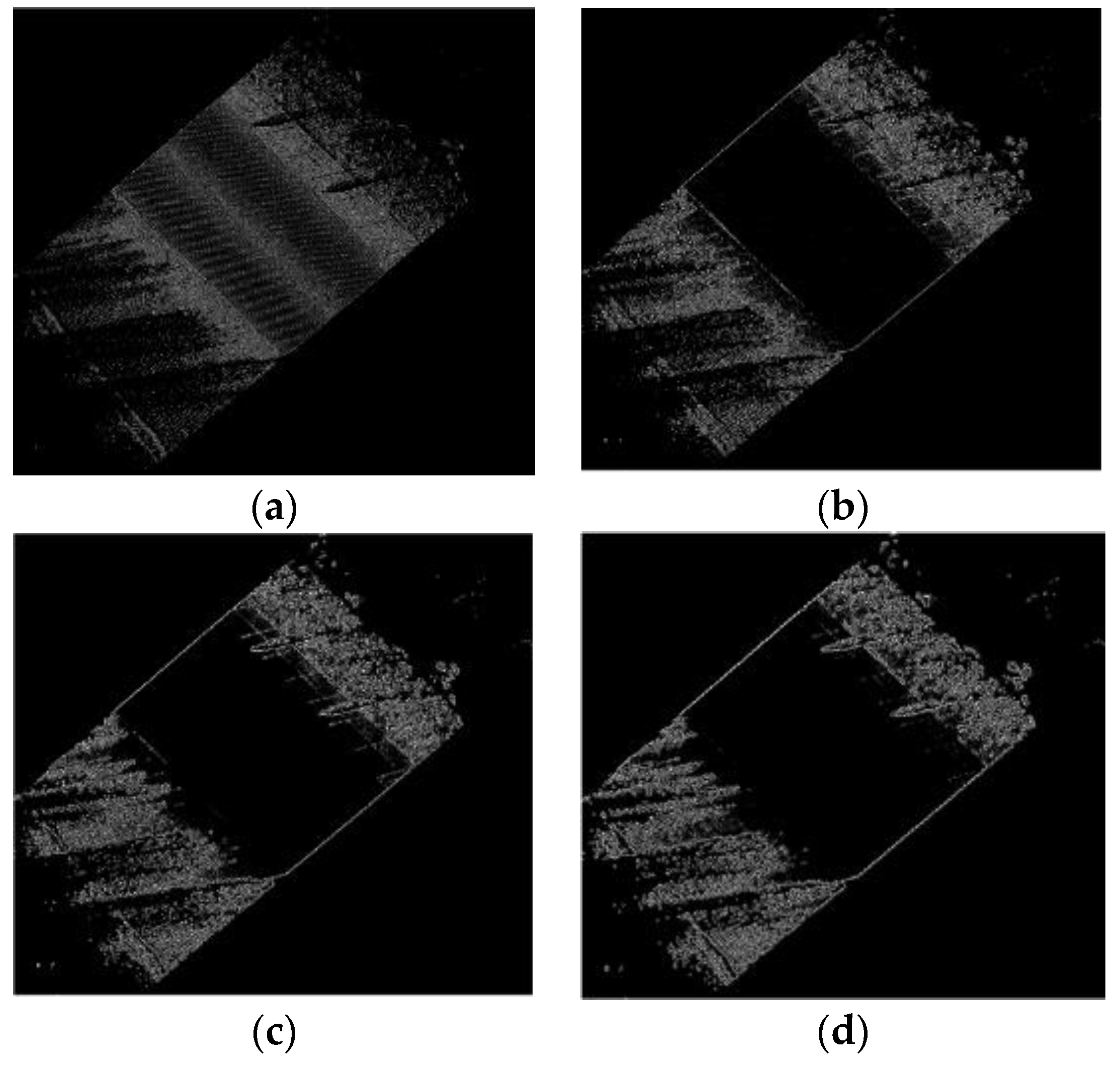
3.2. Extraction of Road Markings
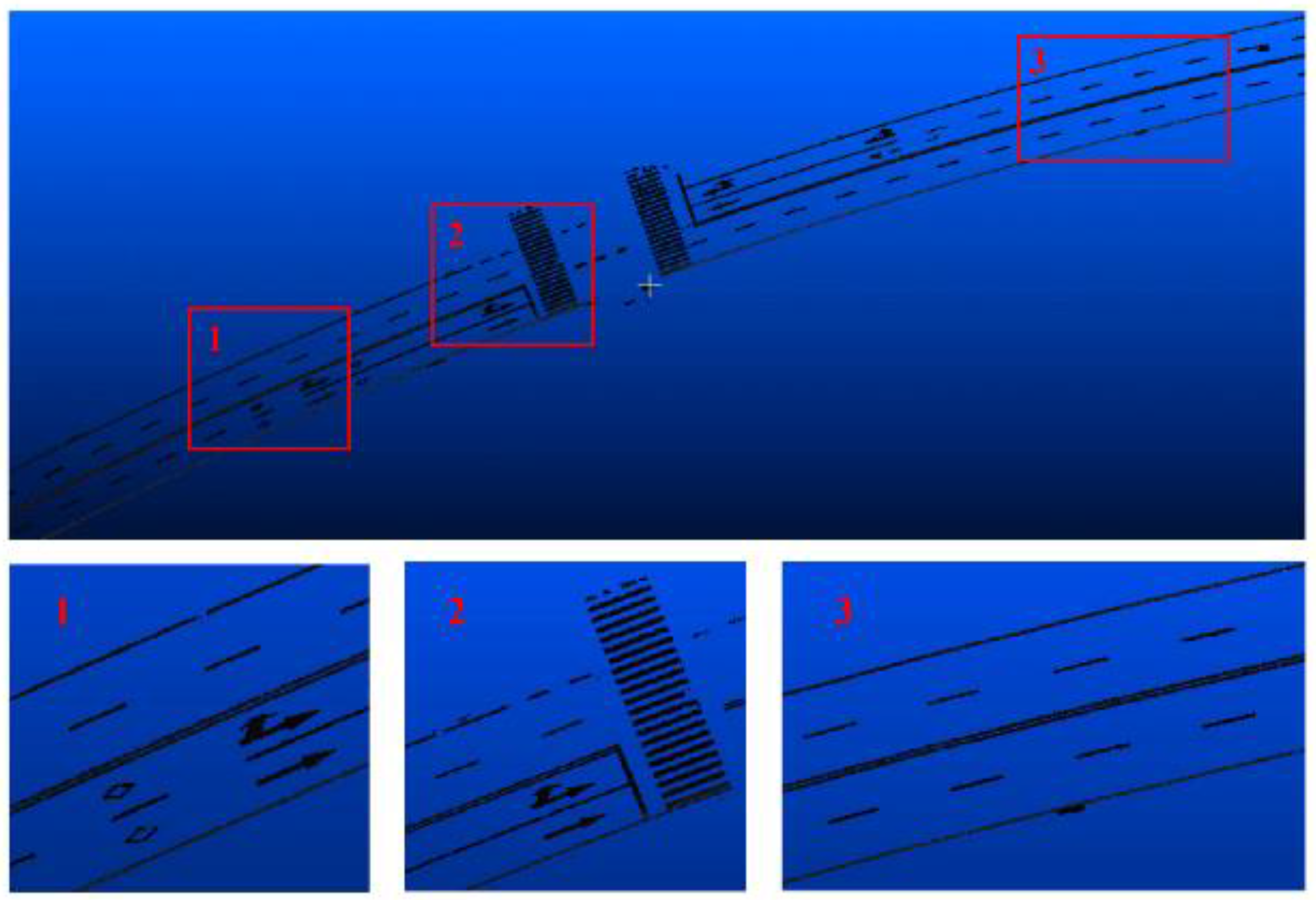
3.3. Recognition and Reconstruction of Zebra Crossings
4. Conclusions
Acknowledgments
Author Contributions
Conflicts of Interest
References
- China National Standardization Management Committee. GB 5768.3-2009: Road Traffic Signs and Markings. Part 3: Road Traffic Markings; China Standards Press: Beijing, China, 2009. [Google Scholar]
- Carnaby, B. Poor road markings contribute to crash rates. In Proceedings of Australasian Road Safety Research Policing Education Conference, Wellington, New Zealand, 14–16 November 2005.
- Horberry, T.; Anderson, J.; Regan, M.A. The possible safety benefits of enhanced road markings: A driving simulator evaluation. Transp. Res. Part F Traf. Psychol. Behav. 2006, 9, 77–87. [Google Scholar] [CrossRef]
- Zheng, N.-N.; Tang, S.; Cheng, H.; Li, Q.; Lai, G.; Wang, F.-Y. Toward intelligent driver-assistance and safety warning system. IEEE Intell. Syst. 2004, 19, 8–11. [Google Scholar] [CrossRef]
- McCall, J.C.; Trivedi, M.M. Video-based lane estimation and tracking for driver assistance: Survey, system, and evaluation. IEEE Trans. Intell. Transp. Syst. 2006, 7, 20–37. [Google Scholar] [CrossRef]
- Vacek, S.; Schimmel, C.; Dillmann, R. Road-marking analysis for autonomous vehicle guidance. In Proceedings of European Conference on Mobile Robots, Freiburg, Germany, 19–21 September 2007.
- Zhang, J.; Wang, F.-Y.; Wang, K.; Lin, W.-H.; Xu, X.; Chen, C. Data-driven intelligent transportation systems: A survey. IEEE Trans. Intell. Transp. Syst. 2011, 12, 1624–1639. [Google Scholar] [CrossRef]
- Bertozzi, M.; Bombini, L.; Broggi, A.; Zani, P.; Cerri, P.; Grisleri, P.; Medici, P. Gold: A framework for developing intelligent-vehicle vision applications. IEEE Intell. Syst. 2008, 23, 69–71. [Google Scholar] [CrossRef]
- Se, S.; Brady, M. Road feature detection and estimation. Mach. Vision Appl. 2003, 14, 157–165. [Google Scholar] [CrossRef]
- Chiu, K.-Y.; Lin, S.-F. Lane detection using color-based segmentation. In Proceedings of IEEE Conference on Intelligent Vehicles Symposium, Las Vegas, NV, USA, 6–8 June 2005; pp. 706–711.
- Sun, T.-Y.; Tsai, S.-J.; Chan, V. HSI color model based lane-marking detection. In Proceedings of Intelligent Transportation Systems Conference, Toronto, ON, Canada, 17–20 September 2006; pp. 1168–1172.
- Liu, W.; Zhang, H.; Duan, B.; Yuan, H.; Zhao, H. Vision-based real-time lane marking detection and tracking. In Proceedings of International IEEE Conferences on Intelligent Transportation Systems, Beijing, China, 12–15 October 2008; pp. 49–54.
- Soheilian, B.; Paparoditis, N.; Boldo, D. 3D road marking reconstruction from street-level calibrated stereo pairs. ISPRS J. Photogramm. 2010, 65, 347–359. [Google Scholar] [CrossRef]
- Foucher, P.; Sebsadji, Y.; Tarel, J.-P.; Charbonnier, P.; Nicolle, P. Detection and recognition of urban road markings using images. In Proceedings of International IEEE Conferences on Intelligent Transportation Systems, Washington, DC, USA, 5–7 October 2011; pp. 1747–1752.
- Wu, P.-C.; Chang, C.-Y.; Lin, C.H. Lane-mark extraction for automobiles under complex conditions. Pattern Recogn. 2014, 47, 2756–2767. [Google Scholar] [CrossRef]
- Fang, L.; Yang, B. Automated extracting structural roads from mobile laser scanning point clouds. Acta Geod. Cartogr. Sin. 2013, 2, 260–267. [Google Scholar]
- Zhao, H.; Shibasaki, R. Updating a digital geographic database using vehicle-borne laser scanners and line cameras. Photogramm. Eng. Remote Sens. 2005, 71, 415–424. [Google Scholar] [CrossRef]
- Vosselman, G. Advanced point cloud processing. In Proceedings of Photogrammetric week, Stuttgart, Germany, 7–11 September 2009; pp. 137–146.
- Yang, B.; Wei, Z.; Li, Q.; Mao, Q. A Classification-Oriented method of feature image generation for vehicle-borne laser scanning point clouds. Acta Geod. Cartogr. Sin. 2010, 39, 540–545. [Google Scholar]
- Wu, B.; Yu, B.; Huang, C.; Wu, Q.; Wu, J. Automated extraction of ground surface along urban roads from mobile laser scanning point clouds. Remote Sens. Lett. 2016, 7, 170–179. [Google Scholar] [CrossRef]
- Manandhar, D.; Shibasaki, R. Auto-extraction of urban features from vehicle-borne laser data. In Proceedings of Symposium on Geospatial Theory, Processing and Applications, Ottawa, ON, Canada; 2002; pp. 650–655. [Google Scholar]
- Li, B.; Li, Q.; Shi, W.; Wu, F. Feature extraction and modeling of urban building from vehicle-borne laser scanning data. Int. Arch. Photogramm. Remote Sens. Spat. Inf. Sci. 2004, 35, 934–939. [Google Scholar]
- Tournaire, O.; Brédif, M.; Boldo, D.; Durupt, M. An efficient stochastic approach for building footprint extraction from digital elevation models. ISPRS J. Photogramm. Remote Sens. 2010, 65, 317–327. [Google Scholar] [CrossRef]
- Lehtomäki, M.; Jaakkola, A.; Hyyppä, J.; Kukko, A.; Kaartinen, H. Detection of vertical pole-like objects in a road environment using vehicle-based laser scanning data. Remote Sens. 2010, 2, 641–664. [Google Scholar] [CrossRef]
- Wu, B.; Yu, B.; Yue, W.; Shu, S.; Tan, W.; Hu, C.; Huang, Y.; Wu, J.; Liu, H. A voxel-based method for automated identification and morphological parameters estimation of individual street trees from mobile laser scanning data. Remote Sens. 2013, 5, 584–611. [Google Scholar] [CrossRef]
- Li, L.; Li, Y.; Li, D. A method based on an adaptive radius cylinder model for detecting pole-like objects in mobile laser scanning data. Remote Sens. Lett. 2016, 7, 249–258. [Google Scholar] [CrossRef]
- Jaakkola, A.; Hyyppä, J.; Hyyppä, H.; Kukko, A. Retrieval algorithms for road surface modelling using laser-based mobile mapping. Sensors 2008, 8, 5238–5249. [Google Scholar] [CrossRef]
- Yang, B.; Fang, L.; Li, Q.; Li, J. Automated extraction of road markings from mobile LiDAR point clouds. Photogramm. Eng. Remotr Sens. 2012, 78, 331–338. [Google Scholar] [CrossRef]
- Kammel, S.; Pitzer, B. Lidar-based lane marker detection and mapping. In Proceedings of IEEE on Intelligent Vehicles Symposium, Eindhoven, The Netherlands, 4–6 June 2008; pp. 1137–1142.
- Chen, X.; Kohlmeyer, B.; Stroila, M.; Alwar, N.; Wang, R.; Bach, J. Next generation map making: Geo-referenced ground-level LiDAR point clouds for automatic retro-reflective road feature extraction. In Proceedings of the 17th ACM SIGSPATIAL International Conference on Advances in Geographic Information Systems, Seattle, WA, USA, 4–6 November 2009; pp. 488–491.
- Smadja, L.; Ninot, J.; Gavrilovic, T. Road extraction and environment interpretation from LiDAR sensors. In Proceedings of International Archives of the Photogrammetry, Remote sensing and Spatial Information Sciences, Saint-Mande, France, 1–3 September 2010; pp. 281–286.
- Guan, H.Y.; Li, J.; Yu, Y.T.; Wang, C.; Chapman, M.; Yang, B.S. Using mobile laser scanning data for automated extraction of road markings. ISPRS J. Photogramm. Remote Sens. 2014, 87, 93–107. [Google Scholar] [CrossRef]
- Mancini, A.; Frontoni, E.; Zingaretti, P. Automatic road object extraction from mobile mapping systems. In Proceedings of IEEE/ASME International Conference on Mechatronics and Embedded Systems and Applications (MESA), Suzhou, Jiangsu, China, 8–10 July 2012; pp. 281–286.
- Riveiro, B.; González-Jorge, H.; Martínez-Sánchez, J.; Díaz-Vilariño, L.; Arias, P. Automatic detection of zebra crossings from mobile LiDAR data. Opt. Laser Technol. 2015, 70, 63–70. [Google Scholar] [CrossRef]
- Yu, Y.; Li, J.; Guan, H.; Jia, F.; Wang, C. Learning hierarchical features for automated extraction of road markings from 3-d mobile LiDAR point clouds. IEEE J. Sel. Top. Appl. 2015, 8, 709–726. [Google Scholar] [CrossRef]
- Rosenfeld, A.; De La Torre, P. Histogram concavity analysis as an aid in threshold selection. IEEE Trans. Syst. Man Cybern. 1983, SMC-13, 231–235. [Google Scholar] [CrossRef]
- Franke, R.; Nielson, G. Smooth interpolation of large sets of scattered data. Int. J. Numer. Meth. Eng. 1980, 15, 1691–1704. [Google Scholar] [CrossRef]
- Otsu, N. A threshold selection method from gray-level histograms. Automatica 1975, 11, 23–27. [Google Scholar]
- Fischler, M.A.; Bolles, R.C. Random sample consensus: A paradigm for model fitting with applications to image analysis and automated cartography. Commun. ACM 1981, 24, 381–395. [Google Scholar] [CrossRef]


| Dataset | Length/(m) | Number of Points |
|---|---|---|
| 1 | 1200 | 45,175,744 |
| 2 | 1350 | 43,407,389 |
| 3 | 600 | 16,624,370 |
| Name | Value | Name | Value |
|---|---|---|---|
| Rx | 2 m | Tr | 0.8 |
| Ry | 1 m | NP | 5 |
| Td | 40 | TD | 0.007 m |
| Dataset | Number of Zebra Crossings | Recognition Rate of the Proposed Method (%) | Recognition Rate of Riveiro’s Method (%) |
|---|---|---|---|
| 1 | 3 | 100.00 | 66.67 |
| 2 | 6 | 100.00 | 66.67 |
| 3 | 2 | 50.00 | 50.00 |
| Total | 11 | 90.91 | 63.64 |
| Dataset | Zebra crossing | r (%) | p (%) | θz (°) | θr (°) |
|---|---|---|---|---|---|
| 1 | 1 | 95.97 | 96.25 | 2.50 | 1.20 |
| 1 | 2 | 96.60 | 99.57 | 0.87 | 0.24 |
| 1 | 3 | 99.08 | 95.45 | 0.08 | 0.06 |
| 2 | 1 | 94.55 | 94.20 | 1.00 | 0.02 |
| 2 | 2 | 91.70 | 97.87 | 0.28 | 0.15 |
| 2 | 3 | 92.68 | 98.67 | 0.33 | 0.03 |
| 2 | 4 | 95.69 | 91.94 | 0.50 | 0.44 |
| 2 | 5 | 96.56 | 98.84 | 1.51 | 0.17 |
| 2 | 6 | 96.40 | 98.93 | 1.51 | 0.46 |
| 3 | 1 | 97.03 | 94.54 | 0.74 | 0.05 |
| 3 | 2 | / | / | / | / |
© 2016 by the authors; licensee MDPI, Basel, Switzerland. This article is an open access article distributed under the terms and conditions of the Creative Commons Attribution (CC-BY) license (http://creativecommons.org/licenses/by/4.0/).
Share and Cite
Li, L.; Zhang, D.; Ying, S.; Li, Y. Recognition and Reconstruction of Zebra Crossings on Roads from Mobile Laser Scanning Data. ISPRS Int. J. Geo-Inf. 2016, 5, 125. https://0-doi-org.brum.beds.ac.uk/10.3390/ijgi5070125
Li L, Zhang D, Ying S, Li Y. Recognition and Reconstruction of Zebra Crossings on Roads from Mobile Laser Scanning Data. ISPRS International Journal of Geo-Information. 2016; 5(7):125. https://0-doi-org.brum.beds.ac.uk/10.3390/ijgi5070125
Chicago/Turabian StyleLi, Lin, Da Zhang, Shen Ying, and You Li. 2016. "Recognition and Reconstruction of Zebra Crossings on Roads from Mobile Laser Scanning Data" ISPRS International Journal of Geo-Information 5, no. 7: 125. https://0-doi-org.brum.beds.ac.uk/10.3390/ijgi5070125