Analyzing Local Spatio-Temporal Patterns of Police Calls-for-Service Using Bayesian Integrated Nested Laplace Approximation

Abstract

This research investigates spatio-temporal patterns of police calls-for-service in the Region of Waterloo, Canada, at a fine spatial and temporal resolution. Modeling was implemented via Bayesian Integrated Nested Laplace Approximation (INLA). Temporal patterns for two-hour time periods, spatial patterns at the small-area scale, and space-time interaction (i.e., unusual departures from overall spatial and temporal patterns) were estimated. Temporally, calls-for-service were found to be lowest in the early morning (02:00–03:59) and highest in the evening (20:00–21:59), while high levels of calls-for-service were spatially located in central business areas and in areas characterized by major roadways, universities, and shopping centres. Space-time interaction was observed to be geographically dispersed during daytime hours but concentrated in central business areas during evening hours. Interpreted through the routine activity theory, results are discussed with respect to law enforcement resource demand and allocation, and the advantages of modeling spatio-temporal datasets with Bayesian INLA methods are highlighted.

1. Introduction

In law enforcement, the implementation of computer-aided dispatch systems that automatically record location- and time-specific information for police calls-for-service has facilitated the storage, retrieval, and analysis of large volumes of spatio-temporal data [1,2,3,4,5]. Paired with technological advances in geographic information systems, crime mapping, or the analysis and visualization of historical spatial and temporal police call-for-service patterns, has become an important part of police operations and strategy [6]. Police calls-for-service encompass reported crimes, emergency response, traffic management, and other police-facilitated services [6], and compared to official crime data, provide a more comprehensive indicator of overall police resource demand. Increasingly, call-for-service data is available at fine spatial and temporal resolutions, enabling detailed analysis of local Space-time variation.

Past crime mapping research at the small-area scale often analyzes spatial and temporal patterns separately. Purely spatial analyses identify hotspots, or groups of small areas that exhibit clustering or high-spatial autocorrelation [7]. Assuming a null hypothesis of spatial randomness (i.e., no spatial autocorrelation) a variety of statistical tests have been applied to identify spatial clusters of crime or calls-for-service, including the Getis-Ord statistic [8], local Moran’s I [9,10], the spatial scan statistic [11,12], and the spatial point pattern test [13]. Purely temporal analyses, on the other hand, fit time trends to small-area data. One popular method is the group-based trajectory analysis, which uses mathematical functions (i.e., linear, quadratic) to generalize long-term time trends [14,15], but treats small-area data as independent and does not account for local spatial autocorrelation.

Purely spatial and purely temporal methods do not simultaneously analyze variation in space and time and, consequently, do not identify space-time interaction. Space-time interaction is defined as residual space-time clustering after accounting for overall spatial and temporal patterns, and is estimated for each space-time unit of analysis [16,17,18]. In this research context, areas with high space-time interaction for a given time period may be highlighted as areas that exhibit unusually high levels of calls-for-service above baseline spatial and temporal risk. Space-time interaction helps to uncover patterns that may be overlooked in purely spatial or temporal analyses and that may be associated with, for example, long-term changes in local socioeconomic conditions or social disorganization [19], changes to drug market conditions or resident perceptions of law enforcement [20,21], or short-term changes in policing strategy [22].

Broadly, methods of spatio-temporal analysis can be classified as testing- or model-based [16]. Testing-based approaches provide one test statistic for the study region that quantifies relative clustering in both space and time [23]. For point data, two popular approaches are the Knox and Jacquez tests, which count the number of point pairs that occur within specified spatial and temporal thresholds, with the former based on user-chosen thresholds and the latter based on nearest-neighbour thresholds [17,18,24]. For small-area data, the space-time scan statistic first identifies spatial hotspots based on the difference between observed and expected counts within ellipses centred at small-area centroids, and extends the spatial ellipse over time to analyze the persistence of spatial hotpots [11,25]. While useful for identifying overall levels of space-time clustering for a dataset, testing-based methods do not identify overall spatial and temporal patterns (i.e., for the study region) and do not provide risk estimates for observations not identified as hotspots.

Model-based spatio-temporal methods for small-area data decompose observed space-time data into overall spatial and overall temporal patterns, as well as space-time interaction. Estimates of these components are not feasible by comparing maps or count or rate data, particularly when the number of space-time units is large. Conceptually, space-time models resemble regression models, where the outcome variable (i.e., count of calls-for-service) is estimated through a number of parameters including spatial, temporal, and spatio-temporal random effects [26]. Models with many random effects parameters are often implemented in a Bayesian framework [27]. Briefly, Bayesian methods combine observed data (i.e., space-time incident counts) and prior information (i.e., spatial and temporal structures) to estimate posterior probability distributions of model parameters, including space-time interaction [28].

Random effects parameters can be interpreted as surrogates for unmeasured spatial, temporal, or space-time processes. Spatial random effects, for example, represent spatially autocorrelated covariates and are often specified via conditional autoregressive (CAR) processes [29]. CAR processes assume that the mean of the spatial random effects parameter in a given area is conditional on spatial random effects estimates in geographically adjacent areas. This is often referred to as “borrowing strength” [30]. The CAR model has been used extensively in ecological studies to analyze health-related outcomes [31,32,33] as well as crime [34,35,36]. The CAR process can be conveniently applied to temporal data, where temporal random effects for a time period is conditional on the mean values of temporal random effects at time periods both before and after [37,38].

Applying Bayesian models to analyze spatio-temporal datasets is computationally challenging using conventional Markov chain Monte Carlo (MCMC) algorithms [39,40] because MCMC requires iterative assessment of various full conditional density functions and monitoring convergence of posterior probability distributions requires extensive simulation [41,42]. Recently, the Integrated Nested Laplace Approximation (INLA) method has been proposed, which approximates posterior probability distributions via numerical integration rather than an MCMC-based iterative process [28,43]. Past research comparing MCMC and INLA approaches has found that INLA reduces computational time and retains reliable parameter estimates [28]. Computational efficiency is important when analyzing spatio-temporal data because various prior distributions and assumptions for spatial, temporal, and Space-time random effects parameters can be tested and compared [44].

This research analyzes spatio-temporal patterns of police calls-for-service at the small-area level in the Region of Waterloo, Canada. Calls-for-service for one year (2011) were temporally aggregated to 12 time periods of 2 hours, representing a 24 hour day, and geographically aggregated to 755 census dissemination areas, resulting in a total of 9060 Space-time units. Aggregated calls-for-service were analyzed to provide broad insight into the Space-time patterns of law enforcement resources and because this provides sufficient count data to capture meaningful spatial, temporal, and Space-time patterns at this resolution. Hourly patterns were analyzed because crime and police resources have been shown to vary by hour of day more than any other predictor [45] and anticipated spatial and temporal autocorrelation can be appropriately accounted for via CAR processes.

This paper first reviews the study region and call-for-service data. Next, the spatio-temporal model is detailed and four types of space-time interactions are described, each of which holds specific assumptions regarding the spatial and/or temporal structure of residual space-time patterns. Overall spatial and overall temporal patterns, as well as space-time interaction and space-time hotspots, are visualized, interpreted through the routine activity theory, and discussed in the contexts of understanding and informing police resource allocation. In conclusion, we reflect on the use of Bayesian spatio-temporal models and INLA to model spatio-temporal datasets.

2. Study Region

The Regional Municipality of Waterloo, Ontario, Canada, is composed of the cities of Waterloo, Kitchener, and Cambridge, as well as four rural townships. In 2011, the region had a population of 506,107 distributed across 755 census dissemination areas (DAs). For reference, DAs are the smallest areal units that cover the entirety of Canada and are delineated such that residential populations are between 400 and 700 [46].

3. Police Call-for-Service Data

Call-for-service data were provided by the Waterloo Regional Police Service for 1 January 2011 to 31 December 2011. Calls-for-service include violent crimes (count = 2696), property crimes (13,704), disorder (18,949), bylaw complaints (10,598), motor-vehicle-related calls (31,105), 911 calls (65,617), and a variety of other police-related services [47,48]. Locations reflect the closest intersection to call location and calls were summed to the DA-scale. Descriptive statistics for total calls-for-service are shown in

Table 1. Descriptive statistics for call-for-service counts in Waterloo Region, 2011.

	Study Region	Dissemination Area
	Total Count	Mean	Min.	Max.	Std. Dev.
Population	507,096	671.65	5	4698	462.78
Total calls-for-service	290,275	384.47	0	42,912	1623.68
Expected calls-for-service	290,275 1	384.47	2.86	2689.26	264.91

¹ Expected total count and mean values are equal to observed count and mean values.

. Expected counts were calculated as the product of study region rate and DA population (= (total call-for-service count/total population) x DA population) to reflect underlying population variation.

In general, areas with high total counts were located in the centre of the study region, closely corresponding to the central business areas of Waterloo, Kitchener, and Cambridge, as well as in areas towards the periphery of the study region in the east and south (Figure 1A). Compared to observed counts, expected counts were lower in central business areas but higher in areas adjacent to central business areas (i.e., areas that have larger residential populations) (Figure 1B).

Temporally, calls-for-service were categorized into 12 time periods, each representing 2 hours of a 24 hour day (

Table 2. Descriptive statistics for the temporal variation of calls-for-service. Note that 00:00 refers to midnight and 12:00 refers to noon.

Time Period	Mean	Min.	Max.	Std. Dev.
00:00 to 01:59	29.81	0	1987	88.04
02:00 to 03:59	19.31	0	1229	57.86
04:00 to 05:59	10.80	0	850	36.14
06:00 to 07:59	18.22	0	2015	76.87
08:00 to 09:59	39.02	0	3951	155.97
10:00 to 11:59	40.96	0	4310	164.22
12:00 to 13:39	38.87	0	5035	190.14
14:00 to 15:59	44.77	0	5718	214.58
16:00 to 17:59	40.95	0	5718	215.58
18:00 to 19:59	36.01	0	5100	188.78
20:00 to 21:59	33.78	0	4195	156.10
22:00 to 23:59	31.98	0	2985	116.13

). Calls were highest during afternoon and evening hours and lowest in the early morning (Figure 2). In total, there were 290,027 calls-for-service distributed over 9060 space-time units (= 755 DAs × 12 time periods).

The spatial patterns of calls-for-service are shown in Figure 3 for 04:00–05:59 (Figure 3A), the time period with the lowest observed count, and for 14:00–15:59 (Figure 3B), the time period with the highest observed count. Compared to 14:00–15:59, there were fewer areas with high counts (>50) during 04:00–05:59 and high-count areas were located closer to the main transportation corridor connecting Waterloo, Kitchener, and Cambridge. From 14:00 to 15:59, there were many more areas with high call-for-service counts and these areas were geographically dispersed throughout the study region.

4. Spatio-Temporal Modeling

Bayesian spatial and spatio-temporal models are often hierarchical with three levels [39]. In this context, hierarchical is used to describe the structure of Bayesian models: the first level models the observed data with a likelihood function (probability distribution) and specifies a process model that includes spatial, temporal, and space-time random effects; the second level assigns prior distributions for model parameters; and the third level specifies hyperpriors for parameters of second-level prior distributions (e.g., variances). Prior distributions quantify researcher uncertainty in parameter estimates and impose spatial and/or temporal structure for random effects parameters [30,49].

At the first level, call-for-service count for small-area i (1, …, 755) and time period t (1, …, 12) is represented by O_it and sampled from a Poisson distribution (Equation (1)). The Poisson mean, μ_it, is the product of expected call-for-service count (E_it) and relative risk (r_it) (Equation (2)). Poisson models are common in spatial and spatio-temporal analysis of count data at the small-area scale [50].

O_it~Poisson(μ_it)

(1)

μ_it = E_it × r_it

(2)

Equation (3) decomposes relative risk into overall risk for the study region (α) and spatial, temporal, and space-time random effects. This is the general nonparametric model structure used for space-time analysis [44]. The parametric structure models space-time interaction by incorporating a time covariate that assumes linearity [44,51]. Main spatial effects (u_i + s_i) measure the spatial pattern of calls-for-service and account for spatial autocorrelation and overdispersion [52]. Main temporal effects (γ_t + φ_t) capture overall time trend for the study region. Space-time interaction (Ψ_it) measures departures from main spatial and main temporal effects.

log(μ_it) = log(E_it) + α + u_i + s_i + γ_t + φ_t + Ψ_it

(3)

4.1. Prior Distributions

A vague prior of a normal distribution with mean 0 and variance 1000 was specified for α. Vague priors provide little information and let the observed data dominate posterior estimates. The prior for unstructured spatial effects (u_i) was a normal distribution with mean zero and variance ${\sigma }_{\mathrm{u}}^2$ (Equation (4a)). Spatially structured random effects (s_i) detect spatial autocorrelation and were assigned an intrinsic conditional autoregressive (ICAR) prior distribution, with spatial adjacency matrix W and variance ${\sigma }_{\mathrm{s}}^2$ (Equation (4b)). For reference, W is a symmetrical matrix where adjacency for a given small area includes all small areas sharing a vertex. ICAR is a common prior distribution for spatial random effects parameters, where the expected mean of s_i is equal to the mean of adjacent s_i’s [29,52,53]. The variance of s_i is controlled by ${\sigma }_{\mathrm{s}}^2$ and is inversely proportional to the number of neighbors of area i. Note that the ICAR prior imposes spatial structure.

$${\mathrm{u}}_{\mathrm{i}}~\mathrm{Normal}(0, {\mathsf{\sigma }}_{\mathrm{u}}^2)$$

(4a)

$${\mathrm{s}}_{\mathrm{i}}~\mathrm{ICAR}(\mathrm{W}, {\mathsf{\sigma }}_{\mathrm{s}}^2)$$

(4b)

Unstructured temporal effects (γ_t) were assigned a prior of a normal distribution with mean zero and variance ${\sigma }_{\mathsf{\gamma }}^2$ (Equation (5a)). Similar to s_i, the prior distribution for structured temporal effects (φ_t) was an ICAR process with temporal weight matrix P and variance ${\sigma }_{\mathsf{\varphi }}^2$, where φ_t borrows strength from adjacent time periods (Equation (5b)). This is analogous to the spatial ICAR model (Equation (4a,b)). Alternative priors where temporal adjacency is conditional only on previous time periods are available [54,55], however ICAR was considered suitable in this context because calls-for-service at time t should be correlated with incidents at both t − 1 and t + 1 [18].

$${\mathsf{\gamma }}_{\mathrm{t}}~\mathrm{Normal}(0, {\mathsf{\sigma }}_{\mathsf{\gamma }}^2)$$

(5a)

$${\mathsf{\varphi }}_{\mathrm{t}}~\mathrm{ICAR}(\mathrm{P}, {\mathsf{\sigma }}_{\mathsf{\varphi }}^2)$$

(5b)

Without prior information regarding residual space-time structure, we tested four prior distributions for Ψ_it. Each imposes different assumptions regarding spatial and/or temporal structure [44]. Testing many types of space-time interaction would generally be prohibitively time consuming using MCMC-based algorithms, however INLA enables efficient analysis and model checking of multiple prior distributions.

Type I space-time interaction assumes that Ψ_it for each space-time unit is exchangeable and independently and identically distributed (i.e., u_i and γ_t interact, as shown in Equation (3)). This type of space-time interaction is suitable in the case that residual space-time patterns in calls-for-service for a given space-time unit of analysis are not correlated with adjacent areas or times. Type II interaction is composed of spatially unstructured but temporally structured effects, assuming that small-area incident risk is similar over time but independent in space such that adjacent areas do not have similar patterns of calls-for-service (i.e., u_i and φ_t interact). Type III interaction is composed of spatially structured but temporally unstructured effects and assumes that small-area incident risk exhibits spatial autocorrelation for each time period but are independent in time (i.e., s_i and γ_t interact). Type IV space-time interaction captures both spatial and temporal structure and assumes that calls-for-service for a space-time unit of analysis are both spatially and temporally correlated (i.e., s_i and φ_t interact) [40,44]. This specification is reasonable when the trend of calls-for-service for one area is similar over time and geographically adjacent areas exhibit similar trends. The variance for all types of Ψ_it is controlled by ${\sigma }_{\mathsf{\Psi }}^2$. Further details regarding the assumptions and modeling of inseparable space-time interaction can be found in Knorr-Held [44].

4.2. Hyperprior Distributions

The third level of this Bayesian hierarchical model specifies prior distributions for variance parameters of second-level prior distributions. These are referred to as hyperprior distributions. All precision parameters (the reciprocal of variance) were assigned a vague Gamma(0.5, 0.0005) distribution [56]. All models were tested with hyperprior distributions of Gamma(0.001, 0.001) to ensure that results were not sensitive to hyperprior specification.

4.3. Model Implementation and Goodness-of-Fit

Modeling was completed in R using the R-INLA package [43] and results were exported and mapped in Quantum GIS 2.14. The Deviance Information Criterion (DIC) was used to assess model fit [57]. Broadly, DIC is a Bayesian analogue of the Akaike Information Criterion and balances model goodness-of-fit and complexity [58]. Smaller DIC values by at least five units indicate superior model fit [57]. DIC is shown in Equation (6), where $\overline{\mathrm{D}}$ is the mean deviance and ${\mathrm{p}}_{\mathrm{D}}$ is effective number of parameters, or the mean deviance ($\overline{\mathrm{D}}$) minus the deviance evaluated at the posterior estimated values ($\widehat{\mathrm{D}}$) (Equation (7)). Of note, highly correlated parameters (i.e., space, time or Space-time random effects) are often counted as less than one “effective parameter” in DIC calculations [59].

$$\mathrm{DIC}=\overline{\mathrm{D}}+{\mathrm{p}}_{\mathrm{D}}$$

(6)

$${\mathrm{p}}_{\mathrm{D}}=\overline{\mathrm{D}}-\widehat{\mathrm{D}}$$

(7)

5. Results

DIC values and the number of effective parameters (p_D) for the four spatio-temporal models testing space-time interaction are shown in

Table 3. Deviance Information Criterion (DIC) values for models with Type I, II, III, and IV space-time interaction.

Space-Time Interaction	Interaction Parameters	DIC	pD
Type I	ui and γt	54,099	5,010
Type II	ui and φt	53,630	4556
Type III	si and γt	53,997	4678
Type IV	si and φt	53,470	4311

. Note that DIC values from the models testing Type I, II, III, and IV space-time interaction do not exhibit extreme differences. This can be attributed to all models taking the form shown in Equation (3), but differing with respect to the prior distributions of the space-time interaction parameters.

The model analyzing Type IV space-time interaction had the lowest DIC and is identified as the best fitting model. The degree to which spatial, temporal, and spatio-temporal structures influence posterior parameter estimates can be observed by comparing the effective number of parameters (p_D) and the number of data points analyzed (i.e., 755 DAs × 12 time periods = 9060). In this research, p_D is small relative to the number of data points, indicating that there is considerable spatial and temporal autocorrelation of calls-for-service in the dataset [39].

Each parameter in Equation (3) can be individually visualized using model decomposition [60]. Because this research applies a Poisson log-linear model, we take the natural logarithm of model parameters to estimate relative risk due to main temporal effects (= exp(γ_t + φ_t)), main spatial effects (= exp(u_i + s_i)), and Space-time interaction (= exp(Ψ_it)). For interpretation, main effects and Space-time interaction values greater than 1 can be considered to have higher than average spatial/temporal or Space-time risk. Posterior means and associated 95% credible intervals (CI) are reported. 95% CIs are the interval in which the posterior mean has a 95% probability of occurring.

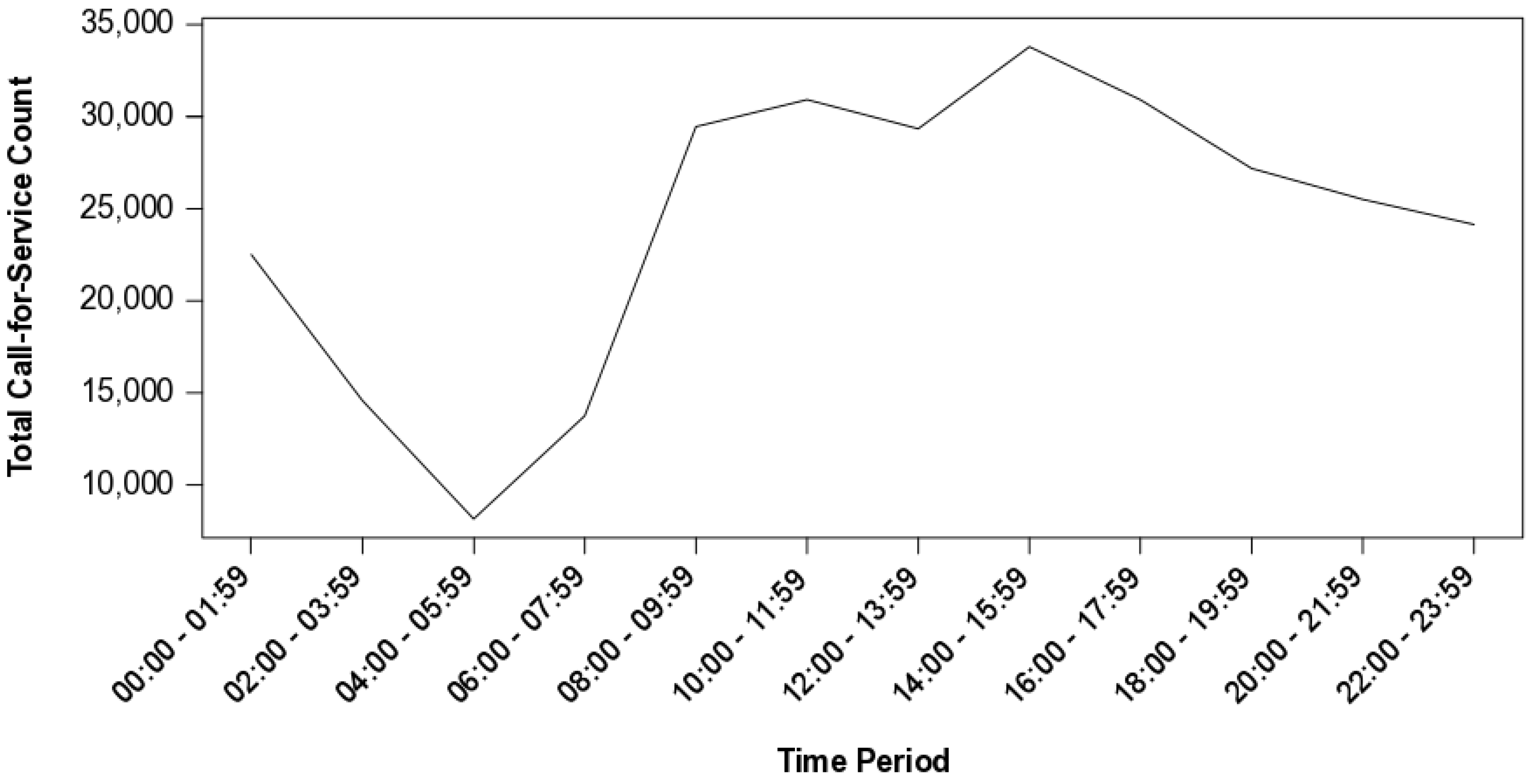
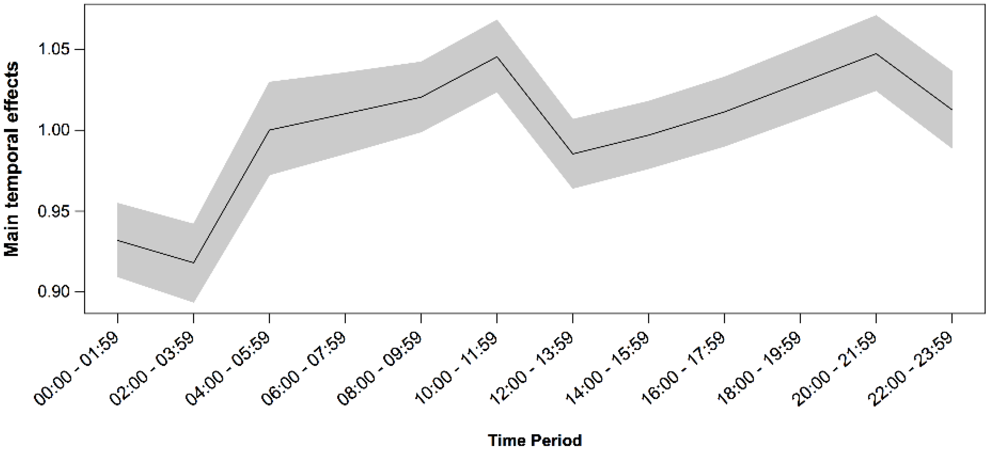
5.1. Main Temporal Effects

Main temporal effects are shown in Figure 4 and were lowest in the early morning between 02:00 and 03:59 (0.918, 95% CI: 0.894, 0.942) and highest in the evening between 20:00 and 21:59 (1.047, 95% CI: 1.025, 1.071). There was an increasing trend from early morning to the middle of the day, peaking at 10:00–11:59 (1.045, 95% CI: 1.024, 1.068), followed by a decrease at 12:00–13:59 and a gradual increasing trend through the evening. This temporal pattern is noticeably different from the observed data, where the highest number of calls-for-service occurred between 14:00 and 15:59. This can be attributed to the ICAR smoothing imposed on φ_t as well as the simultaneous analysis of spatial variation of calls-for-service.

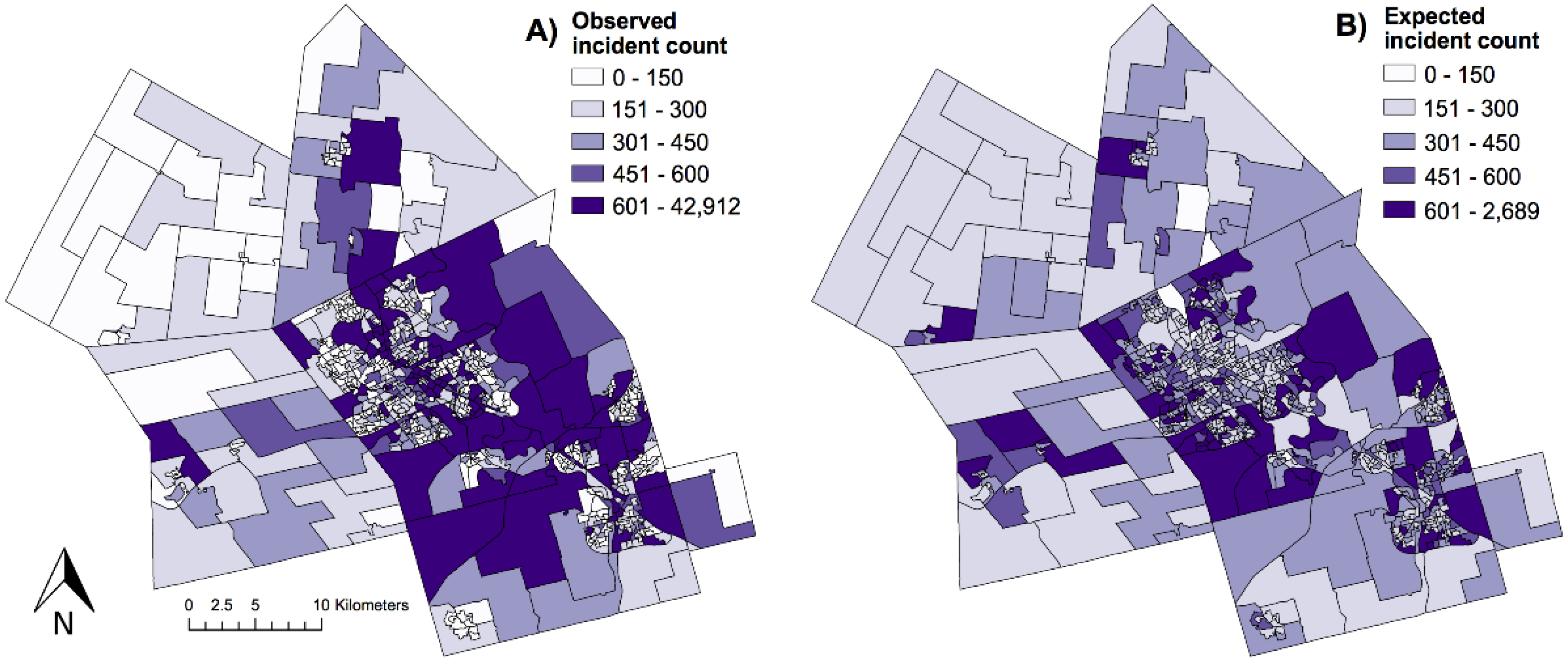
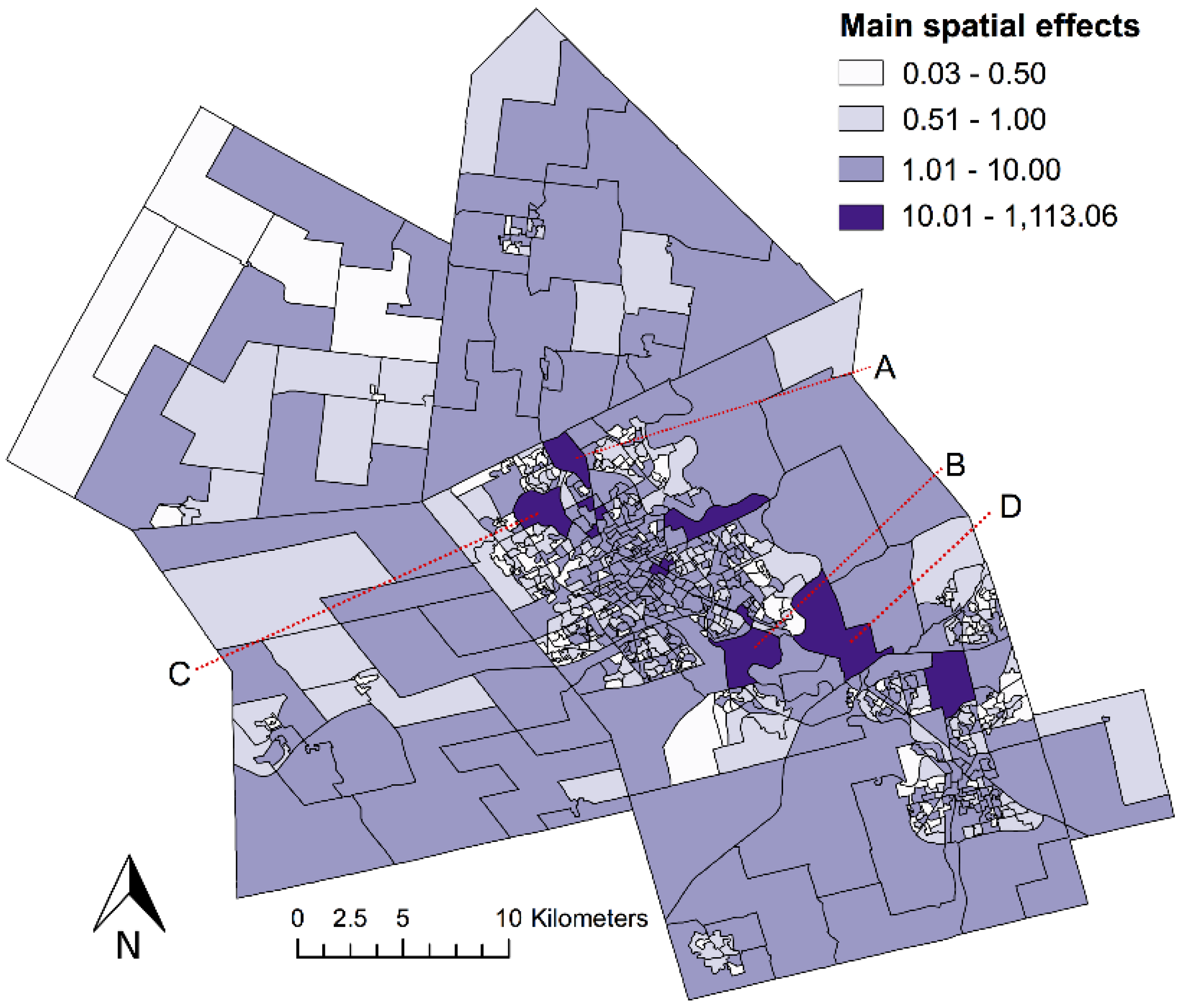
5.2. Main Spatial Effects

Main spatial effects of calls-for-service are shown in Figure 5. In general, main spatial effects were highest in central areas of the study region and lowest in peripheral and rural areas, particularly in the northwest. The highest spatial risk was found in Area A (1113.06, 95% CI: 781.77, 1551.25) which is likely due to a residential population considerably smaller than all other areas, and consequently, a low expected calls-for-service count (Figure 5). This is a limitation of using residential population to calculate expected counts. Area B had the second highest spatial risk of 284.76 (95% CI: 204.93, 388.51). The characteristics of Areas B, C, and D are relevant to understanding the geographic distribution of police calls-for-service and are discussed below.

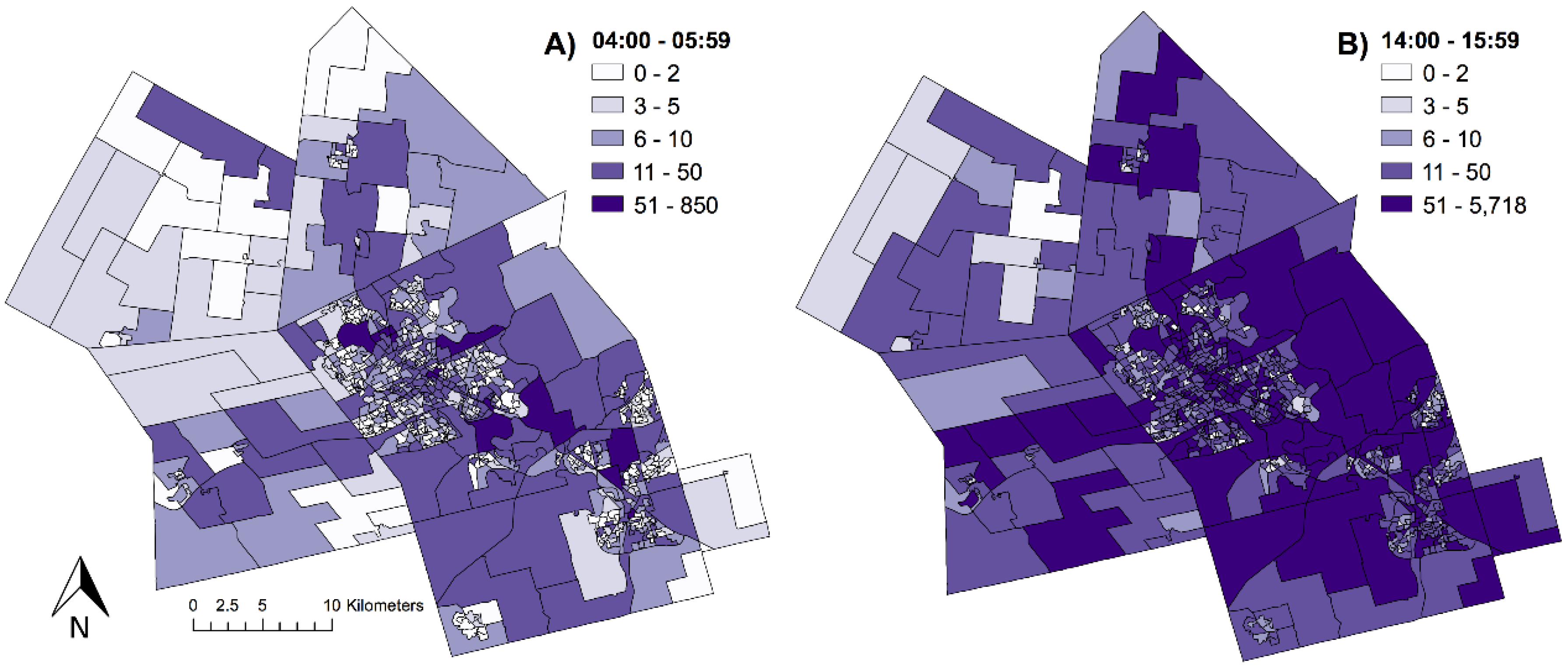
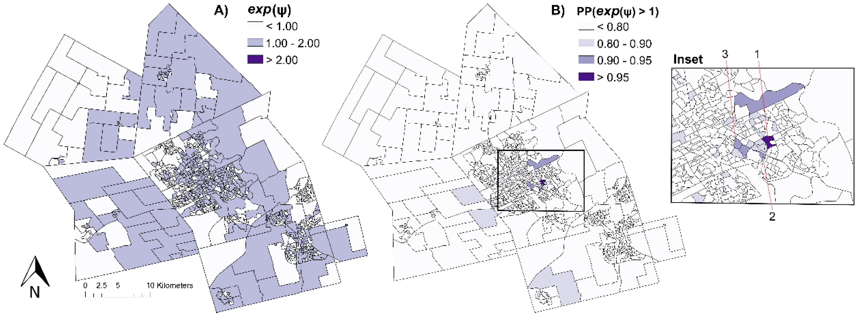
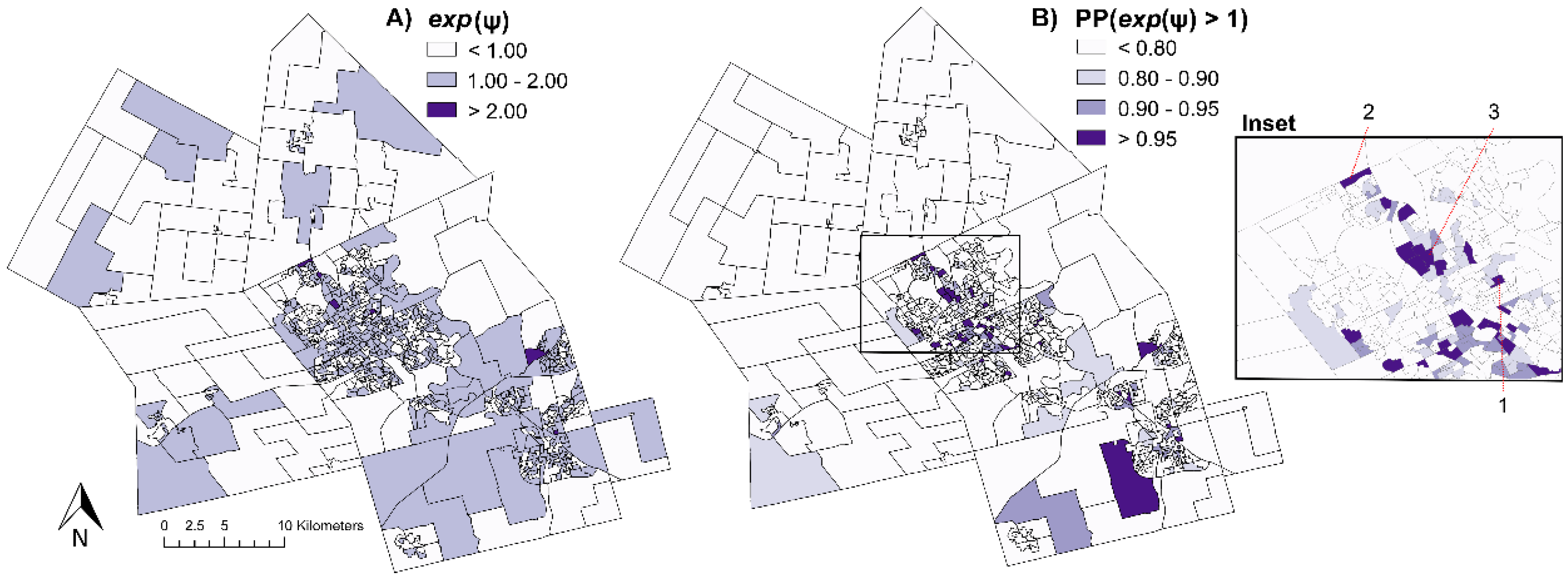
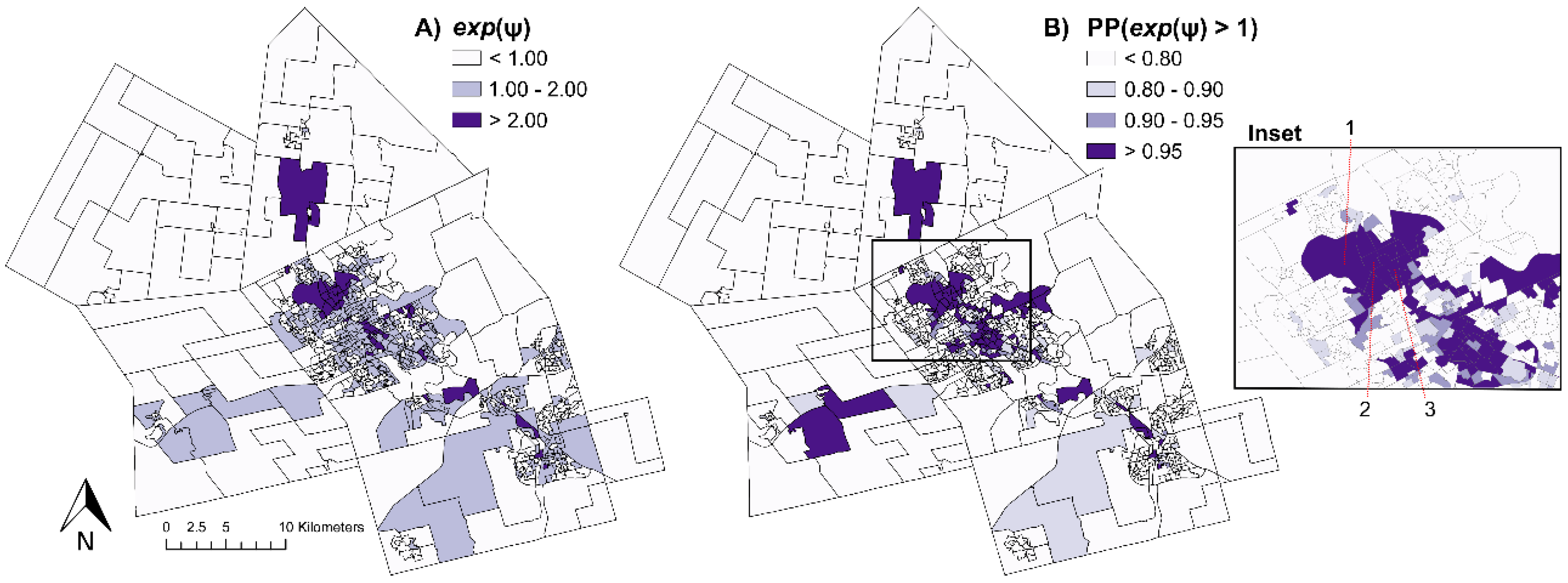
5.3. Space-Time Interaction

Space-time interaction and space-time hotspots for 10:00–11:59 and 20:00–21:59 are shown in Figure 6 and Figure 7, respectively. These time periods were chosen because they correspond to the highest main temporal effects (Figure 4) and demonstrate the geographic variability in space-time interaction throughout the course of a day. Space-time hotspots were identified by monitoring the posterior probability (PP) that exp(Ψ_it) is greater than 1. PP can be interpreted as the Bayesian equivalent of a p-value [61]. The closer PP is to 1, the stronger the evidence that areas are space-time hotspots. Compared with the point estimate (i.e., posterior mean) of space-time interaction (Ψ_it), PP is a more robust indicator for detecting hotspots since it accounts for the variance/uncertainty of Ψ_it and makes use of the full posterior probability distribution of Ψ_it, potentially minimizing the probability of detecting false hotspots [53].

6. Discussion

Results of this analysis help to understand spatial, temporal, and spatio-temporal law enforcement resource demand and provide a starting point for more detailed inquiry focused on possible explanations for space-time patterns. Providing context for the interpretation of results is the routine activity theory, which hypothesizes that crime offenses result from the convergence of motivated offenders, suitable targets, and a lack of capable guardianship in time and space [62]. While the routine activity theory was originally proposed to explain crime offenses, it has been used extensively to analyze call-for-service data because it provides a theoretical lens to interpret spatio-temporal fluctuations in police data as a function of population-level movement patterns as well as small-area land-use characteristics [63]. It should be noted that the types and quantities of police resources required when responding to different classes of calls-for-service varies and that this is one limitation of analyzing aggregated call-for-service data.

6.1. Interpreting Results of Spatio-Temporal Analysis

Main temporal effects of police calls-for-service are representative of the general shifts in resource demand throughout the course of a day and can, for example, be used to interpret overall staffing requirements. As shown in Figure 4, the main temporal effect peaks at two time periods, between 10:00 and 11:59 and between 20:00 and 21:59. Despite similar main temporal effects, the compositions of calls-for-service for these time periods were distinct. For example, there were a total of 1843 reported motor vehicle collisions during 10:00–11:59 compared to 767 during 20:00–21:59. Similarly, during 20:00–21:59 there were 1447 bylaw complaints compared to 495 during 10:00–11:59. Applied to police resource allocation, dispatch staffing should peak at these two time periods, however, higher levels of police units capable of responding to motor vehicle collisions should be staffed during 10:00–11:59 and higher levels of bylaw enforcement should be staffed during 20:00–21:59.

Main spatial effects highlight the general spatial pattern of police calls-for-service. Areas with high spatial effects have consistently high numbers of calls-for-service and are areas where police resources should be directed for all time periods. Exploring the characteristics of Areas B, C, and D provides insight into reasons these areas may have high spatial effects. The study region’s largest shopping centre and a major transit node are located in Area B and frequently occurring incidents in this area were motor vehicle stops (1108), minor motor vehicle collisions (187), and traffic enforcement (169). Area C contains a large university and student housing and incidents were largely composed of lost or damaged property (1257), general emergency calls (220), and small theft (372). Area D contains a major highway that transects the study region and calls-for-service in this area were dominated by emergency calls (38,173), incidents recorded as part of routine detail (750), and vehicle stops (459).

Space-time interaction estimates area-specific departures from main spatial and main temporal effects [44] and indicates if additional resources are needed for specific areas apart from baseline spatial and temporal resource allocations. For 10:00–11:59, there were no areas with exp(Ψ_it) > 1.5 and areas with moderate Space-time interaction were dispersed throughout the study region (Figure 6A). In comparison, during 20:00–21:59, there were 63 areas with exp(Ψ_it) > 1.5 and these areas were concentrated in and around central business areas (Figure 7A). This may be explained by the shifting patterns of routine activities of residents [62]: daytime employment and leisure activities are geographically dispersed in urban, suburban, and rural areas of the study region, while central business areas are where evening leisure activities are concentrated [64,65].

Space-time hotspots, identified by evaluating the posterior probability of exp(Ψ_it) > 1.0, are specific areas that require additional law enforcement resources to handle high numbers of calls-for-service. Posterior probability ranges from 0 to 1 and enables hotspot areas to be ranked based on the strength that exp(Ψ_it) > 1.0. The three areas with greatest PP for 10:00–11:59 and 20:00–21:59 are shown in Figure 6B and Figure 7B (labelled as Areas 1, 2, and 3), respectively. During 10:00–11:59, Space-time hotspots were found to be concentrated in the central business area of Kitchener, but located close to a local university during 20:00–21:59.

To further explore geographic variations in space-time interaction, we visualize space-time interaction and space-time hotspots for 02:00–03:59 (Figure 8A,B, respectively). This time period had the lowest main temporal effect (Figure 4). During this time period, space-time interaction was clustered around central business areas and extended along the major commercial and transportation corridor in the study region. While overall staffing may be lowest during this time period, calls-for-service were geographically clustered so that resources can be targeted to specific high-demand areas.

6.2. Modeling Bigger Spatio-Temporal Datasets with INLA

Bayesian analysis of spatio-temporal datasets via MCMC algorithms is computationally expensive because they gradually alter posterior distributions and require researchers to monitor posterior estimates and check convergence diagnostics [42]. INLA, in contrast, calculates posterior distributions through numerical integration and does not require consistent monitoring of convergence. We compared the time required to estimate Equation (3) with the simplest Type I space-time interaction on an IBM ThinkPad with a 2.4 GHz processor and 12 gigabytes RAM. Using MCMC in WinBUGS, model convergence required approximately 13 hours whereas INLA required approximately seven minutes.

While this research analyzes 9060 space-time units, the advantages of INLA modeling may be more fully realized on bigger spatio-temporal datasets. When data are available for large spatial and temporal extents, INLA spatio-temporal models may be applied to analyze small-area data for a country (e.g., Canada was composed of 56,204 DAs in 2011) over many years to identify generalizable, regional, and neighbourhood-specific patterns in calls-for-service. When spatio-temporal point data are available, INLA can be extended via stochastic differential partial equation (SPDE) modeling [40].

7. Conclusions

The implementation of computer-aided-dispatch systems in law enforcement has led to the increasing availability of call-for-service datasets with both spatial and temporal information. These datasets have facilitated the growth of crime mapping, however past research has infrequently considered spatial and temporal patterns simultaneously. Space-time analysis requires methods that can identify spatial and temporal patterns, as well as space-time interaction, and account for both local spatial autocorrelation and temporal autocorrelation.

This research applied a Bayesian spatio-temporal modeling approach implemented via INLA to identify spatial, temporal, and Space-time patterns of calls-for-service for two-hour time periods at the small-area level. Results were interpreted through the routine activity theory, which focuses on population-level activity patterns in both space and time. It was shown that main temporal effects of calls-for-service peaked between 20:00 and 21:59 and were lowest between 02:00 and 03:59. Purely spatial call-for-service patterns showed high risk in central business areas and in areas with highways, a local university, and a regional shopping centre. Space-time interaction estimates departures from main spatial and temporal patterns and enables the identification of space-time hotspots, or areas with high posterior probability of exhibiting space-time interaction greater than 1. During daytime hours (10:00–11:59), space-time hotspots were dispersed throughout the study region but during evening (20:00–21:59) and early morning time periods (02:00–03:59) space-time hotspots were clustered in downtown areas and close to a local university.

One limitation of this research is that expected call-for-service counts were calculated using residential population. Recent research has shown that alternative measures of population (i.e., the denominator in crime rate calculations) may influence the results and interpretation of spatial analyses of crime [66]. Future research may consider including alternative measures to population, such as ambient populations, workday or commuting populations, or populations estimated via social media data [67]. A second limitation of this research is that we only consider the routine activity theory and that there are a variety of additional theoretical perspectives and covariates not included. Future studies analyzing a specific call-for-service type should include covariates such as neighbourhood socioeconomic status, local land-use composition, and police perception, particularly if analyzing specific types of calls-for-service [6,68]. Analysis of specific call types may also provide more details regarding the types and quantities of law enforcement resources required.

Future research analyzing spatio-temporal datasets should consider analyzing service time (i.e., hours of law enforcement resources) to better understand overall resource allocation and match call-for-service data to service time to quantify the resources required by different call types. While this research described the spatial, temporal, and residual spatio-temporal patterns of crime, small-area risk factors were not included. Future research should explore associations between neighbourhood characteristics and calls-for-service by extending this spatio-temporal model to include covariates and consider analyzing point data to highlight specific addresses or intersections where calls-for-service exhibit high clustering [62]. It would also be advantageous to analyze hourly patterns in context of daily, monthly, and seasonal patterns, which may be suited for a multilevel spatio-temporal modeling approach. Finally, future research may adapt the presented spatio-temporal Bayesian model for probabilistic forecasts [69,70].

References

1. Chan, J.B.L. The technological game: How information technology is transforming police practice. Criminol. Crim. Justice 2001, 1, 139–159. [Google Scholar] [CrossRef]
2. Sanders, C.B.; Hannem, S. Policing “the risky”: Technology and surveillance in everyday patrol work. Can. Rev. Sociol. 2012, 49, 389–410. [Google Scholar] [CrossRef]
3. Manning, P.K. Information technologies and the police. Crime Justice 1992, 15, 349–398. [Google Scholar] [CrossRef]
4. Bursik, R.J.; Grasmick, H.G. The use of multiple indicators to estimate crime trends in American cities. J. Crim. Justice 1993, 21, 509–516. [Google Scholar] [CrossRef]
5. Manning, P.K. Technology’s ways: Information technology, crime analysis and the rationalizing of policing. Criminol. Crim. Justice 2001, 1, 83–103. [Google Scholar] [CrossRef]
6. Klinger, D.A.; Bridges, G.S. Measurement error in calls-for-service as an indicator of crime. Criminology 1997, 35, 705–726. [Google Scholar] [CrossRef]
7. Quick, M.; Law, J. Exploring hotspots of drug offences in Toronto: A comparison of four local spatial cluster detection methods. Can. J. Criminol. Crim. Justice 2013, 55, 215–238. [Google Scholar] [CrossRef]
8. Craglia, M.; Haining, R.; Wiles, P. A comparative evaluation of approaches to urban crime pattern analysis. Urban Stud. 2000, 37, 711–729. [Google Scholar] [CrossRef]
9. Murray, A.T.; Mcguffog, I.; Western, J.S.; Mullins, P. Exploratory spatial data analysis techniques for examining urban crime. Br. J. Criminol. 2001, 41, 309–329. [Google Scholar] [CrossRef]
10. Ceccato, V. Homicide in São Paulo, Brazil: Assessing spatial-temporal and weather variations. J. Environ. Psychol. 2005, 25, 307–321. [Google Scholar] [CrossRef]
11. Nakaya, T.; Yano, K. Visualising crime clusters in a space-time cube: An exploratory data-analysis approach using space-time kernel density estimation and scan statistics. Trans. GIS 2010, 14, 223–239. [Google Scholar] [CrossRef]
12. Shiode, S. Street-level spatial scan statistic and STAC for analysing street crime concentrations. Trans. GIS 2011, 15, 365–383. [Google Scholar] [CrossRef]
13. Andresen, M.A. Testing for similarity in area-based spatial patterns: A nonparametric Monte Carlo approach. Appl. Geogr. 2009, 29, 333–345. [Google Scholar] [CrossRef]
14. Weisburd, D.; Bushway, S.; Lum, C.; Yang, S.-M. Trajectories of crime at places: A longintudinal study of street segments in the city of Seattle. Criminology 2004, 42, 283–321. [Google Scholar] [CrossRef]
15. Groff, E.R.; Weisburd, D.; Yang, S.-M. Is it important to examine crime trends at a local “Micro” level? A longitudinal analysis of street to street variability in crime trajectories. J. Quant. Criminol. 2010, 26, 7–32. [Google Scholar] [CrossRef]
16. Robertson, C.; Nelson, T.A.; MacNab, Y.C.; Lawson, A.B. Review of methods for Space-time disease surveillance. Spat. Spatiotemporal. Epidemiol. 2010, 1, 105–116. [Google Scholar] [CrossRef] [PubMed]
17. Grubesic, T.H.; MacK, E.A. Spatio-temporal interaction of urban crime. J. Quant. Criminol. 2008, 24, 285–306. [Google Scholar] [CrossRef]
18. Rey, S.J.; Mack, E.A.; Koschinsky, J. Exploratory space-time analysis of burglary patterns. J. Quant. Criminol. 2012, 28, 509–531. [Google Scholar] [CrossRef]
19. Warner, B.D.; Pierce, G.L. Reexamining social disorganization theory using calls to the police as a measure of crime. Criminology 1993, 31, 493–517. [Google Scholar] [CrossRef]
20. Craglia, M.; Haining, R.; Signoretta, P. Modelling high-intensity crime areas in english cities. Urban Stud. 2001, 38, 1921–1941. [Google Scholar] [CrossRef]
21. McCord, E.S.; Ratcliffe, J.H. A micro-spatial analysis of the demographic and criminogenic environment of drug markets in Philadelphia. Aust. N. Z. J. Criminol. 2007, 40, 43–63. [Google Scholar] [CrossRef]
22. Braga, A.A.; Bond, B.J. Policing crime and disorder hotspots: A randomized controlled trial. Criminology 2008, 46, 577–607. [Google Scholar] [CrossRef]
23. Marshall, R.J. A review of methods for the statistical analysis of spatial patterns of disease. J. R. Stat. Soc. Ser. A Stat. Soc. 1991, 154, 421–441. [Google Scholar] [CrossRef]
24. Johnson, S.D.; Bowers, K.J. The stability of space-time clusters of burglary. Br. J. Criminol. 2004, 44, 55–65. [Google Scholar] [CrossRef]
25. Mburu, L.; Helbich, M. Communities as neighborhood guardians: A spatio-temporal analysis of community policing in nairobi’s suburbs. Appl. Spat. Anal. Policy 2015, 1–22. [Google Scholar] [CrossRef]
26. Li, S.; Dragicevic, S.; Castro, F.A.; Sester, M.; Winter, S.; Coltekin, A.; Pettit, C.; Jiang, B.; Haworth, J.; Stein, A.; et al. Geospatial big data handling theory and methods: A review and research challenges. ISPRS J. Photogramm. Remote Sens. 2015, 115, 119–133. [Google Scholar] [CrossRef] [Green Version]
27. Chun, Y. Analyzing space-time crime incidents using eigenvector spatial filtering: An application to vehicle burglary. Geogr. Anal. 2014, 46, 165–184. [Google Scholar] [CrossRef]
28. Blangiardo, M.; Cameletti, M.; Baio, G.; Rue, H. Spatial and spatio-temporal models with R-INLA. Spat. Spatiotemporal. Epidemiol. 2013, 7, 39–55. [Google Scholar] [CrossRef] [PubMed]
29. Besag, J.; York, J.; Mollie, A. Bayesian image restoration, with two applications in spatial statistics. Ann. Inst. Stat. Math. 1991, 43, 1–20. [Google Scholar] [CrossRef]
30. Congdon, P. Monitoring suicide mortality: A bayesian approach. Eur. J. Popul. 2000, 16, 251–284. [Google Scholar] [CrossRef]
31. Gruenewald, P.J.; Ponicki, W.R.; Remer, L.G.; Waller, L.A.; Zhu, L.; Gorman, D.M. Mapping the spread of methamphetamine abuse in california from 1995 to 2008. Am. J. Public Health 2013, 103, 1262–1270. [Google Scholar] [CrossRef] [PubMed]
32. Cerda, M.; Messner, S.F.; Tracy, M.; Vlahov, D.; Goldmann, E.; Tardiff, K.J.; Galea, S. Investigating the effect of social changes on age-specific gun-related homicide rates in New York City during the 1990s. Am. J. Public Health 2010, 100, 1107–1115. [Google Scholar] [CrossRef] [PubMed]
33. Luan, H.; Law, J.; Quick, M. Identifying food deserts and swamps based on relative healthy food access: A spatio-temporal Bayesian approach. Int. J. Health Geogr. 2015, 14, 37. [Google Scholar] [CrossRef] [PubMed]
34. Zhu, L.; Waller, L.A.; Ma, J. Spatial-temporal disease mapping of illicit drug abuse or dependence in the presence of misaligned ZIP codes. GeoJournal 2013, 78, 463–474. [Google Scholar] [CrossRef] [PubMed]
35. Law, J.; Quick, M.; Chan, P. Bayesian spatio-temporal modeling for analysing local patterns of crime over time at the small-area level. J. Quant. Criminol. 2013, 30, 57–78. [Google Scholar] [CrossRef]
36. Quick, M.; Law, J.; Luan, H. The Influence of on-premise and off-premise alcohol outlets on reported violent crime in the region of Waterloo, Ontario: Applying Bayesian spatial modeling to inform land use planning and policy. Appl. Spat. Anal. Policy 2016. [Google Scholar] [CrossRef]
37. Richardson, S.; Abellan, J.J.; Best, N. Bayesian spatio-temporal analysis of joint patterns of male and female lung cancer risks in Yorkshire (UK). Stat. Methods Med. Res. 2006, 15, 385–407. [Google Scholar] [CrossRef] [PubMed]
38. Abellan, J.J.; Richardson, S.; Best, N. Use of space time models to investigate the stability of patterns of disease. Environ. Health Perspect. 2008, 116, 1111–1119. [Google Scholar] [CrossRef] [PubMed]
39. Best, N.; Richardson, S.; Thomson, A. A comparison of Bayesian spatial models for disease mapping. Stat. Methods Med. Res. 2005, 14, 35–59. [Google Scholar] [CrossRef] [PubMed]
40. Blangiardo, M.; Cameletti, M. Spatial and Spatio-Temporal Bayesian Models with R-INLA; John Wiley & Sons: West Sussex, UK, 2015. [Google Scholar]
41. Banerjee, S.; Carlin, B.P.; Gelfand, A.E. Hierarchical Modeling and Analysis for Spatial Data, 2nd ed.; CRC Press: Boca Raton, FL, USA, 2014. [Google Scholar]
42. Carroll, R.; Lawson, A.B.; Faes, C.; Kirby, R.S.; Aregay, M.; Watjou, K. Comparing INLA and OpenBUGS for hierarchical Poisson modeling in disease mapping. Spat. Spatiotemporal. Epidemiol. 2015, 14–15, 45–54. [Google Scholar] [CrossRef] [PubMed]
43. Rue, H.; Martino, S. Approximate Bayesian inference for latent Gaussian models by using integrated nested Laplace approximations. J. R. Stat. Soc. Ser. B Stat. Methodol. 2009, 71, 319–392. [Google Scholar] [CrossRef]
44. Knorr-Held, L. Bayesian modelling of inseparable space-time variation in disease risk. Stat. Med. 1999, 19, 2555–2567. [Google Scholar] [CrossRef]
45. Felson, M.; Poulsen, E. Simple indicators of crime by time of day. Int. J. Forecast. 2003, 19, 595–601. [Google Scholar] [CrossRef]
46. Statistics Canada Dissemination Area (DA). Available online: http://www12.statcan.gc.ca/census-recensement/2011/ref/dict/geo021-eng.cfm (accessed on 17 April 2015).
47. Skogan, W.G. Efficiency and effectiveness in big-city police departments. Public Adm. Rev. 1976, 36, 278–286. [Google Scholar] [CrossRef]
48. Waterloo Regional Police Service Appendix C: WRPS 9000 Call Types. Available online: http://www.wrps.on.ca/inside-wrps/corporate-planning-systems (accessed on 6 April 2016).
49. Law, J.; Chan, P.W. Monitoring residual spatial patterns using Bayesian hierarchical spatial modelling for exploring unknown risk factors. Trans. GIS 2011, 15, 521–540. [Google Scholar] [CrossRef]
50. Lawson, A.B. Bayesian Disease Mapping: Hierarchical Modelling in Spatial Epidemiology, 1st ed.; CRC Press: Boca Raton, FL, USA, 2009. [Google Scholar]
51. Bernardinelli, L.; Clayton, D.; Pascutto, C.; Montomoli, C.; Ghislandi, M.; Songini, M. Bayesian analysis of space-time variation in disease risk. Stat. Med. 1995, 14, 2433–2443. [Google Scholar] [CrossRef] [PubMed]
52. Haining, R.; Law, J.; Griffith, D. Modelling small area counts in the presence of overdispersion and spatial autocorrelation. Comput. Stat. Data Anal. 2009, 53, 2923–2937. [Google Scholar] [CrossRef]
53. Richardson, S.; Thomson, A.; Best, N.; Elliott, P. Interpreting posterior relative risk estimates in disease-mapping studies. Environ. Health Perspect. 2004, 112, 1016–1025. [Google Scholar] [CrossRef] [PubMed]
54. Schrodle, B.; Held, L. Spatio-temporal disease mapping using INLA. Environmetrics 2011, 22, 725–734. [Google Scholar] [CrossRef]
55. Choi, J.; Lawson, A.B.; Cai, B.; Hossain, M.M. Evaluation of Bayesian spatiotemporal latent models in small area health data. Environmetrics 2011, 22, 1008–1022. [Google Scholar] [CrossRef] [PubMed]
56. Kelsall, J.E.; Wakefield, J.C. Discussion of: Best, N.G.; Arnold, R.A.; Thomas, A.; Waller, L.A.; Conlon, E.M. Bayesian models for spatially correlated disease and exposure data. In Bayesian Statistics 6; Bernardo, J.M., Berger, J.O., Dawid, A.P., Eds.; Oxford University Press: Oxford, UK, 1999; pp. 131–156. [Google Scholar]
57. Spiegelhalter, D.J.; Best, N.G.; Carlin, B.P.; van der Linde, A. Bayesian measures of model complexity and fit. J. R. Stat. Soc. Ser. B Stat. Methodol. 2002, 64, 583–616. [Google Scholar] [CrossRef]
58. Congdon, P. Applied Bayesian Modelling, 2nd ed.; Wiley & Sons: West Sussex, UK, 2014. [Google Scholar]
59. Cowles, M.K. Model comparison, model checking, and hypothesis testing. In Applied Bayesian Statistics: With R and OpenBUGS Examples; Springer Texts in Statistics; Springer New York: New York, NY, USA, 2013; pp. 207–224. [Google Scholar]
60. Law, J.; Haining, R. A Bayesian approach to modeling binary data: The case of high-intensity crime areas. Geogr. Anal. 2004, 36, 197–216. [Google Scholar] [CrossRef]
61. Meng, C.Y.K.; Dempster, A.P. A Bayesian approach to the multiplicity problem for significance testing with binomial data. Biometrics 1987, 43, 301–311. [Google Scholar] [CrossRef] [PubMed]
62. Cohen, L.E.; Felson, M. Social change and crime rate trends: A routine activity approach. Am. Sociol. Rev. 1979, 44, 588–608. [Google Scholar] [CrossRef]
63. Sherman, L.W.; Gartin, P.R.; Buerger, M.E. Hot spots of predatory crime: Routine activities and the criminology of place. Criminology 1989, 27, 27–56. [Google Scholar] [CrossRef]
64. Brantingham, P.J.; Brantingham, P.L. Crime pattern theory. In Environmental Criminology and Crime Analysis; Willan Publishing: Portland, OR, USA, 2008; pp. 78–93. [Google Scholar]
65. Groff, E.R.; Lockwood, B. Criminogenic facilities and crime across street segments in Philadelphia: Uncovering evidence about the spatial extent of facility influence. J. Res. Crime Delinq. 2014, 51, 277–314. [Google Scholar] [CrossRef]
66. Malleson, N.; Andresen, M.A. The impact of using social media data in crime rate calculations: Shifting hot spots and changing spatial patterns. Cartogr. Geogr. Inf. Sci. 2015, 42, 112–121. [Google Scholar] [CrossRef]
67. Malleson, N.; Andresen, M.A. Exploring the impact of ambient population measures on London crime hotspots. J. Crim. Justice 2016, 46, 52–63. [Google Scholar] [CrossRef]
68. Hagan, J.; Gillis, A.R.; Chan, J. Explaining official delinquency: A spatial study of class, conflict, and control. Sociol. Q. 1978, 19, 286–398. [Google Scholar] [CrossRef]
69. Cohen, J.; Gorr, W.L.; Olligschlaeger, A.M. Leading indicators and spatial interactions: A crime-forecasting model for proactive police deployment. Geogr. Anal. 2007, 39, 105–127. [Google Scholar] [CrossRef]
70. Fitterer, J.L.; Nelson, T.A. A review of the statistical and quantitative methods used to study alcohol-attributable crime. PLoS ONE 2015, 10, 1–24. [Google Scholar] [CrossRef] [PubMed]
Figure 1. Geographic distribution of (A) count of all police calls-for-service in 2011 and (B) expected count of calls-for-service.
Ijgi 05 00162 g001
Figure 2. Total calls-for-service by 2 hour time period.
Ijgi 05 00162 g002
Figure 3. Geographic distribution of police calls-for-service counts for (A) 04:00–05:59 and (B) 14:00–15:59.
Ijgi 05 00162 g003
Figure 4. Main temporal effects (= exp(γt + φt)) for calls-for-service. Grey indicates 95% credible interval (CI).
Ijgi 05 00162 g004
Figure 5. Main spatial effects (= exp(ui + si)) of police calls-for-service.
Ijgi 05 00162 g005
Figure 6. For 10:00–11:59, (A) space-time interaction and (B) space-time hotspots.
Ijgi 05 00162 g006
Figure 7. For 20:00–21:59, (A) space-time interaction and (B) space-time hotspots.
Ijgi 05 00162 g007
Figure 8. For 02:00–03:59, (A) space-time interaction and (B) space-time hotspot probability.
Ijgi 05 00162 g008