Article

Using Remote Sensing Products to Identify Marine Association Patterns in Factors Relating to ENSO in the Pacific Ocean

1
Key Laboratory of Digital Earth Science, Institute of Remote Sensing and Digital Earth, Chinese Academy of Sciences, Beijing 100094, China
2
Key Laboratory of the Earth Observation, Sanya 572029, Hainan, China
*
Authors to whom correspondence should be addressed.
ISPRS Int. J. Geo-Inf. 2017, 6(1), 32; https://0-doi-org.brum.beds.ac.uk/10.3390/ijgi6010032
Submission received: 9 October 2016 / Revised: 16 January 2017 / Accepted: 18 January 2017 / Published: 23 January 2017

Abstract

:
El Niño–Southern Oscillation (ENSO) and its relationships with marine environmental parameters comprise a very complicated and interrelated system. Traditional spatiotemporal techniques face great challenges in dealing with which, how, and where the marine environmental parameters in different zones help to drive, and respond to, ENSO events. Remote sensing products covering a 15-year period from 1998 to 2012 were used to quantitatively explore these patterns in the Pacific Ocean (PO) by a prevail quantitative association rule mining algorithm, that is, a priori, within a mining framework. The marine environmental parameters considered were monthly anomaly of sea surface chlorophyll-a (CHLA), monthly anomaly of sea surface temperature (SSTA), monthly anomaly of sea level anomaly (SLAA), monthly anomaly of sea surface precipitation (SSPA), and monthly anomaly of sea surface wind speed (WSA). Four significant discoveries are found, namely: (1) Association patterns among marine environmental parameters and ENSO events were found primarily in five sub-regions of the PO: the western PO, the central and eastern tropical PO, the middle of the northern subtropical PO, offshore of the California coast, and the southern PO; (2) In the western and the middle and east of the equatorial PO, the association patterns are more complicated than other regions; (3) The following factors were found to be predicators of and responses to La Niña events: abnormal decrease of SLAA and WSA in the east of the equatorial PO, abnormal decrease of SSPA and WSA in the middle of the equatorial PO, abnormal decrease of SSTA in the eastern and central tropical PO, and abnormal increase of SLAA in the western PO; (4) Only abnormal decrease of CHLA in the middle of the equatorial PO was found to be a predicator of and response to El Niño events. These findings will help to improve our abilities to identify the marine association patterns in factors relating to ENSO events.

1. Introduction

Marine association pattern refers to an association relationship with a direction among two and more marine environmental parameters. In views of marine environmental parameters, the Pacific Ocean (PO) encompasses several important regions, e.g., the western Pacific warm pool and the equatorial Pacific cold tongue, the western Pacific “rain pool” and marine desert in precipitation [1], the North Pacific Subtropical Gyre (earth’s largest contiguous biome) and the marine biological desert [2,3]. Because of its location and size, the PO plays a significant role not only in regional sea–air interaction but also in global climate change. In fact, reliable prediction always depends on a better understanding of the marine dynamics that influence the PO [4,5,6,7].
One such system is El Niño–Southern Oscillation (ENSO), a cycle of alternating warm events, called El Niño, and cold events, called La Niña [8]. ENSO is a typical signal of global climate variability that affects a variety of marine environmental parameters. They include sea surface temperature (SST), sea level anomaly (SLA), sea surface chlorophyll-a (CHL), sea surface wind (SSW), and sea surface precipitation (SSP). Together, they comprise a very complicated and interrelated system [8,9,10]. The basic properties of ENSO are zonal displacement of the western Pacific warm pool and atmospheric convection [11,12]. In combination with abnormal trade winds and atmospheric advection, they result in an abnormal increase in precipitation in the western PO, and an abnormal decrease in precipitation in the equatorial PO [13]. Through the dynamic processes, SSTs drop in the central Pacific, east–west SST gradients increase, and Equatorial trades strengthen, which leads to the spatiotemporal distribution of the upper mixed layer, thermocline, and nutrients; this distribution indirectly dominates primary productivity and spatiotemporal changes in CHL concentration [14,15]. Within the complicated and interrelated system—which marine parameters, where and how, simultaneously, respond to and drive ENSO events—is a scientific problem, that needs further study. In this manuscript, an abnormal variation means a variation relative to an averaged status during a specified long-term series, e.g., monthly, seasonal, and annual abnormal variations.
Multiple remote sensing sensors are the important sources providing the continuous and consistent set of information about the land and ocean [16], and offer new opportunities for monitoring their changes and understanding their associated relationships [7,17,18,19]. Previous studies have analyzed environmental parameters alongside ENSO events using statistical analysis and empirical orthogonal decomposition with multiple remote sensing products. For example, Curtis et al. [13] found a positive correlation relationship between extreme precipitation frequency and Niño 3.4 index in the central PO. Wu et al. [10] found that during ENSO-developing, ENSO-decaying, and normal summers, various mechanisms resulted in different rainfall–SST relations in the northwestern PO. During the ENSO event that occurred between 1997 and 1999, Wilson and Adamec [20] found four distinct biological responses in the tropical PO: (1) a symmetric off-equatorial chlorophyll increase during La Niña; (2) an equatorial decrease in chlorophyll during El Niño; (3) an off-equatorial bloom during the peak of El Niño; and, (4) a chlorophyll bloom in the western Pacific warm pool during El Niño. Park et al. [21,22] also pointed out that dominant variability of phytoplankton was associated with the ENSO, that is, during the El Niño, both an insufficient nutrient supply and a reduced surface solar radiation caused a decrease in chlorophyll; meanwhile, the chlorophyll increased the sea surface temperature and decreased the subsurface temperature by altering the penetration of solar radiation, which intensified the ENSO amplitude. Murtugudde et al. [14] evaluated the relationships among SST, sea surface height, wind speed, and mixed-layer depth to analyze the reasons for these responses. Co-variability between SST and SLA in the north PO was analyzed, and three distinct SST–SLA states were dominated by the ENSO, Pacific Decadal Oscillation and Pacific–North American patterns [23]. It was also found that during the warm phase of ENSO, the positive SST and negative sea level pressure co-occurred in the eastern tropical PO [24]. Each of these studies showed interrelation between variations in marine environmental parameters and in the relations of those parameters with ENSO.
Considering these studies alongside global climate change, the benefits of examining the interrelations among all the marine environmental parameters help in understanding the ENSO process and oceanic dynamics. Recently, the study of marine systems has been facilitated by advanced earth observation technologies, which makes acquiring lengthy time series of marine bio-optical, namely, CHL, and dynamic parameters, that is, SST, SSP, SLA, WS (wind speed), etc., from multiple remote sensing products possible [13,18,20,25]. As these studies strongly depended on the interrelation between variations in marine environmental parameters, challenges remain in discovering the marine spatiotemporal association patterns among three or more elements within a uniform framework, especially using remote sensing products on a global scale [26]. However, our previous study has examined the association patterns among marine environmental parameters using remote sensing products, and discussed their relationships with ENSO. These relationships mainly covered the three predefined regions within the northwestern PO, and such predefined regions were limited to exploring their physical process. Also, the relationships related to ENSO events need further study in the entire PO to address their physical dynamics [27].
Thus, the scientific issue of this manuscript explores which, how, and where the marine environmental parameters in different zones help to drive, and respond to, ENSO events, and to identify the marine sensitive factors to ENSO events. Traditional spatiotemporal techniques, for example, empirical component analysis, mathematical statistics, modal analysis, canonical analysis, and teleconnection analysis, are mainly limited to one to two marine parameters, and are less detailed and informative in the quantitative interrelationships [28,29,30]. That is, these methods face great challenges in dealing with the scientific issue. For dealing with the spatial relationships among ENSO and marine environmental parameters within a uniform framework, association rule mining techniques show more perspective than traditional analysis. Association rule mining techniques put multiple geographical parameters into one analyzing framework, and then obtain their association patterns simultaneously [16,26]. These techniques are typically inductive, as opposed to deductive, in that they are not used to prove or disprove pre-existing hypotheses, but rather are used to identify patterns embedded in data, and thereby support hypothesis generation [15]. Association rule mining techniques have been widely used to obtain the interrelationships among geographical parameters, including the interrelationship between bird species richness and geographical parameters [31], the spatial distribution of aerosol optical depth and its affecting factors [32], the spatial co-location patterns between the fish distribution and marine parameters [33], and the teleconnection among regional or global marine parameters [27,30,34].
The purpose of this manuscript is to quantitatively explore, using remote sensing products and within an association rule mining framework, what are those marine environmental parameters and which ones are sensitive to ENSO events. The remainder of the manuscript is organized as follows. In Section 2, the multi-marine remote sensing products and its preprocessing are introduced. In Section 3, association rule mining algorithms are presented. Section 4 summarizes the results of analysis of association patterns in the relations among marine environmental parameters and ENSO events. Section 5 discusses and interprets the results, and Section 6 presents our conclusions.

2. Remote Sensing Data Sets and Preprocessing

Considering the data acquisition capabilities from remote sensing and sensitive to global climate changes, the SST, CHL, SSP, sea surface wind speed (WS), and SLA originating from remote sensing products, and the multivariate ENSO index (MEI), were applied to explore marine association patterns. Table 1 summarizes the sources and temporal and spatial resolutions of the remote sensing products and MEI used in this research.
To obtain uniform datasets from the above remote sensing products, with the same spatial and time resolution, an analysis period of January 1998 to December 2012 was selected. The PO covering 100° E–60° W and 50° S–50° N was selected as the study area. The spatiotemporal resampling was used to generate the datasets with a spatial resolution of 1° in grid projection and with a time resolution of one month, then the monthly anomalies were calculated by removal of seasonal effects with the z-score algorithm [26,34]. The z-score algorithm took all sets of values for a given month from January to December from a long time series of products, calculated the mean and standard deviation for that set of monthly values, and then standardized each value by subtracting the mean and dividing by the standard deviation. Thus, each geographical parameter in each grid has 180 samples (15 years). The resulting anomalies were denoted as SSTA (monthly anomaly of SST), CHLA (monthly anomaly of CHL), SLAA (monthly anomaly of SLA), SSPA (monthly anomaly of SSP), and WSA (monthly anomaly of wind speed).

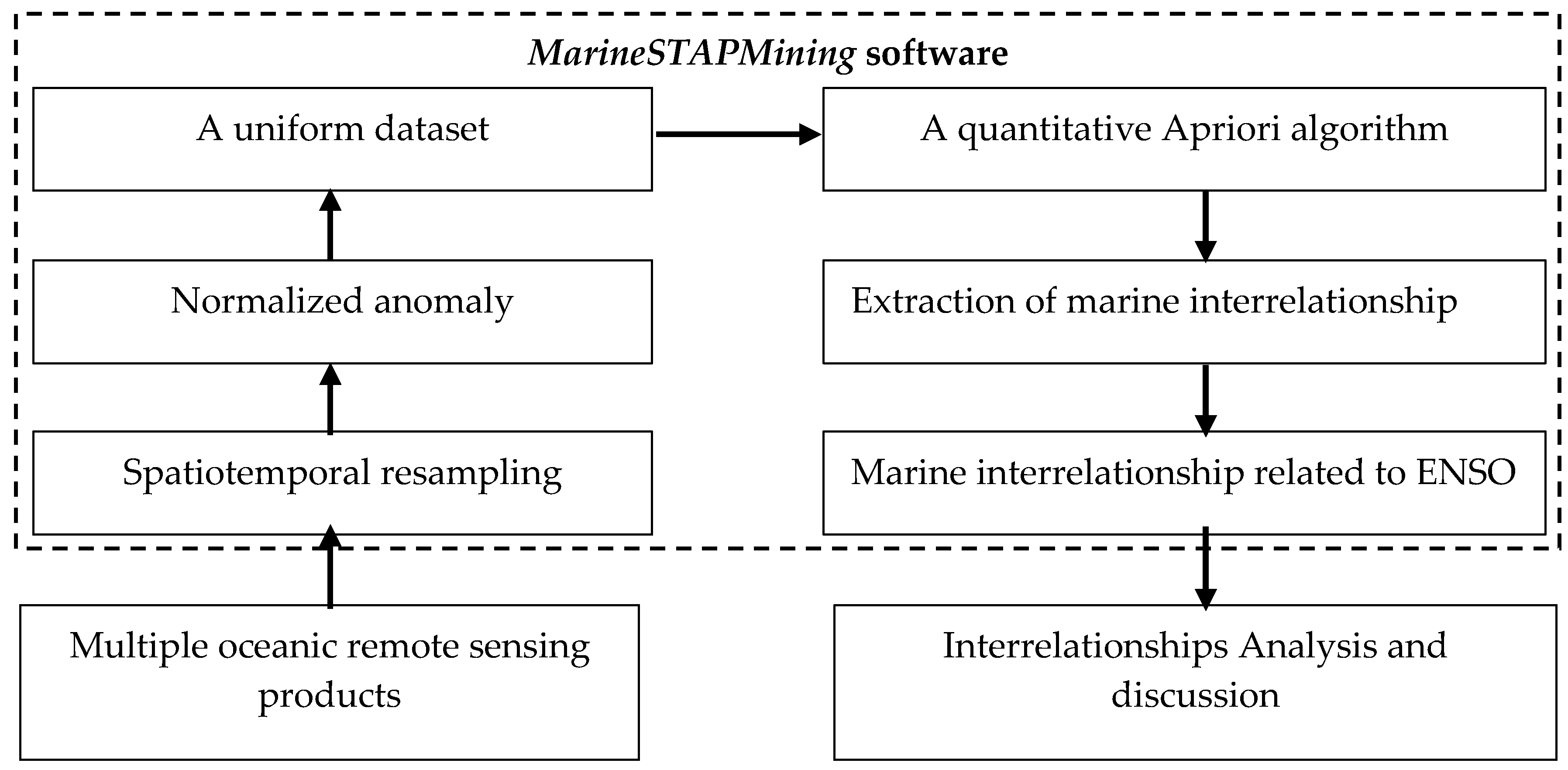
3. Quantitative Association Rule Mining with an Apriori Algorithm

After the preprocessing of normalized anomaly, the variation of geographical parameters or phenomenon will fit to normal distribution; thus, we select the standard Gaussian distribution to discretize the marine variations and ENSO index. To better identify the association patterns, standard deviations of 1 and 0.5 for the time series were used as criteria, and ENSO indices and marine environmental parameters were discretized into five ranks with a continuous interval. The five ranks are −2, −1, 0, +1 and +2. They correspond to severe negative change (not greater than −2), slight negative change (greater than −2 and not greater than −1), no change (greater than −1 and not greater than +1), slight positive change (greater than +1 and not greater than +2), severe positive change (greater than +2), respectively. On the ENSO index, −2 indicates a strong La Niña event and +2 indicates a strong El Niño event. In this manner, in normal conditions, 15.87th percentile of marine variation is regarded as severe negative/positive change and of ENSO as a strong La Niña/El Niño event, and 30.85th percentile is regarded as a slight one or a weak event.
Apriori algorithm is one of the most typical mining ones for finding association patterns, and most of the prevail mining algorithms derive from the core idea of Apriori [16,30,33,34]. To provide more information, a quantitative Apriori algorithm was used to find association patterns among marine environmental parameters and ENSO events. The inputs to the algorithm include the discretized marine parameters and ENSO events, the outputs are marine association patterns, and the processing includes two key steps [40]. The first finds frequent itemsets from the transaction mining table on the basis of recursive processing with “linking–pruning–generating,” which generates (k + 1)-dimensional candidate association rules from k-dimensional rules on the basis of the user-specified minimum thresholds. This step is repeated until no more candidate association rules are generated. The second generates an association pattern from the frequent itemsets on the basis of evaluation factors, e.g., support, confidence, lift. The quantitative association pattern is commonly represented in a form as Equation (1) [15,41].
X [ p ] Y [ q ] ( s % , c % , l )
where X is an antecedent and Y is a consequent of the association pattern (in this manuscript, either X or Y represents ENSO, and the other variable represents one and more marine environmental parameters); p and q are the quantitative levels; and s, c and l are evaluation factors representing support, confidence, and lift of the association pattern, respectively.
Support describes the probability of the co-occurrence of attributes X and Y in the dataset, which is defined as follows:
s ( X Y ) = n ( X Y ) N × 100 %
Confidence describes the probability of attribute Y occurring if attribute X occurs, defined as follows:
c ( X Y ) = s ( X Y ) s ( X ) × 100 % = n ( X Y ) n ( X ) × 100 %
Lift describes how much the occurrence of attribute X impacts the probability of the occurrence of attribute Y. Lift is defined as follows:
l ( X Y ) = n ( X Y ) n ( X ) × ( n ( Y ) N ) 1 = n ( X Y ) × N n ( X ) × n ( Y )
where n ( X ) and n ( Y ) are the number of occurrences of attributes X and Y, and n ( X Y ) is the co-occurrence of X and Y in the transaction mining table. The value N is the number of time series.
In this mining algorithm, the thresholds, namely, support, confidence and lift, are mostly dominated by users or domain experts. Different thresholds result in different association patterns. According to our experiments and statistical analysis [27,40], this manuscript sets these thresholds to 10%, 60% and 2.0, respectively, meaning that the occurring possibility of an association pattern is not less than 10% in the database, that the occurring possibility of a consequent when an antecedent occurred is not less than 60%, and that an antecedent promotes the likelihood of a consequent not less than 2.0 times. When all the s, c and l meet the user-specified thresholds, the mined association patterns are meaningful.

4. Results

The quantitative Apriori algorithm and the preprocessing of remote sensing products have been integrated into the Marine Spatiotemporal Association Patterns Mining System (MarineSTAPMining) software, which is registered by the National Copyright Administration of P.R. China (No. 2014SR013444), developed by the authors. The experimental hardware environment includes an Intel core i7 CPU at 2.80 GHz, a 500 GB hard disk, and 4.0 GB of memory. Under this computational environment, each grid pixel within the PO was discovered one by one to obtain the association patterns among marine environmental parameters and ENSO events. Only the association patterns found to have a causal relation with ENSO are discussed in this manuscript. Figure 1 shows a flowchart of this manuscript.
Each grid pixel within the raster dataset has zero to several association patterns. It was assumed that those grid pixels with more association patterns are more interactive. That is, the more the number of the association patterns in each grid pixel, the more interactive the grid pixel. According to the number of association patterns in each grid pixel and its spatial connectivity, Figure 2 is drawn. From Figure 2, five such interactive regions are found. They are the western PO (Region 1), the central and eastern tropical PO (Region 2), the middle of the northern subtropical PO (Region 3) in the North Pacific Subtropical Gyre, the middle of the southern PO (Region 4), and the region along the California coast (Region 5). The following discussions mainly focused on the five sub-regions. Thematic maps were created to depict these findings in detail. These are shown in Figure 3 and Figure 4.

4.1. Variations of Marine Environmental Parameters Inducing ENSO Occurrences

There is only one instance in which SSTA[−2]→ENSO[−2]. It is located largely in the central and eastern tropical PO, mostly covering El Niño Region 3 and Region 4 (see Figure 3a). This suggests that when SSTA drops abnormally in this region, strong La Niña events will occur. Between SSPA and ENSO, there is a positive association pattern with the forms of “SSPA[−2]→ENSO[−2]” and “SSPA[−1]→ENSO[−2]” (see Figure 3b). It covers the middle of the equatorial PO (10° S to 10° N and 160° E to 140° W) in Region 2, indicating that when SSPA drops abnormally or slightly, strong La Niña events will occur. The association pattern between SLAA and ENSO shows a positive association pattern with the form of “SLAA[−2]→ENSO[−2]” and a negative association pattern with the form of “SLAA[+2]→ENSO[−2]” (see Figure 3c). The former mainly covers the east of the equatorial PO (10° S to 10° N and 155° W to 100° W) within Region 2, meaning that when SLAA drops abnormally in this region, strong La Niña events will occur. The latter mainly displaces the western Pacific warm pool within Region 1, meaning that when SLAA rises abnormally in this region, strong La Niña events will occur. The association patterns between WSA and ENSO events (see Figure 3d) show that a positive association pattern with the forms of “WSA[−2]→ENSO[−2]” and “WSA[−1]→ENSO[−2]” occurs in the middle of the equatorial PO region (10° S to 10° N and 160° E to 150° W), meaning that when WSA in these regions drops abnormally or slightly, strong La Niña events will occur. In addition, a positive association pattern with the form of “WSA[−2]→ENSO[−2]” occurs in the east of the equatorial PO from 125° W to 95° W. Only one association pattern between CHLA and ENSO (see Figure 3e), “CHLA[−2]→ENSO[+2]” appears. It is located in a few areas in the middle of the equatorial PO, meaning that when CHLA drops abnormally, strong El Niño events will occur.

4.2. Variations in Marine Environmental Parameters Derived from ENSO Events

There are several association patterns between ENSO and SSTA (see Figure 4a), located in different regions. When a strong/weak La Niña event occurs, SSTA will drop abnormally in the central and eastern PO within Region 2 and offshore of the California coast within Region 5. The typical forms are “ENSO[−2]→SSTA[−2]” and “ENSO[−1]→SSTA[−2].” With the same events, SSTA will rise abnormally in the western PO region (10° S to 15° N and 130° E to 160° E) within Region 1 and Region 3 (28° N to 33° N and 170° E to 160° W). The typical forms are “ENSO[−2]→SSTA[+2]” and “ENSO[−1]→SSTA[+2]).” When a strong El Niño event occurs, SSTA in the middle of the equatorial PO will drop abnormally with a form of “ENSO[+2]→SSTA[−2].” When a weak El Niño event occurs, SSTA in Region 4 (50° S to 45° S and 165° W to 150° W) will rise abnormally with a form of “ENSO[+1]→SSTA[+2]).” SSTA in the Region 2 (12° S to 10° S and 160° W to 155° W) will rise slightly with a form of “ENSO[+1]→SSTA[+1]).”
The association pattern between ENSO and SSPA is shown in Figure 4b. When strong La Niña events occur, SSPA in the middle of the equatorial PO (10° S to 10° N and 160° E to 140° W) will drop abnormally or slightly with forms of “ENSO[−2]→SSPA[−2]” and “ENSO[−2]→SSPA[−1].” In addition, the relation with “ENSO[+2]→SSPA[−1]” scatters the margins of the above association patterns, meaning that when a strong El Niño event occurs, SSPA will drop slightly.
The association pattern between ENSO and WSA is shown in Figure 4c When strong La Niña events occur, WSA in the middle of the equatorial PO (150° E to 150° W) and in the east of the equatorial PO (125° W to 95° W) will drop abnormally with a form of “ENSO[−2]→WSA[−2].” However, in the middle of the equatorial PO (10° S to 8° N and 150° E to 150° W), the contradict association pattern was also found with a form of “ENSO[−2]→WSA[+2].” When weak La Niña events occur, WSA in the middle of the equatorial PO (10° S to 8° N and 150° E to 150° W) will rise abnormally with a form of “ENSO[−1]→WSA[+2].”
The association pattern between ENSO and SLAA is shown in Figure 4d. When strong La Niña events occur, SLAA in the east of the equatorial PO (10° S to 10° N and 155° W to 100° W) will drop abnormally with a form of “ENSO[−2]→SLAA [−2].” In the area of Region 4 that is offshore of New Zealand (10° S to 11° N and 120° E to 160° E), and the area of (10° S to 11° N and 120° E to 160° E) within the western Pacific warm pool, SLAA will rise abnormally with a form of “ENSO[−2]→SLAA[+2].”
The association pattern between ENSO and CHLA is shown in Figure 4e. One negative association pattern with the form of “ENSO[+2]→CHLA[−2]” covers the middle of the equatorial PO region (2° S to 2° N and 170° E to 178° W). When strong El Niño events occur, CHLA in this region will drop abnormally.

5. Discussion

In this study, the strengths of ENSO events are defined not by using traditional definitions, but based on historic data. A strong El Niño event is defined as having an MEI of more than one standard deviation, and a strong La Niña event is defined as having an MEI of less than negative one standard deviation. Except in the case of one La Niña event that occurred from October 1995 to March 1996, we categorized the strengths of ENSO events in the same manner as [42,43]. This manuscript defines the El Niño/La Niña threshold as the radio of the time length of El Niño/La Niña event occurrences divided by the length of whole time series. The threshold for an El Niño event is the 29.49th percentile, and a La Niña event, the 30.13th percentile, which almost agrees with the 30.00th given by [39]. The identified El Niño and La Niña events during the period from January 1998 to December 2012 are shown in Table 2.
Table 2 shows that during this period of January 1998 to December 2012, six El Niño events and seven La Niña events occurred. As the main cycle of ENSO is 2–7 years [8,24], the research time span of fifteen years is sufficient for investigating the characteristics of ENSO. In addition, many previous studies have documented the relationships between ENSO and marine environments and gained promising results using similar time spans [13,14,19,20,22,44].
As the thresholds, that is, support, confidence, and lift, used to find the meaningful patterns, are determined by the users’ interest, the association patterns are mostly arbitrary. To overcome the shortcoming, we carry out many experiments to find the optimal thresholds, and the support, confidence, and lift thresholds of 10.0%, 60.0% and 2.0 are more suitable in the Pacific Ocean [26]. That is to say, all the association patterns in this manuscript have a support not less than 10.0%, a confidence not less than 60.0%, and a lift not less than 2.0. As a result, we can calculate that during the period from January 1998 to December 2012, all association patterns co-occur no less than 18.0 times (the co-occurrence possibility is not less than 10.0%), and once the antecedent occurs, the occurrence of the consequent is not less than 60.0%. In addition, the former occurrence promotes the likelihood of the latter occurrence not less than 2.0 times. Under the above conditions, the discovered association patterns between marine environmental parameters and ENSO events prevail from the central and eastern tropical PO, through the western PO, to the central northern subtropical PO and the central southern PO.
As one of the strongest signals of global climate changes, ENSO will cause variations in marine environmental parameters, and these variations will relate to one another [8]. In contrast, the abnormal change in marine environmental parameters in certain regions within the PO may predict ENSO occurrences (e.g., SST in El Niño regions, SSP in the central tropical PO) [45]. To provide a fuller picture of the physical effects of these association patterns, we integrated all the association patterns between marine environmental parameters and ENSO events into an ENSO-oriented association pattern network. The association pattern network reveals different physical effects during the warm and cold phases. In this network, both the association patterns of “XY” and “YX” are true at the same time, these association patterns are defined as a mutual relationship.

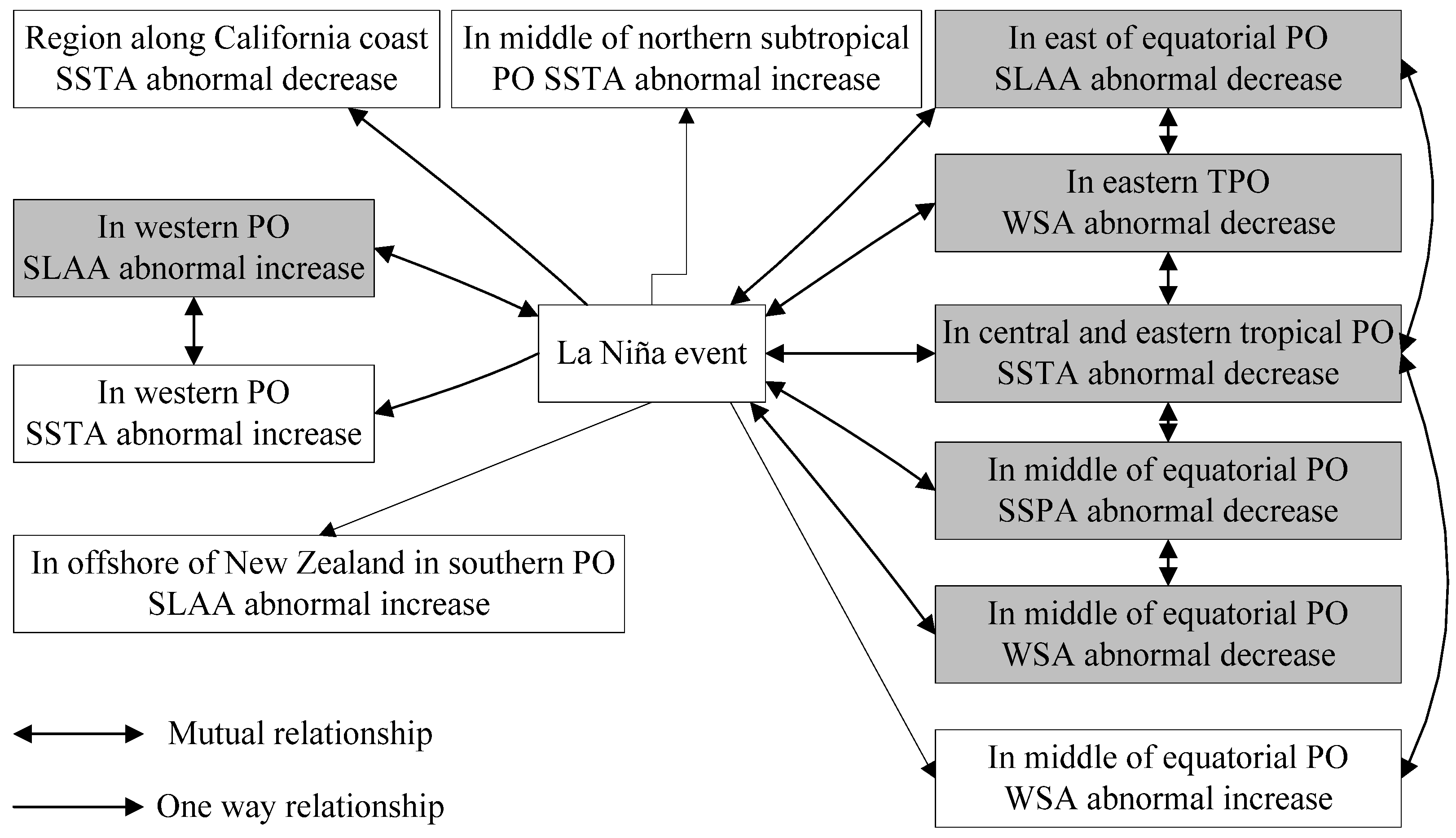
5.1. Association Patterns among La Niña Events and Marine Environmental Parameters

In normal conditions, the western PO is mostly within the western Pacific warm pool. When La Niña events occur, the westward Rossby reaches the central PO, which pushes the warm pool at the surface toward the west. The westward flow of warm water results in SSTA increasing and in decreasing water mass transport, accumulating westward, so SLAA in the western PO increases. At the same time, the SLAA’s decreasing with SSTA is located eastwards by the counteract effects of Kelvin and Rossby wave along the Equator, at the eastern boundary of the PO. SSTA in the eastern tropical PO (within Region 2) and along the California coast (Region 5) has a tendency to reduce under the influences of Eastern boundary currents such as the Peru Cold Current and the California Cold Current. SLAA decreases due to the cold upper water descending when the currents flow toward the Equator from high-latitude areas. Yu et al. [46] found the SSTA dipole along the California coast through modeling.
When La Niña events occur, the thermocline in the central Pacific becomes shallower by forcing of Rossby, the warmer water accumulates in western PO, and the colder-than-normal water in the eastern equatorial Pacific begins to develop, then the east–west SST gradient increases. This strengthens the trade winds, resulting in an abnormal increase in WSA in the eastern equatorial PO and an abnormal decrease in WSA in the central tropical PO. Under the force of trade winds and Walker circulation, the rainfall shifts westward. SSPA in the middle of the tropical PO drops abnormally by up to half of one standard deviation [13]. Curtis et al. [13] based their studies on the period from 1979 to 2004. Association patterns among La Niña events and marine environmental parameters are shown in Figure 5.
It can be seen from Figure 5 that when La Niña events occur, several effects will prevail: abnormal decrease of SLAA and WSA in the east of the equatorial PO; abnormal decrease of SSPA and WSA in the middle of the equatorial PO; abnormal decrease of SSTA in the eastern and central tropical PO; and abnormal increase of SLAA in the western PO. It can also be seen that some environmental parameters (shaded gray in Figure 5) exhibit mutual relationships with La Niña events. In these cases, when the marine environmental parameters are opposite to those outlined above, La Niña events will not occur. These association patterns indicate that abnormal changes in these parameters not only occur in response to La Niña events but also predict them.
It is also noteworthy that SSTA in the northern subtropical PO and SLAA in the southern PO are changing, which may be responses to La Niña events. When La Niña occurs, the North Pacific Current flows eastward through the middle of the northern subtropical PO, resulting in mean SST increases. Offshore of New Zealand in the southern PO, the combined influence of the Antarctic Circumpolar Current and the Subtropical Convergent Zone results in an abnormal rise in SLAA. WSA increases with decreasing SSTA in the central tropical PO because of decreased heat flux and because of water vapor transporting into the air, both of which stir the tropical atmospheric circulation.

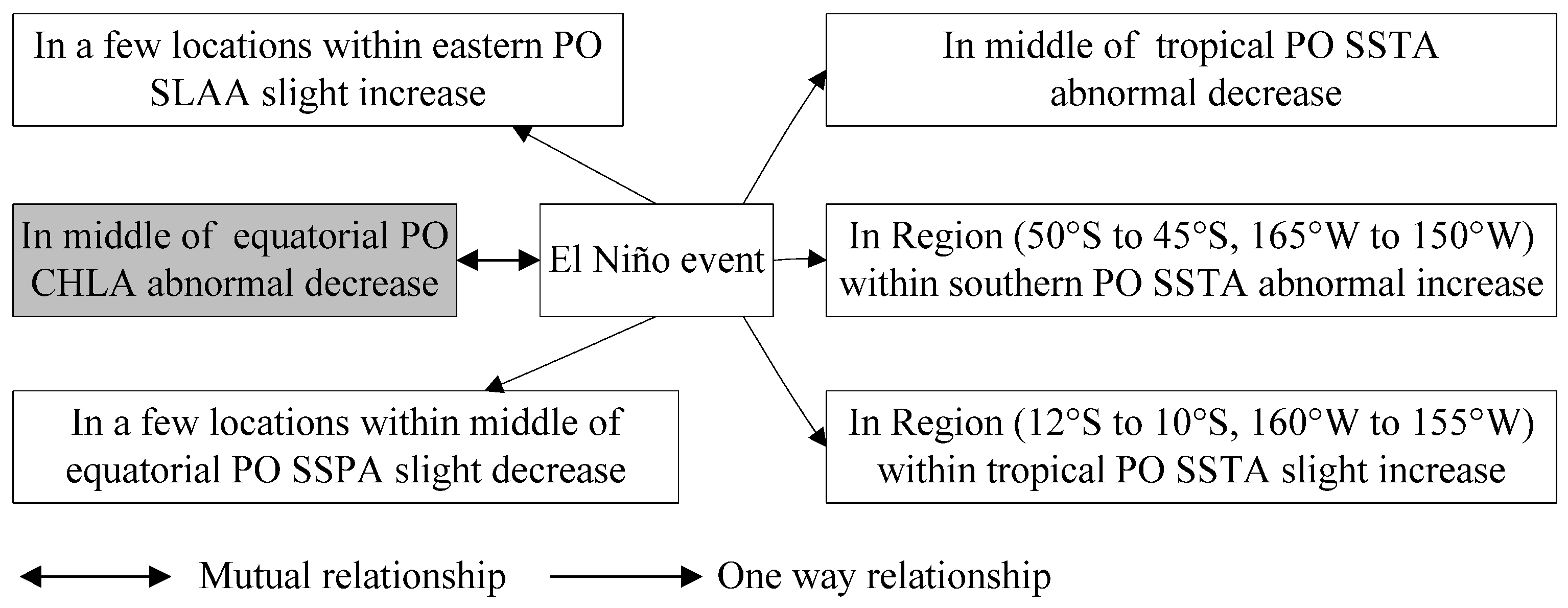
5.2. Association Patterns among El Niño Events and Marine Environmental Parameters

Association patterns among El Niño events and marine environmental parameters are shown in Figure 6. Mutual relationships are shaded in gray. Marine environmental parameters change when El Niño events occur, but these changes are not obviously related to each other. With the exception of the abnormal decrease in CHLA in the middle of the equatorial PO, no parameter can be considered an indicator of El Niño events. With the decreases of CHL, the SST decreases and the subsurface temperature increases by altering the penetration of solar radiation, deepening the mixed layer and thermocline. Such ocean states could intensify ENSO amplitude [21], thus the abnormal decrease of CHLA may be an indirect indicator of El Niño events.
Generally, once the El Niño events occur, the wind stress in the central Pacific relaxes and southeast trade winds reverse direction, which weakens the wind speed in the middle of the equatorial PO, and deepens the thermocline there. The deepening thermocline develops an eastward propagating Kelvin wave and a westward propagating Rossby wave, promoting the warmer water expanding from west to east and occupying the entire middle PO and part of the eastern tropical PO. As a result, SLAA in the eastern PO rises by up to half of one standard deviation. With the warmer water expanding eastward from the western PO, the warmer water from the eastern PO also extends westward, which results in downwelling in the middle of the equatorial PO. The downwelling and the abnormal decrease in rainfall in the same region limit the surface supply of nutrients and weaken phytoplankton growth [47]. Then, CHLA in the middle of the equatorial PO decreases abnormally by less than one standard deviation. Abnormal increases in SSTA in the southern PO (50° S to 45° S and 165° W to 150° W) during El Niño occurrences are the result of global atmospheric circulation being modified through changes created by Walker–Hadley circulation, which in turn modifies the heat flux exchanges at the sea–air interface, and induces the SST to rise [48].
Compared with La Niña events, the El Niño association pattern network is simple, and the changing characteristics of marine environments are not typical, especially in spatial regions at a large scale. As is well known, there are two types of El Niño events in the PO: central Pacific El Niño events and Eastern Pacific El Niño events. Using the Formula (1) in Ashok et al. [49], we recalculated the El Niño Modoki Index (EMI) during the period of January 1998 to December 2012, and found that the central Pacific El Niño events occur May 2002–March 2003, August 2004–May 2005, June 2006–February 2007 and June 2009–May 2010, which are consistent with the results in [19]. That is to say, four out of six are the central Pacific El Niño events, and the other two are Eastern Pacific ones. Eastern Pacific events are characterized by strong anomalous warming in the eastern equatorial Pacific, whereas, central Pacific El Niño events are associated with strong anomalous warming in the central tropical Pacific and cooling in the eastern and western tropical Pacific [49]. Associated with this distinct warming and cooling patterns, the teleconnection patterns between them are very different, which also dominate the other marine parameters [50,51].
It is also notable that in the western PO, at the descending part of the Hadley cell circulation, SLAA increases whether cold or warm events occur. The Hadley cell circulation is enhanced at the Equator during La Niña events and in the center of the tropical PO during El Niño events.

6. Conclusions

In this manuscript, we discussed data on ocean systems that were gathered using multi-marine remote sensing products during the period from January 1998 to December 2012. The data were analyzed to determine association patterns between and among the parameters and ENSO events in the PO. Compared to the previous studies, with remote sensing products, we not only obtained the well-known knowledge, but also the new-to-earth scientists. These findings help to improve our understanding of what, how and where marine environmental parameters in different zones are predicators of, and responses to, ENSO events, and also offer new ways to distinguish marine regions that are sensitive to ENSO events and new ways to define ENSO indices. The main conclusions are summarized as follows.
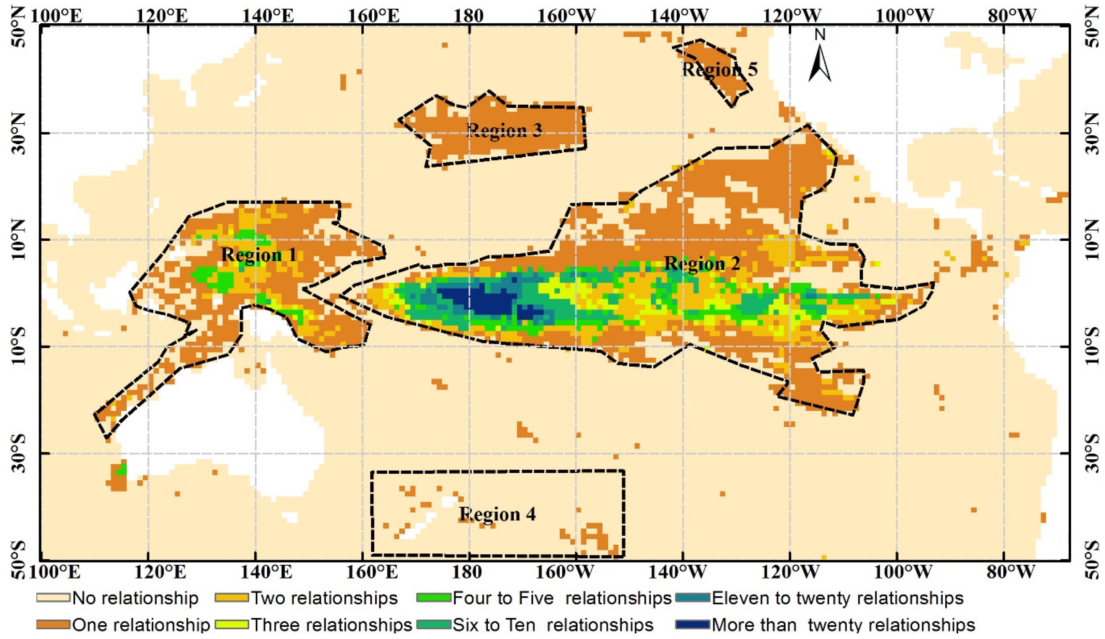
  • Association patterns among marine environmental parameters and ENSO events in the PO mainly occur in five sub-regions of the PO: the western PO, the central and eastern tropical PO, the middle of the northern subtropical PO, offshore of the California coast, and in the southern PO. In the western PO and the middle and east of the equatorial PO, the association patterns are more complicated.
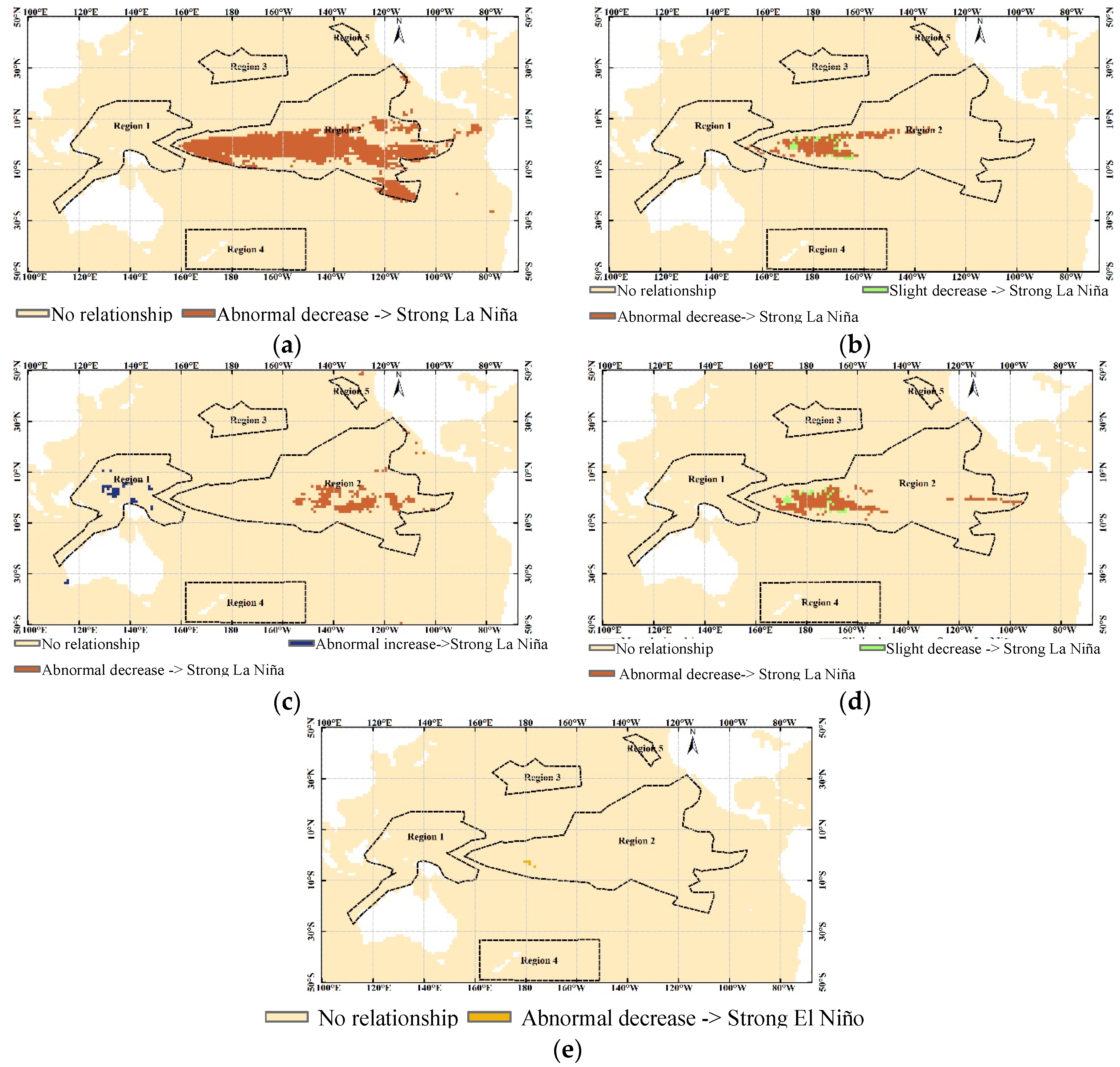
  • The following factors are considered predicators of and responses to La Niña events: abnormal decrease of SLAA and WSA in the east of the equatorial PO, abnormal decrease of SSPA and WSA in the middle of the equatorial PO, abnormal decrease of SSTA in the eastern and central tropical PO, and abnormal increase of SLAA in the western PO.
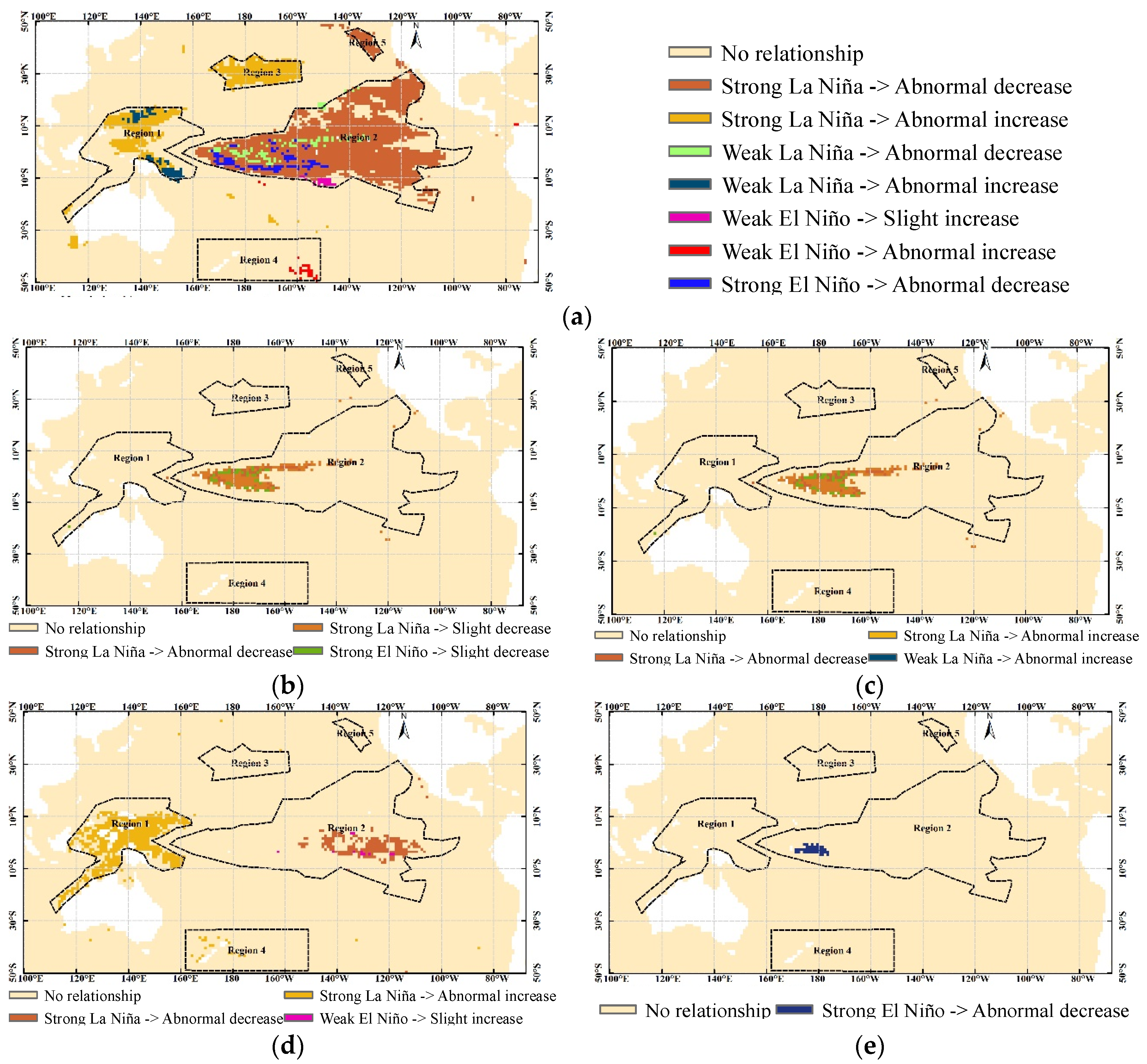
  • The following factors change with La Niña events through oceanic and atmospheric bridge (e.g., the western Pacific warm pool, Kelvin and Rossby wave, trade winds, Walker circulation, equatorial circulation, and the Peru and California Cold Currents): SSTA in the western PO, northern subtropical PO, and offshore of the California coast; SLAA in the southern PO; and WSA in the middle of the equatorial PO.
  • Only abnormal decrease of CHLA in the middle of the equatorial PO is considered a predicator of and response to El Niño events.
  • El Niño events affect variations of SSTA in the middle of the tropical PO and southern PO, SSPA in the middle of the equatorial PO, and SLAA in the east of the equatorial PO. The effects are due to the eastward expansion of displacement of the western Pacific warm pool, variation of trade winds, Kelvin and Rossby wave, Walker circulation and Hadley cell circulation.
  • The association patterns between and among marine environmental parameters and La Niña events are more complicated in mutual relationships and typical in spatial domain than those of El Niño events. The primary reason for this is that the two types of El Niño events dominate different physical processes of the marine environment.

Acknowledgments

We thank the National Oceanic and Atmospheric Administration/The Office of Oceanic and Atmospheric Research/Earth System Research Laboratory/Physical Sciences Division, the Sea-Viewing Wide Field-of-View Sensor and Moderate Resolution Imaging Spectroradiometer projects, the Goddard Distributed Active Archive Center, the Archiving, Validation and Interpretation of Satellites Oceanographic data with support from National Centre for Space Studies, and the Remote Sensing Systems Version-7 Microwave Radiometer Data working group for providing research data. We would also thank the professional English Editing Service, i.e., enago, for providing a spelling and grammar check. This research was supported by the National Natural Science Foundation of China (No. 41371385, No. 41401439 and No. 41671401), the National Key Research and Development Program of China (No. 2016YFA0600304).

Author Contributions

Cunjin Xue led the research work, proposed the idea and structure of this manuscript, wrote the Introduction and Conclusion sections, and integrated the contributions from all authors as a whole. Qing Dong proposed the idea of this manuscript and conceived and designed the experiments, and collaborated with Cunjin Xue to write the Results and Discussion sections. Xing Fan contributed the remote sensing data processing and analyzing algorithm, and collaborated with Cunjin Xue to write the other sections.

Conflicts of Interest

The authors declare no conflict of interest.

References

  1. Chen, G.; Fang, C.Y.; Zhang, C.Y.; Chen, Y. Observing the coupling effect between warm pool and “rain pool” in the Pacific Ocean. Remote Sens. Environ. 2004, 91, 153–159. [Google Scholar] [CrossRef]
  2. Karl, D.M.; Letelier, R.; Hebel, D.; Tupas, L.; Dore, J.; Christian, J.; Winn, C. Ecosystem changes in the North Pacific subtropical gyre attributed to the 1991–1992 El Niño. Nature 1995, 373, 230–234. [Google Scholar] [CrossRef]
  3. Polovina, J.; Howell, J.E.A.; Abecassis, M. Ocean’s least productive waters are expanding. Geophys. Res. Lett. 2008, 35, L03618. [Google Scholar] [CrossRef]
  4. Oliver, M.J.; Irwin, A.J. Objective global ocean biogeographic provinces. Geophys. Res. Let. 2008, 35, L15601. [Google Scholar] [CrossRef]
  5. Milne, G.A.; Gehrels, W.R.; Hughes, C.W.; Tamisiea, M.E. Identifying the causes of sea-level change. Nat. Geosci. 2009, 2, 471–478. [Google Scholar] [CrossRef] [Green Version]
  6. Hollmann, R.; Merchant, C.R.; Saunders, R.; Downy, C.; Buchwitz, M.; Cazenave, A.; Chuvieco, E.; Defourny, P.; DeLeeuw, G.; Forsberg, R.; et al. The ESA climate change initiative: Satellite data records for essential climate variables. Bull. Am. Meteor. Soc. 2013, 94, 1541–1552. [Google Scholar] [CrossRef]
  7. Yang, J.; Gong, P.; Fu, R.; Zhang, M.; Chen, J.; Liang, S.; Xu, B.; Shi, J.; Dickinson, R. The role of satellite remote sensing in climate change studies. Nat. Clim. Chang. 2013, 13, 875–883. [Google Scholar] [CrossRef]
  8. McPhaden, M.J.; Zebiak, S.E.; Glantz, M.H. ENSO as an integrating concept in earth science. Science 2006, 314, 1740–1745. [Google Scholar] [CrossRef] [PubMed]
  9. Camargo, S.J.; Adam, H. Western North Pacific tropical cyclone intensity and ENSO. J. Clim. 2005, 18, 2996–3006. [Google Scholar] [CrossRef]
  10. Wu, B.; Zhou, T.J.; Li, T. Contrast of rainfall-SST relationships in the western North Pacific between the ENSO-developing and ENSO-decaying summers. J. Clim. 2009, 22, 4398–4405. [Google Scholar] [CrossRef]
  11. Picaut, J.; Ioualalen, M.; Menkes, C.; Delcroix, T.; McPhaden, M.J. Mechanism of the zonal displacements of the Pacific warm pool: Implications for ENSO. Science 1996, 274, 1486–1489. [Google Scholar] [CrossRef] [PubMed]
  12. Matsuura, T.; Iizuka, S. Zonal migration of the Pacific warm-pool tongue during El Niño events. J. Phys. Oceanogr. 2000, 30, 1582–1600. [Google Scholar] [CrossRef]
  13. Curtis, S.; Salahuddin, A.; Adler, R.F.; Huffman, G.J.; Gu, G.; Hong, Y. Precipitation extremes estimated by GPCP and TRMM: ENSO relationships. J. Hydrometeor. 2007, 8, 678–689. [Google Scholar] [CrossRef]
  14. Murtugudde, R.; Wang, L.P.; Hackert, E.; Beauchamp, J.; Christian, J.; Busalacchi, A. Remote sensing of the Indo-Pacific region: Ocean colour, sea level, winds and sea surface temperatures. Int. J. Remote Sens. 2004, 25, 1423–1435. [Google Scholar] [CrossRef]
  15. Mennis, J.; Liu, J.W. Mining association rules in spatio-temporal data: An analysis of urban socioeconomic and land cover change. Trans. GIS 2005, 9, 13–18. [Google Scholar] [CrossRef]
  16. Korting, T.S.; Fonseca, L.M.G.; Camara, G. GeoDMA—Geographic data mining analyst. Comput. Geosci.-UK 2013, 57, 133–145. [Google Scholar] [CrossRef]
  17. Levy, G.; Gower, J. Oceanic manifestation of global changes: Satellite observations of the atmosphere, ocean and their interface. Int. J. Remote Sens. 2010, 31, 4509–4514. [Google Scholar] [CrossRef]
  18. Kahru, M.; Gille, S.T.; Murtugudde, R.; Strutton, P.G.; Manzano-Sarabia, M.; Wang, H.; Mitchell, B.G. Global correlations between winds and ocean chlorophyll. J. Geophys. Res. Ocean. 2010, C12040, 115. [Google Scholar]
  19. Radenac, M.H.; Léger, F.; Singh, A.; Delcroix, T. Sea surface chlorophyll signature in the tropical Pacific during eastern and central Pacific ENSO events. J. Geophys. Res. Ocean. 2012, 117, C04007. [Google Scholar] [CrossRef]
  20. Wilson, C.; Adamec, D. Correlations between surface chlorophyll and sea surface height in the tropical Pacific during the 1997–1999 El Niño-Southern Oscillation event. J. Geophys. Res. Ocean. 2001, 106, 31175–31188. [Google Scholar] [CrossRef]
  21. Park, J.Y.; Kug, J.S.; Park, Y.J. An exploratory modeling study on bio-physical processes associated with ENSO. Prog. Oceanogr. 2014, 124, 28–41. [Google Scholar] [CrossRef]
  22. Park, J.Y.; Kug, J.S.; Park, Y.J.; Yeh, S.W.; Jang, C.J. Variability of chlorophyll associated with El Niño-Southern Oscillation and its possible biological feedback in the equatorial Pacific. J. Geophys. Res. Ocean. 2011, 116. [Google Scholar] [CrossRef]
  23. Casey, K.S.; Adamec, D. Sea surface temperature and sea surface height variability in the North Pacific Ocean from 1993 to 1999. J. Geophy. Res.-Ocean. 2002, 107, 3099. [Google Scholar] [CrossRef]
  24. Wang, C.; Fiedler, P.C. ENSO variability and the eastern tropical Pacific: A review. Prog. Oceanogr. 2006, 69, 239–266. [Google Scholar] [CrossRef]
  25. Yokoyama, C.; Takayabu, Y.N. Relationships between rain characteristics and environment. Part I: TRMM precipitation features and the large-scale environment over the tropical Pacific. Mon. Weather Rev. 2012, 140, 2831–2840. [Google Scholar] [CrossRef]
  26. Xue, C.J.; Song, W.J.; Qin, L.J.; Dong, Q.; Wen, X.Y. A spatiotemporal mining framework for abnormal association patterns in marine environments with a time series of remote sensing images. Int. J. Appl. Earth Obs. 2015, 38, 105–114. [Google Scholar] [CrossRef]
  27. Xue, C.J.; Dong, Q.; Fan, X. Spatiotemporal association patterns of multiple parameters in the northwestern Pacific Ocean and their relationships with ENSO. Int. J. Remote Sens. 2014, 35, 4467–4483. [Google Scholar] [CrossRef]
  28. Ganguly, A.; Steinhaeuser, K. Data Mining for Climate Change and Impacts. In Proceedings of the IEEE International Conference on Data Mining Workshops, ICDMW, Pisa, Italy, 15–19 Decmber 2008; pp. 385–394.
  29. Saulquin, B.; Fablet, R.; Mercier, G.; Demarcq, H.; Mangin, A.; Fantond’Andon, O.H. Multiscale Event-Based Mining in Geophysical Time Series: Characterization and Distribution of Significant Time-Scales in the Sea Surface Temperature Anomalies Relatively to ENSO Periods from 1985 to 2009. IEEE J. Sel. Top. Appl. Earth Obs. Remote Sens. 2014, 7, 3543–3552. [Google Scholar] [CrossRef]
  30. Kumar, V. Discovery of patterns in global earth science data using data mining. Lect. Notes Comput. Sci. 2010, 6118. [Google Scholar] [CrossRef]
  31. Holloway, P.; Miller, J.A. Exploring spatial scale, autocorrelation and nonstationarity of bird species richness patterns. ISPRS Int. J. Geo-Inf. 2015, 4, 783–798. [Google Scholar] [CrossRef]
  32. Wang, H.; Zhang, J.F.; Zhu, F.B.; Zhang, W.W. Analysis of spatial pattern of aerosol optical depth and affecting factors using spatial autocorrelation and spatial autoregressive model. Environ. Earth Sci. 2016, 75, 822. [Google Scholar]
  33. Su, F.Z.; Zhou, C.H.; Lyne, V.; Du, Y.Y.; Shi, W.Z. A data mining approach to determine the spatio-temporal relationship between environmental factors and fish distribution. Ecol. Model. 2004, 174, 421–431. [Google Scholar] [CrossRef]
  34. Huang, P.Y.; Kao, L.J.; Sandnes, F.E. Efficient mining of salinity and temperature association rules from ARGO data. Expert Syst. Appl. 2008, 35, 59–68. [Google Scholar] [CrossRef]
  35. Reynolds, R.W.; Rayner, N.A.; Smith, T.M.; Stokes, D.C.; Wang, W. An improved in situ and satellite SST analysis for climate. J. Clim. 2002, 15, 1609–1625. [Google Scholar] [CrossRef]
  36. Hooker, S.B.; McClain, C.R. The calibration and validation of SeaWiFS data. Prog. Oceanogr. 2000, 45, 427–465. [Google Scholar] [CrossRef]
  37. MSLA—Monthly Mean and Climatology Maps of Sea Level Anomalies. Available online: http://www.aviso.altimetry.fr/en/data/products/sea-surface-height-products/global/msla-mean-climatology.html (accessed on 20 January 2017).
  38. Remote Sensing Systems (RSS). Available online: http://data.remss.com/ccmp/v02.0/ (accessed on 20 January 2017).
  39. Wolter, K.; Timlin, M.S. El Nino/Southern Oscillation behaviour since 1871 as diagnosed in an extended multivariate ENSO index (MEI. ext). Int. J. Climatol. 2011, 31, 1074–1087. [Google Scholar] [CrossRef]
  40. Xue, C.J.; Song, W.J.; Qin, L.J.; Dong, Q. A normalized-mutual-information-based mining method for marine abnormal association rules. Comput. Geosci.-UK 2015, 76, 121–129. [Google Scholar]
  41. Srikant, R.; Agrawal, R. Mining sequential patterns: Generalizations and performance improvements. In Proceedings of the 5th International Conference on Extending Database Technology (EDBT’96), Avignon, France, 25–29 March 1996; pp. 3–17.
  42. Li, X.Y.; Zhai, P.M. On indices and indictors of ENSO episodes. Acta Metall. Sin. 2000, 58, 102–119. [Google Scholar]
  43. Trenberth, K.E. The definition of El Niño. Bull. Am. Meteor. Soc. 1997, 78, 2771–2777. [Google Scholar] [CrossRef]
  44. Messié, M.; Chavez, F.P. A global analysis of ENSO synchrony: The oceans’ biological response to physical forcing. J. Geophys. Res. Ocean. 2012, 117, C09001. [Google Scholar] [CrossRef]
  45. Curtis, S.; Adler, R. ENSO indices based on patterns of satellite-derived precipitation. J. Clim. 2000, 13, 786–2793. [Google Scholar] [CrossRef]
  46. Yu, J.Y.; Liu, W.T.; Mechos, C.R. An SST anomaly dipole in the northern subtropical pacific and its relationships with ENSO. Geophys. Res. Lett. 2000, 27, 1931–1934. [Google Scholar] [CrossRef]
  47. Messié, M.; Chavez, F.P. Physical-biological synchrony in the global ocean associated with recent variability in the central and western equatorial Pacific. J. Geophys. Res. Ocean. 2013, 118, 3782–3794. [Google Scholar] [CrossRef]
  48. Li, Z.X. Influence of Tropical Pacific El Nino on the SST of the Southern Ocean through atmospheric bridge. Geophys. Res. Lett. 2000, 27, 3505–3508. [Google Scholar] [CrossRef]
  49. Ashok, K.; Behera, S.K.; Rao, S.A.; Weng, H.; Yamagata, T. El Niño Modoki and its possible teleconnection. J. Geophys. Res. Ocean. 2007, C11007. [Google Scholar] [CrossRef]
  50. Larkin, N.K.; Harrison, D.E. Global seasonal temperature and precipitation anomalies during El Niño autumn and winter. Geophys. Res. Lett. 2005, 32, L16705. [Google Scholar] [CrossRef]
  51. Ashok, K.; Yamagata, T. The El Niño with a difference. Nature 2009, 461, 481–484. [Google Scholar] [CrossRef] [PubMed]
Figure 1. A flowchart of this manuscript.
Ijgi 06 00032 g001
Figure 2. Five more interactive regions among marine environments and ENSO in the Pacific Ocean (PO).
Ijgi 06 00032 g002
Figure 3. Variations in marine environment causing ENSO events in PO. (a) Association pattern from SSTA to ENSO; (b) Association pattern from SSPA to ENSO; (c) Association pattern from SLAA to ENSO; (d) Association pattern from WSA to ENSO; (e) Association pattern from CHLA to ENSO.
Ijgi 06 00032 g003
Figure 4. Variations in marine environment caused by ENSO events in PO. (a) Association pattern from ENSO to SSTA; (b) Association pattern from ENSO to SSPA; (c) Association pattern from ENSO to WSA; (d) Association pattern from ENSO to SLAA; (e) Association pattern from ENSO to CHLA.
Ijgi 06 00032 g004
Figure 5. Association patterns network for La Niña events and marine environmental parameters. The mutual relationship between X and Y ( X Y ) means that X has enough information to tell Y occurrences, and meanwhile, Y has enough information to tell X occurrences, which are shaded in gray boxes. The one-way relationship from X to Y (XY) means that X has enough information to tell Y occurrences.
Ijgi 06 00032 g005
Figure 6. Association patterns network for El Niño events and marine environmental parameters. The mutual relationship and one-way relationship have the same meanings as Figure 5.
Ijgi 06 00032 g006
Table 1. Sources and resolutions of remote sensing products and multivariate ENSO index (MEI) used in this manuscript.
NoProductSourceTimespanTemporal ResolutionSpatial CoverageSpatial Resolution
1SST 1NOAA/PSDDecember 1981–April 2014MonthlyGlobal1° × 1°
2CHL 2SeaWifsSeptember 1997–November 2010MonthlyGlobal9 km × 9 km
MODISJuly 2002–May 2014MonthlyGlobal9 km × 9 km
3SSP 3TRMMJanuary 1998–February 2014MonthlyGlobal0.25° × 0.25°
4SLA 4AVISOJanuary 1993–December 2012MonthlyGlobal0.25° × 0.25°
5WindSpeed 5RSSJanuary 1988–December 2012MonthlyGlobal0.25° × 0.25°
6ENSO 6MEIJanuary 1950–May 2014Monthly--
1 Provided by National Oceanic and Atmospheric Administration (NOAA)/The Office of Oceanic and Atmospheric Research (OAR)/Earth System Research Laboratory (ESRL) Physical Sciences Division (PSD) [35]; 2 Obtained from the Sea-Viewing Wide Field-of-View Sensor (SeaWiFS) and Moderate Resolution Imaging Spectroradiometer (MODIS) projects and their level-three standard mapped images (SMI) [36]; 3 Obtained from Version 7 of the Tropical Rainfall Measuring Mission (TRMM Product 3B43) provided by the Goddard Distributed Active Archive Center (GES DISC DAAC); 4 Produced by Ssalto/Duacs and distributed by Archiving, Validation and Interpretation of Satellites Oceanographic data (AVISO) with support from National Centre for Space Studies [37]; 5 Obtained from Remote Sensing Systems (RSS) Version-7 Microwave Radiometer Data, available at [38]; 6 Provided by NOAA-ESRL Physical Sciences Division [39].
Table 2. El Niño and La Niña events’ characterizations during the period of January 1998 to December 2012.
El Niño EventsLa Niña Events
CharacterizationsStart Time–End Time CharacterizationsStart Time–End Time
1Strong January 1998–June 19981StrongSeptember 1998–March 2000
2StrongMay 2002–March 20032Weak November 2000–March 2001
3WeakAugust 2004–May 20053WeakDecember 2005–April 2006
4Strong June 2006–February 20074StrongAugust 2007–April 2008
5Strong June 2009–May 20105WeakSeptember 2008–March 2009
6StrongMay 2012–August 20126StrongJuly 2010–April 2011
7Strong September 2011–February 2012

