Inverse Parametrization of a Regional Groundwater Flow Model with the Aid of Modelling and GIS: Test and Application of Different Approaches

 , , , and
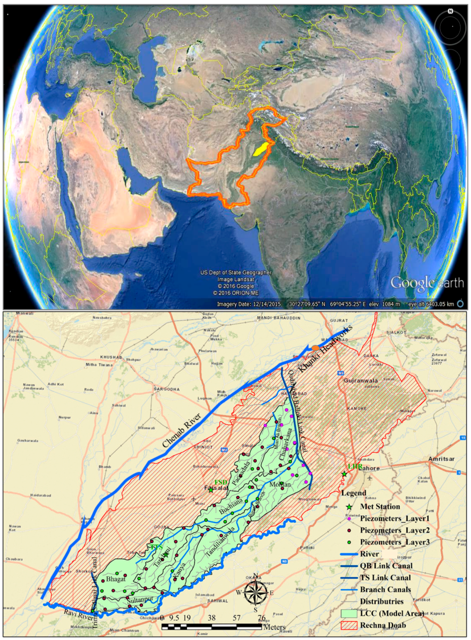
Abstract
:1. Introduction
2. Description of the Study Area
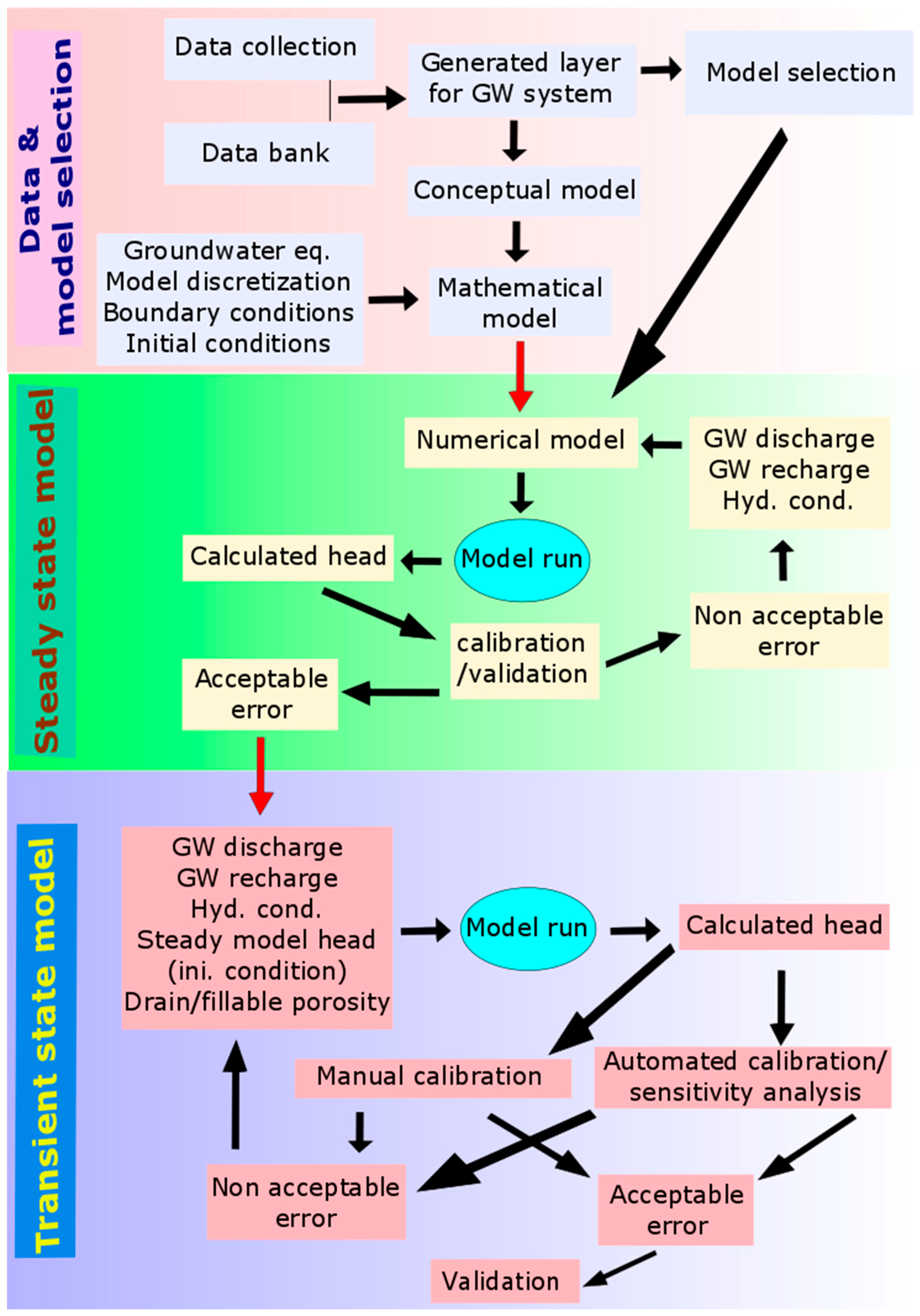
3. Development of Conceptual Model
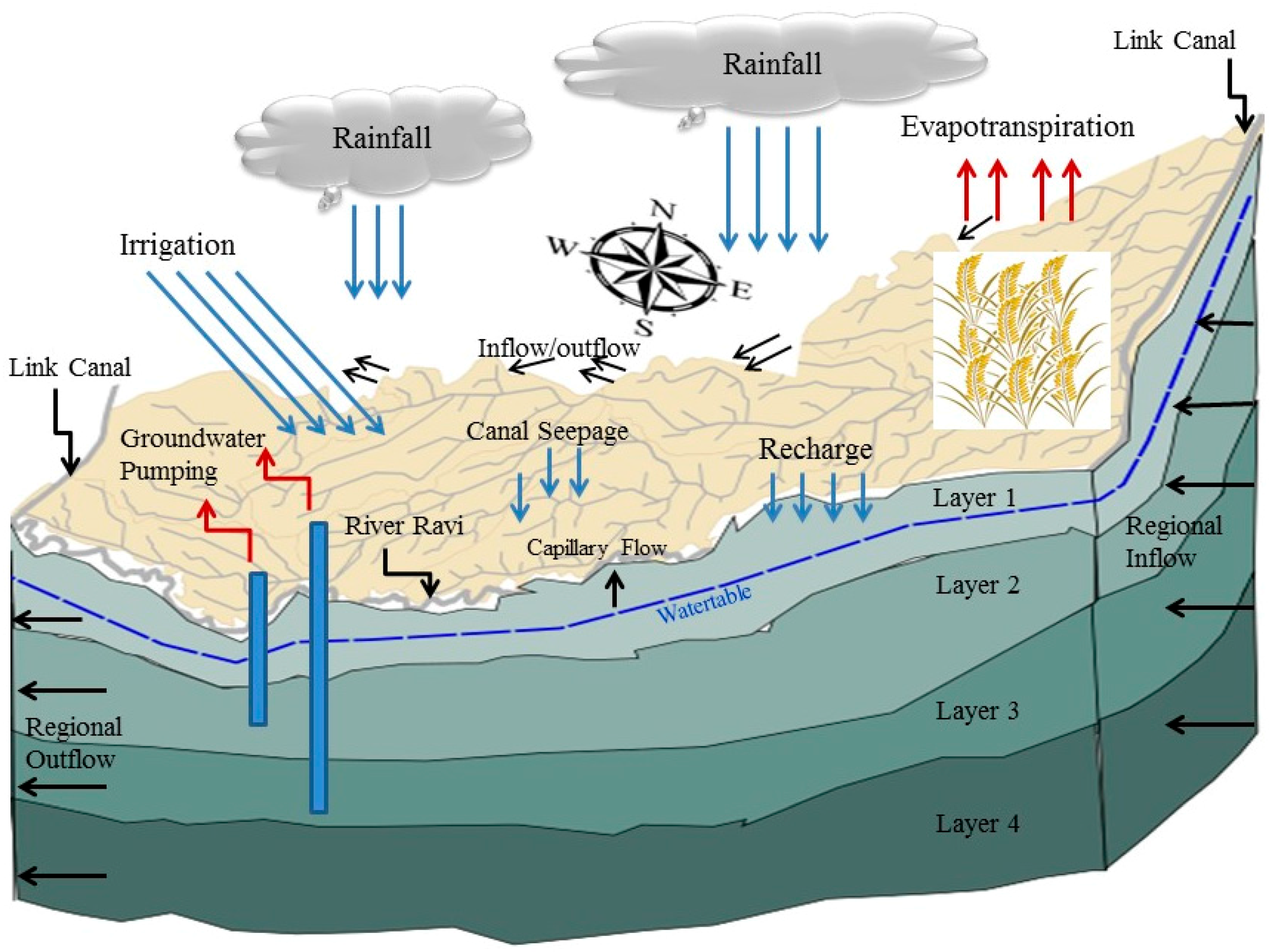
3.1. Processes
3.2. Hydraulic Properties and Geological Scheme
3.3. Data Collection
3.3.1. Maps, Shape Files of Natural Features
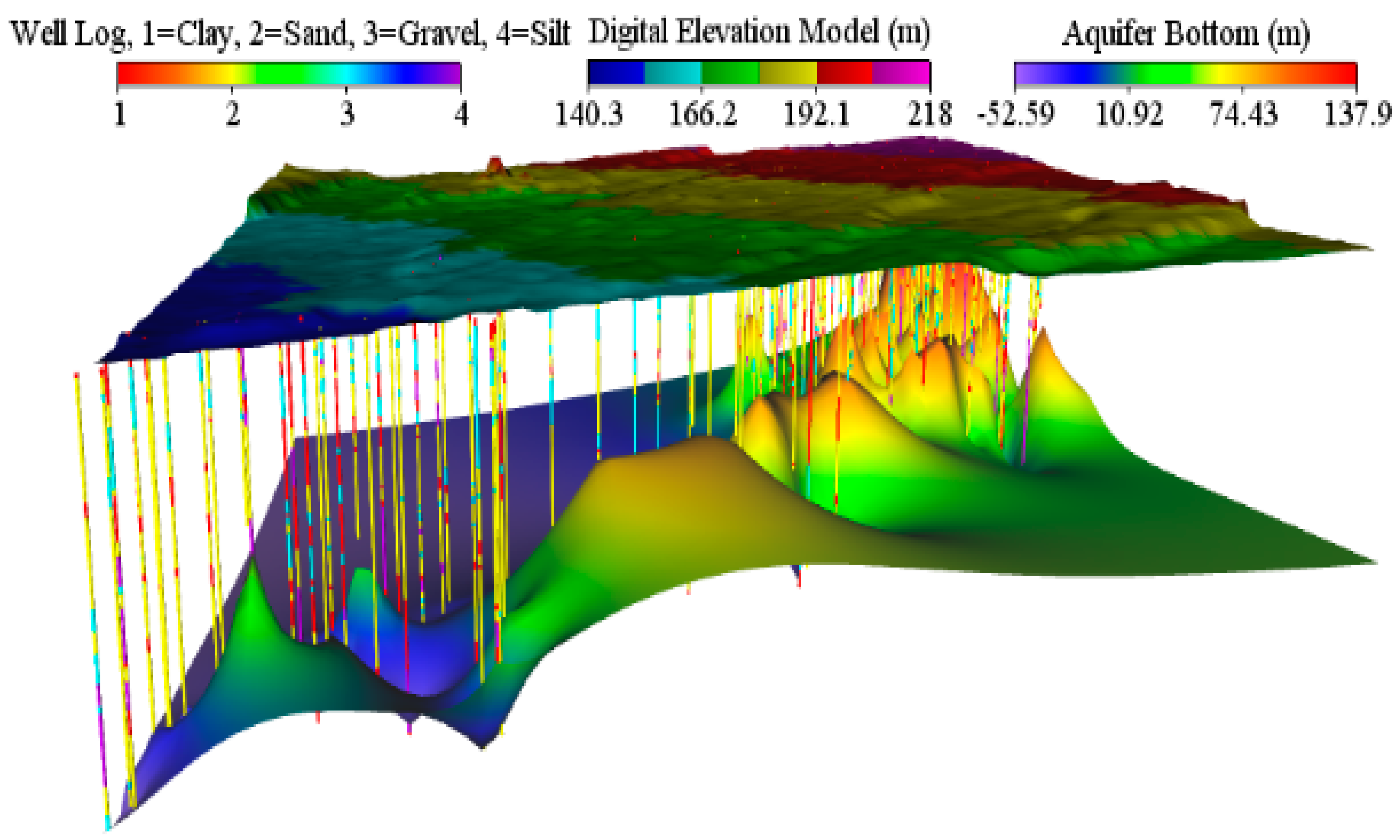
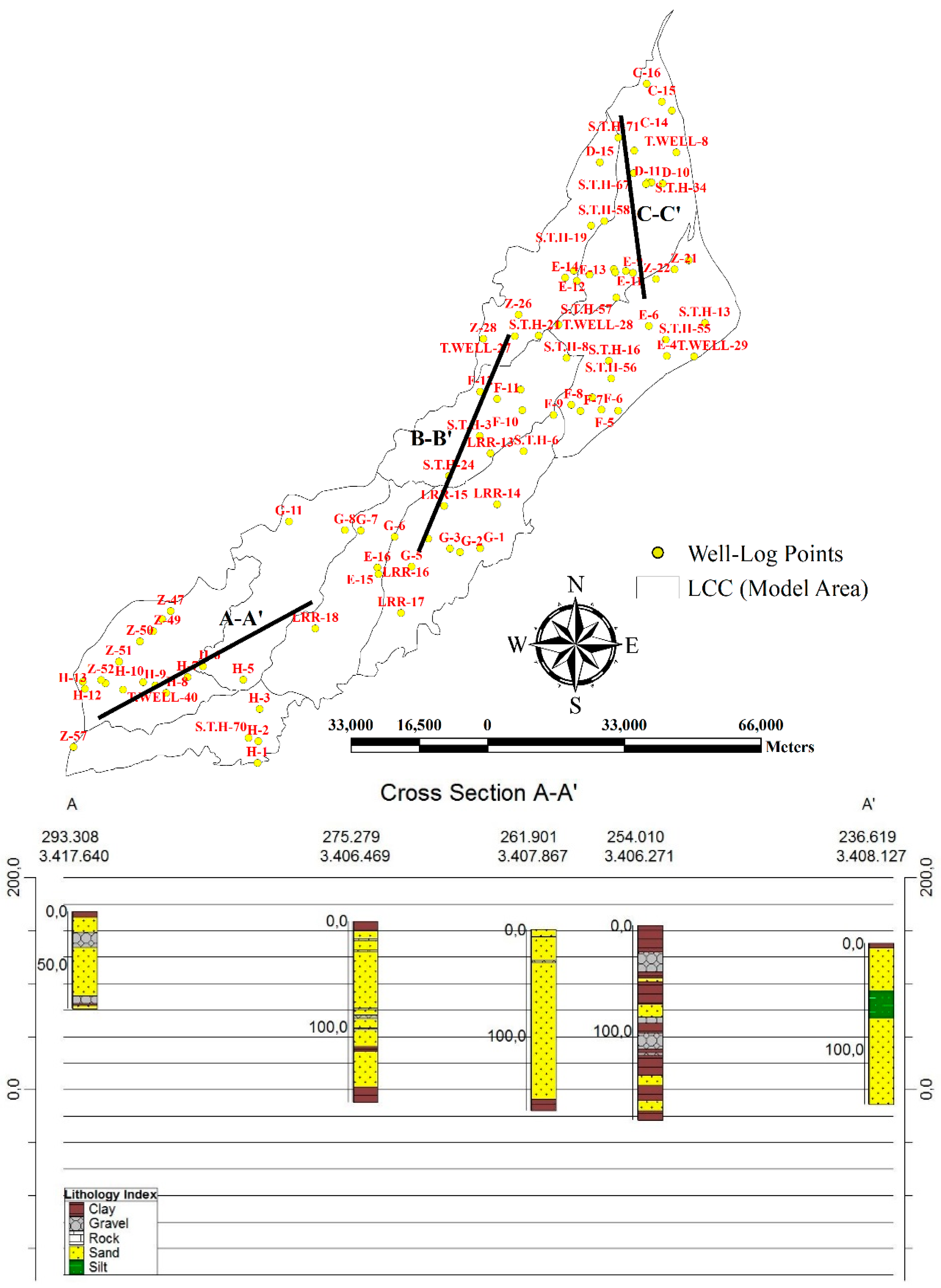
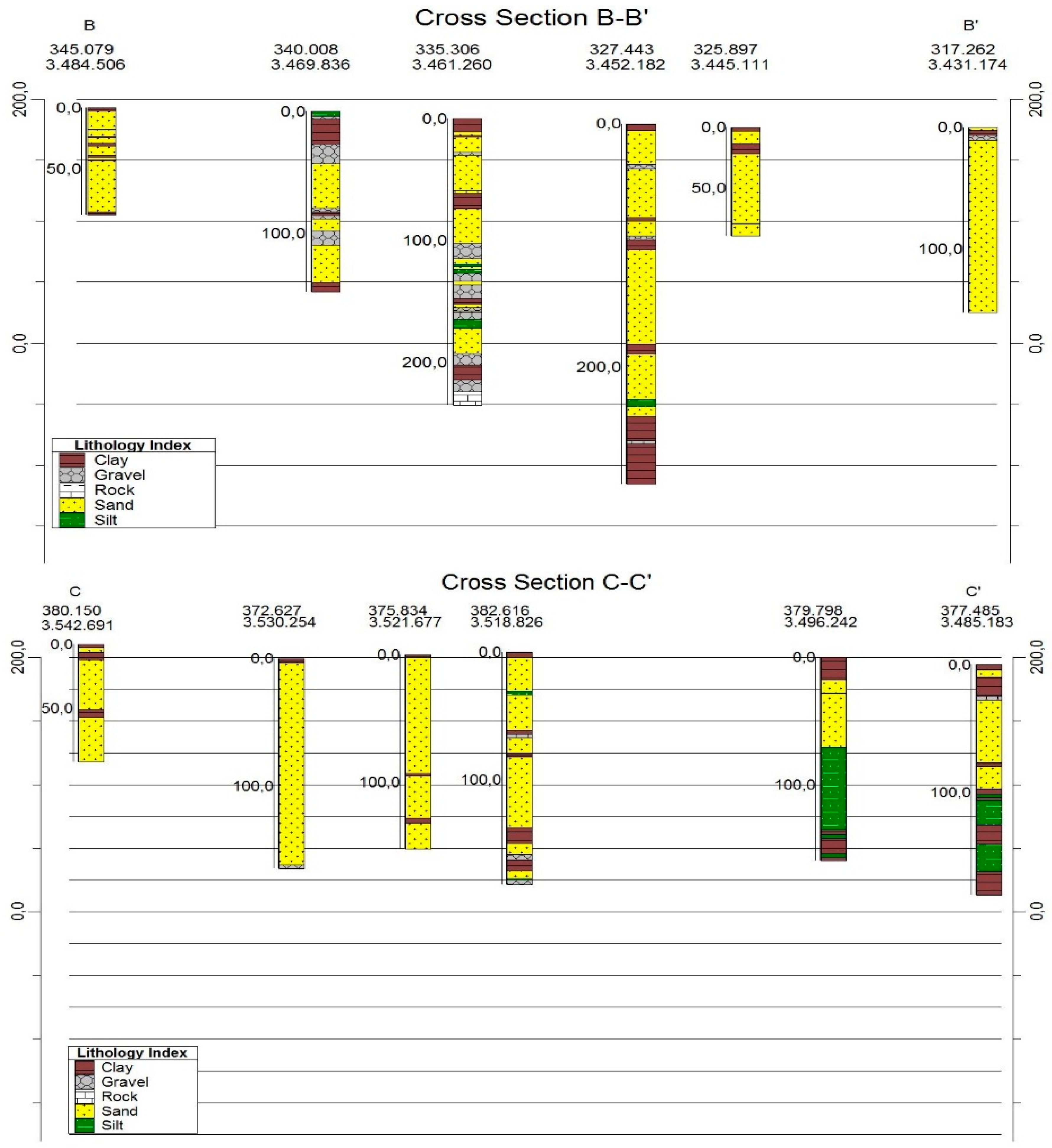
3.3.2. Elevation and Well Log Data
3.3.3. Material Properties and Model Parameters
4. Development of Mathematical Model
4.1. Theory of Groundwater Flow
4.2. Setup of Numerical Model Using FEFLOW
4.2.1. Mesh Generation and Setting of Modelling Problem
4.2.2. Regionalization of Hydraulic Properties
4.2.3. Setting up Different Model Boundary Conditions
4.3. Model Calibration and Parameter Estimation
4.3.1. Functionality of PEST for Model Calibration and Parameters Sensitivities
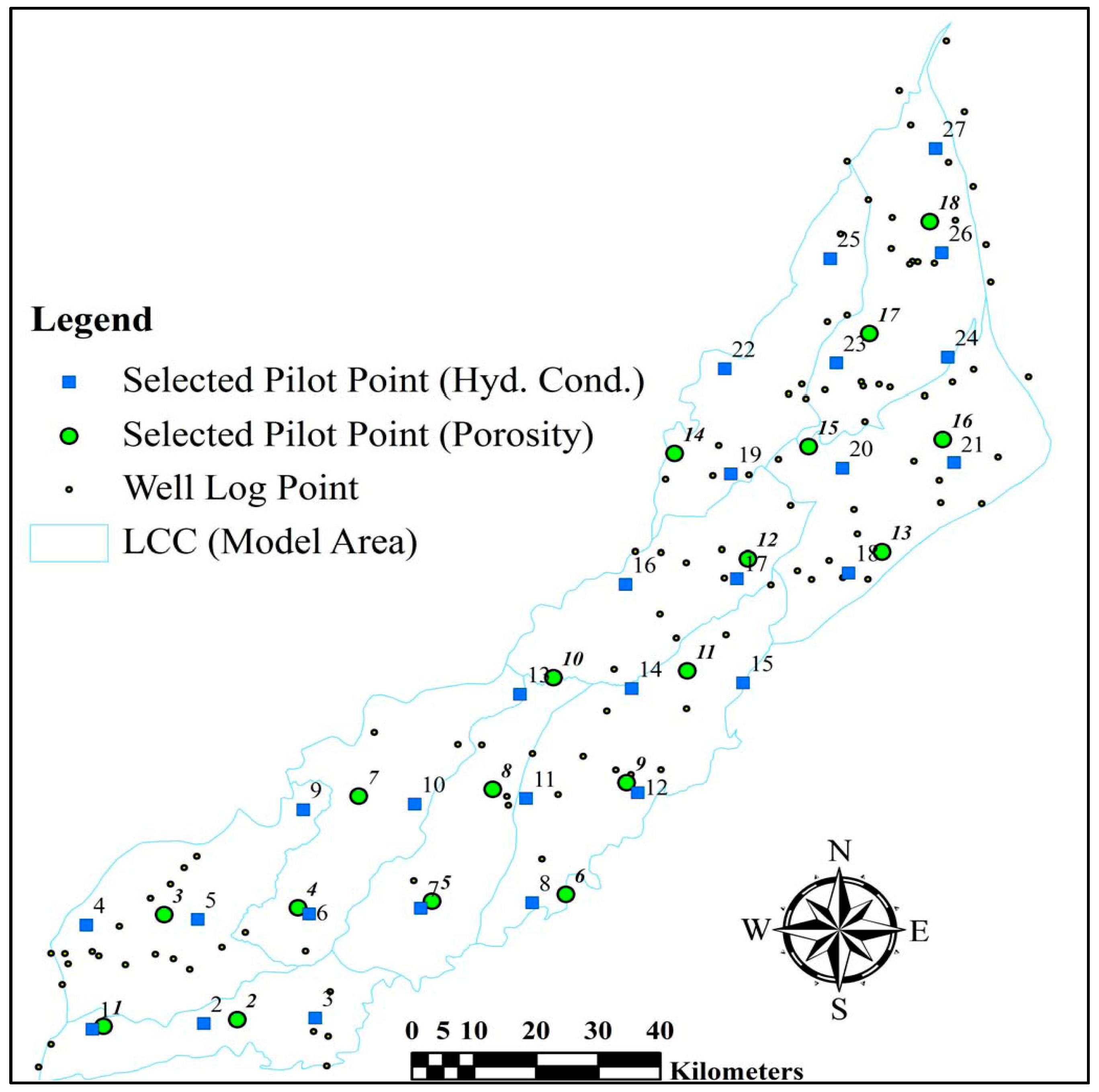
4.3.2. Pilot Point Calibration Technique
4.3.3. Tikhonov Regularization
4.4. Statistical Analysis
5. Results and Discussion
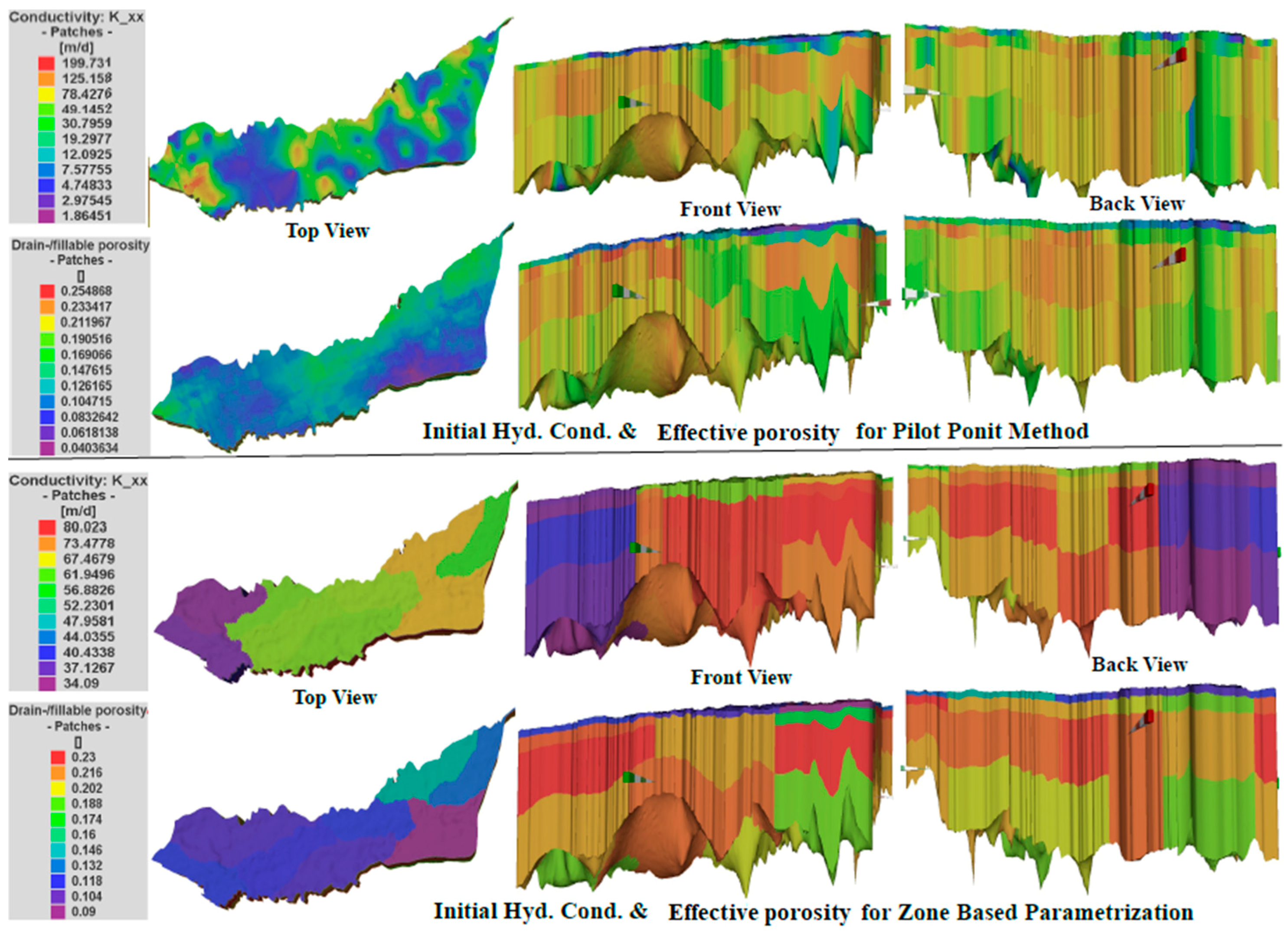
5.1. Selection of Calibration Parameters and Their Initial Values
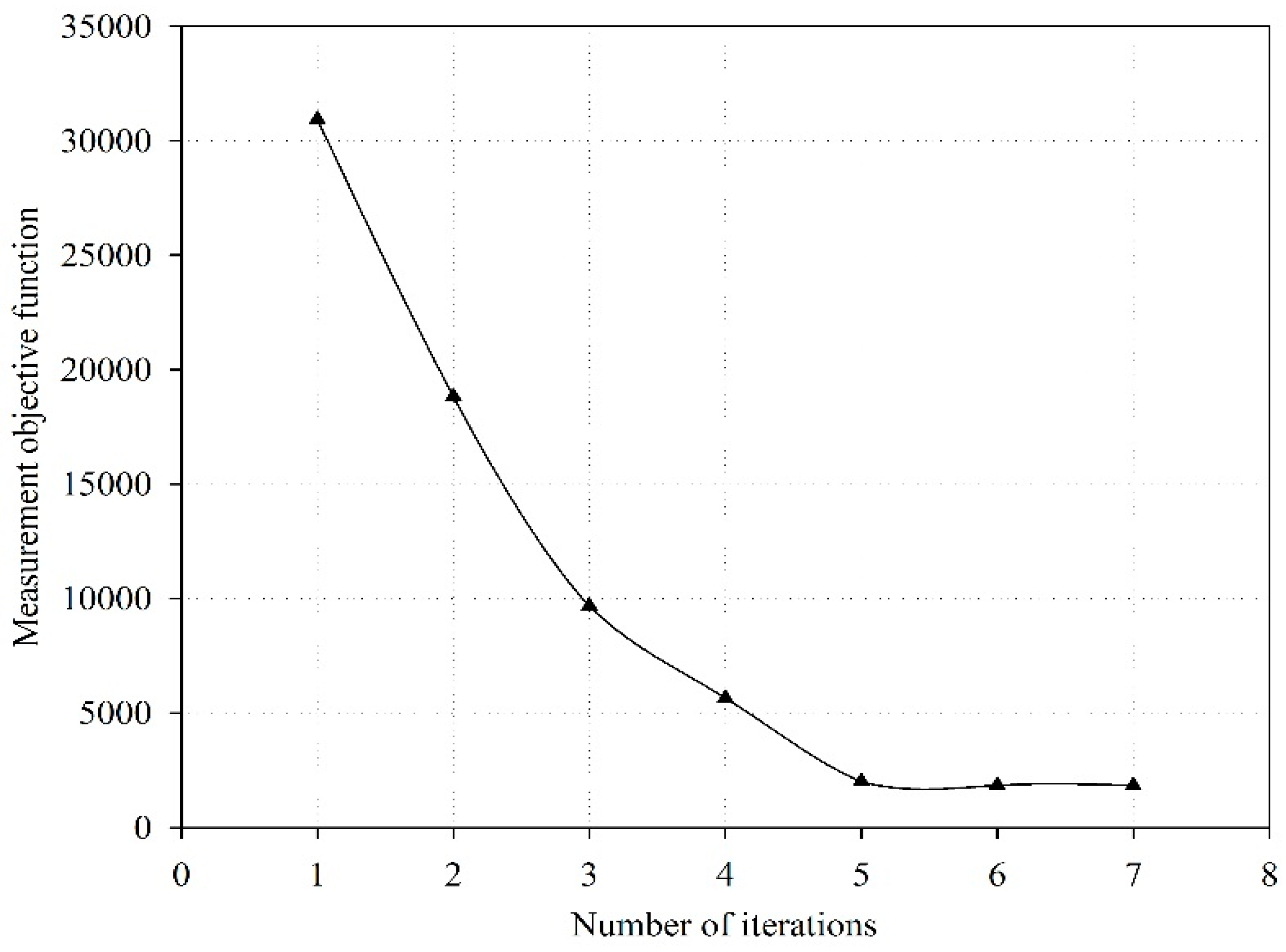
5.2. Calibration and Validation Results for Transient Model under Pilot Points
5.3. Comparison of Calibration Results from Different Methods
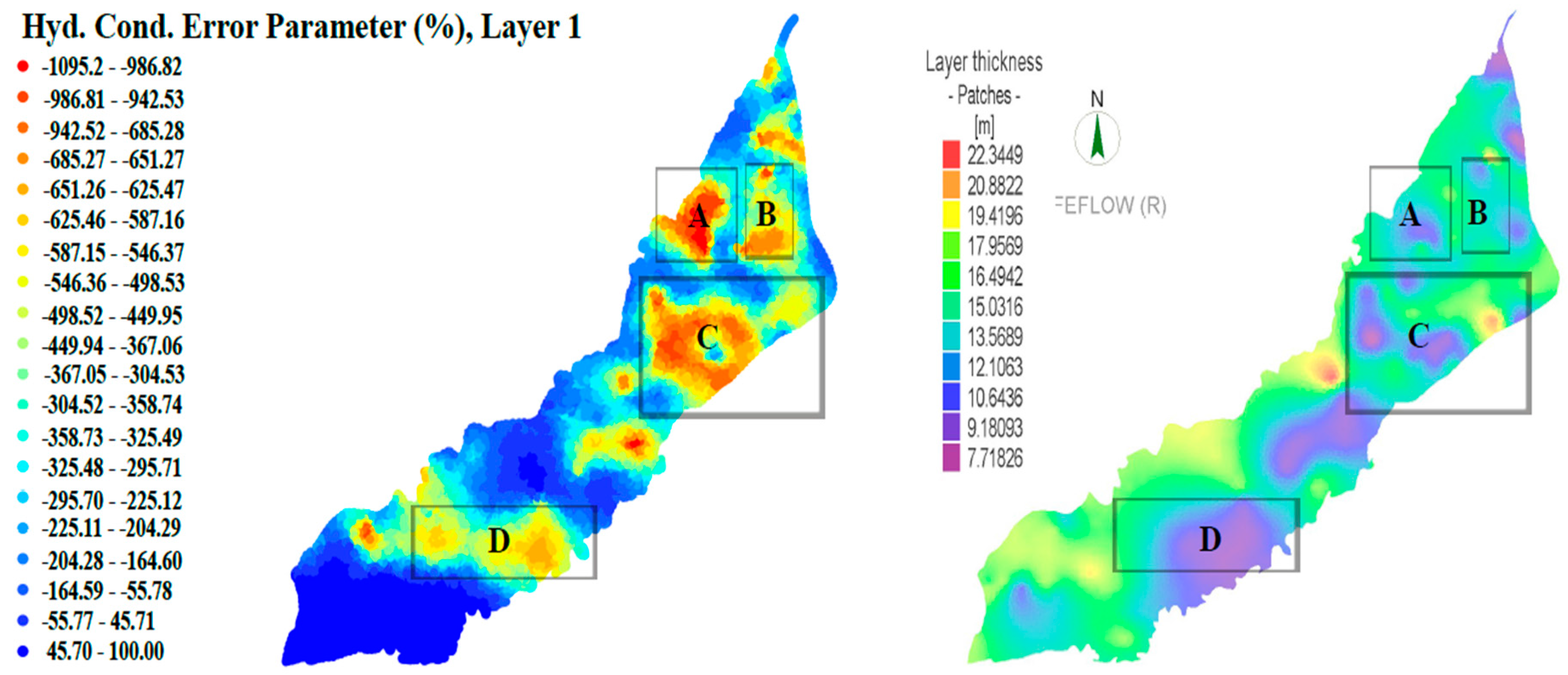
5.4. Model Parameter Sensitivities and Parameter Error
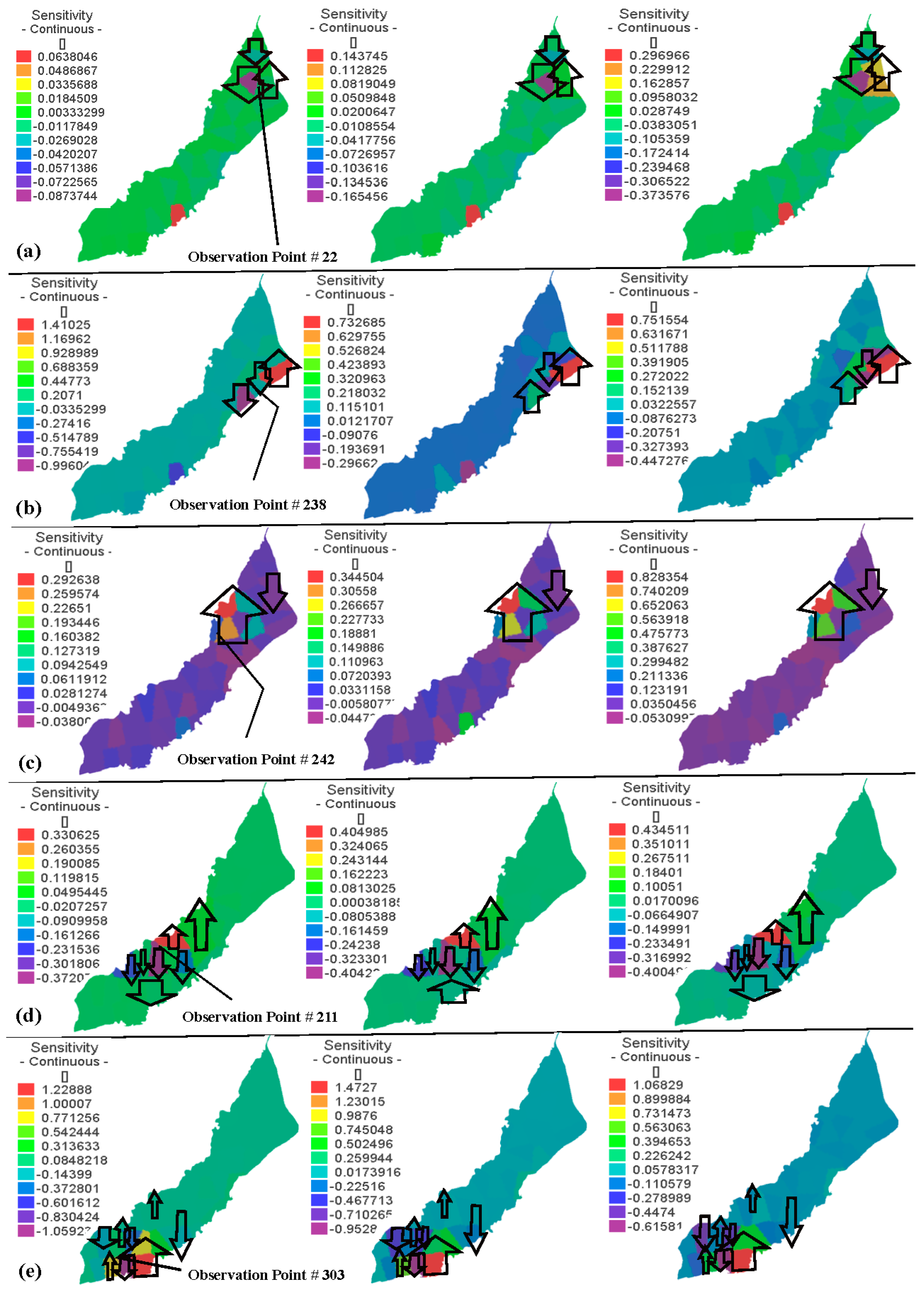
5.5. Sensitivities at Selected Observation Points
6. Conclusions and Outlook
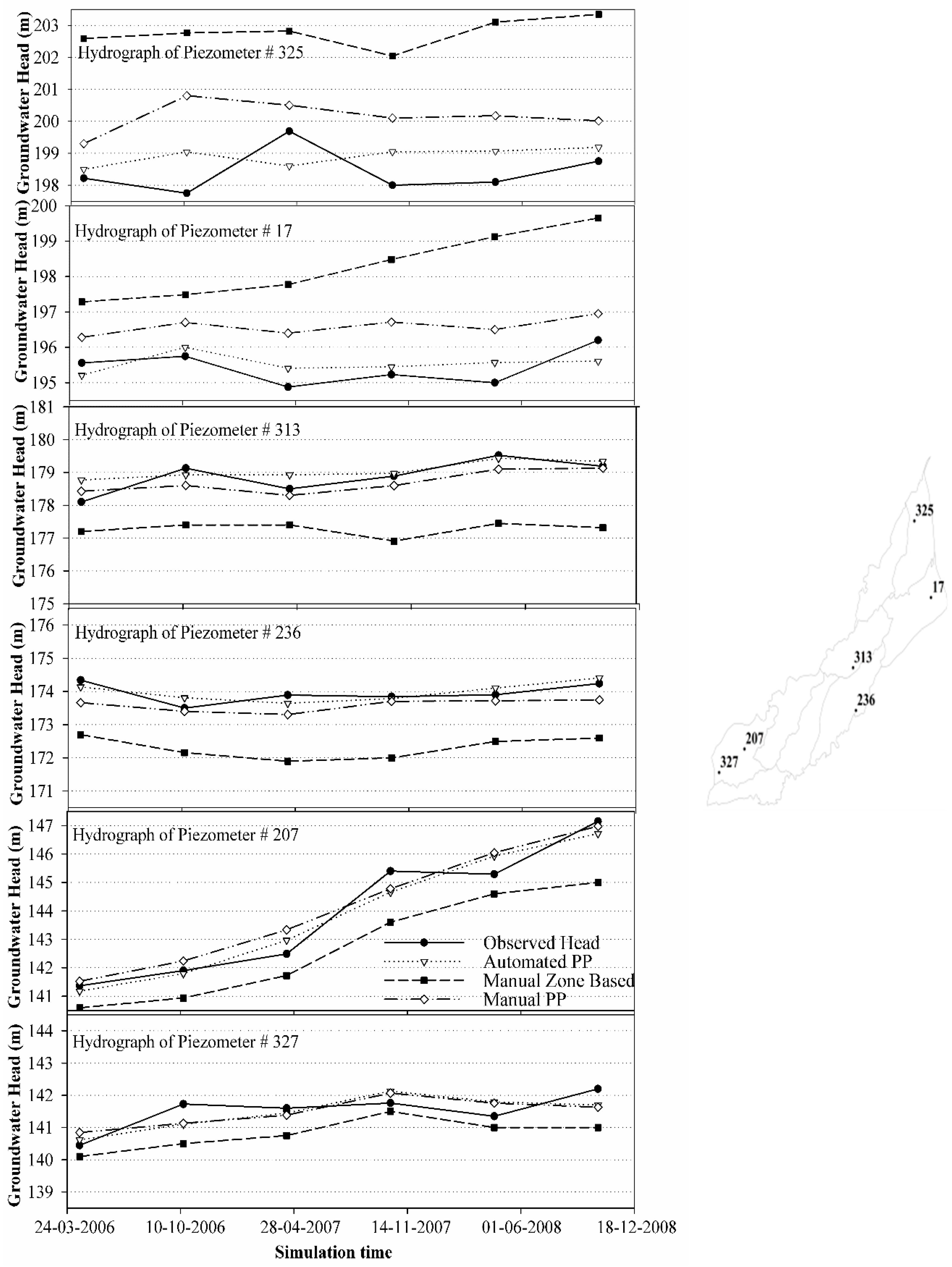
- It is found that the automated pilot point calibration method is more flexible and robust in comparison to manual approaches using pilot point and zone-based parameterization of the model due to its lesser subjectivity on part of the modeller’s experience.
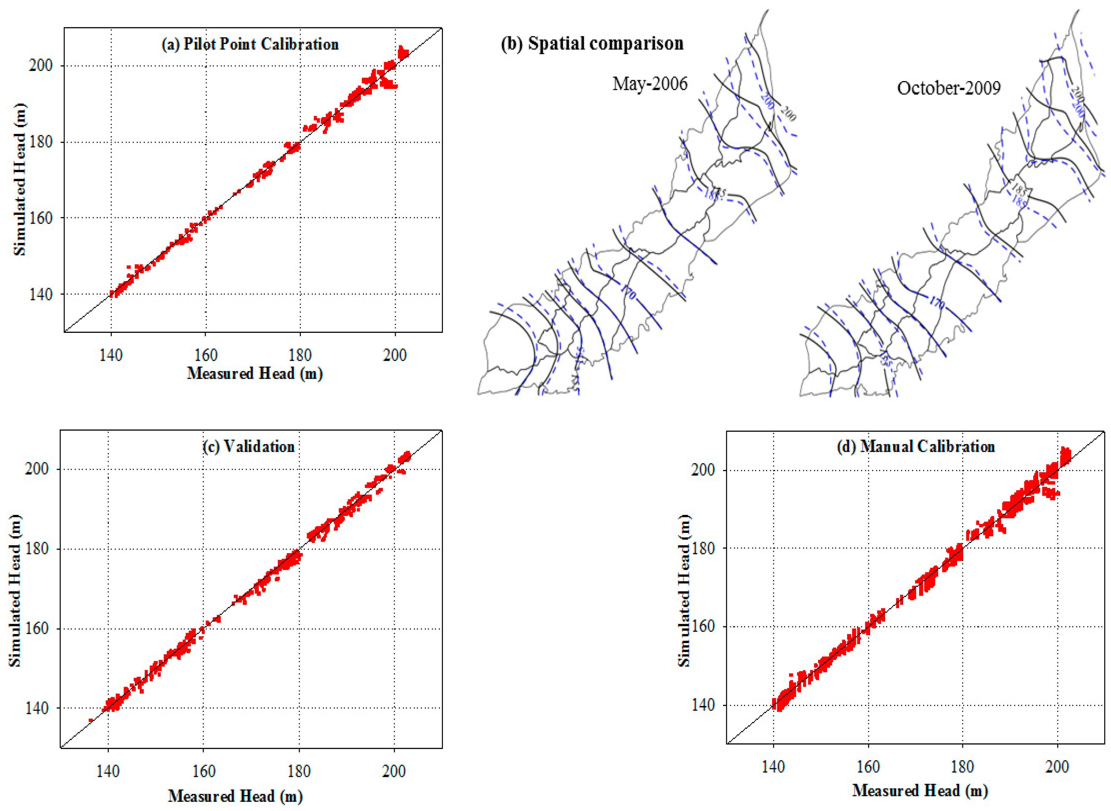
- Automated pilot point calibration results in a reliable model calibration and validation for a majority of model regions as different statistical indicators show reasonable values. For calibration of the transient case, the values of R2, Nash Sutcliffe Efficiency, % BIAS and RMSE are 0.99, 0.976, 0.026 and 1.23 m, respectively, and for validation, the values are 0.987, 0.969, −0.205 and 1.31 m, respectively.
- Apart from the lower calibration efficiency, it is also observed that manual calibration is tedious and cumbersome due to more model runs to get reasonable results.
- The spatial comparison of model calibrations shows that the pilot point approach yields overall better results at different locations with some higher differences at upper locations as compared to zone-based model calibration.
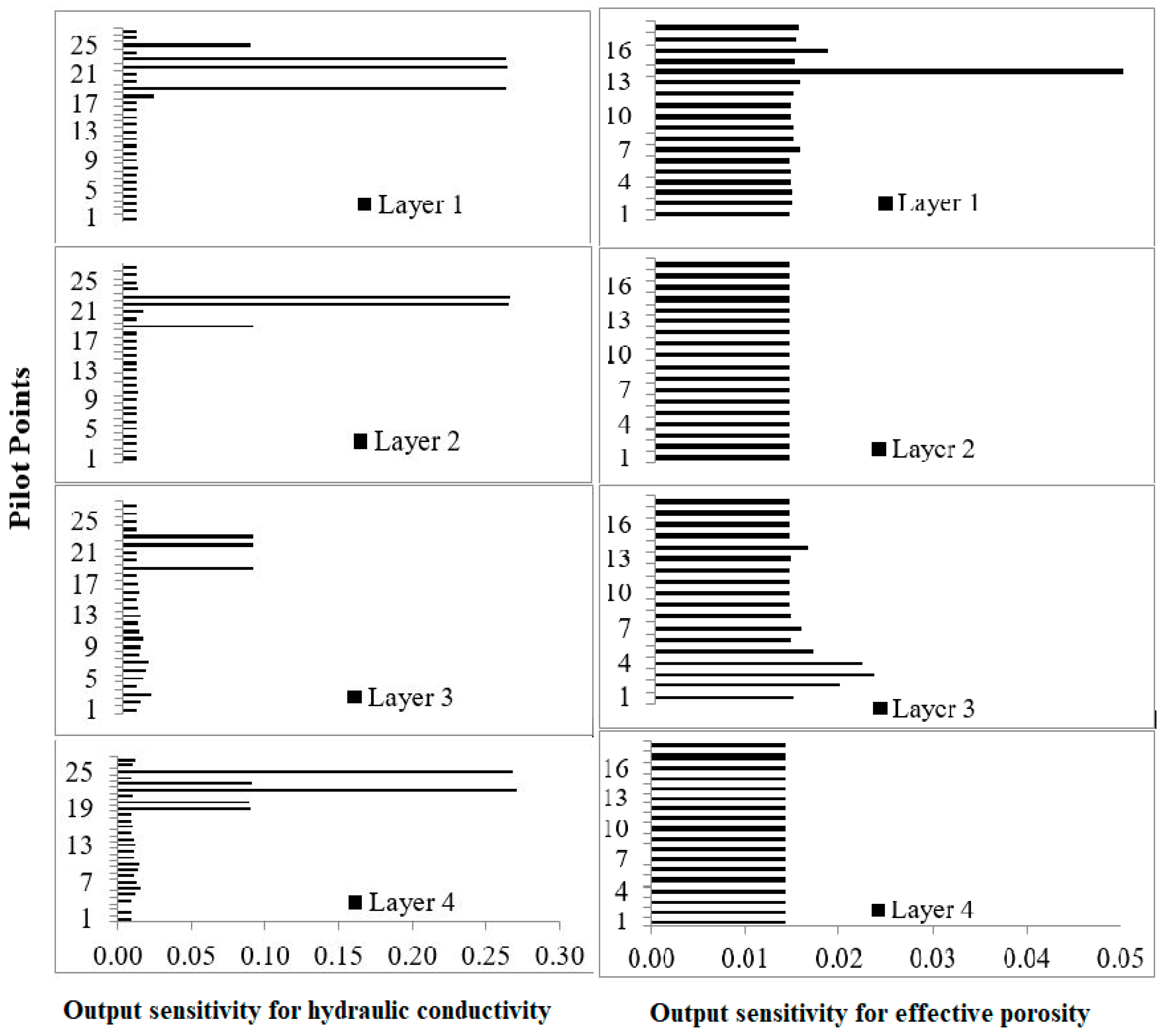
- Parameter sensitivity analysis shows that overall hydraulic conductivity is more influential as compared to effective porosity. However, this sensitivity is quite variable for different model locations and model layers.
- Sensitivities and error parameter results also address limitations/deficiencies of current hydraulic field data and help to identify regions where further field investigations could be planned.
- Sensitivities of different observation points demark different regions of particular importance and therefore guide planners to perform field activities there in future.
- Present sensitivity analysis was performed by a local approach employed in PEST. For such methods, there is always a possibility that the entire parameter space might not be well represented which could be addressed in future by some global sensitivity analysis approach.
- Predictive analysis is another way to explore uncertainties of model results. For the current study, it was attempted; however, the use of such analysis is only limited to a well-posed problem which was not the case for the current model. If a problem is ill-posed, then it does not work because pertinent matrices become un-invertible. The only possibility then left is to explore non-linear uncertainty analysis options. PEST has provided utilities like PREDUNC and/or GENLINPRED for this purpose. Null space Monte Carlo and running model in “Pareto” mode could be alternative solutions. Hence, it is recommended to explore these different approaches in future studies.
Supplementary Materials
Acknowledgments
Author Contributions
Conflicts of Interest
References
- Kazmi, S.I.; Ertsen, M.W.; Asi, M.R. The impact of conjunctive use of canal and tube well water in Lagar irrigated area, Pakistan. Phys. Chem. Earth Parts A/B/C 2012, 47–48, 86–98. [Google Scholar] [CrossRef]
- Shah, T.; Debroy, A.; Qureshi, A.S.; Wang, J. Sustaining Asia’s groundwater boom: An overview of issues and evidence. Nat. Resour. Forum 2003, 27, 130–141. [Google Scholar] [CrossRef]
- Qureshi, A.S.; Gill, M.A.; Sarwar, A. Sustainable groundwater management in Pakistan: Challenges and opportunities. Irrig. Drain. 2010, 59, 107–116. [Google Scholar] [CrossRef]
- Sarwar, A.; Eggers, H. Development of a conjunctive use model to evaluate alternative management options for surface and groundwater resources. Hydrogeol. J. 2006, 14, 1676–1687. [Google Scholar] [CrossRef]
- Qureshi, A.S.; McCornick, P.G.; Sarwar, A.; Sharma, B.R. Challenges and Prospects of Sustainable Groundwater Management in the Indus Basin, Pakistan. Water Resour. Manag. 2009, 24, 1551–1569. [Google Scholar] [CrossRef]
- Zhou, Y.; Li, W. A review of regional groundwater flow modeling. Geosci. Front. 2011, 2, 205–214. [Google Scholar] [CrossRef]
- Barlow, P.M. Use of Simulation Optimization Modeling to Assess Regional Groundwater Systems; U.S. Geological Survey: Reston, VA, USA, 2005; pp. 1–4.
- Doherty, J.; Johnston, J.M. Methodologies for calibration and predictive analysis of a watershed model. J. Am. Water Resour. Assoc. 2003, 39, 251–265. [Google Scholar] [CrossRef]
- Reilly, T.E.; Harbaugh, W. Guidelines for Evaluating Groundwater Flow Models; SGS Scientific Investigation Report; SGS: Geneva, Switzerland, 2004; pp. 1–30. [Google Scholar]
- Doherty, J.; Hunt, R.J. Approaches to Highly Parameterized Inversion—A Guide to Using PEST for Groundwater-Model Calibration; U.S. Geological Survey Scientific Investigations Report; U.S. Geological Survey: Reston, VA, USA, 2010; Volume 5169, pp. 1–59.
- Refsgaard, J.C. Parameterization, calibration and validation of distributed hydrologic models. J. Hydrol. 1997, 198, 69–97. [Google Scholar] [CrossRef]
- Senarath, S.U.S.; Ogden, F.L.; Downer, C.W.; Sharif, H.O. On the calibration and verification of two- dimensional, distributed, Hortonian, continuous watershed models. Water Resour. Res. 2000, 36, 1495–1510. [Google Scholar] [CrossRef]
- Blasone, R.S.; Madsen, H.; Rosbjerg, D. Parameter estimation in distributed hydrological modelling: comparison of global and local optimization techniques. Nord. Hydrol. 2007, 38, 451. [Google Scholar] [CrossRef]
- Madsen, H.; Wilson, G.; Ammentorp, H.C. Comparison of different automated strategies for calibration of rainfall-runoff models. J. Hydrol. 2002, 261, 48–59. [Google Scholar] [CrossRef]
- Doherty, J. Groundwater model calibration using pilot points and regularization. Groundwater 2003, 41, 170–177. [Google Scholar] [CrossRef]
- Hunt, R.J.; D’Oria, M.; Westenbrock, S.M.; Doherty, J. Beyond groundwater: Calibration and uncertainty analysis for large transient coupled models. In Proceedings of the Modflow and More 2015: Modeling Complex World, Golden, CO, USA, 31 May–3 June 2015. [Google Scholar]
- Brakefield, L.K.; White, J.T. Uncertainty of groundwater movement in the brackish water zone of the Edwards Aquifer during drought conditions. In Proceedings of the Modflow and More 2015: Modeling Complex World, Golden, CO, USA, 31 May–3 June 2015. [Google Scholar]
- Black, G.E.; Black, A.D. PEST controlled: Responsible application of inverse techniques on UK groundwater models. Geol. Soc. Lond. Spec. Publ. 2012, 364, 353–373. [Google Scholar] [CrossRef]
- Bahremand, A.; De Smedt, F. Distributed Hydrological Modeling and Sensitivity Analysis in Torysa Watershed, Slovakia. Water Resour. Manag. 2007, 22, 393–408. [Google Scholar] [CrossRef]
- Abbaspour, K.C.; Schulin, R.; Van Genuchten, M. Estimating unsaturated soil hydraulic properties using Ant-Colony-Optimization. Adv. Water Resour. 2001, 24, 827–841. [Google Scholar] [CrossRef]
- Yeh, J.T.C.; Mock, P.A. A structured approach for calibrating steady state groundwater flow models. Groundwater 1996, 34, 444–450. [Google Scholar] [CrossRef]
- De Marsily, G.; Lavedan, G.; Boucher, M.; Fasanino, G. Interpretation of interference tests in a well field using geo-statistical techniques to fit the permeability distribution in a reservoir model. Geostat. Nat. Resour. Charact. 1984, 2, 831–849. [Google Scholar]
- Tikhonov, A.N.; Goncharsky, A.V.; Tepanov, V.V.; Yagola, A.G. Numerical Methods for the Solution of Ill Posed Problems; Kluwer Academic Publishers: Dordrecht, The Netherlands, 1995. [Google Scholar]
- Tokin, M.J.; Doherty, J. A hybrid regularization inversion methodology for highly parameterized environmental models. Water Resour. Res. 2005, 41. [Google Scholar] [CrossRef]
- Malecha, Z.; Miroslaw, L.; Tomczak, T.; Koza, Z.; Matyka, M.; Tarnawski, W.; Szczerba, D. GPU-based simulation of 3D blood flow in abdominal arorta usinf OpenFOAM. Arch. Mech. 2011, 63, 137–161. [Google Scholar]
- Oreskes, N.; Shraderfrechette, K.; Belitz, K. Verification, validation and confirmation of numerical models in the earth sciences. Science 1994, 263, 641–646. [Google Scholar] [CrossRef] [PubMed]
- Muleta, M.K.; Nicklow, J.W. Sensitivity and uncertainty analysis coupled with automatic calibration for a distributed watershed model. J. Hydrol. 2005, 306, 127–145. [Google Scholar] [CrossRef]
- Gallagher, M.; Doherty, J. Parameter estimation and uncertainty analysis for a watershed model. Environ. Model. Softw. 2007, 22, 1000–1020. [Google Scholar] [CrossRef]
- Satelli, A.; Tarantola, S.; Campolongo, F.; Ratto, M. Sensitivity Analysis in Practice: A Guide to Assessing Scientific Methods; John Wiley & Sons, Ltd.: Hoboken, NJ, USA, 2004. [Google Scholar]
- Lenhart, T.; Eckhardt, K.; Fohrer, N.; Frede, H.G. Comparison of two different approaches of sensitivity analysis. Phys. Chem. Earth 2002, 27, 645–654. [Google Scholar] [CrossRef]
- Hamby, D.M. A review of techniques for parameter sensitivity analysis of environmental models. Environ. Monit. Assess. 2011, 32, 135–154. [Google Scholar] [CrossRef] [PubMed]
- Doherty, J. Manual for PEST, 5th ed.; Watermark Computing: Brisbane, Australia, 2002. [Google Scholar]
- Usman, M.; Kazmi, I.; Khaliq, T. Variability in water use, crop water productivity and profitability of rice wheat in Rechna Doab, Punjab, Pakistan. J. Anim. Plant Sci. 2012, 22, 998–1003. [Google Scholar]
- Usman, M.; Liedl, R.; Kavousi, A. Estimation of distributed seasonal net recharge by modern satellite data in irrigated agricultural regions of Pakistan. Environ. Earth Sci. 2015. [Google Scholar] [CrossRef]
- Rehman, G.; Jehangir, W.A.; Rehman, A.; Aslam, M.; Skogerboe, G.V. Salinity Management Alternatives for the Rechna Doab, Punjab, Pakistan; IIMI-Pub. 1: Lahore, Pakistan, 1997. [Google Scholar]
- Bennett, G.D.; Greenman, D.W.; Swarzenski, W.V. Groundwater Hydrology of the Punjab, West Pakistan with Special Emphasis on Problem Caused by Canal Irrigation; Water Supply Paper 608-H; U.S. Geological Survey: Reston, VA, USA, 1967.
- Khan, M.A. Hydrological Data, Rechna Doab: Lithology, Mechanical Analysis and Water Quality Data of Test Holes/Test Wells; Project Planning Organization (NZ), Pakistan Water and Power Development Authority (WAPDA): Lahore, Pakistan, 1978; Volume I.
- Freeze, R.A.; Cherry, J.A. Groundwater; Prentice Hall Inc.: Upper Saddle River, NJ, USA, 1979; pp. 1–604. [Google Scholar]
- Diersch, H.J.G. Interactive, Graphics Based Finite Element Simulation System FEFLOW for Modeling Groundwater Flow, Contaminant Mass and Heat Transport Processes; Water Resources Planning and System Research Ltd.: Berlin, Germany, 2002. [Google Scholar]
- Schewchuk, J.R. Triangle: A Two Dimensional Quality Mesh Generator and Delaunay Triangulator; Computer Science Division, Version 1.6; University of California at Berkeley: Berkeley, CA, USA, 2005. [Google Scholar]
- Schenk, O.; Gärtner, K. Solving un-symmetric sparse systems of linear equations with PARDISO. Future Gener. Comput. Syst. 2004, 20, 475–487. [Google Scholar] [CrossRef]
- Akima, H. A new method of interpolation and smooth curve fitting based on local procedures. J. Assoc. Comput. Mach. 1970, 17, 589–602. [Google Scholar] [CrossRef]
- Doherty, J.; Brebber, L.; Whyte, P. PEST: Model Independent Parameter Estimation; Watermark Computing: Oxley, QLD, Australia, 1994. [Google Scholar]
- Brooks, L.E.; Masbruch, M.D.; Sweetkind, D.S.; Buto, S.G. Steady-State Numerical Groundwater Flow Model of the Great Basin Carbonate and Alluvial Aquifer System; U.S. Geological Survey Scientific Investigation Report; U.S. Geological Survey: Reston, VA, USA, 2014; p. 124. [CrossRef]
- Moore, C.; Doherty, J. The role of the calibration process in reducing model predictive error. Water Resour. Res. 2005, 41. [Google Scholar] [CrossRef]
- Certes, C.; de Marsily, G. Application of the pilot point method to the identification of aquifer transmissivities. Adv. Water Resour. 1991, 14, 284–300. [Google Scholar] [CrossRef]
- Liu, Y.B.; Batelaan, O.; De Smedt, F. Automated calibration applied to a GIS based flood simulation model using PEST. In Floods, from Defense to Management, Proceedings of the 3rd International Symposium on Flood Defence, Nijmegen, The Netherlands, 25–27 May 2005; Van Alphen, J., Van Beek, E., Taal, M., Eds.; Taylor and Francis Group: London, UK, 2006; ISBN 978-04-1-539119-9. [Google Scholar]
- Santhi, C.; Arnold, J.G.; Williams, J.R.; Srinivasan, R.; Hauck, L.M. Validation of the SWAT model on a large river basin with point and non-point sources. J. Am. Water Resour. Assoc. 2001, 37, 1169–1188. [Google Scholar] [CrossRef]
- Nash, J.E.; Sutcliffe, J.V. River flow forecasting through conceptual models. 1. A discussion of principles. J. Hydrol. 1970, 10, 282–290. [Google Scholar] [CrossRef]
- Kim, N.W.; Chung, I.M.; Won, Y.S. The development of fully coupled SWAT-Modfow model (II) (in Korean). J. Korean Water Resour. Assoc. 2004, 37, 503–521. [Google Scholar]
- Sarwar, A. Development of a Conjunctive Water Use Model: An Integrated Approach of Surface and Groundwater Modeling Using a Geographical Information System (GIS). Ph.D. Thesis, University of Bonn, Bonn, Germany, 1999. [Google Scholar]
- Awan, U.; Tischbein, B.; Martius, C. Simulating groundwater dynamics using FEFLOW-3D groundwater model under complex irrigation and drainage network of dryland ecosystems of central Asia. Irrig. Drain. 2015, 64, 283–296. [Google Scholar] [CrossRef]
- Young, S.C.; Doherty, J.; Budge, T.; Deeds, N. Application of PEST to Re-Calibrate the Groundwater Availability Model for the Edwards-Trinity (Plateau) and Pecos Valley aquifers; Texas Water Development Board: Austin, TX, USA, 2010.
- Hill, M.C. Methods and Guidelines for Effective Model Calibration; U.S. Water-Resources Investigations Report 98-4005; U.S. Geological Survey: Reston, VA, USA, 1998.


© 2018 by the authors. Licensee MDPI, Basel, Switzerland. This article is an open access article distributed under the terms and conditions of the Creative Commons Attribution (CC BY) license (http://creativecommons.org/licenses/by/4.0/).
Share and Cite
Usman, M.; Reimann, T.; Liedl, R.; Abbas, A.; Conrad, C.; Saleem, S. Inverse Parametrization of a Regional Groundwater Flow Model with the Aid of Modelling and GIS: Test and Application of Different Approaches. ISPRS Int. J. Geo-Inf. 2018, 7, 22. https://0-doi-org.brum.beds.ac.uk/10.3390/ijgi7010022
Usman M, Reimann T, Liedl R, Abbas A, Conrad C, Saleem S. Inverse Parametrization of a Regional Groundwater Flow Model with the Aid of Modelling and GIS: Test and Application of Different Approaches. ISPRS International Journal of Geo-Information. 2018; 7(1):22. https://0-doi-org.brum.beds.ac.uk/10.3390/ijgi7010022
Chicago/Turabian StyleUsman, Muhammad, Thomas Reimann, Rudolf Liedl, Azhar Abbas, Christopher Conrad, and Shoaib Saleem. 2018. "Inverse Parametrization of a Regional Groundwater Flow Model with the Aid of Modelling and GIS: Test and Application of Different Approaches" ISPRS International Journal of Geo-Information 7, no. 1: 22. https://0-doi-org.brum.beds.ac.uk/10.3390/ijgi7010022