Using Satellite-Borne Remote Sensing Data in Generating Local Warming Maps with Enhanced Resolution

Abstract

Warming, i.e., increments of temperature, is evident at the global, regional, and local level. However, understanding the dynamics of local warming at high spatial resolution remains challenging. In fact, it is very common to see extremely variable land cover/land use within built-up environments that create micro-climatic conditions. To address this issue, our overall goal was to generate a local warming map for the period 1961–2010 at 15 m spatial resolution over the southern part of the Canadian province of Alberta. Our proposed methods consisted of three distinct steps. These were the: (i) construction of high spatial resolution enhanced vegetation index (EVI) and normalized difference vegetation index (NDVI) maps; (ii) conversion of air temperature (T_a) normal (i.e., 30 years average) at higher spatial resolution using vegetation indices (VI); and (iii) generation of a local warming map at 15m spatial resolution. In order to execute this study, we employed MODIS-driven air temperature data, EVI and NDVI data, and Landsat-driven vegetation indices. The study uncovered that around 58% (up to positive 1 °C) of areas in the considered study region were experiencing increased temperature; whereas only about 4% of areas underwent a cooling trend (more than negative 0.25 °C). The remaining 38% did not exhibit significant change in temperature. We concluded that remote sensing technology could be useful to enhance the spatial resolution of local warming maps, which would be useful for decision-makers considering efficient decisions in the face of increments in local temperature.

1. Introduction

The magnitude, rate, and pattern of global, regional, and local warming is evident in the face of climate change, which have been well documented in several research articles [1,2,3,4]. The global average temperature of the Earth has increased, but year-to-year variability in local climates impedes the identification of clear changes in observation and human experience [5]. It is expected that urbanization could expand globally to triple its extent in the year 2000 by 2030 due to the projected urban population increase to nearly five billion [6,7]. In fact, urbanization modifies local land cover, habitats, hydrology, biochemistry, and surface energy balance [8]. Such rapid urbanization causes land fragmentation [9,10], and creates urban heat islands (UHI), i.e., a suite of localized climate shifts, due to densely built impervious land cover [7,11]. The temperature across the urban landscape can vary at the finer spatial scale due to the presence of various land covers, such as buildings, parking lots, roads, parks, etc., within a given small area [7]. Even the temperature could vary within a single building perimeter, for example, areas of a building facing towards the sun and the corresponding building shadow areas would not have a similar temperature. Such local variations and the overall urban UHI would affect the local to regional surface energy balance [6,7,11]. Therefore, it becomes important to map the temperature variations over urban areas (in other words, local warming) at a finer spatial resolution for urban planners and decision makers to maintain sustainable environmental quality and human well-being.

Moreover, with an increasing number of local governments and community organizations getting involved in climate adaptation policies and planning, empirical evidence is critical to foresee temperature changes at the local scale to recognize future issues related to natural hazards (i.e., drought, flood, forest fires) and natural resource management (i.e., agricultural productions, water resources, forests) due to climate change. One of the critical components of such climate change being considered is the increment of temperature at different scales. In fact, temperature changes at the local level are important but lack scientific evidence due to little known information in comparison to the global and regional scale. Evidence suggests that global and regional warming trends are characterized in the contemporary literature at several spatial resolutions such as 500 km [1], 5 km [4], and 1 km [12]. However, this information has little implication for comparatively smaller counties, municipalities, communities, and local government organizations across the world.

In comprehending the dynamics of local warming regimes, one of the most commonly used methods is the employment of meteorological station-based air temperature (T_a) measurements, which is usually measured at the level of 1.2–2 m height above the ground surface [13]. In general, such measurements are quite accurate; however, due to the fact that they are point-specific, thus they are unable to capture the spatial distribution in particular in remote areas with very limited accessibility and heterogeneous landscapes. In this context, one of the alternatives is the use of satellite-based remote sensing data, which often acquires information about the Earth’s surface at regular time intervals over a large geographic extent. Consequently, the use of remote sensing data may provide a unique opportunity for studying local warming at a reasonable spatial resolution. However, employing satellite-based remote sensing data for longer time periods (i.e., from 1961—it was not possible to obtain satellite imagery at a certain spatial resolution until early 2000) is somewhat difficult. In addition, an expected reasonable finer spatial resolution that could be useful for smaller communities may not be readily available. Hence, an alternative technique for generating such reasonable finer spatial resolution land surface temperature data is required.

Very recently, Rahaman et al. [12] demonstrated that a satellite remote sensing-based local warming modelling framework is possible at a spatial resolution of 1 km using MODIS-derived satellite imagery. However, this methodological advancement can be useful for making decisions related to warming trends at larger scales (i.e., 1 sq. km area) in bigger cities and may not be representative for local government organizations in small urban centers. In reality, a series of issues (i.e., sprawling, inappropriate land use, water stress, etc.) are being considered because of rapid urbanization and development to respond to the major challenges of climate change in relatively smaller counties, townships, and urban centers [14]. For instance, it is decisive to enhance the spatial resolution of local warming maps that would help urban planners, researchers, communities, and decision-makers to perceive environmental stresses at the local level. In generating such local warming maps, there are two commonly used methods available: generating maps based on data obtained from climatic stations [5,15], and producing information derived from satellite-borne remotely-sensed imagery [12].

In addition, satellite-born remote sensing data have been widely used in scientific research in recent decades, aiming at delineating urban heat island (UHI) maps [16,17,18,19], which are similar to understanding local warming dynamics. Almost all of these scientific methods saliently feature the use of several remotely sensed platforms (i.e., Landsat, MODIS, etc.) at a spatial resolution spanning over 30 to 1000 meters with a temporal resolution between 1 and 16 days. The scientific approaches in this research mainly attempt to build a relationship between the surface temperature (T_s) and vegetation indices (VI) over the urban areas to demonstrate the UHI at the local level [20,21]. In such cases, the emphasis is on detecting the changes of vegetation greenness and comparing the associated deviations of T_s simultaneously. Among several vegetation indices, the Normalized Difference Vegetation Index (NDVI; calculated as a function of the red and near infrared spectral bands), and the Enhanced Vegetation Index (EVI; a function of the red, near infrared, and blue bands) are generally used to depict UHI while comparing the values with T_s [22,23]. In general, the higher NDVI/EVI values demonstrate lower T_s due to the fact that the presence of vegetation regulates the T_s while comparing the surrounding built up areas [16,24]. However, this relationship does not comply with the general assumption in a large mega city (i.e., Mumbai) because of the absence of tree cover [21]. Additionally, the VIs (NDVI and EVI) are widely used to classify land cover type depending on the relationships with T_s to delineate built-up areas, bare land, vegetation, water bodies, and semi-bare land [25,26]. Some researchers apply the NDVI and EVI values to understand impervious surfaces in urban areas [27], separating anthropogenic heat discharge and natural heat radiation from sensible heat flux [28], and cool island intensity [29]. Though the NDVI and EVI are widely considered to generate UHI, some researchers also employ the Normalized Difference Water Index (NDWI; a function of near infrared and shortwave infrared bands) [30], Normalized Difference Bareness Index (NDBI; a function of shortwave infrared and near infrared bands) [19], Normalized Difference Built-up Index (NDBI; a function of shortwave infrared and thermal infrared bands) [25], and the Soil Adjusted Vegetation Index (SAVI; a function of near infrared and red bands) [31,32]. However, the generated UHI maps represent relatively smaller areas with often shorter time spans.

In order to address all these issues of preparing local warming maps for longer periods, our overall objective of this research was to develop a comprehensive methodological framework to enhance the spatial resolution of an existing local warming map from 1 km to 15 m that would be useful for urban/micro-level planning and decision-making. Our specific objectives were: (i) construction of high resolution EVI and NDVI maps at 15 m spatial resolution; (ii) conversion of normal air temperature, T_a (i.e., 30 year average) maps at 1 km resolution available from an earlier study [12] using the VI obtained from the first objective; and (iii) generating a local warming map at 15 m spatial resolution as an efficient decision support tool at the local government level in the face of warming trends, especially in the built-up environment. Note that we attempted to enhance the spatial resolution of the air temperature normal maps from 1 km to 15 m using the VI as the temperature and the VI would be ecologically linked [33].

2. Study Area and Data Requirements

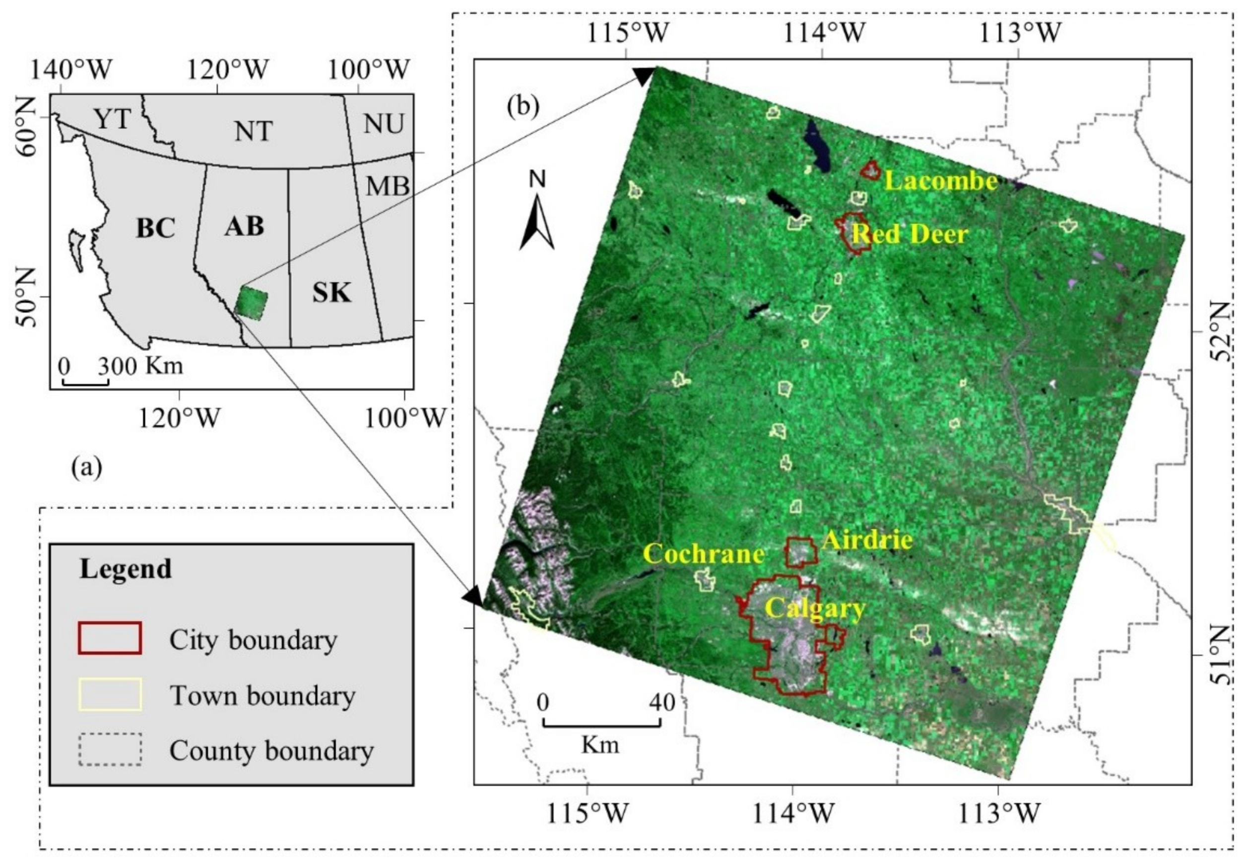
2.1. General Description of the Study Area

In this study, we considered the southern part of the province of Alberta, Canada, as our study area. The area consists of a major city, Calgary, some smaller cities and townships (i.e., Cochrane, Airdrie, and Chestermere), and some rural areas within the single image captured through the Landsat-8 OLI satellite. The area covers approximately 37,772 km² and comprises built up areas, agricultural land, forests, and water bodies (see Figure 1 for details). Climatically, this area is cold, i.e., annual average temperature in the range of −3.6 to 1.1 °C; and dry, i.e., annual average precipitation varies between 377–535 mm [34].

2.2. Data Requirements and Pre-Processing

In this study, we employed several datasets, such as: (i) MODIS-based air temperature normal maps from the time periods 1961–1990 and 1981–2010 at 1 km spatial resolution (Figure 2; incorporating the results of calibrated models and validation) [12]; (ii) Landsat-derived NDVI images at 15 m spatial resolution; and (iii) MODIS-derived 16-day composite vegetation indices that included EVI, and NDVI at 250 m spatial resolution during the year 2004 and 2008 (see

Table 1. Different datasets used in this study.

Satellite Sensor	Data Type	Spatial Resolution	Period/Date	Description	Source
MODIS	MODIS-derived Air Temperature Normal	1 km	Periods 1961–1990, and 1981–2010	Transformed MODIS-derived surface temperature (i.e., 8-day composite of land surface temperature, MOD11A2 v.005) into air temperature normal.	[12]
Landsat-8 OLI	NDVI	15 m	04-Aug-2013, 10-Jul-2014, 11-Aug-2014, 27-Jun-2015.	Pan-sharpened NDVI by using multispectral (MS: red and NIR) bands, and Panchromatic (PAN) band	[34]
MODIS	NDVI and EVI	250 m	Years 2004 and 2008	16-day composite (i.e., MOD13Q1 v. 006)	NASA

). For validation purposes, we opted to use this previously generated data set at 1 sq. km. spatial resolution (Figure 2) [12]. Brief descriptions of these datasets and the corresponding pre-processing involved are found in the following sub-sections.

2.2.1. MODIS-Based Air Temperature Normal Data (i.e., 1 × 1 km²)

For the purpose of this study, we considered ‘air temperature normal’ as the average observed temperature over a 30 year time period that was considered in the contemporary literature and by major climate-related research organizations [35,36,37,38]. The periods we used to calculate the normal air temperature were as follows: (i) 1961–1990; (ii) 1971–2000; and (iii) 1981–2010. The data were collected at several climatological stations across the province of Alberta that followed the World Meteorological Organization (WMO) standard.

In our earlier study [12], we developed methods to delineate normal air temperature at 1 km spatial resolution, which was available for this study. In this process, there were three distinct steps. Firstly, we compared the annual average air temperature over the period 2001–2010 with the normal air temperature during the periods 1961–1990 and 1981–2010 for the five major urban centers in Alberta (i.e., Edmonton, Red Deer, Calgary, Lethbridge, and Medicine Hat). Such comparisons were accomplished by generating a co-efficient of determination (r² values), root mean square error (RMSE), and linear regression analysis. Secondly, we finalized the specific year that demonstrated higher r² and lower RMSE values to acquire MODIS-based satellite images (i.e., eight-day composite land surface temperature images at 1 km spatial resolution, MOD11A2 v.005). In this case, we observed a strong correlation between the annual average air temperature of 2004 with the air temperature normal 1981–2010 (r² = 0.98, and RMSE = 0.25), and again between the annual average air temperature of 2008 with the air temperature normal 1961–1990 (r² = 0.94, and RMSE = 0.51) [12]. Once the MODIS-derived satellite data were acquired, we pre-processed the 8-days composite images; evaluated the quality of the pixels using quality control information; and subsequently eliminated the null pixels by adopting an algorithm described in Hassan et al. [39]. Upon the completion of these stages, we finally transformed the MODIS-derived surface temperature into the normal air temperature. Then we validated the data based on information acquired from climatic stations distributed spatially within the province of Alberta; and found a reasonable agreement (i.e., r² ≈ 0.80; and RMSE ≈ 0.63) between them.

2.2.2. Landsat-8 OLI-derived NDVI Data at 15 m Spatial Resolution

We obtained a Landsat-derived NDVI image at 15 m spatial resolution, which was developed in one of our earlier studies [34]. The method of processing these data consisted of two major steps: (i) collecting the Landsat-8 OLI data and comparing the relationships between multi-spectral (MS) (red and NIR spectral bands at 30 m) and panchromatic (PAN) bands at 15 m; and consequently, determining their suitability to enhance the spatial resolution of the MS bands; and (ii) generating the NDVI at 15 m spatial resolution. We observed significant relationships between the red and PAN bands (i.e., the r² values were 0.84-0.96 for approximately 95% of the pixels), and weaker relationships between the NIR and PAN bands (i.e., r² values were approximately 0.53) [34]. The weak relation was observed due to the fact that these two bands (i.e., NIR and PAN) do not have overlapping wavelengths [34]. As a result, we resampled the 30 m NIR band into 15 m, and used them in conjunction with the pan-sharpened red band to generate the NDVI at 15 m spatial resolution. It is worth mentioning that comparisons between the NDVI generated at 15 m and 30 m (using the original spatial resolution of Landsat images) revealed strong relationships with a r² of ~0.98 and RMSE ~ 0.01.

In preparing the data for this study, we obtained the Landsat-8 OLI images from the United States Geological Survey (USGS) for specific days in the summer months with minimum cloud contamination. We found that the image captured on August 24 in 2013 was under relatively clear-sky conditions; it was considered for use for generating the NDVI surface at 15 m spatial resolution.

2.2.3. MODIS-Based 16-Day Composite NDVI and EVI Data at 250 m for 2004 and 2008

We obtained the MODIS-based 16-day composite NDVI and EVI data (i.e., MOD13Q1 version 006) at 250 m spatial resolution from NASA for the years 2004 and 2008. Upon downloading the data, we prepared mosaic panels and subsets to the extent of the study area. Also, we re-projected the images into the UTM zone 12 projection system using the datum NAD83. Then, we stored these images and converted them into the Geo-TIFF format for further analysis as input files in this particular research project. We calculated the annual average NDVI ($\overline{\mathit{N}\mathit{D}\mathit{V}\mathit{I}}\mathit{y}$) and EVI ($\overline{\mathit{E}\mathit{V}\mathit{I}}\mathit{y}$) from 16-day composites of 26 images (n = 26) that spanned the entire year of interest (y = 2004 and 2008) using the following expressions:

$$\overline{\mathit{N}\mathit{D}\mathit{V}\mathit{I}}\mathit{y}\mathbf{=}{\displaystyle \mathbf{\sum }}_{\mathit{i}\mathbf{=}\mathit{1}}^{\mathit{n}}\mathit{N}\mathit{D}\mathit{V}\mathit{I}\mathbf{/}\mathit{n}$$

(1)

$$\overline{\mathit{E}\mathit{V}\mathit{I}}\mathit{y}\mathbf{=}{\displaystyle \mathbf{\sum }}_{\mathit{i}\mathbf{=}\mathit{1}}^{\mathit{n}}\mathit{E}\mathit{V}\mathit{I}\mathbf{/}\mathit{n}$$

(2)

3. Methods

Figure 3 illustrates the schematic diagram for generating a high spatial resolution local warming map at 15 m during 1961–2010. The methods consisted of three main components: (i) exploring the relationships between air temperature and vegetation indices; (ii) generating the long-term annual average vegetation indices that are considered in this particular research; and (iii) generating local warming maps at high spatial resolution for the 1961–2010 time period. Explanations of these consistent methods are discussed hereafter.

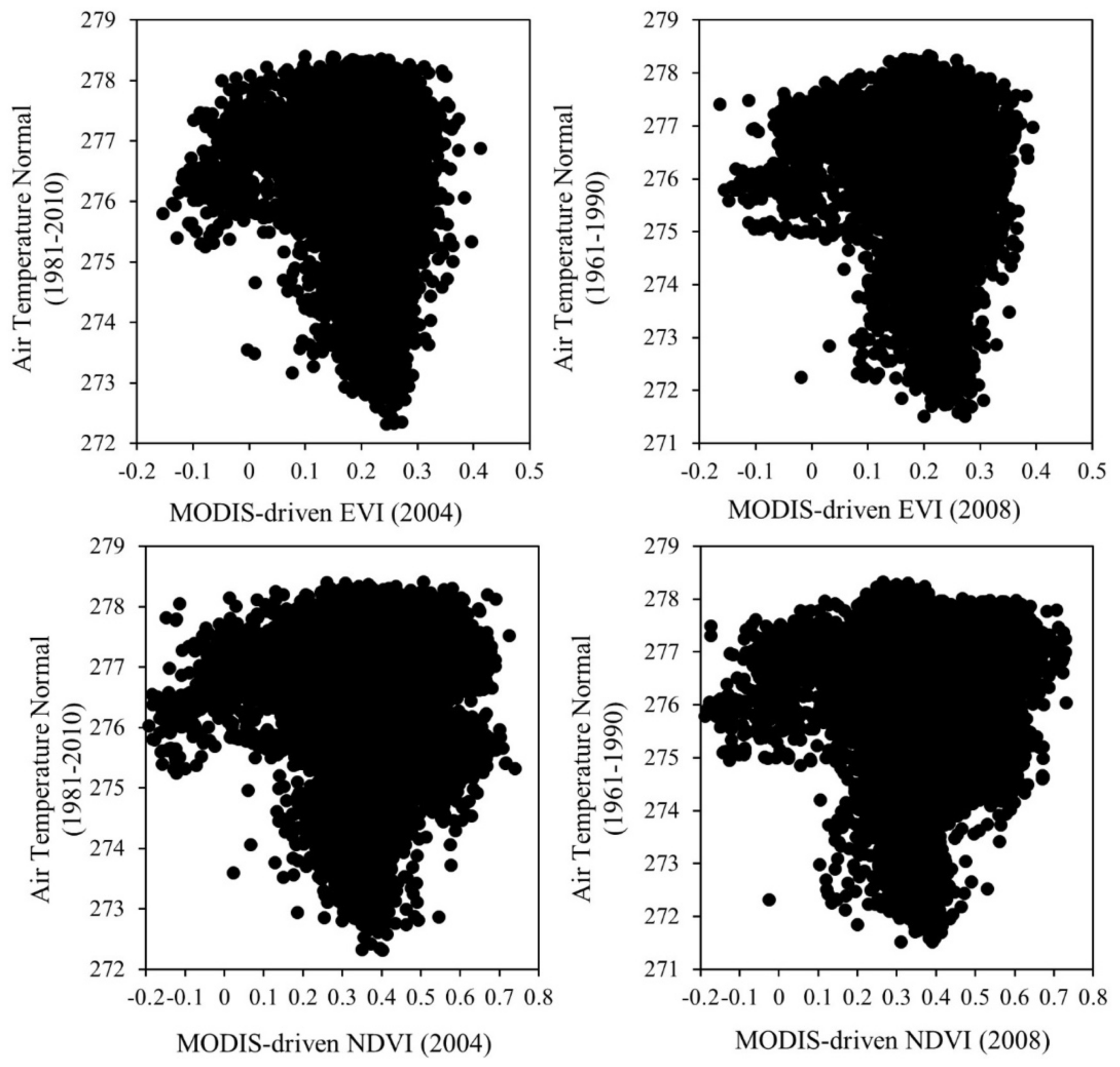
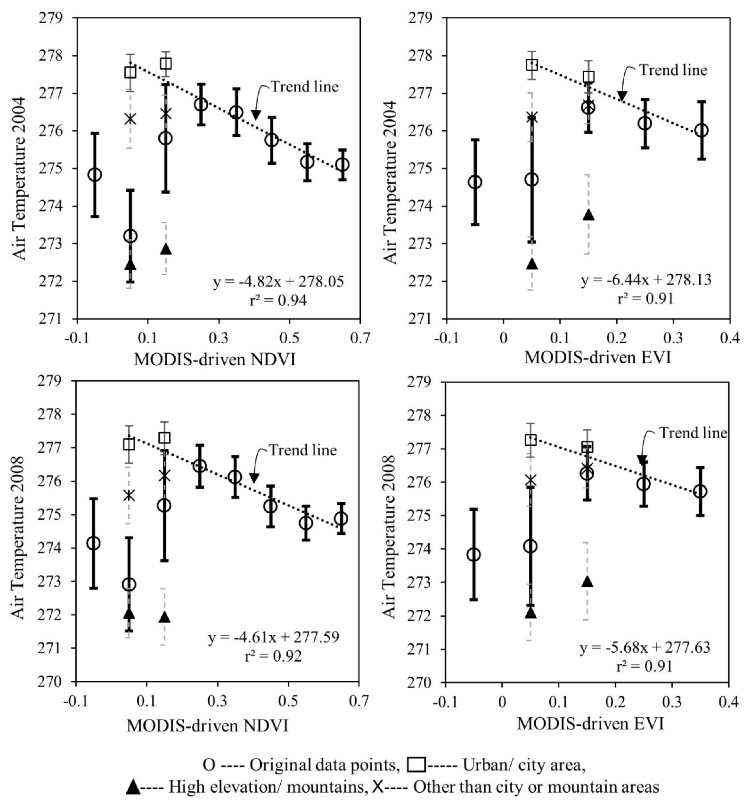
3.1. Exploring Relationships Between MODIS-Derived Annual Air Temperature Normals and Annual Average Vegetation Indices

Once we collected and pre-processed the acquired images as described in the previous section (Section 2), we started to assess the relationships between the normal air temperatures and annual average vegetation indices (i.e., EVI and NDVI). Upon compiling the data into scatter plots (see Figure 4 for details), we observed that the data were sparsely distributed and did not follow any specific pattern of relationship between the variables of interest. It is common to observe an inverse relationship (i.e., when air temperature increased, the EVI or NDVI eventually decreased) between the temperature and vegetation indices [40]; thus, we opted to introduce the technique of binning for the vegetation indices and calculate the corresponding average normal air temperature values. In such cases, it might be possible that lower amount of vegetation with NDVI values in the range of 0 to 0.2 over high altitudes and in the vicinity of marshy/swamp lands would not exhibit inverse relationships as assumed earlier. This would be the case as both high altitudes and marshy/swamp lands (with a presence of relatively more water) would exhibit lower temperature regimes that would be unfavorable for vegetation growth. Upon examining these relationships, we determined the effective vegetation index (i.e., NDVI in this study, see Figure 5 for details) that would have concealed better relations with the air temperature normal regimes (see details in the results and discussion section).

3.2. Generating Long-Term Annual Average NDVI at 15 m Spatial Resolution

Upon building the relationships between the annual average NDVI and normal air temperature, we opted to calculate a long-term average of NDVI values ($\mathit{N}\mathit{D}\mathit{V}{\mathit{I}}_{\mathit{L}\mathit{o}\mathit{n}\mathit{g}\mathbf{-}\mathit{t}\mathit{e}\mathit{r}\mathit{m}}$) at 15 m spatial resolution using the following consecutive steps described in Hassan et al. [33]:

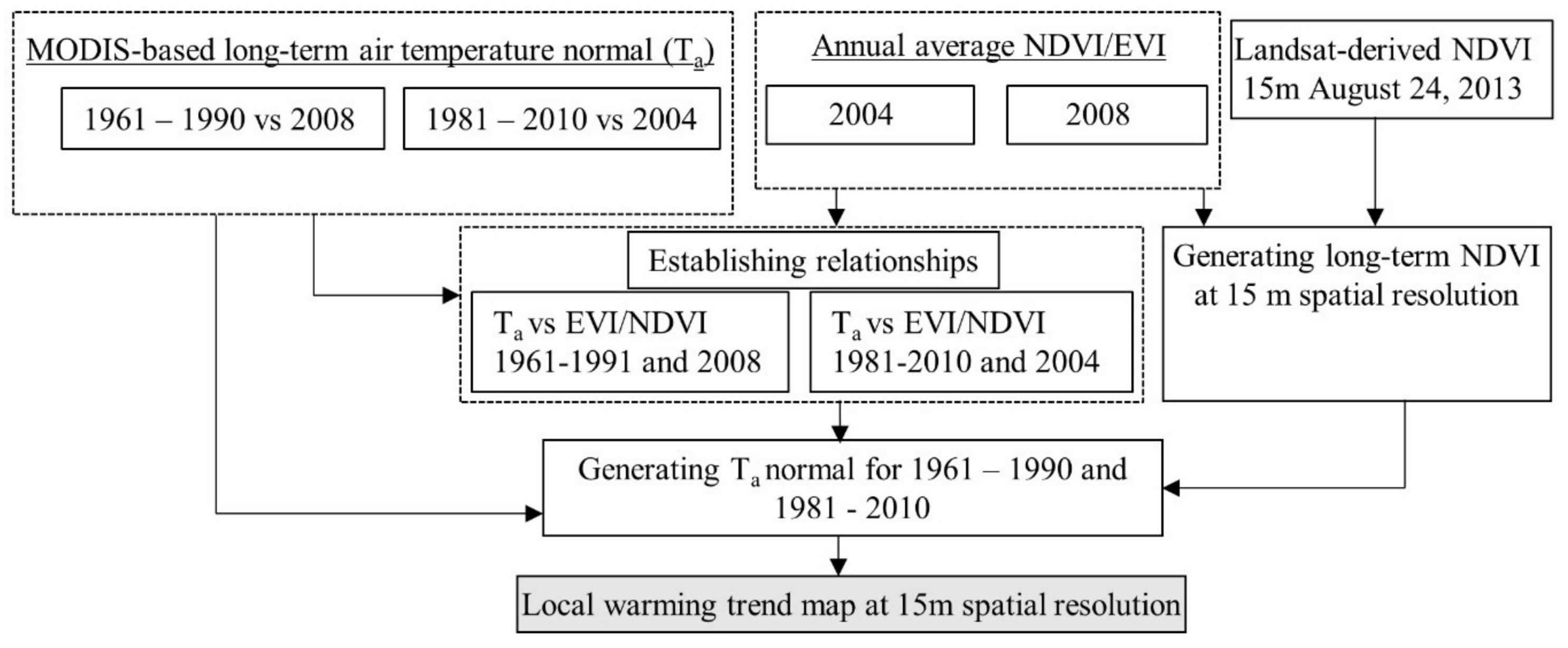
• Used MODIS-based NDVI products to compute the pixel-level average of the annual NDVI for the years 2004 and 2008 at 250 m spatial resolution, as in Equation (1). Then we computed a single NDVI value (i.e., ${\overline{\mathit{N}\mathit{D}\mathit{V}\mathit{I}}}_{\mathit{M}\mathit{O}\mathit{D}\mathit{I}\mathit{S}}$) by spatially averaging the NDVI average pixels of the whole year.
• Calculated the Landsat-8 OLI scene specific spatial average of NDVI (${\overline{\mathit{N}\mathit{D}\mathit{V}\mathit{I}}}_{\mathit{L}\mathit{a}\mathit{n}\mathit{d}\mathit{s}\mathit{a}\mathit{t}\mathbf{-}\mathbf{8} \mathit{O}\mathit{L}\mathit{I}}$); and
• Finally, derived the ($\mathit{N}\mathit{D}\mathit{V}{\mathit{I}}_{\mathit{L}\mathit{o}\mathit{n}\mathit{g}\mathbf{-}\mathit{t}\mathit{e}\mathit{r}\mathit{m}}$) at 15 m spatial resolution using Equation (3), where the difference between the ${\overline{\mathit{N}\mathit{D}\mathit{V}\mathit{I}}}_{\mathit{L}\mathit{a}\mathit{n}\mathit{d}\mathit{s}\mathit{a}\mathit{t}\mathbf{-}\mathbf{8} \mathit{O}\mathit{L}\mathit{I}}$ and ${\overline{\mathit{N}\mathit{D}\mathit{V}\mathit{I}}}_{\mathit{M}\mathit{O}\mathit{D}\mathit{I}\mathit{S}}$ was used as a correction factor for the Landsat-8 OLI based NDVI values.

  $$\mathit{N}\mathit{D}\mathit{V}{\mathit{I}}_{\mathit{L}\mathit{o}\mathit{n}\mathit{g}\mathbf{-}\mathit{t}\mathit{e}\mathit{r}\mathit{m}}\mathbf{=}\mathit{N}\mathit{D}\mathit{V}{\mathit{I}}_{\mathit{L}\mathit{a}\mathit{n}\mathit{d}\mathit{s}\mathit{a}\mathit{t}\mathbf{-}\mathbf{8} \mathit{O}\mathit{L}\mathit{I}}\text{−}\mathbf{(}{\overline{\mathit{N}\mathit{D}\mathit{V}\mathit{I}}}_{\mathit{L}\mathit{a}\mathit{n}\mathit{d}\mathit{s}\mathit{a}\mathit{t}\mathbf{-}\mathbf{8} \mathit{O}\mathit{L}\mathit{I}}\text{−}{\overline{\mathit{N}\mathit{D}\mathit{V}\mathit{I}}}_{\mathit{M}\mathit{O}\mathit{D}\mathit{I}\mathit{S}}\mathbf{)}$$

  (3)

Note that the NDVI values we derived from both the Landsat-8 OLI and MODIS sources were atmosphere-corrected. In both cases, the MODIS and Landsat-8 OLI systems conducted solar spectrum vector (i.e., 6SV) atmospheric correction methods [41]. As a result, we did not opt to apply any further procedure to pursue atmospheric corrections for the data sets.

3.3. Generating Local Warming Maps at 15 m Spatial Resolution

In order to enhance the spatial resolution of the normal air temperature at 15 m, we adapted the data fusion technique described and implemented in Hassan et al. [33] and Hassan and Bourque [42]. We directed this method by generating an artificial image plane (AI) based on instantaneous values ($\mathit{N}\mathit{D}\mathit{V}{\mathit{I}}_{\mathit{i}\mathit{n}\mathit{s}\mathit{t}\mathit{a}\mathit{n}\mathit{t}\mathit{a}\mathit{n}\mathit{e}\mathit{o}\mathit{u}\mathit{s}}$) and an average of the long-term NDVI values ($\mathit{N}\mathit{D}\mathit{V}{\mathit{I}}_{\mathit{a}\mathit{v}\mathit{e}\mathit{r}\mathit{a}\mathit{g}\mathit{e}}$) over a 3 × 3 moving window as described in Section 3.2 by plugging them in the following equation:

$$\mathit{A}\mathit{I}\mathbf{=}\frac{\mathit{N}\mathit{D}\mathit{V}{\mathit{I}}_{\mathit{a}\mathit{v}\mathit{e}\mathit{r}\mathit{a}\mathit{g}\mathit{e}}}{\mathit{N}\mathit{D}\mathit{V}{\mathit{I}}_{\mathit{i}\mathit{n}\mathit{s}\mathit{t}\mathit{a}\mathit{n}\mathit{t}\mathit{a}\mathit{n}\mathit{e}\mathit{o}\mathit{u}\mathit{s}}}$$

(4)

Note that the AI may be considered an index that defines the relation of an instantaneous NDVI value to the average NDVI value of the surrounding pixels. In comparison to Hassan et al. [33], and Hassan and Bourque [42], we swapped the average and instantaneous values of NDVI in order to observe an overall negative relationship (see Figure 5 in the results and discussion section for details). Also, the AI values over water bodies (when the NDVI < 0) and high altitude and marshy lands with NDVI values from 0 to 0.2, were assumed to be 1 in order to maintain the same level of normal air temperature values. Thus, once the AI values were obtained, we then converted the normal air temperature ${\mathit{T}}_{{\mathit{a}}_{normal @ 1 km}}$ values into their equivalent at 15 m ${\mathit{T}}_{{\mathit{a}}_{normal @ 15 m}}$ using the following expressions:

$${\mathit{T}}_{{\mathit{a}}_{normal @ 15m}}=\mathrm{AI}\times {\mathit{T}}_{{\mathit{a}}_{normal @ 1km}}$$

(5)

Once we generated the normal air temperatures (i.e., 1961–1990 and 1981–2010) at 15 m spatial resolution, we then compared the normal maps spawned at 1 km spatial resolution in the scope of an earlier study [12] with the correlation coefficient (r²) and RMSE. Finally, we produced difference maps of two climate normals to perceive local warming trends over the study area at 15 m spatial resolution.

4. Results and Discussion

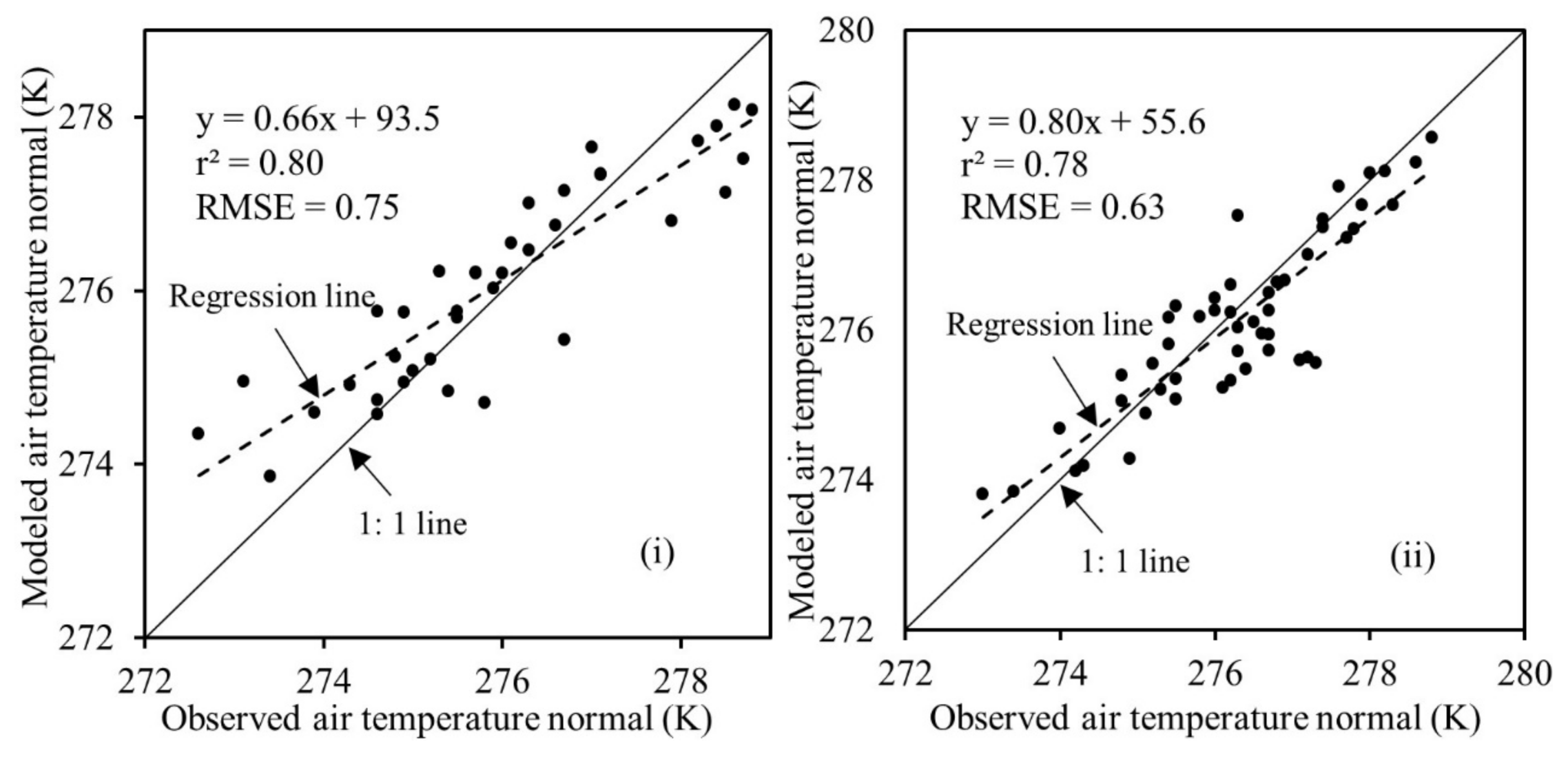
4.1. Relationship Between MODIS-Based Normal Air Temperature and VI

Figure 4 represents the scatter plots of MODIS-driven VI (year specific) and normal air temperatures (i.e., 1961–1990; and 1981–2010). It displayed no relationships between the variables of interest. As a result, we decided to introduce the binning technique of data analysis to re-arrange the scatter plots into several divisions so that the relationships might closely be observed as illustrated in Figure 5. It exhibited a negative relation with the air temperature normal when the VI values were greater than 0.2 in particular, which would be common to find in the literature [22,32,40,43,44,45,46]. Also, we did not observe such a generic relation between the variables of interest for the NDVI/EVI values in the range −0.1 to 0.2. Consequently, we decided to introduce the masking technique (see detail in the methods section) and recalculated the VI values against the air temperature normal for the −0.1 to 0.2 range. Intriguingly, the outcome of this analysis revealed a negative slope and strong correlation between NDVI/EVI and the air temperature values. We achieved r² values of: (i) 0.94, and 0.92 for NDVI (in the year 2004 and 2008, respectively); and (ii) 0.91 for EVI (in both 2004 and 2008) and a negative slope while comparing with air temperature.

As we did not find a negative relationship between the VI and normal air temperature up to a certain range (Figure 5), we assumed that it might have been due to the existence of sparse vegetation over elevated lands or in the vicinity of water bodies in the study area. It is worth noting that our study area contains rocky mountain areas and few sporadically-distributed water bodies. As a result, the binning technique was helpful to investigate the impact of such landscapes in our study area, and to perceive the dynamic relationships between VI and air temperature. Consequently, it was quite natural to see that the relationship did not exhibit a general pattern (i.e., higher NDVI values would demonstrate lower air temperature) according to scientific notions. Hence, introducing the binning technique in this analysis was found to be unique in characterizing the landscapes and vegetation covers to recognize the fact that mountainous areas would have lower air temperature with little green vegetation on top. Additionally, water bodies and surrounded swamp/marshy lands would demonstrate lower to negative NDVI values. Therefore, we ignored the negative EVI/NDVI values as they generally revealed water bodies in the study area. The other two bin classes with relatively lower EVI/NDVI values (>0.0 to 0.1, and >0.1 to 0.2) were ignored once we observed them over high altitude, and found them to be other than city areas (i.e. marshy or swamp areas). Upon pursuing these processes, we observed that the relationships between EVI/NDVI and normal air temperature demonstrated the usual schemas mentioned in the relevant literature [22,24,32,40,43,44,45,46].

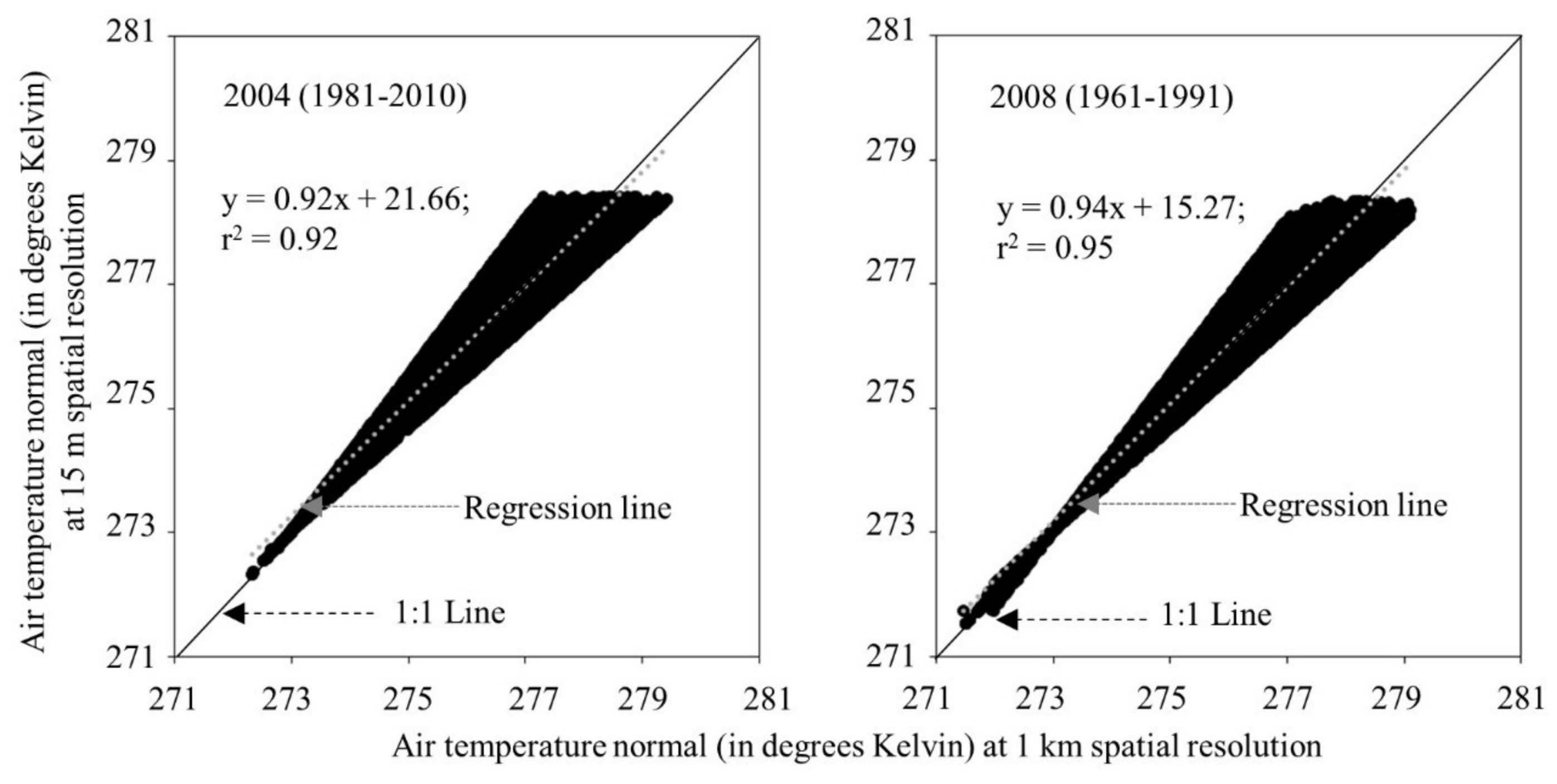
4.2. Generating Normal Air Temperatures and Local Warming Maps at 15 m Spatial Resolution

As we obtained significant relationships between the air temperature normal and NDVI (see Figure 5) after introducing the binning technique, we decided to enhance the spatial resolution of the air temperature normal maps. We then executed the algorithm introduced in the methods section to generate the air temperature normal for each climate normal (i.e., 1961–1990; and 1981–2010). Upon producing the air temperature normal maps at 15 m spatial resolution for each climate normal individually, we compared the generated maps with the 1 km spatial resolution map developed in earlier research [12]. Figure 6 shows the comparison of normal air temperatures at 15 m and 1 km spatial resolution. Once we compared the normal air temperature of 1981–2010, represented by a yearly average air temperature of 2004 at 15 m spatial resolution with that of the 1 km spatial resolution, we found a strong correlation (i.e., r² = 0.92; slope = 0.92; and intercept = 21.66). The relationship was almost identical when comparing the similar data sets obtained for the 1961–1990 normal temperature for the 15 m and 1 km spatial resolution (i.e., r² = 0.95; slope = 0.94; and intercept = 15.27).

Note that in the case of the 1 km spatial resolution warming map, we used 80% of the ground-based dataset for model calibration and the remaining 20% dataset for validation, as shown in Figure 2. Also, we evaluated the multiple partitioning of the entire ground-based data so that the spatial distribution of the ground stations might be representative. We employed the Geospatial Modeling Environment (GME) technique to evaluate the bivariate uniform random distribution using the feature space, raster space, and extent in order to define whether a given data-point would fall within a particular rectangular boundary of interest. As a result, we used the already-developed 1 km spatial resolution warming map to validate the newly-developed 15 m resolution warming map, because: (i) the prior datasets were scientifically validated based on the observations of the ground stations for the entire province of Alberta; (ii) the present study area contained only five weather stations that captured long-term temperature data maintaining WMO standards, and thus it would not be appropriate to use such a minimal number of representative data points; (iii) the ground stations within the present study area were highly concentrated in urban areas and might not be representative for our study area; and (iv) there was a lack of long-term temperature data at the ground stations, and thus the development of a remote-sensing based model would be critical.

Figure 7 shows the warming trend map (i.e., the difference between the normal air temperature maps of 1961–1990 and 1981–2010) generated at 15 m spatial resolution. It shows that around 58% of the study area has undergone an increased temperature shift (i.e., from 0.25 °C to greater than 1 °C; see yellow, orange, deep orange, and red color in Figure 7 for details). Additionally, about 38% of areas encountered almost no change of air temperature (i.e., in the range of −0.25 °C to +0.25 °C; as seen in yellowish green, and green color in Figure 7). On the contrary, around 4% of the total area had endured a minor cooling trend (i.e., less than -0.25 °C). In this case, our calculated average increase of air temperature in the study area was 0.34 °C, with a standard deviation ± 0.36 °C. Canada as a whole gained an average warming of 1.4 °C during the period 1948–2009, and the Canadian Prairie underwent an average regional warming between 0.9 to 1.7 °C [36]. These national and regional estimates of air temperature change used similar methods as those comparing the modeled air temperature reported in this study. However, the observed difference might be due to the fact that the temperature in local areas (i.e., 15 m spatial resolution) would certainly demonstrate different dynamics compared to national, regional, and global models.

It is worth noting that we found an incremental shift in the normal air temperature 1961 to 2010 over most of the study area. Also, we noticed cooling patches in few areas (see Figure 6 in blue color). The pattern of spatial warming trend in our study area might have increased for several reasons, including but not limited to the following.

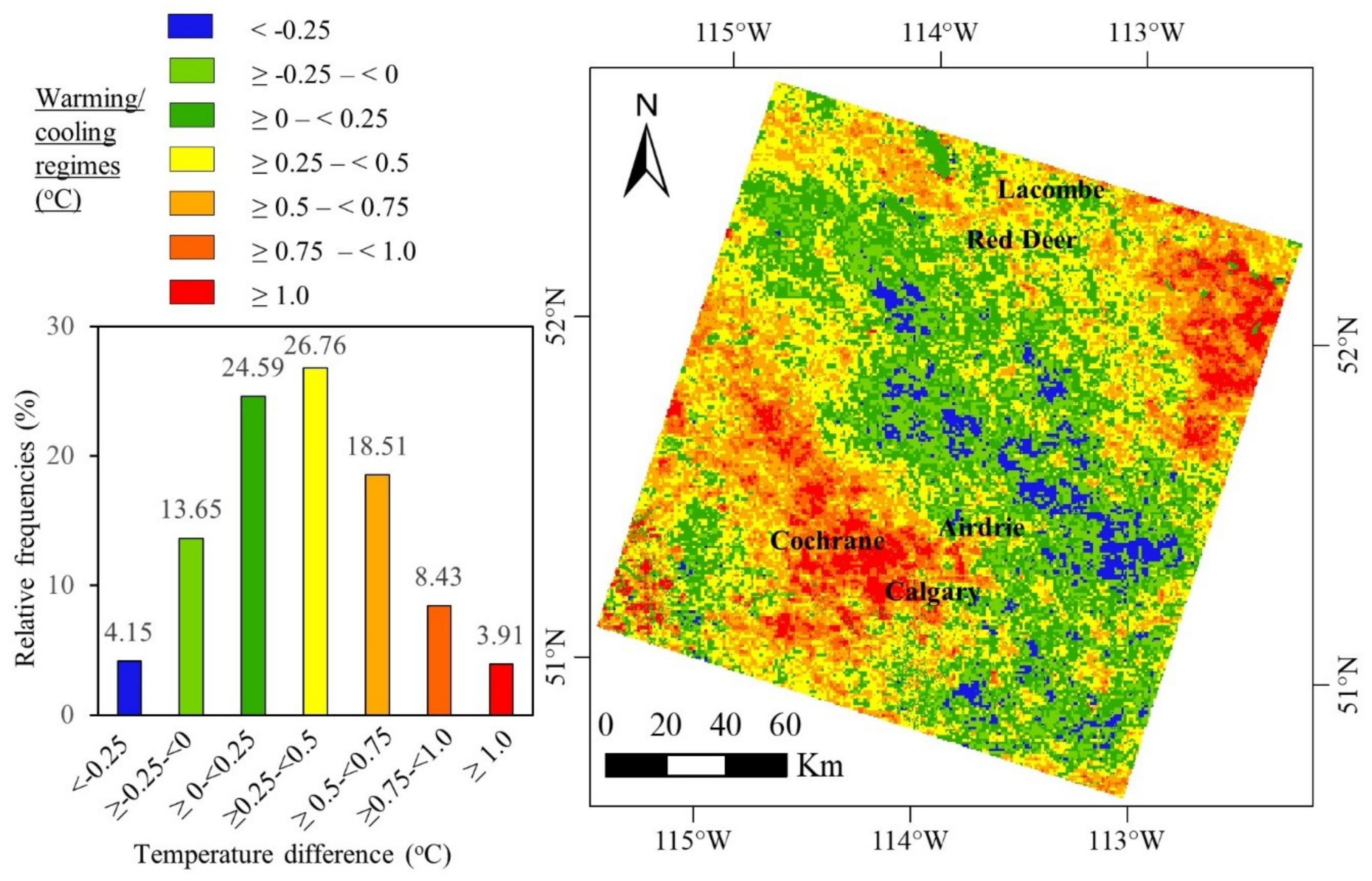
• Rapid urbanization coupled with intense mixed-use development (i.e., industrial/residential; or community/residential development) [47], and brisk conversion of agricultural and forest lands to non-agricultural practices [48] made a significant contribution to the increased temperature regimes in small and major cities in our study area including Calgary, Red Deer, Cochrane, Airdrie, and Chestermere in particular. Besides, the existence of two major cities in Alberta (i.e., Calgary, and Red Deer) in the study area might have had a direct influence on the extent of the built environment, population density, anthropogenic activities, and socio-economic aspects (i.e., tourism activities) to contribute to augmenting the warming trends in and outside the city boundaries. Additionally, the fastest growing corridor of Alberta (i.e., the Calgary–Edmonton corridor), with an approximate area of about 40,000 km², stretching north from Calgary through Red Deer to Edmonton, has experienced an increase in population escalation since the 1980s and was home to almost 75% of the population of Alberta in 2011 [49]. Our study area covered significant belts of this corridor and we assumed that the rapid urbanization and industrial growth in this particular region might have had a direct influence on the increased normal temperature during the 1961–2010 time period;
• The North-Eastern part of our study area experienced a temperature increase of around 1 °C. This area is primarily dominated by agricultural land use near the City of Red Deer. Additionally, being the third largest producer of agri-food products in Canada [50], Alberta experienced unprecedented pressure of development in private agricultural and economic growth (i.e., an average growth of 3.5% nationally) [50], which might affect the shift of temperature changes in this specific region;
• In the South-Western part (Figure 6), there is the presence of the Rocky Mountain Areas (Kananaskis county and Banff National Park) that experienced an increase temperature during the 1961–2010 time period. This might have occurred due to the continuous development of tourism activities [51], and relevant accomplishments (i.e., infrastructure development, catering services, and transportation services);
• The cooling trends in very few areas (blue patches in Figure 6) in the middle of our study area were discerned and might have a direct relation to existence of waterbodies and forested lands. However, it is critical to note that the representation of such a negative temperature shift (i.e., cooling trend in this case) only accounted for around 4% (i.e., an insignificant amount) of the total study area and were sparsely distributed throughout the warming trend map.

5. Concluding Remarks

Within the scope of this study, we demonstrated a remote sensing-based modelling framework for local warming trends at 15 m spatial resolution. The proposed methods involved (i) the construction of high resolution EVI and NDVI maps at 15 m spatial resolution; (ii) comprehending the 1 km resolution air temperature map available from a previous study using the higher resolution VI maps; and (iii) the generation of local warming map at 15 m spatial resolution as a final product. Remarkably, the study discovered that approximately 58% of the areas experienced a somewhat increased temperature and approximately 38% did not show any significant change. However, around 4% of areas underwent a cooling trend. Moreover, we compared the outcome of this study with the normal temperatures developed at 1 km spatial resolution. The results revealed strong relationships (i.e., r² = 0.95 for 1961–1990; and r² = 0.92 for the 1981–2010 normal temperature) and exhibited similar patterns of temperature change throughout the study area. However, challenges still remained regarding obtaining long-term temperature datasets through the ground-based stations to validate the model outcomes. In this context, we recommend that prior to using this method for enhanced spatial resolution warming maps, researchers or practitioners should also consider the availability of ground-based temperature data that comply with international standards. Apart from this, the scientific methods that we adopted to generate local warming maps at a high spatial resolution using remote sensing data (i.e., air temperature and vegetation indices) are critical to recognizing local warming trends at the community level. Consequently, this research outcome provides advantageous information for smaller cities and communities in preparing climate-related risks and adaptation planning in their own jurisdictional areas. For this specific study, we implemented our model in and around the city of Calgary. Finally, if the scientific community and practitioners are interested in deploying this model in their own communities, we recommend that the method should be evaluated thoroughly prior to application in other parts of the world.

References

1. Jones, P.D.; Lister, D.H.; Osborn, T.J.; Harpham, C.; Salmon, M.; Morice, C.P. Hemispheric and large-scale land-surface air temperature variations: An extensive revision and an update to 2010. J. Geophys. Res. Atmos. 2012, 117. [Google Scholar] [CrossRef] [Green Version]
2. Harris, I.; Jones, P.D.; Osborn, T.J.; Lister, D.H. Updated high-resolution grids of monthly climatic observations - the CRU TS3.10 Dataset. Int. J. Climatol. 2014, 34, 623–642. [Google Scholar] [CrossRef] [Green Version]
3. Menne, M.J.; Williams, C.N.; Palecki, M.A. On the reliability of the U.S. surface temperature record. J. Geophys. Res. Atmos. 2010, 115, 1–9. [Google Scholar] [CrossRef]
4. Vanderbei, R.J. Local Warming. SIAM Rev. 2012, 54, 597–606. [Google Scholar] [CrossRef] [Green Version]
5. Mahlstein, I.; Hegerl, G.; Solomon, S. Emerging local warming signals in observational data. Geophys. Res. Lett. 2012, 39, 1–5. [Google Scholar] [CrossRef]
6. Seto, K.C.; Guneralp, B.; Hutyra, L.R. Global forecasts of urban expansion to 2030 and direct impacts on biodiversity and carbon pools. Proc. Natl. Acad. Sci. USA 2012, 109, 16083–16088. [Google Scholar] [CrossRef] [PubMed] [Green Version]
7. Trlica, A.; Hutyra, L.R.; Schaaf, C.L.; Erb, A.; Wang, J.A. Albedo, Land Cover, and Daytime Surface Temperature Variation Across an Urbanized Landscape. Earth’s Future 2017, 5, 1084–1101. [Google Scholar] [CrossRef] [Green Version]
8. Bren d’Amour, C.; Reitsma, F.; Baiocchi, G.; Barthel, S.; Güneralp, B.; Erb, K.-H.; Haberl, H.; Creutzig, F.; Seto, K.C. Future urban land expansion and implications for global croplands. Proc. Natl. Acad. Sci. USA 2016, 114, 8939–8944. [Google Scholar] [CrossRef] [PubMed] [Green Version]
9. Antrop, M. Landscape change and the urbanization process in Europe. Landsc. Urban Plan. 2004, 67, 9–26. [Google Scholar] [CrossRef]
10. Shrestha, M.K.; York, A.M.; Boone, C.G.; Zhang, S. Land fragmentation due to rapid urbanization in the Phoenix Metropolitan Area: Analyzing the spatiotemporal patterns and drivers. Appl. Geogr. 2012, 32, 522–531. [Google Scholar] [CrossRef]
11. Rizwan, A.M.; Dennis, L.Y.C.; Liu, C. A review on the generation, determination and mitigation of Urban Heat Island. J. Environ. Sci. 2008, 20, 120–128. [Google Scholar] [CrossRef]
12. Rahaman, K.R.; Hassan, Q.K.; Chowdhury, E.H. Quantification of Local Warming Trend: A Remote Sensing-Based Approach. PLoS ONE 2017, 12, 1–18. [Google Scholar] [CrossRef] [PubMed]
13. New, M.; Lister, D.; Hulme, M.; Makin, I. A high-resolution data set of surface climate over global land areas. Clim. Res. 2002, 21, 1–25. [Google Scholar] [CrossRef] [Green Version]
14. Grimmond, S. Urbanization and global environmental change: Local effects of urban warming. Geogr. J. 2007, 173, 83–88. [Google Scholar] [CrossRef]
15. Mahlstein, I.; Knutti, R.; Solomon, S.; Portmann, R.W. Early onset of significant local warming in low latitude countries. Environ. Res. Lett. 2011, 6, 034009. [Google Scholar] [CrossRef]
16. Benas, N.; Chrysoulakis, N.; Cartalis, C. Trends of urban surface temperature and heat island characteristics in the Mediterranean. Theor. Appl. Climatol. 2017, 130, 807–816. [Google Scholar] [CrossRef]
17. Lazzarini, M.; Marpu, P.R.; Ghedira, H. Temperature-land cover interactions: The inversion of urban heat island phenomenon in desert city areas. Remote Sens. Environ. 2013, 130, 136–152. [Google Scholar] [CrossRef]
18. Streutker, D.R. A remote sensing study of the urban heat island of Houston, Texas. Int. J. Remote Sens. 2002, 23, 2595–2608. [Google Scholar] [CrossRef] [Green Version]
19. Liu, L.; Zhang, Y. Urban heat island analysis using the landsat TM data and ASTER Data: A case study in Hong Kong. Remote Sens. 2011, 3, 1535–1552. [Google Scholar] [CrossRef]
20. Yang, C.; He, X.; Yan, F.; Yu, L.; Bu, K.; Yang, J.; Chang, L.; Zhang, S. Mapping the Influence of Land Use/Land Cover Changes on the Urban Heat Island Effect—A Case Study of Changchun, China. Sustainability 2017, 9, 312. [Google Scholar] [CrossRef]
21. Grover, A.; Singh, R.; Singh, B.R. Analysis of Urban Heat Island (UHI) in Relation to Normalized Difference Vegetation Index (NDVI): A Comparative Study of Delhi and Mumbai. Environments 2015, 2, 125–138. [Google Scholar] [CrossRef] [Green Version]
22. Zakšek, K.; Oštir, K. Downscaling land surface temperature for urban heat island diurnal cycle analysis. Remote Sens. Environ. 2012, 117, 114–124. [Google Scholar] [CrossRef]
23. Senanayake, I.P.; Welivitiya, W.D.D.P.; Nadeeka, P.M. Remote sensing based analysis of urban heat islands with vegetation cover in Colombo city, Sri Lanka using Landsat-7 ETM+ data. Urban Clim. 2013, 5, 19–35. [Google Scholar] [CrossRef]
24. Ning, J.; Gao, Z.; Meng, R.; Xu, F.; Gao, M.; Deng, Y.; Wang, S.; Bai, X.; Tian, Y.; Wu, L.; et al. Relationship among land surface temperature and LUCC, NDVI in typical karst area. Sci. Rep. 2018, 8, 1–13. [Google Scholar]
25. Chen, X.L.; Zhao, H.M.; Li, P.X.; Yin, Z.Y. Remote sensing image-based analysis of the relationship between urban heat island and land use/cover changes. Remote Sens. Environ. 2006, 104, 133–146. [Google Scholar] [CrossRef]
26. Bechtel, B.; Alexander, P.; Böhner, J.; Ching, J.; Conrad, O.; Feddema, J.; Mills, G.; See, L.; Stewart, I. Mapping Local Climate Zones for a Worldwide Database of the Form and Function of Cities. ISPRS Int. J. Geo-Inf. 2015, 4, 199–219. [Google Scholar] [CrossRef] [Green Version]
27. Weng, Q. Remote sensing of impervious surfaces in the urban areas: Requirements, methods, and trends. Remote Sens. Environ. 2012, 117, 34–49. [Google Scholar] [CrossRef]
28. Mackey, C.W.; Lee, X.; Smith, R.B. Remotely sensing the cooling effects of city scale efforts to reduce urban heat island. Build. Environ. 2012, 49, 348–358. [Google Scholar] [CrossRef]
29. Cao, X.; Onishi, A.; Chen, J.; Imura, H. Quantifying the cool island intensity of urban parks using ASTER and IKONOS data. Landsc. Urban Plan. 2010, 96, 224–231. [Google Scholar] [CrossRef]
30. Haldar, D.; Nigam, R.; Patnaik, C.; Dutta, S.; Bhattacharya, B. Remote sensing-based assessment of impact of Phailin cyclone on rice in Odisha, India. Paddy Water Environ. 2016, 14, 451–461. [Google Scholar] [CrossRef]
31. Darrel Jenerette, G.; Harlan, S.L.; Stefanov, W.L.; Martin, C.A. Ecosystem services and urban heat riskscape moderation: Water, green spaces, and social inequality in Phoenix, USA. Ecol. Appl. 2011, 21, 2637–2651. [Google Scholar] [CrossRef] [PubMed]
32. Hamdi, R. Estimating urban heat island effects on the temperature series of Uccle (Brussels, Belgium) using remote sensing data and a land surface scheme. Remote Sens. 2010, 2, 2773–2784. [Google Scholar] [CrossRef]
33. Hassan, Q.K.; Bourque, C.P.; Meng, F.-R. Application of Landsat-7 ETM+ and MODIS products in mapping seasonal accumulation of growing degree days at an enhanced resolution. J. Appl. Remote Sens. 2007, 1, 013539. [Google Scholar] [CrossRef]
34. Rahaman, K.R.; Hassan, Q.K.; Ahmed, M.R. Pan-Sharpening of Landsat-8 Images and Its Application in Calculating Vegetation Greenness and Canopy Water Contents. ISPRS Int. J. Geo-Inf. 2017, 6, 168. [Google Scholar] [CrossRef]
35. WMO Technical Regulations. Volume I: General Meteorological Standards and Recommended Practices; Technical Paper; WMO: Geneva, Switzerland, 2017. [Google Scholar]
36. Jeff, F. EnviroStats. EnviroStats 2011, 5, 1–30. [Google Scholar]
37. Wang, T.; Hamann, A.; Spittlehouse, D.L.; Murdock, T.Q. ClimateWNA-high-resolution spatial climate data for western North America. J. Appl. Meteorol. Climatol. 2012, 51, 16–29. [Google Scholar] [CrossRef]
38. Flato, G.M.; Boer, G.J.; Lee, W.G.; McFarlane, N.A.; Ramsden, D.; Reader, M.C.; Weaver, A.J. The Canadian centre for climate modelling and analysis global coupled model and its climate. Clim. Dyn. 2000, 16, 451–467. [Google Scholar] [CrossRef]
39. Hassan, Q.K.; Bourque, C.P.; Meng, F.-R.; Richards, W. Spatial mapping of growing degree days: An application of MODIS-based surface temperatures and enhanced vegetation index. J. Appl. Remote Sens. 2007, 1, 013511. [Google Scholar] [CrossRef]
40. Marzban, F.; Sodoudi, S.; Preusker, R. The influence of land-cover type on the relationship between NDVI–LST and LST-Tair. Int. J. Remote Sens. 2018, 39, 1377–1398. [Google Scholar]
41. Ke, Y.; Im, J.; Lee, J.; Gong, H.; Ryu, Y. Characteristics of Landsat 8 OLI-derived NDVI by comparison with multiple satellite sensors and in-situ observations. Remote Sens. Environ. 2015, 164, 298–313. [Google Scholar] [CrossRef]
42. Hassan, Q.K.; Bourque, C.P.A. Spatial enhancement of MODIS-based images of leaf area index: Application to the boreal forest region of northern Alberta, Canada. Remote Sens. 2010, 2, 278–289. [Google Scholar] [CrossRef]
43. Zhou, W.; Qian, Y.; Li, X.; Li, W.; Han, L. Relationships between land cover and the surface urban heat island: Seasonal variability and effects of spatial and thematic resolution of land cover data on predicting land surface temperatures. Landsc. Ecol. 2014, 29, 153–167. [Google Scholar] [CrossRef]
44. Li, Y.Y.; Zhang, H.; Kainz, W. Monitoring patterns of urban heat islands of the fast-growing Shanghai metropolis, China: Using time-series of Landsat TM/ETM+ data. Int. J. Appl. Earth Obs. Geoinf. 2012, 19, 127–138. [Google Scholar] [CrossRef]
45. Buyantuyev, A.; Wu, J. Urban heat islands and landscape heterogeneity: Linking spatiotemporal variations in surface temperatures to land-cover and socioeconomic patterns. Landsc. Ecol. 2010, 25, 17–33. [Google Scholar] [CrossRef]
46. Li, J.; Song, C.; Cao, L.; Zhu, F.; Meng, X.; Wu, J. Impacts of landscape structure on surface urban heat islands: A case study of Shanghai, China. Remote Sens. Environ. 2011, 115, 3249–3263. [Google Scholar] [CrossRef]
47. Young, D. City status in Alberta. Plan North West 2017, 2, 10–14. [Google Scholar]
48. Wang, H.; Qiu, F.; Ruan, X. Loss or gain: A spatial regression analysis of switching land conversions between agriculture and natural land. Agric. Ecosyst. Environ. 2016, 221, 222–234. [Google Scholar] [CrossRef]
49. Martellozzo, F.; Ramankutty, N.; Hall, R.J.; Price, D.T.; Purdy, B.; Friedl, M.A. Urbanization and the loss of prime farmland: A case study in the Calgary–Edmonton corridor of Alberta. Reg. Environ. Chang. 2014, 15, 881–893. [Google Scholar] [CrossRef]
50. Ruan, X.; Qiu, F.; Dyck, M. The effects of environmental and socioeconomic factors on land-use changes: A study of Alberta, Canada. Environ. Monit. Assess. 2016, 188, 446. [Google Scholar] [CrossRef] [PubMed]
51. Groulx, M.; Lemieux, C.J.; Lewis, J.L.; Brown, S. Understanding consumer behaviour and adaptation planning responses to climate-driven environmental change in Canada’s parks and protected areas: A climate futurescapes approach. J. Environ. Plan. Manag. 2017, 60, 1016–1035. [Google Scholar] [CrossRef]
Figure 1. Representing the study area using a Landsat-8 OLI satellite acquired on 11 August 2014 (panel b) in context of western Canada (panel a). The image is a true color composite image consisting of the spectral bands of blue, green, and red at 30 m spatial resolution; which are passed through the same color-plane of a computer display. Note that the red, yellow, and grey boundaries represent city, small township, and built-up environment, respectively, in panel b.
Ijgi 07 00398 g001
Figure 2. Relationship between modeled (satellite-derived data) and observed (ground station-based temperature data) air temperature normal at 1 sq. km spatial resolution for the years 2004 and 2008 [12].
Ijgi 07 00398 g002
Figure 3. Schematic diagram of the methodology of generating local warming map at 15 m spatial resolution.
Ijgi 07 00398 g003
Figure 4. Scatter plots of the comparison of the normal average air temperature (1 km spatial resolution) and MODIS-driven EVI and NDVI (250 m spatial resolution).
Ijgi 07 00398 g004
Figure 5. Relationships between MODIS-driven air temperature normal (1961–1990; 1981–2010), represented by the year (2008; 2004) and annual average vegetation greenness (EVI and NDVI) of 2008 and 2004.
Ijgi 07 00398 g005
Figure 6. Relationships between air temperature normal 2004 (representing 1981–2010) and 2008 (representing 1961–1991) with 1 km and 15 m spatial resolution. Note that the grey dotted line represents the regression line and the black line represents the 1:1 line.
Ijgi 07 00398 g006
Figure 7. Spatial extent of local warming trends during the period 1961–2010 derived at 15 m spatial resolution.
Ijgi 07 00398 g007