Article

Land Cover Mapping from Remotely Sensed and Auxiliary Data for Harmonized Official Statistics

1
Direção-Geral do Território, 1099-052 Lisbon, Portugal
2
European Commission, Joint Research Centre (JRC), Directorate Space, Security and Migration, Disaster Risk Management Unit, 21027 Ispra (VA), Italy
3
Statistics Portugal, 1000-043 Lisbon, Portugal
4
NOVA Information Management School (NOVA IMS), Universidade Nova de Lisboa, Campus de Campolide, 1070-312 Lisbon, Portugal
*
Author to whom correspondence should be addressed.
ISPRS Int. J. Geo-Inf. 2018, 7(4), 157; https://0-doi-org.brum.beds.ac.uk/10.3390/ijgi7040157
Submission received: 16 February 2018 / Revised: 11 April 2018 / Accepted: 14 April 2018 / Published: 21 April 2018

Abstract

:
This paper describes a general framework alternative to the traditional surveys that are commonly performed to estimate, for statistical purposes, the areal extent of predefined land cover classes across Europe. The framework has been funded by Eurostat and relies on annual land cover mapping and updating from remotely sensed and national GIS-based data followed by area estimation. Map production follows a series of steps, namely data collection, change detection, supervised image classification, rule-based image classification, and map updating/generalization. Land cover area estimation is based on mapping but compensated for mapping error as estimated through thematic accuracy assessment. This general structure was applied to continental Portugal, successively updating a map of 2010 for the following years until 2015. The estimated land cover change was smaller than expected but the proposed framework was proved as a potential for statistics production at the national and European levels. Contextual and structural methodological challenges and bottlenecks are discussed, especially regarding mapping, accuracy assessment, and area estimation.

1. Introduction

Up to date land cover and land use (LCLU) statistics are paramount for policy and decision making and, thus, impact largely on economy and society. For example, LCLU patterns and their change influence the climate [1,2] and concerns on the consequences of climate change are driving high-level international policy, including the establishment of international commitments such as the Paris Climate Agreement [3]. However, the production of LCLU statistics becomes increasingly challenging when cross-border regions, such as political or geographical units formed by autonomous states, are involved, which commonly use their own means and criteria for statistics production. Comparability and assembly of national statistics for wider scales are thus commonly compromised.
Efforts have been made to produce harmonized LCLU statistics across countries. In Europe, for example, national and international authorities have formed a partnership, the European Statistical System (ESS), for the development, production, and dissemination of comparable statistics at the European Union level. The ESS functions as a network in which the European Union authority for statistics, Eurostat, in close cooperation with national statistical authorities, leads the way in the harmonization of statistics.
International cooperation can respond to the difficulty in producing coherent statistics across states. For example, surveys for LCLU statistics are commonly used at various national levels. This is the case of the Land Use and Coverage Area frame Survey (LUCAS), promoted by Eurostat with the objective of identifying LCLU change in the European Union (EU). LUCAS takes place every three years and implements a combined approach of field observations and photo-interpretation assigned to field points. LUCAS surveys are carried out in situ in which a subset of the >1 million points defined by a 2 × 2 km2 grid covering the European Union is visited on the ground [4].
Point-based samples periodically visited in situ and other methods commonly applied for producing statistics, such as questionnaires, provide valuable information. However, there are some limitations, notably the non-exhaustive geographical nature of sampling and the relatively long time of revisit. Thus, the information produced has gaps in space and time, which can be small or great depending on the sampling effort and periodicity. Increasing sample size and periodicity increases the costs to possibly unaffordable levels.
An alternative means of obtaining information on LCLU is mapping. Specifically, mapping from remote sensing has been used to produce information about the Earth’s surface and can inform on the areal extent of LCLU across large areas, up to the entire globe. Dozens of LCLU maps have been produced at global and continental scales [5]. Despite the value of these maps—some of them represent milestones in remote sensing—their use is limited mostly because they have been produced independently and for specific points in time and, thus, lack coherency and continuity [5,6].
Efforts have been made for harmonized LCLU mapping. For example, the CORINE Land Cover (CLC) series of maps is a harmonized representation of the LCLU of most of Europe for the reference years of 1990, 2000, 2006, and 2012 [7]. CLC is partly produced by each individual country and, in most cases, by visual interpretation of remotely sensed data. CLC is coordinated by the European Environmental Agency and all countries follow common guidelines to ensure comparability and coherency between the national maps, which are assembled to produce pan-European products. In North America, harmonized mapping has been undertaken based on semi-automatic methods under a collaboration between Canada, Mexico, and the United States. This collaboration, called the North American Land Change Monitoring System (NALCMS), has used national land cover mapping efforts to assemble continental land cover and change maps for 2005 and 2010 [8,9,10].
Harmonized cross-border mapping affords great benefits but comes with challenges. The mapping area is typically large, thus requiring vast volumes of data and resources. Research has addressed these challenges and today there is a large body of digital methods for the detection and classification of changes in LCLU from remotely sensed data [9,11,12,13,14,15,16,17,18]. Mapping is, however, typically performed on a low-frequency basis (e.g., every five or more years [9,10,15]) and for general use. In some cases, however, users have requirements that are not compatible with available LCLU maps, such as specific minimum mapping unit and time reference. Moreover, when maps are produced to estimate the area of land cover, additional methods are needed to translate the mapped areal extent of the classes to statistics, which should include estimates and uncertainty measures for a specific confidence level. Estimators have been derived for area estimation based on mapping [19,20] but they are underused and are little explored.
Under the scope of the European Statistical System’s (ESS’s) objectives and mission, a project funded by Eurostat, LUCAS Grant 2015, has been developed to produce harmonized, quality-assured LCLU information according to a predefined classification and with a given precision (the third level of the EU Nomenclature of Territorial Units for Statistics—NUTS). LUCAS Grant 2015 accommodates the feasibility of future updates based on a national integrated approach to produce LCLU information to comply with the ESS medium-term strategy for LCLU statistics. Another main goal of LUCAS Grant 2015 is to accomplish a general framework for LCLU mapping and statistics production across Europe based on spatial databases that can provide exhaustive spatial coverage and frequent updating.
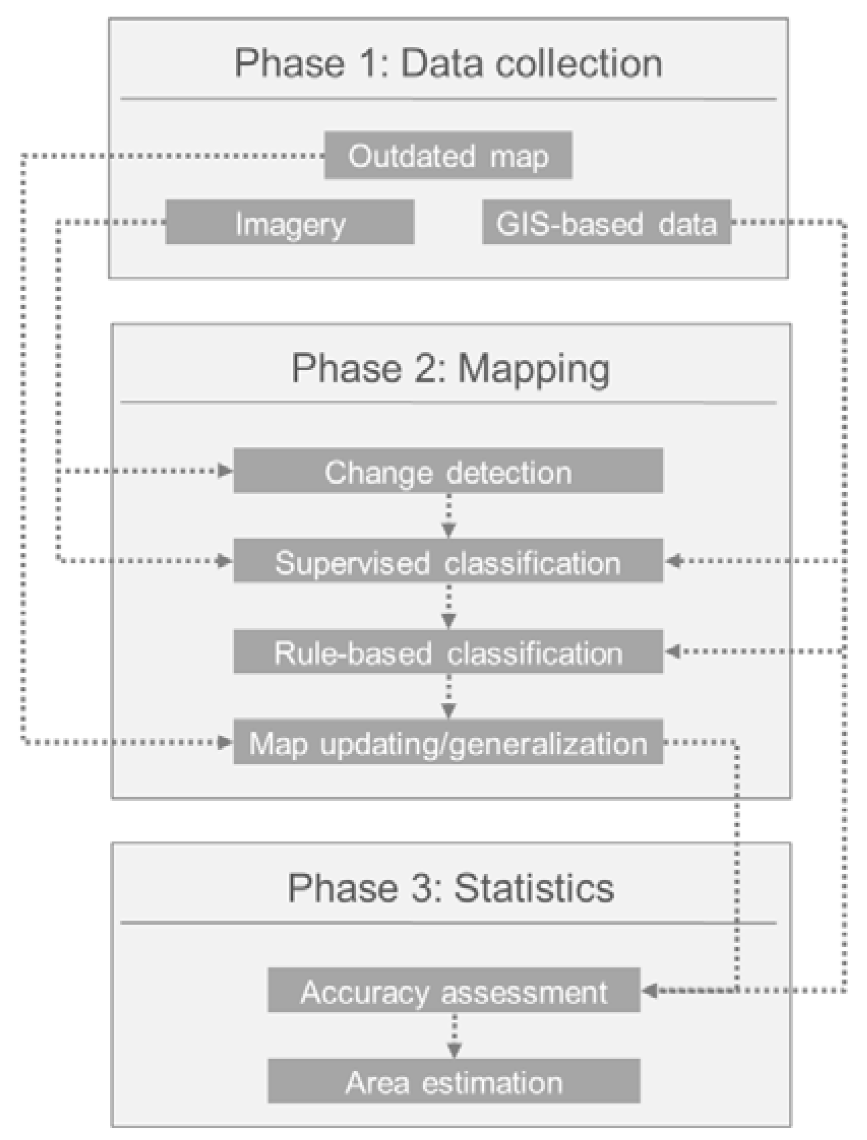
This paper presents and discusses the framework designed under the scope of LUCAS Grant 2015, centered on the production of land cover statistics for continental Portugal for a period of six years (2010–2015). The framework was designed to combine digital classification of remotely sensed data and available national geographical data sets and official statistics to estimate total areas of land cover classes. The methodology proposed in this paper can be applied elsewhere since it is grounded on the use of data under free access policy, following the EU Directive Infrastructure for Spatial Information in Europe (INSPIRE), at the same time that it is harmonized with data acquisition and dissemination procedures of the ESS. The results stress the potential of the general framework for continuous land cover statistics production, but difficulties and bottlenecks were found spanning mapping, accuracy assessment, and area estimation.

2. Study Area

Analyses focused on the continental territory of Portugal, which is located in the western extreme of the Iberian Peninsula, Europe (Figure 1). The area of continental Portugal is approximately 89,100 km2 and includes a diversity of natural conditions spanning generally a north–south gradient but also west–east due to the presence of the Atlantic Ocean in the west. Mediterranean and temperate climatic influences are found in the country and relatively hot and dry summers follow cold and wet winters. Mild weather conditions are typically found near the seaside, while rainy and dry weather characterize the north and south, respectively. Main settlements are located along the coastline, interwoven with low-density developed land. The Mediterranean bio-geographic region favors a great variety of landscapes displayed as a mosaic of forest, intensive agriculture, and wetlands associated with the major river mouths. Forests of eucalyptus targeted for production can be broadly found with native species of pines, scrublands, and fine-grained complex agricultural practices dominating large areas of the northern and hilly countryside; the typical Mediterranean silvopastoral system of oak stands concentrate in the southern peneplain. Both cases are punctuated by other land cover types, such as sprawling population centers and water reservoirs.
Land cover was defined based on the classification system of LUCAS, which has eight main categories: artificial land, cropland, woodland, shrubland, grassland, bareland, water, and wetland. These main categories are divided into 15 classes (Table 1) according to the hierarchical disaggregation of the classes of LUCAS and additional definitions of the Eurostat Annual Crop Statistics (ACS), Food and Agriculture Organization (FAO) of the United Nations, and INSPIRE Directive.

3. Materials and Methods

Statistics on land cover in continental Portugal were produced for 2010–2015 based on mapping. That is, a land cover map was produced for each year to support the estimation of land cover statistics. The year 2010 was selected as a base for statistics production. For this specific year, one main data source, the land use and land cover map (COS) (see Section 3.1.2), was used as the base map. Land cover was estimated from the map after accuracy assessment. In cases where no such map is available, one must be produced from scratch.
The general framework for map and statistics production for the following years included three main phases for updating the base map (Figure 2). First, data collection and analysis were performed under a free data acquisition policy and according to the project requirements, which combined a mixed methodology of applying remote sensing and auxiliary data to statistics. Second, a land cover map was produced for each of the years from 2011 to 2015. Third, the thematic accuracy of the maps was estimated and land cover statistics produced. The specific methods used are described in the following sections.

3.1. Data Collection

A comprehensive survey of data potentially meeting the requirement of the project and helpful for mapping land cover according to Table 1 was initially performed. In respect to remotely sensed data, Landsat imagery was considered convenient in terms of resolution (spatial, spectral, and temporal) and processing requirements. In terms of GIS-based data, numerous countrywide data sets were acquired and analyzed in respect to their suitability for the project, including their thematic information, temporal reference, and spatial representation. Details on the data sets finally used are given below.

3.1.1. Landsat Data

The remotely sensed data used were collected by three Landsat satellites (5, 7, and 8) during the summer and spring seasons of 2010–2015. Continental Portugal corresponds to eight Landsat images as defined in the Landsat’s Worldwide Reference System (Figure 1). The images were calibrated, converted to top-of-atmosphere reflectance, and atmospherically corrected. The processed images are delivered by the U.S. Geological Survey as surface reflectance [21,22].
The Landsat images were further processed according to the specifications described in the Landsat 4–7 Surface Reflectance Product Guide and Landsat 8 Surface Reflectance Product Guide before undertaking the analyses. Specifically, the pixels ranging between 0 and 10,000 were multiplied by the scale factor 0.0001; all the remaining pixels were reclassified as “no data” as they were outside the valid range of values. Pixels contaminated by clouds and cloud shadow were also reclassified as “no data.” After this initial processing step, the pixels represented surface reflectance raging between 0 and 1.
An additional processing analysis was needed to fill in the “no data” pixels with data, especially those of the Landsat images of 2012. These specific images were acquired by the Landsat 7 ETM+ sensor whose scan line corrector (SLC) failed permanently in 2003. In practical terms, since 2003, all images present striping effects in which the pixels have no data. In some other images, there were pixels with no data due to cloud cover and other issues. To overcome these problems, the pixels with no data were filled in with pixel values from other images of the same year. Table 2 summarizes the Landsat data used.
Six out of the eight Landsat path/rows were merged to define five regions here called tiles (Figure 1). Path/rows 204/31 and 204/32 were not merged, however, as the dates of the corresponding imagery were not compatible with other path/rows; tiles 3 and 4 correspond to these path/rows alone. Each tile was treated independently. Therefore, all the methods described in the following sections were performed five times per year (2011–2015). Reducing the initial eight path/rows to five tiles reduced some unnecessary routines and improved efficiency.

3.1.2. Auxiliary Data

The Land Use and Land Cover map (COS) is the official LCLU map of continental Portugal, produced through visual interpretation of orthophotomaps and auxiliary data for 1990, 1995, 2007, and 2010. COS of 2010 (COS2010) is a vectorial map with a minimum mapping unit (MMU) of one hectare and offers a detailed level of thematic and positional accuracy, harmonized with global and European policies related to geographic data quality and standards [23]. COS2010 was identified to provide improved thematic compliance with the project requirements and, thus, was selected as a base for statistics production. Therefore, the land cover nomenclature of COS, which is hierarchical and identifies 225 classes at the most detailed level, was converted to the nomenclature of Table 1, and an initial map was produced. That is, COS2010 was used to produce statistics for 2010 and then updated for the following years based on the remotely sensed data described above and the auxiliary data described below (Table 3).
Data were obtained from official national data sources to aid land cover mapping. Agriculture patches were identified on the Land Parcel Identification System (LPIS) of Instituto de Financiamento da Agricultura e Pescas (IFAP). LPIS is a countrywide spatial data set with information about the area, land cover, and physical limits of agricultural parcels, allowing farmers to apply for European subsidies and functions also as a means to control actions. LPIS is continually updated according to new funding requests and is based on aerial images. Quarries and wind farms were identified in the GIS-based data sets of Direção-Geral de Energia e Geologia (DGEG). These vectorial (polygons and points) data sets are continually updated. Wildfires were identified in the national mapping of burnt areas published by Instituto da Conservação da Natureza e das Florestas (ICNF). These vectorial (polygons) data set maps show burnt areas larger than five hectares at the end of each fire season based on visual interpretation of remotely sensed data (Landsat TM/ETM). While these auxiliary data were used for rule-based image classification, a digital elevation model at 30 m spatial resolution of the Shuttle Radar Topography Mission (SRTM) [24] was used as an aid for supervised image classification. Altitude and slope were useful for distinguishing some classes such as bare rock (consolidated bare surfaces), which tends to appear in mountainous regions.

3.2. Mapping

3.2.1. Change Detection

There are numerous methods to detect land cover change from remotely sensed data [25] but their implementation is not always straightforward. A relatively simple but effective approach for change detection is to compare remotely sensed data acquired on different dates. Some techniques based on this approach, often called differencing or layer arithmetic [18,25], calculate descriptive statistics for the difference of vegetation indices between two points in time. A threshold of the spectral difference is used to differentiate change from no-change pixels [26,27,28]. This technique was used here and land cover change was identified based on the Normalized Difference Vegetation Index (NDVI) [29] differencing.
The NDVI is expected to change from one year to the next due to many reasons (e.g., vegetation growth), but only substantial changes should reflect real land cover changes. Thus, the difference of NDVI between two years should in principle follow a normal distribution in which most of the differences observed are associated with natural variability of the surface reflectance and only few marked differences are caused by land cover change [26,27,28].
The pixels of the potential land cover change were identified if the magnitude of the difference between two successive years in terms of NDVI exceeded a threshold [26,27,28]. A threshold was defined for decreasing NDVI as two standard deviations away from the mean difference between the images compared. One standard deviation was defined as the threshold for the opposite case of increasing NDVI. The identified pixels could then be classified using the relevant Landsat images of the second year of the pair of years analyzed (see next sections). This strategy potentially detects land cover change if the pixels are allocated to a new land cover class, while the remaining pixels maintain the class of the previous year.

3.2.2. Supervised Image Classification

A training sample dedicated to each year was collected to perform per-pixel supervised image classifications. Each training pixel was allocated to a land cover class visually interpreted based on auxiliary data, such as Google street view and orthophotomaps of 2010, 2012, and 2015. The land cover classes used in training were, however, different from those desired in the maps (Table 1) as some of them correspond to a variety of spectral responses. For example, croplands include irrigated and non-irrigated crops, which have very distinct spectral properties. Moreover, some classes could be classified based on expert knowledge and/or auxiliary data (see Section 3.2.3). Therefore, spectral training classes rather than the final classes were used, namely, irrigated crops, non-irrigated crops, bare rock, bare soil, sand, forest, shrubland, grassland, and water. These classes may be adjusted as a function of the country to be mapped, data, etc.
The training samples preferably included pixels located in areas of variable NDVI, which are more representative of the areas of potential land cover change. However, the training samples excluded the pixels that by chance had no data originally and were filled in with pixel values from other images (Table 2). Nearly all classes were trained with 80 or more pixels per tile and per year, except 2012, for which 75 pixels on average were available per class due to the limited quantity of Landsat data for that year, as only the Landsat 7 satellite was operational and presenting striping effects (Table 2). In all cases, a minimum and a maximum of 50 and 100 pixels per class were accepted for training to ensure class representativeness and avoid very imbalanced samples. The total number of training pixels collected is presented in Table 4.
Three classifiers were used in the classification: (i) artificial neural network with no hidden layer (ANN) [30], (ii) random forest (RF) [31], and (iii) support vector machine (SVM) [32]. The ANN fits a multinomial linear regression that calculates the probability of a pixel belonging to a given class [30]. RF and SVM are non-parametric classifiers. The former is an ensemble of a tree-type classifier while the latter seeks to find the optimal separating hyperplane between classes based on the training cases that lie at the edge of the class distributions [33,34].
The settings of the non-parametric classifiers were defined through a resampling-based procedure to search for optimal tuning parameters [35]. Optimal settings were selected based on the mean overall accuracy across 10-fold cross validation, repeated twice. There was no need to define settings for the ANN as this is a special case of a neural network that uses neural net technology with no hidden layer to fit multinomial models [30].
The classifiers produced three classifications and a fourth and final classification was then generated through a voting process. Specifically, the final classification was determined by a majority vote of the three classifiers. For pixels in which all three classifiers disagreed, the classification of the SVM was adopted as, in general, the SVM was the most accurate classifier individually.

3.2.3. Rule-Based Image Classification

Several rule sets of the type if-then-else were defined based on expert knowledge to interpret the supervised image classifications with the help of auxiliary data. In some cases, thematic classes that were more detailed than required were identified, such as several agricultural classes and forest clear-cuts. Rules were defined to identify dynamic patches such as forest clear-cuts based on image classification. For example, a clear-cut was identified if a forest patch was classified as a bare surface in the following year. Other rules used the image classifications and auxiliary data together to address more challenging changes. For example, other built-up areas could be identified when removal of vegetation recorded in Landsat data and the wind farm locations provided by DGEG were spatially coincident. Overall, four main types of rules were defined and are summarized in Table 5. The detailed classification system and the rule set types used for mapping each class are shown in Table 6.
Note that although many classes were identified and a detailed nomenclature was possible, a conservative strategy was followed to reduce mapping false changes. That is, rules were defined so that only probable changes could be mapped (e.g., rules of type C). This ensured that errors included in the auxiliary data were not included in mapping.
This conservative strategy resulted in three classes (i.e., other land with tree cover, inland running water, and wetlands) not being mapped (Table 6). In general, these classes would require dedicated and complex methodologies (e.g., [36]) and/or data not available and, thus, satisfactory results were not guaranteed at this stage of the project. This means that new patches of these classes could not be identified from 2011 onwards. Therefore, the maps show only the patches of these classes that did not change since 2010. However, these classes are very stable over time and, thus, a negligible impact on the results was expected.

3.2.4. Map Updating and Generalization

The land cover changes identified between two consecutive years in the five tiles were merged to produce a single layer covering the entire country. Also, the detailed thematic classes were merged to the corresponding classes of Table 1. Converting changes from raster to vector format was needed since raster processing was the basis of image analysis; the maps that were to be produced needed to be vectorial according to the project requirements. The changes inevitably gave a grid-like appearance after conversion and, thus, were subjected to geometric smoothness. Then, the changes were superimposed on the map of the previous year to update it. This created small polygons, often called sliver polygons, which needed to be generalized to match the MMU of one hectare. Adopting a consistent MMU ensures comparability of the statistics produced for different years and, if needed, allows the use of remotely sensed data of various spatial resolutions. The sliver polygons were merged with the neighboring polygon with the longest shared border and the final land cover maps came out.

3.3. Statistics

3.3.1. Accuracy Assessment

A test data set was built through stratified random sampling. The strata corresponded to the spatial distribution of the 15 classes across continental Portugal as depicted in the map of 2010. One hundred points per class were collected, making 1500 points in total. The point is a valid spatial unit to assess the accuracy of polygonal maps [37]. Each point was assigned a primary and alternative, if needed, reference land cover class label for each of the years (i.e., 2010, 2011, etc.). The alternative label was needed when the point presented characteristics of more than one class, as often occurs in transitional land. To collect the reference data, very high-resolution orthophotomaps of 2010, 2012 and 2015, Google street view, and other auxiliary data sets were visually interpreted. The reference data collected for each year at each point were compared with each map to produce a confusion matrix. There was an agreement between the testing points and the maps if the latter matched the primary or alternative reference class label. Overall, users’ and producers’ accuracies were estimated according to [19].

3.3.2. Area Estimation

The area mapped of a class is close to the true area of cover if the map error is small. However, mapping error can be large and varies depending on the class. Thus, the area values obtained directly from a map may differ greatly from the true area. As stratified random sampling was used to assess the accuracy of mapping (previous section), it is possible to estimate the area of the land cover classes by adjusting the area for the mapping error. This was done using the unbiased estimator presented in [20] that includes the area of map omission error and leaves out the area of map commission error:
A ^ j = A t × i W i n i j n i +
where nij is the number of testing points of class j mapped as class i, ni+ is the total number of testing points of class i, Wi is the proportion of the total area mapped as class i, and At is the total area of the map.
Because area is estimated from a sample, uncertainty of each class j was quantified and reported by 95% confidence interval [20]:
A ^ j ± 1.96 × S ( A ^ j )
where S ( A ^ j ) is the standard error of the estimated area of class j and can be expressed as [20]:
S ( A ^ j ) = i W i 2 n i j n i + ( 1 n i j n i + ) n i + 1

4. Results

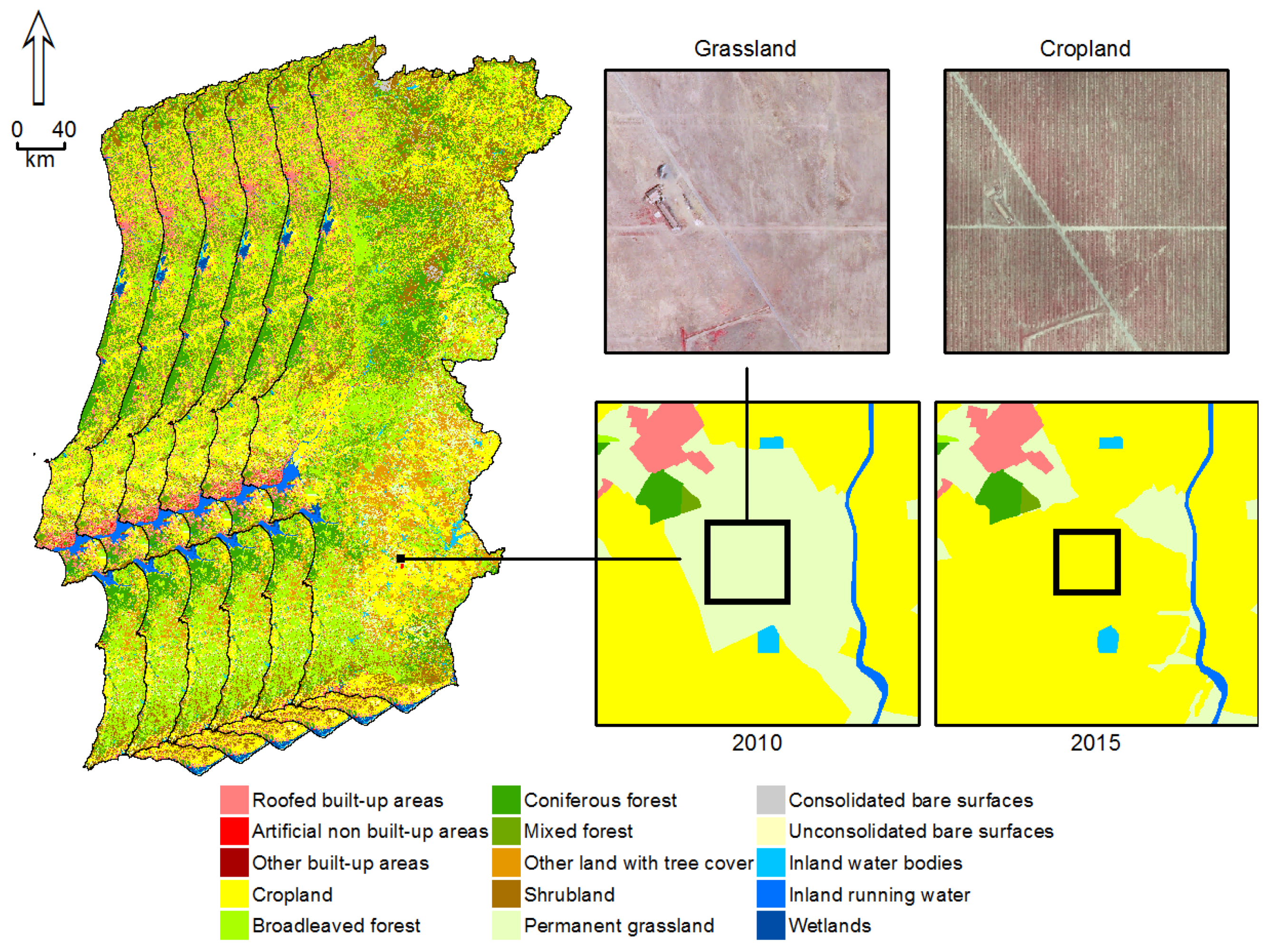
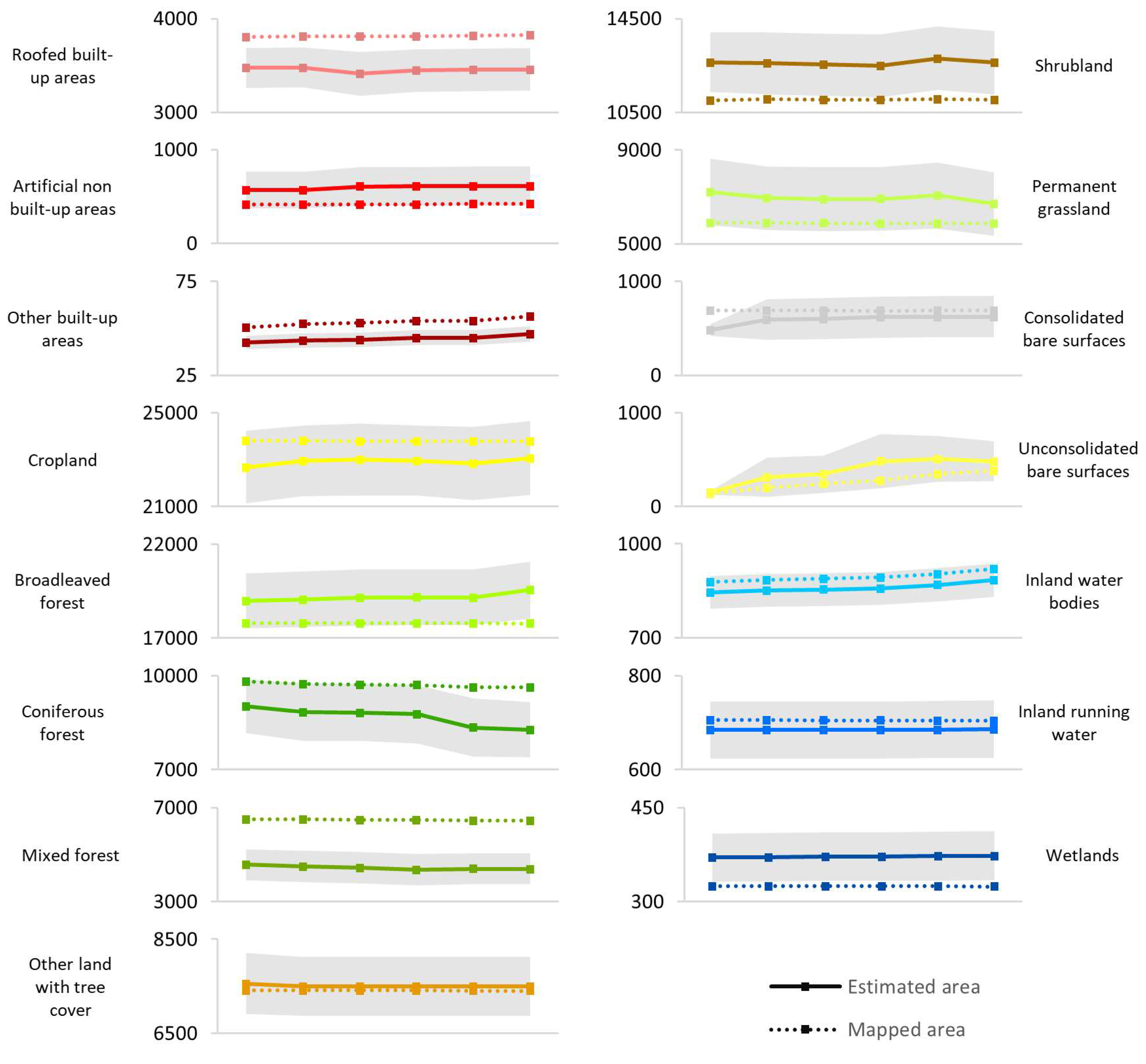
A land cover map was produced for 2010 (
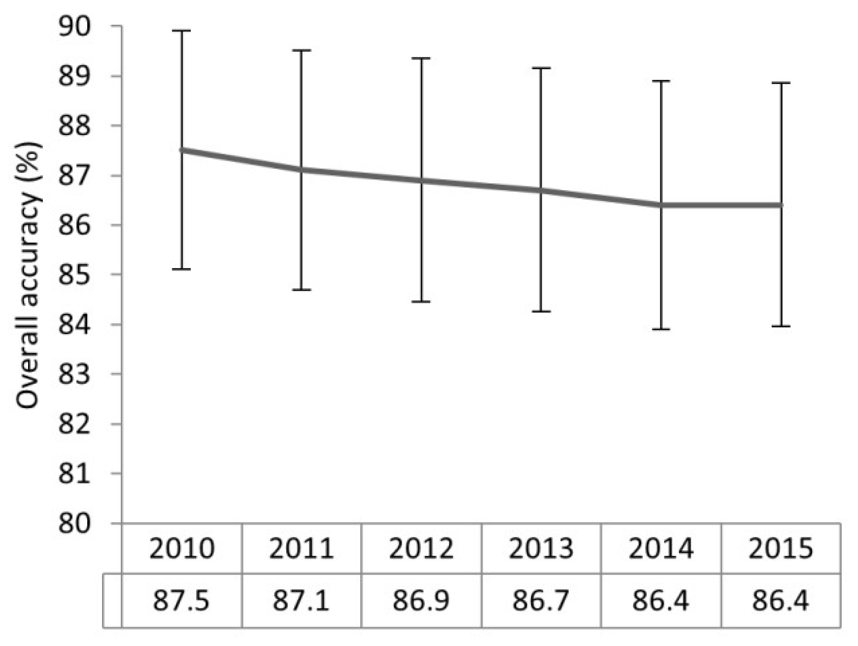
Figure 3) where cropland, woodland, shrubland, and grassland form approximately 92% of the mapped area. Artificial land, bareland, water, and wetlands are minority classes. The estimated overall accuracy of the 2010 map is 87.5%. This result is closely related to COS2010, as this official map was the basis for the map production.
Land cover is generally stable over time and, thus, similar maps were produced for the following years (Figure 3). Table 7 shows the area of each map that changed as compared to the precedent year’s map while Figure 3 shows an example of grassland converted to cropland. The estimated thematic accuracy of these maps is similar to that of 2010 but slightly smaller and follows a decreasing trend (Figure 4). The differences between the accuracy of the maps are not statistically significant.
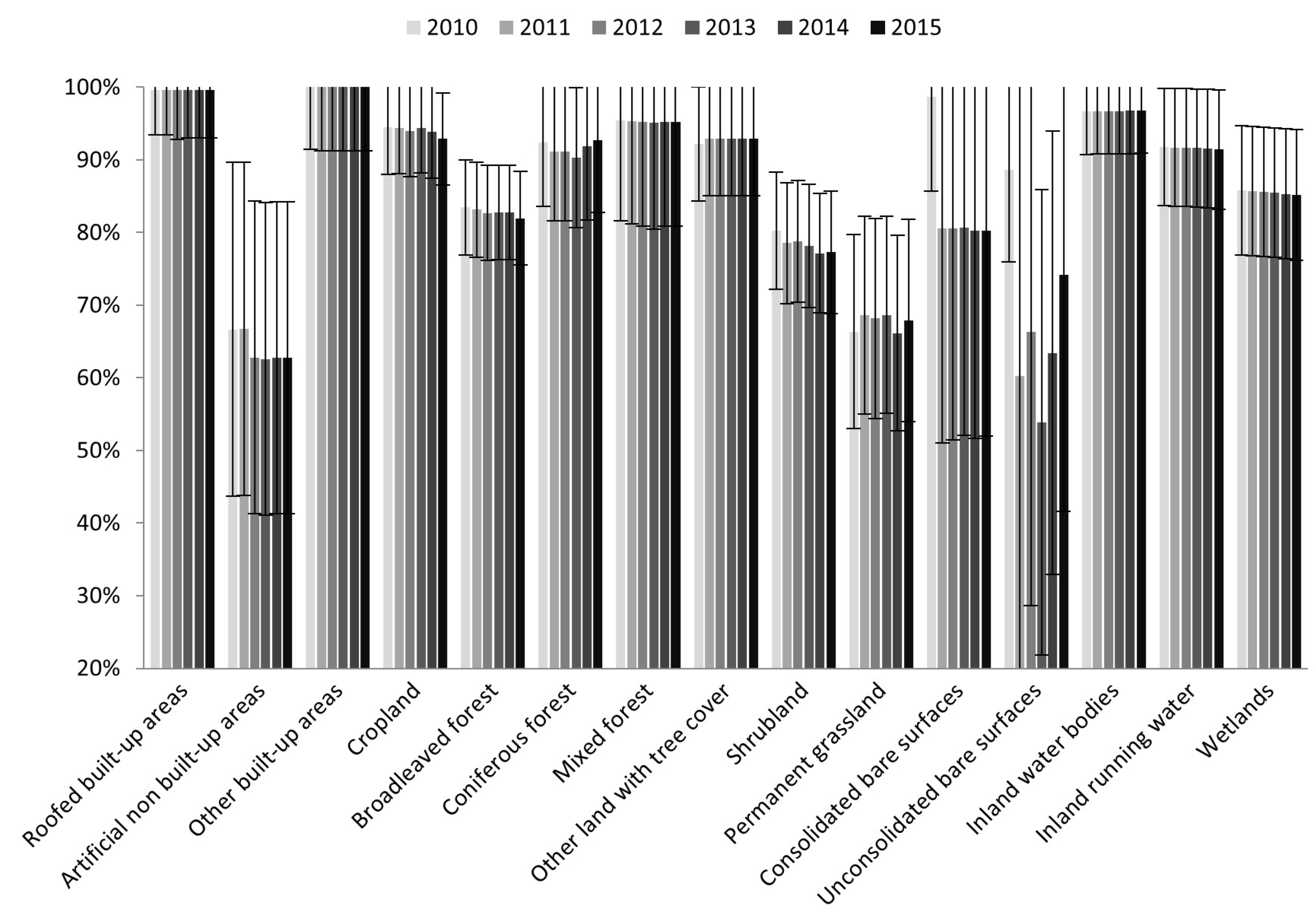
The overall accuracy of the maps depends on the accuracy of the classes mapped. Relatively more challenging classes present smaller user’s (Figure 5) or producer’s (Figure 6) accuracy, which expresses commission and omission errors, respectively. With regard to the former error type, mixed forest, consolidated bare surfaces, and permanent grassland are especially over-represented on the maps (relatively small user’s accuracy), and this error tended to increase over time, except for consolidated bare surfaces (Figure 5). On the other hand, artificial non-built-up areas, unconsolidated bare surfaces, and permanent grassland are under-represented (relatively small producer’s accuracy), with an unclear increasing or decreasing trend over time (Figure 6). Permanent grassland is particularly problematic as it accumulates considerable commission and omission map errors. In some cases, the difference between the accuracy of the classes is statistically significant, such as the user’s accuracy of artificial built-up areas and mixed forest (Figure 5). However, the differences between the maps for the accuracies of the same class over time are always statistically insignificant.
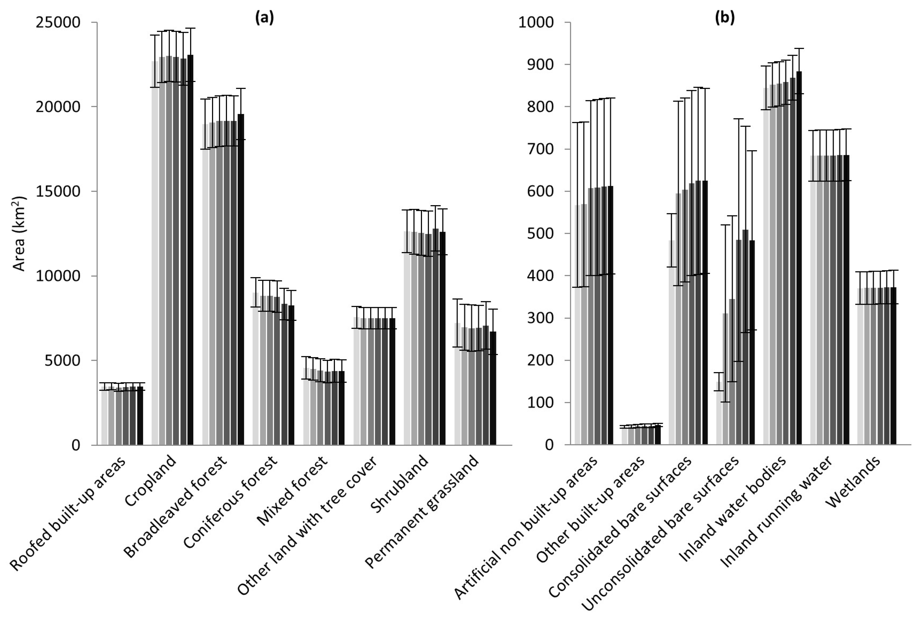
The mapped area of the land cover classes and the estimated error of the maps were used to estimate the actual area of each class in each year. The two most abundant classes (Figure 7a) are cropland (~23,000 km2) and broadleaved forest (~19,000 km2) and their abundance tended to increase during the period analyzed. Next, a group of six classes cover a relevant fraction of the territory: shrubland (~12,500 km2), coniferous forest (~9000 km2), other land with tree (~7500 km2), permanent grassland (~7200 km2), mixed forest (~4500 km2), and roofed built-up areas (~3500 km2). Differences between classes are statistically significant, except for coniferous forest, other land with trees, and permanent grassland, so the true order of their abundance may be swapped. The estimates suggest that the area of coniferous forests, mixed forests, and permanent grassland is in decline, while roofed built-up areas are expanding, although slightly. Then, a group of seven minority classes (Figure 7b) cover a total of ~2600 km2. Inland running water and other built-up areas are the most and least abundant minority classes (~850 km2 and ~42 km2), respectively. These classes are predominantly stable over time but unconsolidated bare surfaces increased substantially from 149 km2 in 2010 to 484 km2 in 2015. To note in most cases, the evolution of the classes’ areas over time indicates differences in estimations, which are not statistically significant. Despite the interest that drivers for landscape change may be raised by these results, they are out of the scope of this paper.

5. Discussion

5.1. Mapping

A total of five land cover maps were produced by successively updating an initial map. The differences between the maps were expected to be relatively small as previous studies show an average land change rate of 1.1% for the region every year between 1995 and 2007 and 0.3% between 2007 and 2010 [38]. These statistics were produced using a nomenclature of nine classes. Thus, slightly larger change statistics were deemed possible for the period 2010–2015 as more classes were used. However, the differences between the maps ranged from 0.12% to 0.25% of the mapped area.
This result is possibly related to the slowdown of land cover change in Portugal observed between 1995 and 2010, which may have continued through 2010–2015. However, while this argument is somewhat speculative, there are objective reasons to believe that some land cover change went unnoticed. Overall accuracy followed a decreasing and undesirable trend (Figure 4). This suggests that the methods used for map updating were less effective than those used to produce the first map (visual interpretation of very high-resolution orthophotomaps and auxiliary data). Specifically, the increased mapped area of some classes related to larger mapping error (see Section 5.2) may have acted to decrease the overall accuracy.
A practical method was used for change detection but it is largely dependent on the thresholds selected to discriminate change from no-change [18,25]. While this issue is minor when land cover change corresponds to abrupt NDVI changes (e.g., severe vegetation removal), some concerns arise when the NDVI changes smoothly. The latter may correspond, for example, to a new forest patch with small growth rates. An improvement to the method could be to allow for flexibility and therefore vary the thresholds of change over time and space to adapt to temporary and local conditions. Alternative methods should also be tested [25].
Change detection may also have suffered from the remotely sensed time series that was used. A time series of a few years may be too short to detect some regeneration and succession. This may be relevant especially in the first years of the series, such as 2011, as data before 2010 were not available. Therefore, a longer time series is recommended, which may include data from diverse sensors such as that collected by the Sentinel constellation [39,40].
Another cause for missing land cover changes is the conservative mapping strategy adopted (e.g., rule set C). Such a strategy promotes robustness of mapping but is unable to cope with possible incongruity between the satellite and auxiliary data. This issue was common in terms of temporal reference as the satellite data have specific acquisition dates, while the auxiliary data sets often refer to vague dates. Two ways may be followed to address this issue. First, the rule-based classification step may allow for flexibility on the temporal match regarded as acceptable between the satellite and auxiliary data. For example, mapping of a specific year may include contributions from the auxiliary data available for a time window around the year of interest. A larger land cover change will certainly be detected and mapped as a result but certainly at the expense of some inaccuracy about the year of change. However, the benefits of mapping land change imprecisely greatly outweigh the loss of not mapping change at all. The second measure for coping with incongruity is to liaise with data producers. Simple adjustments on data production may be needed, such as including a specific date related to land change while updating GIS-based records.
Map updating and generalization adopted a simple approach of merging polygons with the longest shared border. This makes generalization biased towards large polygons, which tend to define the longest shared border of small polygons. Also, the 30 m raster format classifications were converted to vector format, which may distort or produce undesirable geometries. In theory, this issue may have a small impact on the results as errors caused by geometry distortions may compensate for each other and, hence, preserve the relative abundance of the classes. However, landscape structure may be fragmented and some classes may tend to cover smaller patches than other classes, which can affect per-class classification accuracy; smaller patches are challenging to classify [41] and are found in some regions of the country, such as suburban areas of small and mixed agricultural fields, forest patches, built-up areas, etc.
Other issues may have affected the results negatively, such as insufficient correction for clouds and atmospheric effects. This is particularly relevant when alternative images were used to fill in pixels with no data (Table 2). This correction is problematic when the vegetation phenology or some other change occurs between data acquisitions, thereby causing the detection of false land cover changes. This issue had a minor impact in practice. Many false changes were masked by the MMU or allocated to the same class as mapped in the previous year, thereby neutralizing false change.
Some other issues are expected to have an impact on the result but are not necessarily negative. For example, ensemble classification possibly afforded larger accuracy than the traditional practice of using a single classifier and further exploration of this approach may offer further accuracy. The MMU of one hectare was adopted as the vector map of 2010 used this initially. Different values for the MMU could have been defined with little impact on map accuracy and statistics.

5.2. Statistics

The quality of the land cover statistics produced from mapping inherits the limitations discussed above. However, good practices for classification accuracy assessment and area estimation can minimize the issue. Random sampling enables the estimation of commission and omission errors, which can be used to compensate for map error while producing the statistics. Thus, the statistics indicate that the area of broadleaved forests followed an increasing trend from ~19,000 km2 to ~20,500 km2 (Figure 8) whereas the mapped area of this class remained stable across all maps (~17,800 km2). The differences between the statistics over time are not statistically significant at the 95% confidence level as the confidence intervals overlap (Figure 7). However, an increasing area of broadleaved forest was expected according to historical observations since eucalyptus plantations began to increase mainly due to paper manufacturing.
The statistics produced show that in some cases compensation for map error was insufficient. For example, a relatively strong increase in the area of unconsolidated bare surfaces was estimated (Figure 7) as the mapped area of this class increased (Figure 8). However, a part of the mapped area of the class is forest. The confusion between the classes stems from change involving the removal of vegetation, such as shrubs, so that tree plantations could follow. Such areas were classified as bare land while the vegetation was removed; however, such classification should be temporary and remain only until the plantation has grown. However, as noted above, vegetation growth is difficult to detect, as the NDVI tends to increase smoothly. Therefore, new forest patches often remain classified as bare land.
Limited compensation for map error of unconsolidated bare surfaces may be related to two factors. First, the extent of relatively rare classes, as in the case of unconsolidated bare surfaces, is typically overestimated [42]. Next, area estimation based on accuracy assessment typically assumes that the testing data contains no error. This may be untrue despite the efforts to produce a gold standard as it is common in the remote sensing community [43]. Errors embedded in testing data impacts area estimations and amplifies the tendency for overestimating rare classes [42].
Then, the size of the test data set may have been small. Note that a relatively strong increase in the area of unconsolidated bare surfaces was mapped and estimated as discussed above but the producer’s accuracies (Figure 6) suggest that this class is under-represented. This may be caused by a spatially clustered distribution of map error that is difficult to detect if the test data set is small and hence spatially sparse. A larger test data set would have detected more easily the commission errors of rare classes proportionally to the amount of error. The precision of all estimates would have increased as well.

5.3. Transfer and Improvement

The framework proposed was illustrated for Portugal and modifications are needed for its operational application. The success of mapping and production of harmonized statistics largely depends on the data used and land cover patterns, which typically vary from country to country. Thus, for example, the rule-based image classification step will have to be revised and rewritten, not only to adapt to different contexts but also to integrate a variety of data sets. These, however, are increasingly harmonized across Europe, for example, due to the INSPIRE Directive. Full and exhaustive exploration of auxiliary data should be performed, including those commonly available for the countries and not used here, such as cadaster and roadmaps. Furthermore, data from private sources can be incorporated into the methodology after ensuring they meet acceptable quality and technical standards. Making use of auxiliary data is perhaps the aspect of the methodology most dependent on the context of the application.
It is also important that action is taken to improve map accuracy within each individual case. For example, advanced training methods with a focus on operational use [44,45,46,47,48] can be explored to improve the supervised image classification stage. Moving from pixel-based to object-based image analysis (OBIA) may also be advantageous, especially if a vector land cover map is desired. OBIA enables the geometry of the auxiliary GIS-based data to be incorporated directly into the image classification with a reduced need of generalization as raster to vector conversion is avoided. If, however, pixel-based image analysis is performed, map generalization should use semantic rules rather than geometric rules to decide polygon merging. The general framework proposed here can accommodate both pixel- and object-based image analyses.
Mapping is a fundamental component of the framework but land cover statistics production is critical. Land cover mapping will always experience error and statistical methods should account for it. Future research should address three main issues in this regard. First, the error embedded in the reference data and the uneven abundance of land cover types negatively impacts the area estimation. The influence of these issues is known in general [42] but the magnitude of the impact is specific to each case and unknown. Second, land cover statistics must commonly be produced for specific regions of a country, such as the NUTS in Europe, but the traditional accuracy assessment protocols are implemented to assess entire maps. Thus, the statistics produced are valid for the entire extent of the maps only, which commonly is the total extent of a country such as Portugal in this study. This is because sound accuracy assessment typically builds on a random testing sample and confusion matrix, which inevitably demand much effort and time [19]. Thus, replicating accuracy assessment for multiple regions, such as NUTS individually, is unfeasible. In practice, geographical fluctuations of the map accuracy are unknown as the confusion matrix produced summarizes the entire maps. Third, often a testing data set is reused to assess the thematic accuracy of several maps for similar practical reasons. This is problematic when stratified sampling is used and based on strata defined by one of the maps, which changes every time it is updated. As such, the strata defined by the updated maps are no longer coincident with the strata used in sampling. In such cases, the estimators proposed by [49] can be used as they account for the difference between the map and sampling strata. However, larger standard errors are expected [49], which may be undesirable.

6. Conclusions

A general framework for frequent land cover mapping was explored with the ultimate goal of producing harmonized land cover statistics across Europe. The methodology proposed aims to be repeatable and transferable, which requires adjustments to some of the methods that populated the workflow used in the Portuguese case study. The adjustments should address the limitations identified here and the particularities of each country, such as data availability and land cover patterns.
The first phase of the framework is the ground foundation of the whole methodology—data collection plays a crucial role in gathering relevant and official data sets. Despite its relevance, data collection was not discussed in this paper. Data set coherence and harmonization depend largely on the reality of each country. The final data sets used would benefit from a partnership selection between national authorities and Eurostat to ensure harmonized and quality-assured statistics. Land cover mapping, the second phase of the general framework, is formed by change detection, two-stage image classification, and map updating and generalization. An effective change detection method should be used, which can be adopted by different countries, as only satellite data are needed. Likewise, map updating and generalization are not dependent on national contexts and the same method can be widely adopted. Therefore, the variety of natural conditions and human activities of each country should be considered mainly to design the supervised and rule-based image classifications. This requires the definition of tailored spectral classes for supervised image classification able to provide meaningful information to the second classification, which should be adapted to interpret the preliminary classification and national GIS-based data sets. The combination of supervised and rule-based classifications is perhaps a singular aspect of the framework as it enables numerous opportunities for larger mapping accuracy and transference to other countries. An estimation of the area from the maps, the last framework’s phase, can take advantage of the accuracy assessment information to compensate for the estimated map errors; however, some challenges remain, such as removing bias related to the uneven abundance of the land cover classes and producing statistics valid for sub-national regions. The development of alternative accuracy assessment approaches with clear advantages for operational use [50,51] is recommended.

Acknowledgments

The methodology presented in this paper derives from the development of a national methodology to produce Land Use and Land Cover statistics on a regular basis, under the scope of LUCAS Grant 2015, supported by Eurostat under contract number 08441.2015.002-2015.724. Further research and outputs reported in this paper were carried out and supported by the NOVA Information Management School (NOVA IMS) Research and Development Center (MagIC).

Author Contributions

H.C. and M.C. conceived and designed the experiments; H.C. performed the experiments; all authors analyzed the data and results; H.C. led the writing with inputs from all authors.

Conflicts of Interest

The authors declare no conflict of interest. The founding sponsors had no role in the design of the study; in the collection, analyses, or interpretation of data; in the writing of the manuscript, and in the decision to publish the results.

References

  1. Pielke, R.A. Land use and climate change. Science 2005, 310, 1625–1626. [Google Scholar] [CrossRef] [PubMed]
  2. Luyssaert, S.; Jammet, M.; Stoy, P.C.; Estel, S.; Pongratz, J.; Ceschia, E.; Churkina, G.; Don, A.; Erb, K.; Ferlicoq, M.; et al. Land management and land-cover change have impacts of similar magnitude on surface temperature. Nat. Clim. Chang. 2014, 4, 389–393. [Google Scholar] [CrossRef]
  3. UNFCC. Adoption of the Paris Agreement; Report No. FCCC/CP/2015/L.9/Rev.1; United Nations Framework Convention on Climate Change: New York, NY, USA, 2015. [Google Scholar]
  4. EUROSTAT. The EU’s Land Use and Land Cover Survey; 2017 Edition; Compact Guide; EUROSTAT: Luxembourg, 2017. [Google Scholar]
  5. Grekousis, G.; Mountrakis, G.; Kavouras, M. An overview of 21 global and 43 regional land-cover mapping products. Int. J. Remote Sens. 2015, 1161, 1–27. [Google Scholar] [CrossRef]
  6. Congalton, R.; Gu, J.; Yadav, K.; Thenkabail, P.; Ozdogan, M. Global Land Cover Mapping: A Review and Uncertainty Analysis. Remote Sens. 2014, 6, 12070–12093. [Google Scholar] [CrossRef]
  7. Büttner, G. CORINE Land Cover and Land Cover Change Products. In Land Use and Land Cover Mapping in Europe: Practices & Trends; Manakos, I., Braun, M., Eds.; Springer: Dordrecht, The Netherlands, 2014; pp. 55–74. [Google Scholar]
  8. Latifovic, R.; Homer, C.; Ressl, R.; Pouliut, D.; Hossain, S.N.; Colditz, R.R.; Olthof, I.; Giri, C.; Victoria, A. North American Land Change Monitoring System. In Remote Sensing of Land Use and Land Cover: Principles and Applications; Giri, C.P., Ed.; CRC Press: Boca Raton, FL, USA, 2014; pp. 303–324. [Google Scholar]
  9. Latifovic, R.; Pouliot, D.; Olthof, I. Circa 2010 Land Cover of Canada: Local Optimization Methodology and Product Development. Remote Sens. 2017, 9, 1098. [Google Scholar] [CrossRef]
  10. Colditz, R.R.; Pouliot, D.; Llamas, R.M.; Homer, C.G.; Latifovic, R.; Ressl, R.; Meneses Tovar, C.; Victoria Hernández, A.; Richardson, K. North American-wide land cover change detection between 2005 and 2010 with 250 m MODIS data. Photogramm. Eng. Remote Sens. 2014, 80, 918–924. [Google Scholar]
  11. Pax-Lenney, M.; Woodcock, E.C.; Macomber, A.S.; Gopal, S.; Song, C. Forest mapping with a generalized classifer and Landsat TM data. Remote Sens. Environ. 2001, 77, 241–250. [Google Scholar] [CrossRef]
  12. Comber, A.J.; Law, A.N.R.; Lishman, J.R. A comparison of Bayes’, Dempster-Shafer and Endorsement theories for managing knowledge uncertainty in the context of land cover monitoring. Comput. Environ. Urban Syst. 2004, 28, 311–327. [Google Scholar] [CrossRef]
  13. Latifovic, R.; Pouliot, D. Multitemporal land cover mapping for Canada: Methodology and products. Can. J. Remote Sens. 2005, 31, 347–363. [Google Scholar] [CrossRef]
  14. Fraser, R.H.; Olthof, I.; Pouliot, D. Monitoring land cover change and ecological integrity in Canada’s national parks. Remote Sens. Environ. 2009, 113, 1397–1409. [Google Scholar] [CrossRef]
  15. Xian, G.; Homer, C. Updating the 2001 National Land Cover Database Impervious Surface Products to 2006 using Landsat Imagery Change Detection Methods. Remote Sens. Environ. 2010, 114, 1676–1686. [Google Scholar] [CrossRef]
  16. Pouliot, D.; Latifovic, R.; Olthof, I.; Fraser, R. Supervised Classification Approaches for the Development of Land-Cover Time Series. In Remote Sensing of Land Use and Land Cover; Giri, C., Ed.; CRC Press: Boca Raton, FL, USA, 2012; pp. 177–190. [Google Scholar]
  17. Pouliot, D.; Latifovic, R.; Zabcic, N.; Guindon, L.; Olthof, I. Development and assessment of a 250 m spatial resolution MODIS annual land cover time series (2000–2011) for the forest region of Canada derived from change-based updating. Remote Sens. Environ. 2013, 140, 731–743. [Google Scholar] [CrossRef]
  18. Zhu, Z. Change detection using landsat time series: A review of frequencies, preprocessing, algorithms, and applications. ISPRS J. Photogramm. Remote Sens. 2017, 130, 370–384. [Google Scholar] [CrossRef]
  19. Olofsson, P.; Foody, G.M.; Herold, M.; Stehman, S.V.; Woodcock, C.E.; Wulder, M.A. Good practices for estimating area and assessing accuracy of land change. Remote Sens. Environ. 2014, 148, 42–57. [Google Scholar] [CrossRef]
  20. Olofsson, P.; Foody, G.M.; Stehman, S.V.; Woodcock, C.E. Making better use of accuracy data in land change studies: Estimating accuracy and area and quantifying uncertainty using stratified estimation. Remote Sens. Environ. 2013, 129, 122–131. [Google Scholar] [CrossRef]
  21. Masek, J.G.; Vermote, E.F.; Saleous, N.E.; Wolfe, R.; Hall, F.G.; Huemmrich, K.F.; Gao, F.; Kutler, J.; Lim, T.-K. A Landsat surface reflectance dataset for North America, 1990-2000. IEEE Geosci. Remote Sens. Lett. 2006, 3, 68–72. [Google Scholar] [CrossRef]
  22. Vermote, E.; Justice, C.; Claverie, M.; Franch, B. Preliminary analysis of the performance of the Landsat 8/OLI land surface reflectance product. Remote Sens. Environ. 2016, 185, 46–56. [Google Scholar] [CrossRef]
  23. DGT. Especificações técnicas da Carta de uso e ocupação do solo de Portugal Continental para 1995, 2007 e 2010; Direção-Geral do Território, Relatório técnico: Lisbon, Portugal, 2016. [Google Scholar]
  24. Farr, T.; Rosen, P.; Caro, E.; Crippen, R.; Duren, R.; Hensley, S.; Kobrick, M.; Paller, M.; Rodriguez, E.; Roth, L.; et al. The shuttle radar topography mission. Rev. Geophys. 2007, 45, 1–33. [Google Scholar] [CrossRef]
  25. Tewkesbury, A.P.; Comber, A.J.; Tate, N.J.; Lamb, A.; Fisher, P.F. A critical synthesis of remotely sensed optical image change detection techniques. Remote Sens. Environ. 2015, 160, 1–14. [Google Scholar] [CrossRef]
  26. Lu, D.; Mausel, P.; Brondízio, E.; Moran, E.F. Change detection techniques. Int. J. Remote Sens. 2004, 25, 2365–2401. [Google Scholar] [CrossRef]
  27. Pu, R.; Gong, P.; Tian, Y.; Miao, X.; Carruthers, R.I.; Anderson, G.L. Using classification and NDVI differencing methods for monitoring sparse vegetation coverage: A case study of saltcedar in Nevada, USA. Int. J. Remote Sens. 2008, 29, 3987–4011. [Google Scholar] [CrossRef]
  28. Jin, S.; Yang, L.; Danielson, P.; Homer, C.; Fry, J.; Xian, G. A comprehensive change detection method for updating the National Land Cover Database to circa 2011. Remote Sens. Environ. 2013, 132, 159–175. [Google Scholar] [CrossRef]
  29. Tucker, C.J. Red and photographic infrared linear combinations for monitoring vegetation. Remote Sens. Environ. 1979, 8, 127–150. [Google Scholar] [CrossRef]
  30. Venables, W.N.; Ripley, B.D. Modern Applied Statistics with S; Springer: New York, NY, USA, 2002; ISBN 978-0-387-21706-2. [Google Scholar]
  31. Liaw, A.; Wiener, M. Classification and Regression by randomForest. R News 2002, 2, 18–22. [Google Scholar] [CrossRef]
  32. Meyer, D.; Dimitriadou, E.; Hornik, K.; Weingessel, A.; Leisch, F. e1071: Misc Functions of the Department of Statistics, Probability Theory Group (Formerly: E1071), TU Wien. R package version 1.6-8. 2017. Available online: https://CRAN.R-project.org/package=e1071 (accessed on 16 February 2018).
  33. Foody, G.M.; Mathur, A. A relative evaluation of multiclass image classification by support vector machines. IEEE Trans. Geosci. Remote Sens. 2004, 42, 1335–1343. [Google Scholar] [CrossRef]
  34. Gislason, P.; Benediktsson, J.; Sveinsson, J. Random Forests for land cover classification. Pattern Recognit. Lett. 2006, 27, 294–300. [Google Scholar] [CrossRef]
  35. Kuhn, M. caret: Classification and Regression Training. R package version 6.0-71. 2016. Available online: https://CRAN.R-project.org/package=caret (accessed on 16 February 2018).
  36. Godinho, S.; Guiomar, N.; Gil, A. Using a stochastic gradient boosting algorithm to analyse the effectiveness of Landsat 8 data for montado land cover mapping: Application in southern Portugal. Int. J. Appl. Earth Obs. Geoinf. 2016, 49, 151–162. [Google Scholar] [CrossRef]
  37. Stehman, S.V.; Wickham, J.D. Pixels, blocks of pixels, and polygons: Choosing a spatial unit for thematic accuracy assessment. Remote Sens. Environ. 2011, 115, 3044–3055. [Google Scholar] [CrossRef]
  38. Caetano, M.; Igreja, C.; Marcelino, F.; Costa, H. Estatísticas e dinâmicas territoriais multiescala de Portugal Continental 1995-2007-2010 com base na Carta de Uso e Ocupação do Solo (COS); Direção-Geral do Território, Relatório técnico: Lisbon, Portugal, 2017. [Google Scholar]
  39. Clerici, N.; Valbuena Calderón, C.A.; Posada, J.M. Fusion of Sentinel-1A and Sentinel-2A data for land cover mapping: A case study in the lower Magdalena region, Colombia. J. Maps 2017, 13, 718–726. [Google Scholar] [CrossRef]
  40. Wang, Q.; Blackburn, G.A.; Onojeghuo, A.O.; Dash, J.; Zhou, L.; Zhang, Y.; Atkinson, P.M. Fusion of Landsat 8 OLI and Sentinel-2 MSI Data. IEEE Trans. Geosci. Remote Sens. 2017, 55, 3885–3899. [Google Scholar] [CrossRef]
  41. Castilla, G.; Hernando, A.; Zhang, C.; McDermid, G.J. The impact of object size on the thematic accuracy of landcover maps. Int. J. Remote Sens. 2014, 35, 1029–1037. [Google Scholar] [CrossRef]
  42. Foody, G.M. Ground reference data error and the mis-estimation of the area of land cover change as a function of its abundance. Remote Sens. Lett. 2013, 4, 783–792. [Google Scholar] [CrossRef]
  43. Foody, G.M. Harshness in image classification accuracy assessment. Int. J. Remote Sens. 2008, 29, 3137–3158. [Google Scholar] [CrossRef]
  44. Kim, Y.; Park, N.-W.; Lee, K.-D. Self-Learning Based Land-Cover Classification Using Sequential Class Patterns from Past Land-Cover Maps. Remote Sens. 2017, 9, 921. [Google Scholar] [CrossRef]
  45. Dannenberg, P.M.; Hakkenberg, R.C.; Song, C. Consistent Classification of Landsat Time Series with an Improved Automatic Adaptive Signature Generalization Algorithm. Remote Sens. 2016, 8, 691. [Google Scholar] [CrossRef]
  46. Zhu, Z.; Gallant, A.L.; Woodcock, C.E.; Pengra, B.; Olofsson, P.; Loveland, T.R.; Jin, S.; Dahal, D.; Yang, L.; Auch, R.F. Optimizing selection of training and auxiliary data for operational land cover classification for the LCMAP initiative. ISPRS J. Photogramm. Remote Sens. 2016, 122, 206–221. [Google Scholar] [CrossRef]
  47. Silva, J.; Bacao, F.; Dieng, M.; Foody, G.M.; Caetano, M. Improving specific class mapping from remotely sensed data by cost-sensitive learning. Int. J. Remote Sens. 2017, 38, 3294–3316. [Google Scholar] [CrossRef]
  48. Demir, B.; Bovolo, F.; Bruzzone, L. Updating Land-Cover Maps by Classification of Image Time Series: A Novel Change-Detection-Driven Transfer Learning Approach. IEEE Trans. Geosci. Remote Sens. 2013, 51, 300–312. [Google Scholar] [CrossRef]
  49. Stehman, S.V. Estimating area and map accuracy for stratified random sampling when the strata are different from the map classes. Int. J. Remote Sens. 2014, 35, 37–41. [Google Scholar] [CrossRef]
  50. Foody, G.M. Latent class modeling for site- and non-site-specific classification accuracy assessment without ground data. IEEE Trans. Geosci. Remote Sens. 2012, 50, 2827–2838. [Google Scholar] [CrossRef]
  51. Fonte, C.C.; Martinho, N. Assessing the applicability of OpenStreetMap data to assist the validation of land use/land cover maps. Int. J. Geogr. Inf. Sci. 2017, 31, 2382–2400. [Google Scholar] [CrossRef]
Figure 1. Continental Portugal and corresponding Landsat path/rows. Colors indicate merged path/rows to define five tiles used in image processing and classification.
Ijgi 07 00157 g001
Figure 2. Framework overview.
Ijgi 07 00157 g002
Figure 3. Land cover maps and an example of land cover change (grassland to cropland).
Ijgi 07 00157 g003
Figure 4. Estimated overall accuracy of the maps with a 95% confidence interval.
Ijgi 07 00157 g004
Figure 5. Estimated user’s accuracy of the maps with a 95% confidence interval.
Ijgi 07 00157 g005
Figure 6. Estimated producer’s accuracy of the maps with a 95% confidence interval.
Ijgi 07 00157 g006
Figure 7. Estimated area of the land cover classes with a 95% confidence interval. Most and least abundant classes are shown separately in (a,b) to improve readability.
Ijgi 07 00157 g007
Figure 8. Difference between mapped and estimated area of the land cover classes. All plots present time (from 2010 to 2015) in the x-axis and area (km2) in the y-axis. Shaded areas represent 95% confidence intervals.
Ijgi 07 00157 g008
Table 1. Land cover classification system (main LUCAS categories are shown in capitals for guidance).
ClassDescriptionReference
A ARTIFICIAL LAND
Roofed built-up areasRoofed constructions that can be entered by persons.LUCAS
Artificial non-built-up areasNon-built-up areas characterized by an artificial and/or impervious cover of hard artificial material, concrete, gravel.LUCAS
Other built-up areasOther artificial areas (such as power plants and water sewage plants).LUCAS
B CROPLAND
CroplandAreas where crops are planted and cultivated.LUCAS
C WOODLAND
Broadleaved forestWoodlands composed of more than 75% of broadleaved species.FAO/LUCAS
Coniferous forestWoodlands composed of more than 75% of coniferous species.FAO/LUCAS
Mixed forestWoodlands composed of broadleaved and coniferous trees comprising both >25% of the tree canopy.FAO/LUCAS
Other land with tree coverAgricultural or urban land with 10% or more tree cover able to reach a height of 5 meters at maturity.FAO/LUCAS
D SHRULAND
ShrublandAreas dominated (at least 10% of the surface) by shrubs and low woody plants normally not able to reach more than 5 m of height. It may include sparsely occurring trees with a canopy below 10%.LUCAS
E GRASSLAND
GrasslandSown or self-seeded grassland, grass-like plants, and forbs without trees and shrubland and that are not included in the crop rotation on the holding.LUCAS/ACS
F BARE LAND AND LICHENS/MOSS
Consolidated bare surfacesConsolidated bare surfaces and organic and chemical deposits.INSPIRE
Unconsolidated bare surfacesUnconsolidated bare surfaces, organic and chemical deposits, and intertidal flats assigned to inland areas.INSPIRE
G WATER AREAS
Inland water bodiesInland areas of still standing surface water.LUCAS
Inland running waterInland channels of running water.LUCAS
H WETLANDS
WetlandsAreas that fall between land and water and wet for long enough periods that the plants and animals living in or near them are adapted to, and often dependent on, wet conditions for at least part of their life cycle.LUCAS
Table 2. Landsat data.
YearPathRowSpringSummer
Date [Landsat]Additional Date(s) [Landsat]Date [Landsat]Additional Date(s) [Landsat]
20102043119-May [7] 30-July [5]
3225-April [5] 30-July [5]
3325-April [5] 30-July [5]
3425-April [5] 30-July [5]8-September [7]
2033120-May [5] 21-June [5]
3220-May [5] 21-June [5]
3320-May [5] 21-June [5]
344-May [5] 21-June [5]
20112043128-April [5]4-April [7]; 19-March [7]1-July [5]18-August [5]
3228-April [5]14-May [5]; 19-March [7]25-July [7]10-August [7]; 18-August [5]
3328-April [5]14-May [5]; 4-April [7]25-July [7]10-August [7]; 18-August [5]
3414-May [5] 25-July [7]15-June [5]
2033123-May [5] 26-July [5]26-June [5]
3223-May [5]15-May [7]; 13-April [7]26-July [5]24-June [5]
3323-May [5]5-April [5]26-July [5]
3423-May [5] 26-July [5]
20122043124- April [7]21-March [7]11-July [7]25-June [7]
3221-March [7]24-May [7]25-June [7]13-September [7]
3321-March [7]5-March [7]; 24-May [7]11-July [7]13-September [7]
3421-March [7]5-March [7]11-Jul [7]13-September [7]
2033114-March [7]30-March [7]21-August [7]6-September [7]
3214-March [7]27-February [7]; 11-February [7]21-August [7]6-September [7]
3327-February [7]11- February [7]20-July [7]21-August [7]
3427-February [7]11- February [7]20-July [7]21-August [7]
20132043117-April [8]11-May [7]6-July [8]28-June [7]; 30-July [7]
3217-April [8]25-April [7]; 11-May [7]22-July [8]6-July [8]; 20-June [8]
3317-April [8]25-April [7]; 11-May [7]22-July [8]
3417-April [8] 22-July [8]
2033112-May [8]4-May [7]; 18-April [7]31-July [8]
3212-May [8] 31-July [8]
3326-April [8]12-May [8]31-July [8]
3426-April [8] 31-July [8]
20142043119-March [8]14-May [7]9-July [8]
3219-March [8]11-Mar [7]9-July [8]
3314-May [7]6-May [8]; 28-April [7]9-July [8]
3414-May [7]6-May [8]9-July [8]
2033115-May [8] 19-August [8]
3215-May [8] 19-August [8]
3315-May [8] 19-August [8]
3415-May [8] 19-August [8]
20152043125-May [8]9-May [8]12-July [8]
3225-May [8] 28-July [8]4-July [7]
3325-May [8] 28-July [8]26-June [8]
3425-May [8]9-May [8]28-July [8]
203313-June [8] 6-August [8]
323-June [8] 6-August [8]21-September [8]
333-June [8] 21-July [8]
343-June [8] 21-July [8]
Table 3. Auxiliary data used in supervised and rule-based image classifications.
Auxiliary DataSource
Land Use and Land Cover map (COS2010)Direção-Geral do Território (DGT)
http.//www.dgterritorio.pt
Land Parcel Identification System (LPIS)Instituto de Financiamento da Agricultura e Pescas (IFAP)
Quarries and wind farmsDireção-Geral de Energia e Geologia (DGEG)
Burnt areasInstituto da Conservação da Natureza e das Florestas (ICNF)
http://www.icnf.pt
STRMU.S. Geological Survey (USGS)
Earth Resources Observation and Science (EROS) Center
https://earthexplorer.usgs.gov/
Table 4. Number of training pixels used in supervised classification.
YearTraining Pixels
20113756
20123365
20133692
20143893
20154252
Table 5. Rule sets used for mapping are summarized as four main types (A, B, C, and D).
Rule Set TypeRationale and Land Cover Change Target
APlausible land cover change within one year, such as change from non-irrigated to irrigated agriculture. Spectral data was used. This set of rules avoided unlikely or impossible annual land cover change (e.g., water to forest) that could arise from misclassification.
BLand cover change dependent on the trajectory of land cover history. Spectral data was used but also auxiliary data for fires. Forest fires and clear-cuts are typical events associated with possible different trajectories, such as new agriculture fields or built-up areas, but also forest recovery.
CLand cover change identified by auxiliary data, such as mineral extraction sites. Contributions of the auxiliary data were ignored if contradicted by image analysis (e.g., mineral extraction associated with a large NDVI).
DLand cover change dependent on context. Spatial analysis of spectral data and land cover was used. Built-up areas and rice fields are typical classes appearing in spatial clusters or expanding from established patches.
Table 6. Rule set types by which land cover classes were mapped (black circle indicates use). The source of the auxiliary data used in rules of type C is identified in square brackets. The rule set types are described in Table 5.
Main NomenclatureDetailed NomenclatureRule Set Type
ABCD
Roofed built-up areasRoofed built-up areas
Artificial non-built-up areasArtificial non-built-up areas
Other built-up areasOther built-up areas ● [DGED]
CroplandNon-irrigated crops● [IFAP]
Irrigated crops ● [IFAP]
Rice fields
Vineyards ● [IFAP]
Fruit trees ● [IFAP]
Olive groves ● [IFAP]
Broadleaved forestBroadleaved forest
Clear-cuts
Burnt broadleaved forest ● [ICNF]
Coniferous forestConiferous forest
Clear-cuts
Burnt coniferous forest ● [ICNF]
Mixed forestMixed forest
Clear-cuts
Burnt mixed forest ● [ICNF]
Other land with tree coverOther land with tree cover
ShrublandShrubland
Burnt shrubland ● [ICNF]
Permanent grasslandPermanent grassland
Burnt grassland ● [ICNF]
Consolidated bare surfacesMineral extraction sites ● [DGED]
Bare rock
Unconsolidated bare surfacesBeaches, dunes, and sand
Bare soil
Inland water bodiesInland water bodies ● [IFAP]
Inland running waterInland running water
WetlandsWetlands
Table 7. Mapped area (km2) that changed as compared to the precedent year’s map (percentage of the country in brackets).
20112012201320142015
226130144197111
(0.25)(0.15)(0.16)(0.22)(0.12)

