Phenology Response to Climatic Dynamic across China’s Grasslands from 1985 to 2010


1
College of Earth Science, Chengdu University of Technology, Chengdu 610059, China
2
Synthesis Research Centre of Chinese Ecosystem Research Network, Key Laboratory of Ecosystem Network Observation and Modelling, Institute of Geographic Sciences and Natural Resources Research, Chinese Academy of Sciences, Beijing 100101, China
3
College of Resources and Environment, University of Chinese Academy of Sciences, Beijing 100049, China
*
Author to whom correspondence should be addressed.
ISPRS Int. J. Geo-Inf. 2018, 7(8), 290; https://0-doi-org.brum.beds.ac.uk/10.3390/ijgi7080290
Submission received: 22 May 2018
/
Revised: 13 July 2018
/
Accepted: 20 July 2018
/
Published: 24 July 2018
(This article belongs to the Special Issue Spatial Analysis for Terrestrial Ecosystems: Advances in Mapping, Analyses and Management)
Abstract
:Because the dynamics of phenology in response to climate change may be diverse in different grasslands, quantifying how climate change influences plant growth in different grasslands across northern China should be particularly informative. In this study, we explored the spatiotemporal variation of the phenology (start of the growing season [SOS], peak of the growing season [POS], end of the growing season [EOS], and length of the growing season [LOS]) across China’s grasslands using a dataset of the GIMMS3g normalized difference vegetation index (NDVI, 1985–2010), and determined the effects of the annual mean temperature (AMT) and annual mean precipitation (AMP) on the significantly changed phenology. We found that the SOS, POS, and EOS advanced at the rates of 0.54 days/year, 0.64 days/year, and 0.65 days/year, respectively; the LOS was shortened at a rate of 0.62 days/year across China’s grasslands. Additionally, the AMT combined with the AMP explained the different rates (ER) for the significantly dynamic SOS in the meadow steppe (R2 = 0.26, p = 0.007, ER = 12.65%) and typical steppe (R2 = 0.28, p = 0.005, ER = 32.52%); the EOS in the alpine steppe (R2 = 0.16, p < 0.05, ER = 6.22%); and the LOS in the alpine (R2 = 0.20, p < 0.05, ER = 6.06%), meadow (R2 = 0.18, p < 0.05, ER = 16.69%) and typical (R2 = 0.18, p < 0.05, ER = 19.58%) steppes. Our findings demonstrated that the plant phenology in different grasslands presented discrepant dynamic patterns, highlighting the fact that climate change has played an important role in the variation of the plant phenology across China’s grasslands, and suggested that the variation and relationships between the climatic factors and phenology in different grasslands should be explored further in the future.
1. Introduction
Plant phenology plays an important role in the biogeochemical cycles of ecosystems, referring to periodic events (e.g., bud burst, flowering, and senescence) in the life cycles of living species [1], and is regarded as a ‘fingerprint’ for climate change [2]. Recently, phenology change has been a heated topic in ecology [3], as it is a critical factor contributing to carbon cycle dynamics [4], and the changes in plant phenology have been associated with climate change in several studies (e.g., [5,6,7]). Plant phenology is the study of the timing of seasonal events that are considered to be the result of adaptive responses to climate variations on short- and long-time scales [8]; thus, phenology and climate are intimately linked [2].
The normalized difference plant index (NDVI) has been used to explore the phenological phases of plants [9] (e.g., start of growing season [SOS], end of growing season [EOS], peak of growing season [POS], and length of growing season [LOS]). Many authors study the plant phenology changes and the relationships between the phenology changes and precipitation [7,10], temperature [11,12,13,14], altitude [15], and topography [16,17] via remote productions. With satellite sensors, the study of phenology is possible at an adequate temporal and spatial resolution, without a high cost for the users. For example, the satellite sensors of MODIS [17,18], Landsat [19,20], AVHRR [21], VIIRS [22], and MERIS [23] have been widely used in phenological studies, and various regional [24,25], national [26,27], and global [28,29,30] phenological studies have been conducted. Concerning China’s grasslands, the plant phenology in northwest China has been hotly discussed [27,31,32,33], because northwest China is well known for its extremely harsh environment and high sensitivity to climate change [34,35].
For the plant phenology of northwest China, studies have primarily focused on two dimensions. On one hand, the changes in the phenology and their relation to temperature or precipitation have been studied repeatedly (e.g., [10,36,37]). On the other hand, the temporal–spatial patterns of the phenological changes (the variations of dates of the SOS, EOS, POS, and LOS) have been examined (e.g., [26,31,38]). In particular, the starting date of the plant growing season (SOS) has provoked fierce debate (e.g., [34,39,40,41,42,43,44]). In fact, the changes in phenology across the Tibetan Plateau (TP) have been analyzed in many reports, but these reports might be incomplete, because (1) the distribution patterns of phenological indicators (SOS, POS, EOS, and LOS) might be different in the different grasslands of China, particularly for the different environments on the TP and Inner Mongolia Plateau; and (2) further information is required on the quantitative influence of climate on plant phenology. Therefore, the dynamic mechanisms of phenological change in different grasslands require further exploration. Specifically, the two objectives of this study were as follows: (1) to explore the temporal–spatial patterns of plant phenology in China’s grasslands from 1985 to 2010; and (2) to disentangle the response mechanisms of plant phenology in different grasslands to environmental factors.
2. Materials and Methods
2.1. Study Area
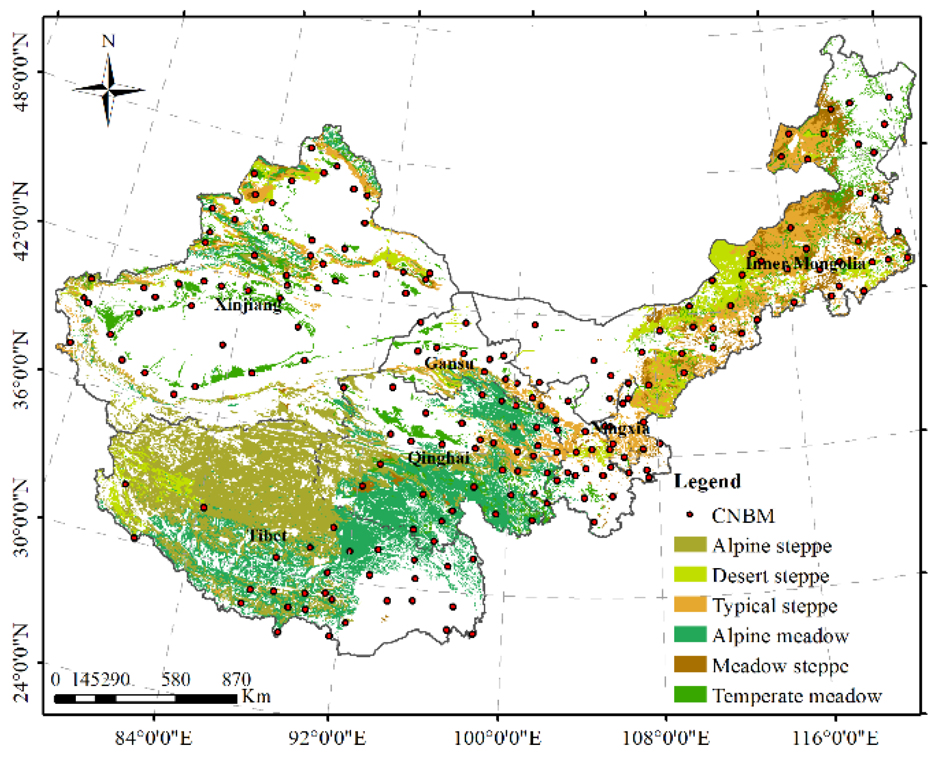
The study area (74.93–120.06° E, 29.25–49.51° N) is primarily located in the northwestern part of China and covers approximately 3.10 × 10⁶ m2 (Figure 1), which accounts for 79.7% of the grasslands in China. The area covers the regions of Inner Mongolia, Gansu, Ningxia, Xinjiang, Qinghai, and Tibet. The primary grassland types in the study area are alpine, temperate, and mountain grasslands. In detail, the alpine steppes and alpine meadows are on the Tibetan Plateau (TP); desert, typical, and meadow steppes are on the Inner Mongolian Plateau; and the mountain meadows are in the Xinjiang area [45]. The climate is arid and semiarid with an annual mean temperature (AMT) and annual mean precipitation (AMP), which range from −6.2 to 8.8 °C and from 92.3 to 694.0 mm, respectively, in the study area [45].
2.2. NDVI Database
We analyzed the plant phenology trends on the Tibetan Plateau from 1985 to 2010 using GIMMS3g NDVI remote sensing data sets with a spatial resolution of 0.083°, which were compiled by merging segments (data strips) during a half-month period, using the maximum value composites (MVC) method [46]. These data were corrected for calibration, view geometry, and volcanic aerosols, and have been verified using a stable desert control point.
2.3. Climate Database
Climatic data were collected from the Meteorology Information Center of the Chinese National Bureau of Meteorology (CNBM) (http://data.cma.cn/). Figure 1 shows the locations of the national standards of meteorology (Figure 1). The primary climatic factors (AMT and AMP) of the National Standard of Meteorology Observatories (1985–2010) were included in the document. Moreover, the spatial interpolation of AMT and AMP was generated in ArcGIS 10.2 (ESRI, Inc., Redlands, CA, USA) with the kriging interpolation method, in order to create 0.05° resolution climatic factors.
2.4. SOS, EOS, POS, and LOS Were Obtained with the Retrieval Method
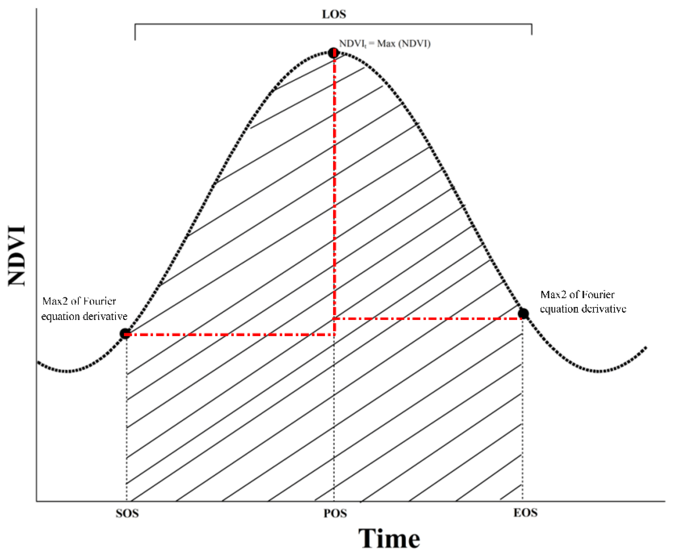
Four indicators, that is, the start of the growing season (SOS), peak of the growing season (POS), end of the growing season (EOS), and length of the growing season (LOS), were employed in describing the phenology (Figure 2). We derived the phenology indicators using the GIMMS 3g NDVI data set covering the period 1985–2010, because the plants in China’s grassland ecosystems only have one growing season in a year. To smooth the NDVI data set, the Fourier Series Model was applied as Equation (1).
In Equation (1), y indicates the fitted, smoothed NDVI value; a0 models a constant (intercept) term in the data; w is the fundamental frequency of the data series; and n is the number of terms in the series. For forest, shrub, and steppe, acceptable model results are obtained when n is equal to 1. Then, the SOS, POS, and EOS were determined using the derivatives of the fitted Fourier equation. As illustrated in Figure 2, SOS was defined as the Julian day when the derivative reached the highest value; POS was the Julian day when the maximum NDVI estimated by the fitted Fourier function appeared; EOS was the corresponding Julian day when the derivative of the fitted Fourier function obtained its minimum value; and LOS equaled the difference between EOS and SOS.
2.5. Data Analyses
To analyze the temporal and spatial dynamics of the phenology, and to reveal the relationships between the phenology and climatic factors, the least squares method was employed in this analysis. The change tendency of phenology and the spatial correlation relationships between phenology and climatic factors were analyzed by the least square method.
A redundancy analysis (RDA) in the software of R (R Core Development Team, R Foundation for Statistical Computing, Vienna, Austria) was used to determine the climatic factors for the variation of the phenology indicators, with the determinants (p < 0.05). RDA is a linear canonical ordination method and is widely used to identify the patterns of the dynamics in the response variables [47]. RDA is an effective way to evaluate the relationships among multiple interacting variables, which are also closely associated with the potential explanatory variables [48,49]. Finally, linear regression analysis was applied to develop the correlations between the phenology indicators and climatic factors in the software SigmaPlot 10.0 (Systat Software, Inc., Chicago, IL, USA).
3. Results
3.1. Dynamics and Relationships of Plant Phenology, AMT, and AMP across China’s Grasslands
3.1.1. Spatial Distribution of Plant Phenology, AMT, and AMP in China’s Grasslands
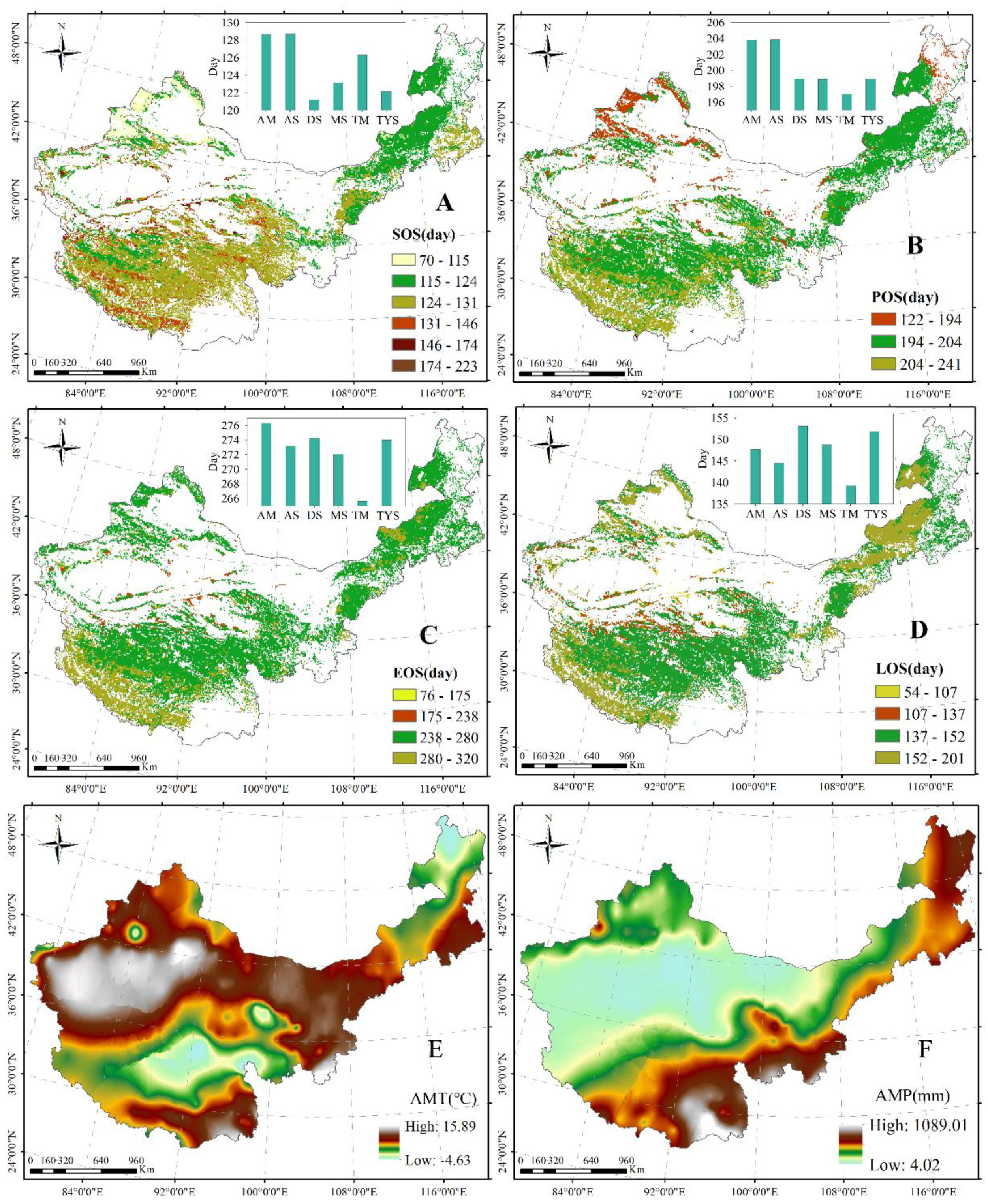
The spatial distribution patterns and plant phenology in different grasslands are shown in Figure 3. From northeast to southwest, the SOS and EOS were gradually delayed. Moreover, from northwest to southeast, the POS was gradually delayed. From the margin to the center of the study area, the LOS gradually shortened. The SOS was primarily observed from the 115th to 130th day from 1 January, which was distributed in Inner Mongolia and the TP, with the lowest (121) and highest (129) values in the desert steppe and alpine steppe, respectively (Figure 3A). The POS primarily occurred between days 190 and 210 from 1 January, and was also mostly distributed along Inner Mongolia to the TP, with the lowest (197) and highest (204) values from 1 January occurring in the temperate meadow and alpine steppe, respectively (Figure 3B). The EOS was primarily found between days 240 and 290 from January 1, and was presented in most regions in the study area and the lowest (265) and highest (273) values of EOS from 1 January were found in temperate meadow and alpine meadow, respectively (Figure 3C). The longer LOS was centrally distributed on the edge of the study area, with values between days 152 and 201, and the values from days 137 to 152 were primarily observed in the center of the TP and the east and the southwest of Inner Mongolia (Figure 3D). Additionally, the highest (153) and lowest (139) LOS values were found in desert steppe and temperate meadow, respectively.
Furthermore, the results indicated that the value of the AMT (1985–2010) ranged from −4.63 to 15.89 °C. A relatively low AMT was observed in the center of the TP and north of Inner Mongolia, and a relatively high AMT was found in the corridor of Hexi–Xinjiang and south of the TP (Figure 3E). Additionally, the AMP decreased toward the south–north on the TP, toward the north–south in Xinjiang, and toward the east–west in the study area, with the AMP ranging from 4.02 to 1089.01 mm (Figure 3F).
3.1.2. Dynamics of Plant Phenology, AMT, and AMP in China’s Grasslands
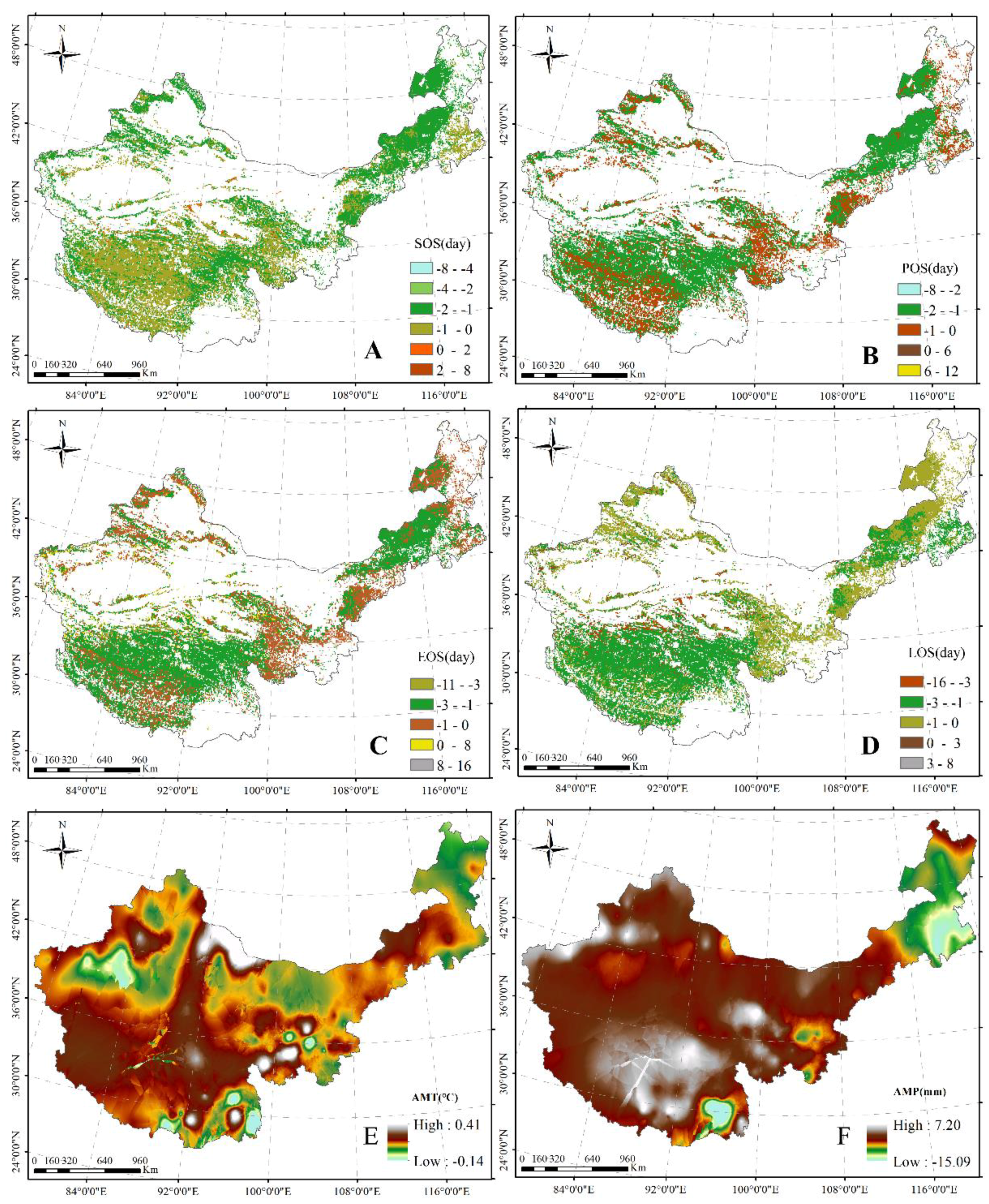
The SOS showed an advanced trend in most regions across China’s grasslands, with primarily advanced values of 0–2 days (Figure 4A). Similarly, the POS and EOS showed an advanced tendency across China’s grasslands; advanced values of 1–2 days were primarily found in the center of the TP and Inner Mongolia, and those of 0–1 day were primarily observed in the east and south of Inner Mongolia, in the east and south of the TP, and in the north of Xinjiang (Figure 4B,C). Additionally, the LOS presented a shortened trend over China’s grasslands; advanced values of 1–3 days were centrally distributed in the TP and mid Inner Mongolia, and those of 0–1 day were primarily found in the north and south of Inner Mongolia, in the east of the TP, and in most regions in Xinjiang (Figure 4D). In general, the SOS, POS, and EOS came early, with the variation amplitude of 0.54 days/year, 0.64 days/year, and 0.65 days/year, respectively. The LOS shortened at a rate of 0.62 days/year.
Moreover, the changed values of AMT showed variation from −0.14 to 0.41 °C, and the AMT presented a tendency of increase across China’s grasslands, except for the regions in the north of Inner Mongolia, the south of the TP, and the center of Xinjiang (Figure 4E). The dynamics of AMP were observed between −15.09 and 7.20 mm during the study period, and the decreases in AMP were primarily distributed in the northeast of Inner Mongolia and the south of the TP (Figure 4F). Simultaneously, the increases in AMP were primarily in the center of the TP and the north of Xinjiang (Figure 4F).
3.1.3. Responses of Plant Phenology to AMT and AMP across China’s Grasslands
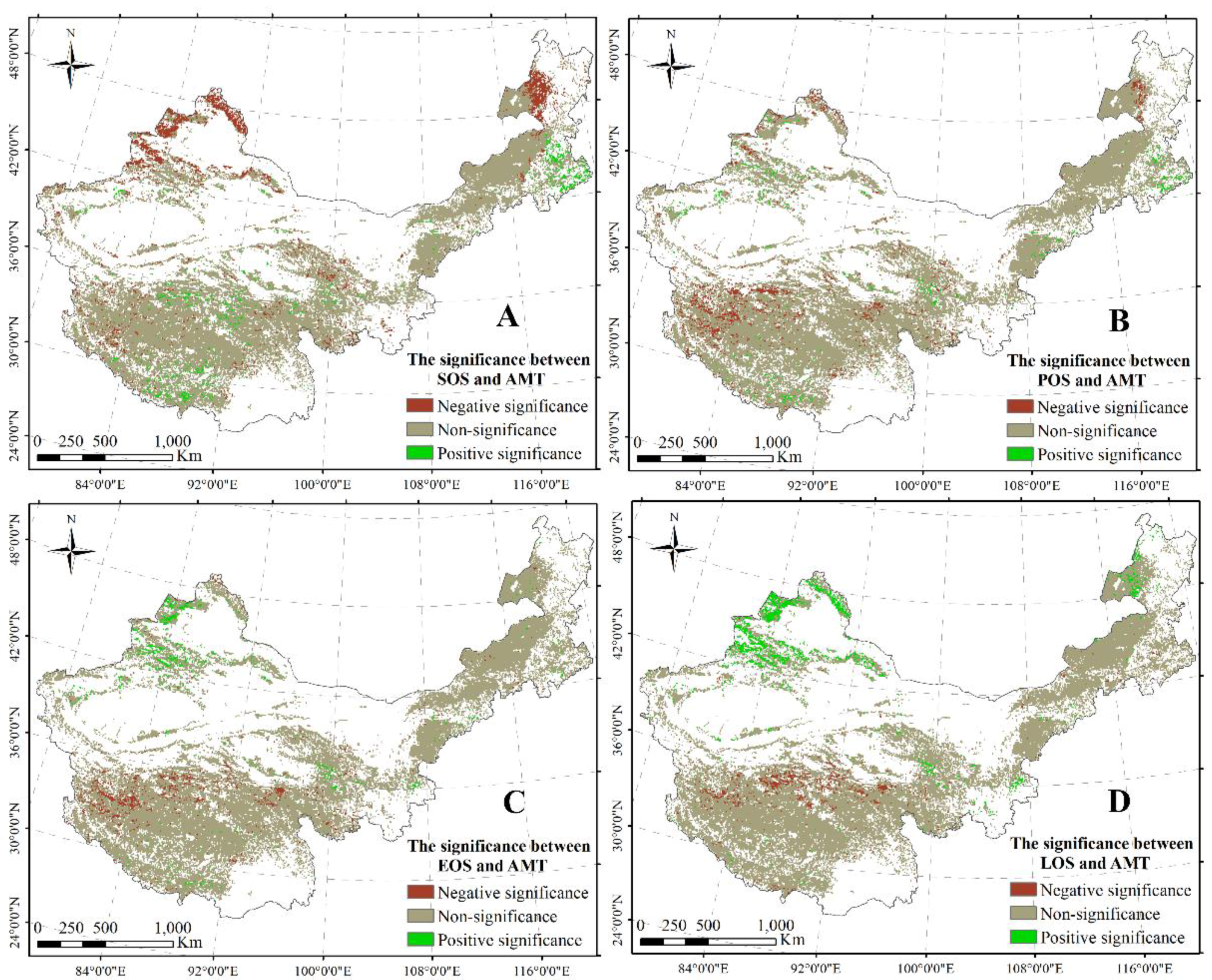
A significant negative correlation between the SOS and AMT was found in the east–north of Inner Mongolia, the north of Xinjiang, and a part of the area in the TP (Figure 5A). Moreover, a significant positive relationship between the SOS and AMT was revealed in the east–center of Inner Mongolia and the south and center of the TP (Figure 5A). Additionally, a significant negative correlation between the POS and AMT was found in the north of Xinjiang, the east–north of Inner Mongolia, and the center–west of the TP (Figure 5B). Similarly, between EOS/LOS and AMT, significant positive and negative relationships were revealed in the north of Xinjiang and the north of the TP (Figure 5C,D), respectively.
An obvious significant correlation between SOS and AMP was observed in most regions including the west–center of Inner Mongolia, the north of Xinjiang, and part of the regions on the TP (Figure 6A). Furthermore, a significant relationship between POS and AMP was primarily distributed in the center of Inner Mongolia, the north and east of the TP, and the north of Xinjiang (Figure 6B). A significant negative correlation between POS/EOS and AMP was found in the center of the TP and the east–north of Inner Mongolia (Figure 6B,C), with a significant relationship between EOS and AMP distributed in the center of the TP and the east–north of Inner Mongolia (Figure 6C). A significant negative correlation between LOS and AMP was primarily found in the center of the TP and the north of Inner Mongolia (Figure 6D). Simultaneously, a significant relationship between LOS and AMP was revealed in the east of the TP and part of the region in Inner Mongolia (Figure 6D).
3.2. Dynamics and Relationships in Plant Phenology, AMT, and AMP in Different Grassland Types
3.2.1. Dynamics of Plant Phenology in Different Grassland Types
To further reveal the dynamics of plant phenology, we analyzed the change rate of the phenology indicators in different grasslands across northern China. As shown in Table 1, the SOS in the meadow steppe (R2 = 0.26, p = 0.007) and typical steppe (R2 = 0.28, p = 0.005); the EOS in alpine steppe (R2 = 0.16, p < 0.05); and the LOS in alpine (R2 = 0.20, p < 0.05), meadow (R2 = 0.18, p < 0.05), and typical (R2 = 0.18, p < 0.05) steppes changed significantly.
3.2.2. Dynamics of AMT and AMP in Different Grassland Types
Based on the results in Table 1, we further revealed the dynamics of the climatic factors (Table 2) in grasslands with significantly changed phenology. The results indicated that the AMT in the alpine, meadow, and typical steppes showed a trend of increase, in which the average change rates of AMT were 0.05 °C/year, 0.06 °C/year, and 0.06 °C/year (Table 2), respectively. Conversely, a trend of decrease in AMP was observed in the grasslands of alpine, meadow, and typical steppes, with the average decrease in values of AMP of 1.75 mm/year, 0.60 mm/year, and 0.72 mm/year, respectively (Table 2).
3.2.3. Responses of Plant Phenology to AMT and AMP in Different Grassland Types
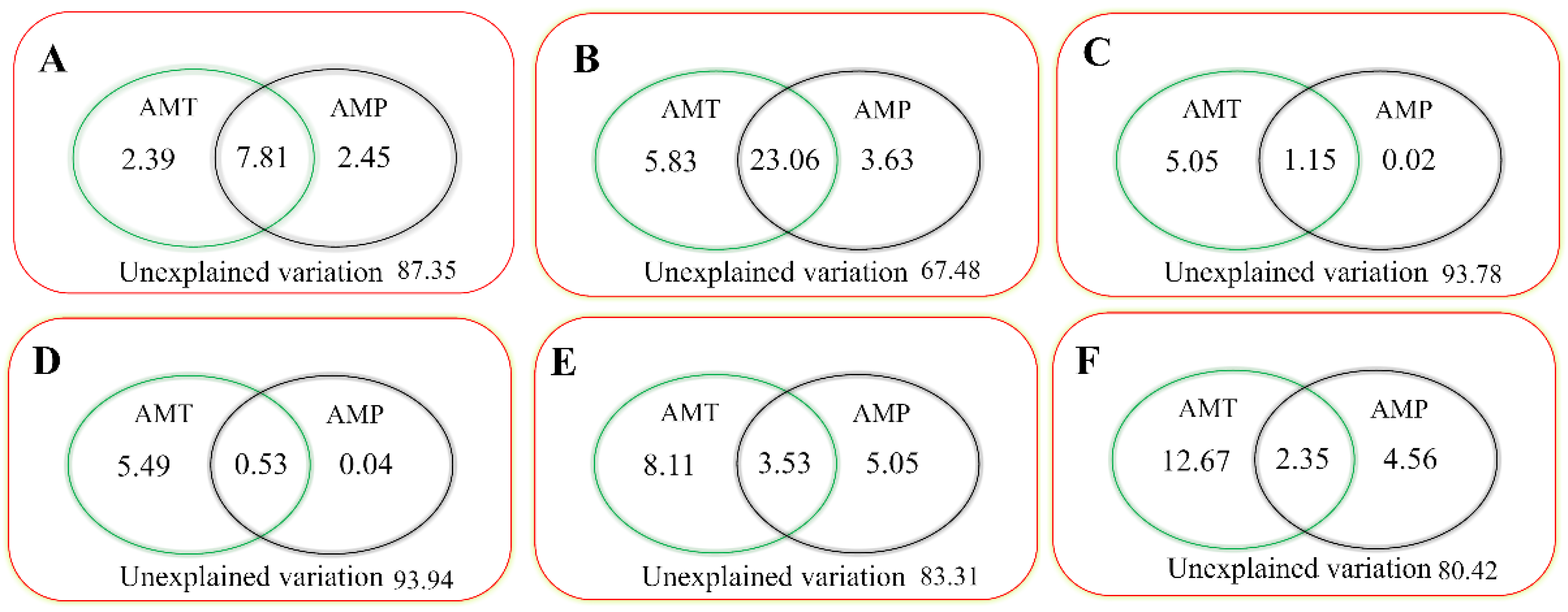
We further explored the response mechanisms between the phenology (significantly changed phenology in Table 1) and climatic factors by RDA. The results from the RDA showed that AMT and AMP together explained 12.65% (Figure 7A) and 32.52% (Figure 7B) of the variation of the SOS in the meadow steppe and typical steppe, respectively. Moreover, AMT and AMP together explained 6.22% of the dynamic of the EOS in the alpine steppe (Figure 7C). Additionally, AMT and AMP together explained 6.06% (Figure 7D), 16.69% (Figure 7E), and 19.58% (Figure 7F) of the variation of the LOS in the alpine, meadow, and typical steppes, respectively. Notably, AMP had a relatively larger influence on the variation of the SOS in the meadow steppe and typical steppe than that of AMT, whereas by contrast, AMT had a greater influence on the dynamics of the EOS in the alpine steppe. Similarly, AMT also had a relatively larger influence than that of AMP on the variation of the LOS in the alpine, meadow, and typical steppes.
4. Discussion
4.1. Spatial Distribution and Changes in Plant Phenology across China’s Grasslands
Our results indicated that the SOS, POS, and EOS advanced at the rates of 0.54 days/year, 0.64 days/year, and 0.65 days/year over China’s grasslands, respectively (Figure 4A–C). Moreover, the LOS shortened with the value of 0.62 days/year (Figure 4D). Consistent with our results, the observed data and remote sensing data demonstrate that plant phenology advanced in the past decades [50,51,52,53]. Specifically, the advanced SOS values for China (1982–1999) [54], the Eurasian continent (1981–1999) [55], the Northern Hemisphere (1982–2008) [56], and the world (1981–2003) [57] are 0.79 days/year, 0.33 days/year, 0.31 days/year, and 0.30 days/year, respectively.
Similarly, advanced EOS results are also found in many studies, in which the advanced rates of EOS are 0.37 days/year, 0.61 days/year, 0.23 days/year, and 0.50 days/year for China [58], the Eurasian continent [55], the Northern Hemisphere [56], and the world [57], respectively. Additionally, the inter-annual LOS presented a shortened trend in our results. Consistent with our results, the LOS shortened with the values of 1.16 days/year, 1.33 days/year, 0.56 days/year, and 0.38 days/year for China [54], the Eurasian continent [55], the Northern Hemisphere [27], and the world [55], respectively. In several studies, both observational and experimental, the POS shows an advanced trend in other regions [50,51,52,53,59,60].
In general, plant phenology showed significant changes in alpine, meadow, and typical steppes, which were primarily distributed in the center of the TP and Inner Mongolian Plateau. The maximum increased rates of AMT and AMP in the center of the TP (Figure 4E) and the maximum decrease in the AMP in the center of the Inner Mongolian Plateau (Figure 4F) might explain the corresponding significant changes in the phenology indicators (Table 1). Additionally, the alpine steppe in the north of the TP with a relatively low AMT and AMP was more sensitive to the dynamics of climatic factors than the alpine meadow in the southeast of the TP with a relatively high AMT and AMP, which might be another reason [35,36,46]. The non-significant changes to the phenology indicators in temperate meadows were primarily found in the north of Xinjiang Province, which might be explained because plant phenology at high altitudes is more sensitive and complicated than that at low altitude [31].
4.2. Control Mechanisms of Plant Phenology and Climate in Different Grasslands
Our results demonstrated that significant changes in plant phenology were revealed in the meadow steppe (R2 = 0.26, p = 0.007) and typical steppe (R2 = 0.28, p = 0.005) for the SOS, primarily distributed in Inner Mongolia (Table 1). Accompanying the differences in temperature and precipitation conditions, the SOS in the meadow steppe and typical steppe advanced gradually (Table 1). For the significantly changed SOS, an increased temperature in the meadow steppe (0.06 °C/year, Table 2) and typical steppe (0.06 °C/year, Table 2), which was primarily found in the center of the Inner Mongolian Plateau, accelerated the accumulation of heat and advanced the resumption of growth activity of plants, which affected the timing of the phenological phases [31]. Green-up onset tended to be advanced by the increasing temperature, and precipitation also exerted a stronger effect (Figure 7) on the SOS in the drier regions than that in others [32]. Thus, the SOS in the north of Xinjiang Province was significantly correlated with AMT and AMP (Figure 5A and Figure 6A). Similarly, advances in spring phenology are also reported in other studies [50,60,61,62]. Moreover, warming in springs and winters on the TP also continuously advanced the SOS at a rate of 1.04 days/year (1982–2011) [33], and an obvious positive correlation between the SOS and spring temperature was revealed in North America [63]. In summary, the starting growth of plant phenology was particularly sensitive to the change of temperature and precipitation [39,40,41,42,43,44].
Significantly advanced EOS was observed in the alpine steppe in the center of the TP (R2 = 0.16, p < 0.05; Table 1), and the AMT relatively explained most of the variation of the EOS (Figure 7). The warming temperature in the alpine steppe (0.05 °C/year, Table 2) therefore rapidly accelerated plant growth, resulting in an earlier completion of the growth in the steppe species [31]. Similarly, most regions in the center of the TP present a significant increase in temperature and a clear advance in the EOS by several weeks [64]. Thus, warming tended to be advanced for the EOS on the TP [64]. Because the growth of the alpine steppe on the TP is the most temperature-limited [65], plant growth is primarily sensitive to the dynamics in temperature [66,67,68,69]. Additionally, the dynamics of AMP in the alpine steppe might lead to the termination of plant growth to some extent, because water is the most important factor that affects plant growth [70,71,72].
The significantly advanced SOS in the meadow steppe and typical steppe, together with no significant change in the EOS, led to the gradual extension of the LOS in the meadow steppe (R2 = 0.18, p < 0.05) and typical steppe (R2 = 0.18, p < 0.05; Table 1). By contrast, the significantly advanced EOS, together with no significant change in the alpine steppe, accounted for the shortening of the LOS in the alpine steppe (R2 = 0.20, p < 0.05; Table 1). The variation of the LOS in the north of Xinjiang Province was positively correlated with AMT (Figure 5A), because of the significant relationship between AMT and SOS (Figure 5D), and warming temperature is beneficial to the extension of plant growth [34,54,61,64]. For example, an increase in AMT by 1 °C resulted in an extension of five days in Europe [61]; and across north China, a warming during March to early May by 1 °C led to an extension of the SOS by 7.5 days [54], whereas an increase of AMT by 1 °C from mid-August to early October generated a delay of 3.8 days in the EOS [54].
4.3. Limitations of the Current Study
Although a part of the variation in the phenology indicators was explained by climatic factors, in our study, other determinant factors might have had an effect on the dynamics of plant phenology, such as evapotranspiration, solar radiation, and soil properties (soil water content, soil total carbon, soil total nitrogen, soil total phosphorus, soil available nitrogen, soil available phosphorus, and soil microorganisms, among others). Because the effects of climatic factors on soil nutrients and the activity of soil microbes are closely related to the growth of plants, future research should devote more attention to the linkages between plant phenology and soil factors. For example, experiments on warming and simulating extreme rainfall are important to reveal how the phenology indicators (SOS, POS, EOS, and LOS) respond to changes in global climate and soil properties.
5. Conclusions
This study systematically revealed the spatiotemporal variation of plant phenology indicators (SOS, POS, EOS, and LOS) across China’s grasslands during 1985 to 2010. For the average phenology indicators over northern China, from the northeast to southwest, the SOS and EOS were gradually delayed. From the northwest to southeast, the POS was gradually delayed. From the margin to the center of the study area, the LOS gradually shortened. For the dynamics of the phenology indicators, the SOS, POS, and EOS presented an advanced tendency across China’s grasslands. Additionally, a shortening trend of the LOS over China’s grasslands was observed.
The SOS in the meadow steppe and typical steppe, and the EOS in the alpine steppe exhibited significantly advanced trends from 1985 to 2010. Moreover, the LOS showed significantly shortened trends in the meadow steppe and typical steppe, primarily distributed in Inner Mongolia, and the LOS underwent a lengthening trend in the alpine steppe as primarily revealed on the TP. The inter-annual climate changes of AMT and AMP in China’s grasslands accounted for the significantly dynamic SOS in the meadow steppe (12.65%) and typical steppe (32.52%); the EOS in the alpine steppe (6.22%); and the LOS in the alpine (6.06%), meadow (16.69%), and typical (19.58%) steppes. Thus, the changes in the plant phenology under climate change are critical requirements for the carbon cycle dynamics in these grassland ecosystems.
Author Contributions
T.Z. contributed to the study design; and J.W. and P.P. were involved in drafting the manuscript, approving the final draft, and agree to be accountable for the work. All of the authors read and approved the final manuscript.
Funding
This research was funded by the West Light Foundation of The Chinese Academy of Sciences.
Acknowledgments
We would like to thank Huan Zhao for research assistance.
Conflicts of Interest
The authors declare no conflict of interest.
References
- You, X.Z.; Meng, J.H.; Zhang, M.; Dong, T.F. Remote Sensing Based Detection of Crop Phenology for Agricultural Zones in China Using a New Threshold Method. Remote Sens. 2013, 5, 3190–3211. [Google Scholar] [CrossRef] [Green Version]
- Root, T.L.; Price, J.T.; Hall, K.R.; Schneider, S.H.; Rosenzweig, C.; Pounds, J.A. Fingerprints of global warming on wild animals and plants. Nature 2003, 421, 57–60. [Google Scholar] [CrossRef] [PubMed]
- Piao, S.L.; Cui, M.D.; Chen, A.P.; Wang, X.H.; Ciais, P.; Liu, J.; Tang, Y. Altitude and temperature dependence of change in the spring vegetation green-up date from 1982 to 2006 in the Qinghai-Xizang Plateau. Agric. For. Meteorol. 2011, 151, 1599–1608. [Google Scholar] [CrossRef]
- Ding, M.J.; Li, L.H.; Zhang, Y.L.; Sun, X.M.; Liu, L.S.; Gao, J.G.; Wang, Z.; Li, Y. Start of vegetation growing season on the Tibetan Plateau inferred from multiple methods based on GIMMS and SPOT NDVI data. J. Geogr. Sci. 2015, 25, 131–148. [Google Scholar] [CrossRef] [Green Version]
- Prevey, J.S.; Seastedt, T.R. Seasonality of precipitation interacts with exotic species to alter composition and phenology of a semi-arid grassland. J. Ecol. 2014, 102, 1549–1561. [Google Scholar] [CrossRef] [Green Version]
- Lesica, P.; Kittelson, P.M. Precipitation and temperature are associated with advanced flowering phenology in a semi-arid grassland. J. Arid Environ. 2010, 74, 1013–1017. [Google Scholar] [CrossRef]
- Bradley, A.V.; Gerard, F.F.; Barbier, N.; Weedon, G.P.; Anderson, L.O.; Huntingford, C.; Aragão, L.E.; Zelazowski, P.; Arai, E. Relationships between phenology, radiation and precipitation in the Amazon region. Glob. Change Biol. 2011, 17, 2245–2260. [Google Scholar] [CrossRef]
- Hmimina, G.; Dufrene, E.; Pontailler, J.Y.; Delpierre, N.; Aubinet, M.; Caquet, B.; De Grandcourt, A.; Burban, B.; Flechard, C.; Granier, A.; et al. Evaluation of the potential of MODIS satellite data to predict vegetation phenology in different biomes: An investigation using ground-based NDVI measurements. Remote Sens. Environ. 2013, 132, 145–158. [Google Scholar] [CrossRef]
- Leeuwen, W.J.D.V.; Davison, J.E.; Casady, G.M.; Marsh, S.E. Phenological Characterization of Desert Sky Island Vegetation Communities with Remotely Sensed and Climate Time Series Data. Remote Sens. 2010, 2, 388–415. [Google Scholar] [CrossRef] [Green Version]
- Shen, M.G.; Piao, S.L.; Cong, N.; Zhang, G.X.; Janssens, I.A. Precipitation impacts on vegetation spring phenology on the Tibetan Plateau. Glob. Change Biol. 2015, 21, 3647–3656. [Google Scholar] [CrossRef] [PubMed] [Green Version]
- Han, G.F.; Xu, J.H. Land Surface Phenology and Land Surface Temperature Changes Along an Urban-Rural Gradient in Yangtze River Delta, China. Environ. Manag. 2013, 52, 234–249. [Google Scholar] [CrossRef] [PubMed]
- Wang, C.; Cao, R.Y.; Chen, J.; Rao, Y.H.; Tang, Y.H. Temperature sensitivity of spring vegetation phenology correlates to within-spring warming speed over the Northern Hemisphere. Ecol. Indic. 2015, 50, 62–68. [Google Scholar] [CrossRef]
- He, Z.B.; Du, J.; Zhao, W.Z.; Yang, J.J.; Chen, L.F.; Zhu, X.; Chang, X.; Liu, H. Assessing temperature sensitivity of subalpine shrub phenology in semi-arid mountain regions of China. Agric. For. Meteorol. 2015, 213, 42–52. [Google Scholar] [CrossRef]
- Brown, M.E.; Beurs, K.M.D.; Marshall, M. Global phenological response to climate change in crop areas using satellite remote sensing of vegetation, humidity and temperature over 26 years. Remote Sens. Environ. 2012, 126, 174–183. [Google Scholar] [CrossRef]
- Shen, M.G.; Zhang, G.X.; Cong, N.; Wang, S.P.; Kong, W.D.; Piao, S.L. Increasing altitudinal gradient of spring vegetation phenology during the last decade on the Qinghai-Tibetan Plateau. Agric. For. Meteorol. 2014, 189, 71–80. [Google Scholar] [CrossRef]
- Qiu, B.W.; Zhong, M.; Zeng, C.Y.; Tang, Z.H.; Chen, C.C. Effect of topography and accessibility on vegetation dynamic pattern in Mountain-hill Region. J. Mt. Sci. 2012, 9, 879–890. [Google Scholar] [CrossRef]
- Hwang, T.; Song, C.H.; Vose, J.M.; Band, L.E. Topography-mediated controls on local vegetation phenology estimated from MODIS vegetation index. Landsc. Ecol. 2011, 26, 541–556. [Google Scholar] [CrossRef]
- Brown, L.A.; Dash, J.; Ogutu, B.O.; Richardson, A.D. On the relationship between continuous measures of canopy greenness derived using near-surface remote sensing and satellite-derived vegetation products. Agric. For. Meteorol. 2017, 247, 280–292. [Google Scholar] [CrossRef]
- Hufkens, K.; Friedl, M.; Sonnentag, O.; Braswell, B.H.; Milliman, T.; Richardson, A.D. Linking near-surface and satellite remote sensing measurements of deciduous broadleaf forest phenology. Remote Sens. Environ. 2012, 117, 307–321. [Google Scholar] [CrossRef]
- Klosterman, S.T.; Hufkens, K.; Gray, J.M.; Melaas, E.; Sonnentag, O.; Lavine, I.; Mitchell, L.; Norman, R.; Friedl, M.A.; Richardson, A.D. Evaluating remote sensing of deciduous forest phenology at multiple spatial scales using PhenoCam imagery. Biogeosciences 2014, 11, 4305–4320. [Google Scholar] [CrossRef] [Green Version]
- Liu, Y.; Hill, M.J.; Zhang, X.; Wang, Z.; Richardson, A.D.; Hufkens, K.; Filippa, G.; Baldocchi, D.D.; Ma, S.; Verfaillie, J. Using data from Landsat, MODIS, VIIRS and PhenoCams to monitor the phenology of California oak/grass savanna and open grassland across spatial scales. Agric. For. Meteorol. 2017, 237, 311–325. [Google Scholar] [CrossRef]
- Melaas, E.K.; Sulla-Menashe, D.; Gray, J.M.; Black, T.A.; Morin, T.H.; Richardson, A.D.; Friedl, M.A. Multisite analysis of land surface phenology in North American temperate and boreal deciduous forests from Landsat. Remote Sens. Environ. 2016, 186, 452–464. [Google Scholar] [CrossRef]
- Robinson, N.P.; Allred, B.W.; Jones, M.O.; Moreno, A.; Kimball, J.S.; Naugle, D.E.; Erickson, T.A.; Richardson, A.D.; Thenkabail, P. A Dynamic Landsat Derived Normalized Difference Vegetation Index (NDVI) Product for the Conterminous United States. Remote Sens. 2017, 9, 863. [Google Scholar] [CrossRef]
- Benhadj, I.; Duchemin, B.; Maisongrande, P.; Simonneaux, V.; Khabba, S.; Chehbouni, A. Automatic unmixing of MODIS multi-temporal data for inter-annual monitoring of land use at a regional scale (Tensift, Morocco). Int. J. Remote Sens. 2012, 33, 1325–1348. [Google Scholar] [CrossRef]
- Cook, B.I.; Smith, T.M.; Mann, M.E. The North Atlantic Oscillation and regional phenology prediction over europe. Glob. Change Biol. 2005, 11, 919–926. [Google Scholar] [CrossRef]
- Arrogante-Funes, P.; Novillo, C.; Romero-Calcerrada, R.; Vázquez-Jiménez, R.; Ramos-Bernal, R. Relationship between MRPV Model Parameters from MISRL2 Land Surface Product and Land Covers: A Case Study within Mainland Spain. ISPRS Int. J. Geo-Inf. 2017, 6, 353. [Google Scholar] [CrossRef]
- Gressler, E.; Jochner, S.; Capdevielle-Vargas, R.M.; Morellato, L.P.C.; Menzel, A. Vertical variation in autumn leaf phenology of Fagus sylvatica L. in southern Germany. Agric. For. Meteorol. 2015, 201, 176–186. [Google Scholar] [CrossRef]
- Sharma, R.; Tateishi, R.; Hara, K. A Biophysical Image Compositing Technique for the Global-Scale Extraction and Mapping of Barren Lands. ISPRS Int. J. Geo-Inf. 2016, 5, 225. [Google Scholar] [CrossRef]
- Dahlke, C.; Loew, A.; Reick, C. Robust Identification of Global Greening Phase Patterns from Remote Sensing Vegetation Products. J. Clim. 2012, 25, 8289–8307. [Google Scholar] [CrossRef]
- Verhegghen, A.; Bontemps, S.; Defourny, P. A global NDVI and EVI reference data set for land-surface phenology using 13 years of daily SPOT-VEGETATION observations. Int. J. Remote Sens. 2014, 35, 2440–2471. [Google Scholar] [CrossRef]
- Ding, M.J.; Zhang, Y.L.; Sun, X.M.; Liu, L.S.; Wang, Z.F.; Bai, W.Q. Spatiotemporal variation in alpine grassland phenology in the Qinghai-Tibetan Plateau from 1999 to 2009. Chin. Sci. Bull. 2013, 58, 396–405. [Google Scholar] [CrossRef]
- Yu, H.Y.; Luedeling, E.; Xu, J.C. Winter and spring warming result in delayed spring phenology on the Tibetan Plateau. Proc. Natl. Acad. Sci. USA 2010, 107, 22151–22156. [Google Scholar] [CrossRef] [PubMed] [Green Version]
- Shen, M.; Tang, Y.; Chen, J.; Zhu, X.; Zheng, Y. Influences of temperature and precipitation before the growing season on spring phenology in grasslands of the central and eastern Qinghai-Tibetan Plateau. Agric. For. Meteorol. 2011, 151, 1711–1722. [Google Scholar] [CrossRef]
- Zhang, G.L; Zhang, Y.J; Dong, J.W; Xiao, X.M. Green-up dates in the Tibetan Plateau have continuously advanced from 1982 to 2011. Proc. Natl. Acad. Sci. USA 2013, 110, 4309–4314. [Google Scholar] [CrossRef] [PubMed] [Green Version]
- Sun, J.; Cheng, G.W.; Li, W.P. Meta-analysis of relationships between environmental factors and aboveground biomass in the alpine grassland on the Tibetan Plateau. Biogeosciences 2013, 10, 1707–1715. [Google Scholar] [CrossRef]
- Sun, J.; Wang, H.M. Soil nitrogen and carbon determine the trade-off of the above- and below-ground biomass across alpine grasslands, Tibetan Plateau. Ecol. Indic. 2016, 60, 1070–1076. [Google Scholar] [CrossRef]
- Wang, C.Z.; Guo, H.D.; Zhang, L.; Liu, S.Y.; Qiu, Y.B.; Sun, Z.C. Assessing phenological change and climatic control of alpine grasslands in the Tibetan Plateau with MODIS time series. Int. J. Biometeorol. 2015, 59, 11–23. [Google Scholar] [CrossRef] [PubMed]
- Lu, L.L.; Li, Q.T.; Wang, C.Z.; Guo, H.D.; Zhang, L. Spatiotemporal Variations of Satellite-Derived Phenology in the Tibetan Plateau. In Proceedings of the 2012 IEEE International Geoscience and Remote Sensing Symposium (Igarss), Munich, Germany, 22–27 July 2012; pp. 6451–6454. [Google Scholar]
- Yu, H.Y.; Xu, J.C.; Okuto, E.; Luedeling, E. Seasonal Response of Grasslands to Climate Change on the Tibetan Plateau. PLoS ONE 2012, 7, e49230. [Google Scholar] [CrossRef] [PubMed]
- Yi, S.H.; Zhou, Z.Y. Increasing contamination might have delayed spring phenology on the Tibetan Plateau. Proc. Natl. Acad. Sci. USA 2011, 108, E94. [Google Scholar] [CrossRef] [PubMed]
- Zhang, G.L.; Dong, J.W.; Zhang, Y.J.; Xiao, X.M. Reply to Shen et al.: No evidence to show nongrowing season NDVI affects spring phenology trend in the Tibetan Plateau over the last decade. Proc. Natl. Acad. Sci. USA 2013, 110, E2330–E2331. [Google Scholar] [CrossRef] [PubMed]
- Shen, M.G.; Sun, Z.Z.; Wang, S.P.; Zhang, G.X.; Kong, W.D.; Chen, A.P.; Piao, S. No evidence of continuously advanced green-up dates in the Tibetan Plateau over the last decade. Proc. Natl. Acad. Sci. USA 2013, 110, E2329. [Google Scholar] [CrossRef] [PubMed]
- Dong, J.W.; Zhang, G.L.; Zhang, Y.J.; Xiao, X.M. Reply to Wang et al.: Snow cover and air temperature affect the rate of changes in spring phenology in the Tibetan Plateau. Proc. Natl. Acad. Sci. USA 2013, 110, E2856–E2857. [Google Scholar] [CrossRef] [PubMed]
- Wang, T.; Peng, S.S.; Lin, X.; Chang, J.F. Declining snow cover may affect spring phenological trend on the Tibetan Plateau. Proc. Natl. Acad. Sci. USA 2013, 110, E2854–E2855. [Google Scholar] [CrossRef] [PubMed] [Green Version]
- Yang, Y.; Fang, J.; Ji, C.; Datta, A.; Li, P.; Ma, W.; Mohammat, A.; Shen, H.; Hu, H.; Knapp, B.O.; et al. Stoichiometric shifts in surface soils over broad geographical scales: Evidence from China’s grasslands. Glob. Ecol. Biogeogr. 2014, 23, 947–955. [Google Scholar] [CrossRef]
- Sun, J.; Cheng, G.W.; Li, W.P.; Sha, Y.K.; Yang, Y.C. On the Variation of NDVI with the Principal Climatic Elements in the Tibetan Plateau. Remote Sens. 2013, 5, 1894–1911. [Google Scholar] [CrossRef] [Green Version]
- Almadani, S.; Ibrahim, E.; Abdelrahman, K.; Al-Bassam, A.; Al-Shmrani, A. Magnetic and seismic refraction survey for site investigation of an urban expansion site in Abha District, Southwest Saudi Arabia. Arab. J. Geosci. 2015, 8, 2299–2312. [Google Scholar] [CrossRef]
- Chen, Y.L.; Ding, J.Z.; Peng, Y.F.; Li, F.; Yang, G.B.; Liu, L.; Qin, S.Q.; Fang, K.; Yang, Y.H. Patterns and drivers of soil microbial communities in Tibetan alpine and global terrestrial ecosystems. J. Biogeogr. 2016, 43, 2027–2039. [Google Scholar] [CrossRef]
- Tang, W.; Zhou, T.; Sun, J.; Li, Y.; Li, W. Accelerated Urban Expansion in Lhasa City and the Implications for Sustainable Development in a Plateau City. Sustainability 2017, 9, 1499. [Google Scholar] [CrossRef]
- Myneni, R.B.; Keeling, C.D.; Tucker, C.J.; Asrar, G.; Nemani, R.R. Increased plant growth in the northern high latitudes from 1981 to 1991. Nature 1997, 386, 698–702. [Google Scholar] [CrossRef]
- Parmesan, C.; Yohe, G. A globally coherent fingerprint of climate change impacts across natural systems. Nature 2003, 421, 37–42. [Google Scholar] [CrossRef] [PubMed]
- Sherry, R.A.; Zhou, X.; Gu, S.; Rd, A.J.; Schimel, D.S.; Verburg, P.S.; Wallace, L.L.; Luo, Y. Divergence of reproductive phenology under climate warming. Proc. Natl. Acad. Sci. USA 2007, 104, 198–202. [Google Scholar] [CrossRef] [PubMed]
- Slayback, D.A.; Pinzon, J.E.; Los, S.O.; Tucker, C.J. Northern hemisphere photosynthetic trends 1982–99. Glob. Change Biol. 2010, 9, 1–15. [Google Scholar] [CrossRef]
- Shilong, P.; Fang, J.; Zhou, L.; Philippe, C.; Zhu, B. Variations in satellite-derived phenology in China’s temperate vegetation. Glob. Change Biol. 2010, 12, 672–685. [Google Scholar]
- Zhou, L.; Tucker, C.J.; Kaufmann, R.K.; Slayback, D.; Shabanov, N.V.; Myneni, R.B. Variations in northern vegetation activity inferred from satellite data of vegetation index during 1981 to 1999. J. Geophys. Res. Atmos. 2001, 106, 20069–20083. [Google Scholar] [CrossRef] [Green Version]
- Jeong, S.J.; Chang-Hoi, H.O.; Gim, H.J.; Brown, M.E. Phenology shifts at start vs. end of growing season in temperate vegetation over the Northern Hemisphere for the period 1982–2008. Glob. Change Biol. 2011, 17, 2385–2399. [Google Scholar] [CrossRef]
- Julien, Y.; Sobrino, J.A. Global land surface phenology trends from GIMMS database. Int. J. Remote Sens. 2009, 30, 3495–3513. [Google Scholar] [CrossRef]
- Zhang, X.; Friedl, M.A.; Schaaf, C.B.; Strahler, A.H.; Hodges, J.C.F.; Gao, F.; Reed, B.C.; Huete, A. Monitoring vegetation phenology using MODIS. Remote Sens. Environ. 2003, 84, 471–475. [Google Scholar] [CrossRef]
- Dunne, J.A.; Harte, J.; Taylor, K.J. Subalpine meadow flowering phenology responses to climate change: integrating experimental and gradient methods. Ecol. Monogr. 2003, 73, 69–86. [Google Scholar] [CrossRef]
- Bradley, N.L.; Leopold, A.C.; Ross, J.; Huffaker, W. Phenological changes reflect climate change in Wisconsin. Proc. Natl. Acad. Sci. USA 1999, 96, 9701–9704. [Google Scholar] [CrossRef] [PubMed] [Green Version]
- Chmielewski, F.M.; Rötzer, T. Response of tree phenology to climate change across Europe. Agric. For. Meteorol. 2001, 108, 101–112. [Google Scholar] [CrossRef]
- CAMILLE. Influences of species, latitudes and methodologies on estimates of phenological response to global warming. Glob. Change Biol. 2007, 13, 1860–1872. [Google Scholar]
- Menzel, A.; Fabian, P. Growing season extended in Europe. Nature 1999, 397, 659. [Google Scholar] [CrossRef]
- Wang, X.; Piao, S.; Ciais, P.; Li, J.; Friedlingstein, P.; Koven, C.; Chen, A. Spring temperature change and its implication in the change of vegetation growth in North America from 1982 to 2006. Proc. Natl. Acad. Sci. USA 2011, 108, 1240–1245. [Google Scholar] [CrossRef] [PubMed] [Green Version]
- Qin, X.; Sun, J.; Wang, X. Plant coverage is more sensitive than species diversity in indicating the dynamics of the above-ground biomass along a precipitation gradient on the Tibetan Plateau. Ecol. Indic. 2018, 84, 507–514. [Google Scholar] [CrossRef]
- Nemani, R.R.; Keeling, C.D.; Hashimoto, H.; Jolly, W.M.; Piper, S.C.; Tucker, C.J.; Myneni, R.B.; Running, S.W. Climate-driven increases in global terrestrial net primary production from 1982 to 1999. Science 2003, 300, 1560–1563. [Google Scholar] [CrossRef] [PubMed]
- Lucht, W.; Prentice, I.C.; Myneni, R.B.; Sitch, S.; Friedlingstein, P.; Cramer, W.; Bousquet, P.; Buermann, W.; Smith, B. Climatic Control of the High-Latitude Vegetation Greening Trend and Pinatubo Effect. Science 2002, 296, 1687–1689. [Google Scholar] [CrossRef] [PubMed] [Green Version]
- Piao, S.; Friedlingstein, P.; Ciais, P.; Zhou, L.; Chen, A. Effect of climate and CO2 changes on the greening of the Northern Hemisphere over the past two decades. Geophys. Res. Lett. 2006, 33, 265–288. [Google Scholar] [CrossRef]
- Braswell, B.H.; Schimel, D.S.; Linder, E.; Moore, B. The Response of Global Terrestrial Ecosystems to Interannual Temperature Variability. Science 1997, 278, 870–872. [Google Scholar] [CrossRef]
- Austin, A.T.; Vitousek, P.M. Nutrient dynamics on a precipitation gradient in Hawai’i. Oecologia 1998, 113, 519–529. [Google Scholar] [CrossRef] [PubMed]
- Paruelo, J.M.; Lauenroth, W.K.; Burke, I.C.; Sala, O.E. Grassland Precipitation-Use Efficiency Varies Across a Resource Gradient. Ecosystems 1999, 2, 64–68. [Google Scholar] [CrossRef]
- Halse, S.A.; Scanlon, M.D.; Cocking, J.S.; Smith, M.J.; Kay, W.R. Factors affecting river health and its assessment over broad geographic ranges: The Western Australian experience. Environ. Monit. Assess. 2007, 134, 161–175. [Google Scholar] [CrossRef] [PubMed]
Figure 1.
The study area is primarily located in the northwestern part of China.

Figure 2.
Illustration of the normalized difference plant index (NDVI) ratio method used to model the growing season (SOS), peak of the growing season (POS), end of the growing season (EOS), and length of the growing season (LOS).
Figure 2.
Illustration of the normalized difference plant index (NDVI) ratio method used to model the growing season (SOS), peak of the growing season (POS), end of the growing season (EOS), and length of the growing season (LOS).

Figure 3.
Average spatial distribution of the grassland SOS (A); POS (B); EOS (C); LOS (D); annual mean temperature (AMT) (E); and annual mean precipitation (AMP) (F) between 1985 and 2010 in northern China. AM, AS, DS, MS, TM, and TYS represent the alpine meadow, alpine steppe, desert steppe, meadow steppe, temperate meadow, and typical steppe, respectively.

Figure 4.
Spatial distribution of inter-annual change trends of grassland SOS (A); POS (B); EOS (C); LOS (D); AMT (E); and AMP (F) from 1985 to 2010 in northern China.
Figure 4.
Spatial distribution of inter-annual change trends of grassland SOS (A); POS (B); EOS (C); LOS (D); AMT (E); and AMP (F) from 1985 to 2010 in northern China.

Figure 5.
Significant correlations between SOS and AMT (A); between POS and AMT (B); between EOS and AMT (C); and between LOS and AMT (D). The significance level is 0.05.
Figure 5.
Significant correlations between SOS and AMT (A); between POS and AMT (B); between EOS and AMT (C); and between LOS and AMT (D). The significance level is 0.05.

Figure 6.
Significant correlations between SOS and AMP (A); between POS and AMP (B); between EOS and AMP (C); and between LOS and AMP (D). The significance level is 0.05.
Figure 6.
Significant correlations between SOS and AMP (A); between POS and AMP (B); between EOS and AMP (C); and between LOS and AMP (D). The significance level is 0.05.
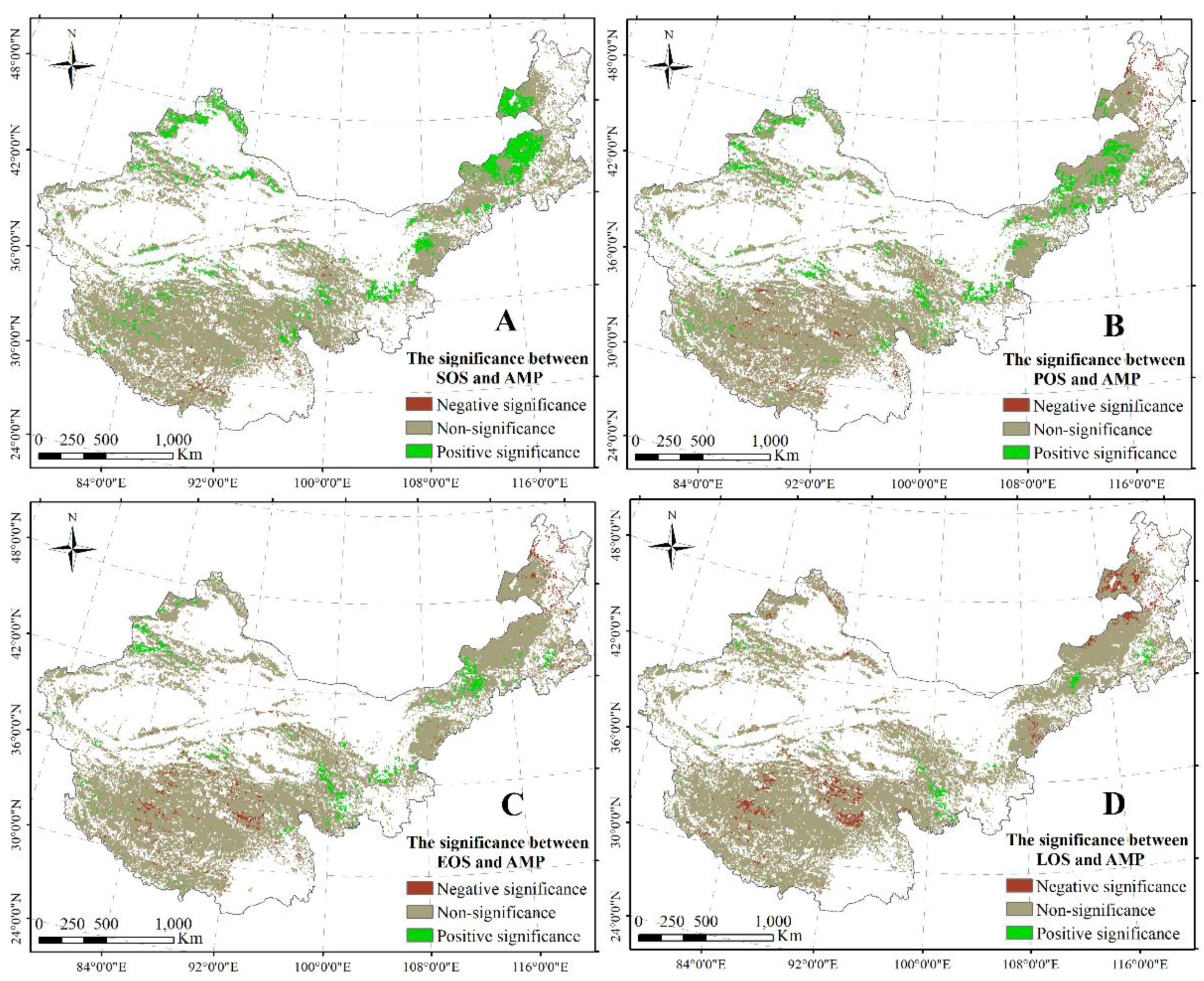
Figure 7.
Variance in phenology that might be explained (%) by climatic factors (AMT and AMP) using redundancy analysis. Graphs (A–F) refer to the SOS in the meadow and typical steppes; the EOS in the alpine steppe; and the LOS in the alpine, meadow, and typical steppes that might be explained by climatic factors, respectively.


Table 1.
The variation of vegetation phenology in different grasslands across northern China (1985–2010). y is the phenology indicator (start of the growing season [SOS], peak of the growing season [POS], end of the growing season [EOS], and length of the growing season [LOS]) ; x is the years 1985–2010; R2 is the fitting optimization index; p is the probability to reject the null hypothesis; y0 is the intercept; and a is the slope.
| Indicator | Grasslands | y = ax + y0 | R2 | p | Mean (day) |
|---|---|---|---|---|---|
| SOS (day) | Alpine meadow | y = 0.0066x + 115.5370 | 0.0009 | 0.8856 | 128.6547 |
| Alpine steppe | y = 0.0805x − 32.0302 | 0.0488 | 0.2784 | 128.7045 | |
| Desert steppe | y = −0.0453x + 211.6438 | 0.0145 | 0.5586 | 121.2055 | |
| Meadow steppe | y = −0.1264x + 375.7233 | 0.2648 | 0.0072 ** | 123.1431 | |
| Temperate meadow | y = −0.0061x + 138.4402 | 0.0006 | 0.9081 | 126.3115 | |
| Typical steppe | y = −0.1559x + 433.6264 | 0.281 | 0.0053 ** | 122.1544 | |
| POS (day) | Alpine meadow | y = −0.0353x + 274.3249 | 0.0125 | 0.5866 | 203.8044 |
| Alpine steppe | y = −0.1289x + 461.3085 | 0.0604 | 0.2263 | 203.8654 | |
| Desert steppe | y = −0.0910x + 380.6512 | 0.0606 | 0.2255 | 198.9293 | |
| Meadow steppe | y = −0.0520x + 302.7789 | 0.0561 | 0.2442 | 198.9030 | |
| Temperate meadow | y = −0.0029x + 202.8453 | 0.0002 | 0.9437 | 197.0213 | |
| Typical steppe | y = −0.0564x + 311.6396 | 0.0524 | 0.2605 | 198.9553 | |
| EOS (day) | Alpine meadow | y = −0.0981x + 472.2792 | 0.0411 | 0.3207 | 276.2977 |
| Alpine steppe | y = −0.3772x + 1026.7458 | 0.1614 | 0.0419 ** | 273.2050 | |
| Desert steppe | y = −0.0896x + 453.2871 | 0.0372 | 0.3450 | 274.3001 | |
| Meadow steppe | y = 0.0737x + 124.8830 | 0.043 | 0.3095 | 272.0691 | |
| Temperate meadow | y = 0.0490x + 167.7751 | 0.0216 | 0.4741 | 265.6026 | |
| Typical steppe | y = 0.0648x + 144.5951 | 0.029 | 0.4053 | 273.9888 | |
| LOS (day) | Alpine meadow | y = −0.1047x + 356.7421 | 0.0546 | 0.2505 | 147.6430 |
| Alpine steppe | y = −0.4577x + 1058.7759 | 0.202 | 0.0213 ** | 144.5005 | |
| Desert steppe | y = −0.0443x + 241.6433 | 0.0061 | 0.7051 | 153.0946 | |
| Meadow steppe | y = 0.1866x − 223.9604 | 0.1807 | 0.0304 ** | 148.7567 | |
| Temperate meadow | y = 0.0550x + 29.3350 | 0.0128 | 0.5816 | 139.2911 | |
| Typical steppe | y = 0.2207x − 289.0314 | 0.1761 | 0.0329 ** | 151.8344 |
** Represents significance at the level of 0.05.
Table 2.
The variation of climatic factors (annual mean temperature [AMT] and annual mean precipitation [AMP]) in three grasslands (1985–2010). The Mean, Min, Max. and Std are the average, minimum, maximum, and standard deviation values, respectively, of the AMT or AMP in corresponding grasslands from 1985 to 2010.
| Factor | Grasslands | Mean | Min | Max | Range | Std |
|---|---|---|---|---|---|---|
| AMT (°C/year) | Alpine steppe | 0.05 | 0.00 | 0.23 | 0.23 | 0.02 |
| Meadow steppe | 0.06 | −0.02 | 0.17 | 0.19 | 0.02 | |
| Typical steppe | 0.06 | −0.01 | 0.18 | 0.19 | 0.02 | |
| AMP (mm/year) | Alpine steppe | −1.75 | −7.76 | 4.29 | 12.05 | 2.39 |
| Meadow steppe | −0.60 | −7.93 | 3.98 | 11.91 | 1.83 | |
| Typical steppe | −0.72 | −7.50 | 3.98 | 11.48 | 2.53 |
© 2018 by the authors. Licensee MDPI, Basel, Switzerland. This article is an open access article distributed under the terms and conditions of the Creative Commons Attribution (CC BY) license (http://creativecommons.org/licenses/by/4.0/).
Share and Cite
MDPI and ACS Style
Wang, J.; Zhou, T.; Peng, P. Phenology Response to Climatic Dynamic across China’s Grasslands from 1985 to 2010. ISPRS Int. J. Geo-Inf. 2018, 7, 290. https://0-doi-org.brum.beds.ac.uk/10.3390/ijgi7080290
AMA Style
Wang J, Zhou T, Peng P. Phenology Response to Climatic Dynamic across China’s Grasslands from 1985 to 2010. ISPRS International Journal of Geo-Information. 2018; 7(8):290. https://0-doi-org.brum.beds.ac.uk/10.3390/ijgi7080290
Chicago/Turabian StyleWang, Jun, Tiancai Zhou, and Peihao Peng. 2018. "Phenology Response to Climatic Dynamic across China’s Grasslands from 1985 to 2010" ISPRS International Journal of Geo-Information 7, no. 8: 290. https://0-doi-org.brum.beds.ac.uk/10.3390/ijgi7080290
Note that from the first issue of 2016, this journal uses article numbers instead of page numbers. See further details here.