Article

Improving Tree Species Classification Using UAS Multispectral Images and Texture Measures

1
Department of Civil and Environmental Engineering, Politecnico di Milano, 20133 Milano, Italy
2
Department of Civil, Chemical and Environmental Engineering, Università degli Studi di Genova, 16145 Genova, Italy
*
Author to whom correspondence should be addressed.
ISPRS Int. J. Geo-Inf. 2018, 7(8), 315; https://0-doi-org.brum.beds.ac.uk/10.3390/ijgi7080315
Submission received: 14 June 2018 / Revised: 16 July 2018 / Accepted: 30 July 2018 / Published: 3 August 2018
(This article belongs to the Special Issue Applications and Potential of UAV Photogrammetric Survey)

Abstract

:
This paper focuses on the use of ultra-high resolution Unmanned Aircraft Systems (UAS) imagery to classify tree species. Multispectral surveys were performed on a plant nursery to produce Digital Surface Models and orthophotos with ground sample distance equal to 0.01 m. Different combinations of multispectral images, multi-temporal data, and texture measures were employed to improve classification. The Grey Level Co-occurrence Matrix was used to generate texture images with different window sizes and procedures for optimal texture features and window size selection were investigated. The study evaluates how methods used in Remote Sensing could be applied on ultra-high resolution UAS images. Combinations of original and derived bands were classified with the Maximum Likelihood algorithm, and Principal Component Analysis was conducted in order to understand the correlation between bands. The study proves that the use of texture features produces a significant increase of the Overall Accuracy, whose values change from 58% to 78% or 87%, depending on components reduction. The improvement given by the introduction of texture measures is highlighted even in terms of User’s and Producer’s Accuracy. For classification purposes, the inclusion of texture can compensate for difficulties of performing multi-temporal surveys.

1. Introduction

Unmanned Aircraft Systems (UAS) are rapidly evolving technologies that are nowadays used in a wide range of geospatial surveys and natural resources management applications. The UAS now available differ in dimension, shape, payload, flight height, and duration. The attention of the most of operators is mainly focused on mini and micro UAS, because of their easiness of use and versatility. Over the last few years, small fixed-wing, helicopters, and multi-rotor Unmanned Aerial Vehicles (UAV), equipped with Global Navigation Satellite System and Inertial Navigation System (GNSS/INS), with a total weight of 5 kg or less (Micro-UAV [1]) are increasingly being used for different scientific environmental surveys [2,3,4], including Photogrammetry and Remote Sensing (RS) purposes [1].
The low operational altitude of UAS surveys results in the generation of ultra-high resolution data [5], while their reduced physical size allows their rapid deployment, improving their capability to exploit limited windows of opportunity [6]. Furthermore, the low cost of platforms and navigation systems together with the variety of available sensors make the UAS suitable to be employed in many situations where a traditional vehicle (i.e., airplane) would be too expensive to justify its use.
UAS mounting multispectral digital cameras offer particular advantages over other remote sensing platforms. Their capability to generate ultra-high resolution imagery [7] at flexible temporal scales makes the UAS suitable to fill the gap between finer scale field samples and coarser scale aerial or satellite imagery. In particular, UAS have already given evidence of being an appropriate platform for mapping agricultural crops and forests. Configurations composed of UAV and consumer digital cameras were successfully applied to map Mediterranean forests [5], arid rangelands [8,9], Antarctic moss beds [10,11] and aquatic weeds [12]. UAS have the potential for mapping and monitoring endangered ecosystems and invasive or dominant tree species [13,14,15].
Many tests have been made to extend the use of processing techniques commonly used in remote sensing, for instance color spaces transformations or use of band ratios, derived indices, and texture variables for image interpretation. In precision agriculture applications, Vegetation Indices (VI), and texture measures derived from multispectral UAS imagery are widely used for weed detection [16,17,18]; Liu et al. [19] developed a method for the estimation of rice lodging, by combining indices derived from visible, and thermal infrared UAS data.
Several studies proved that the addition of spatial variability information, with texture measures, can significantly improve the accuracy of classification [20]. While in satellite remote sensing texture features are mainly used in coarse land cover mapping [21], in ultra-high resolution UAS imagery, texture measures enable to differentiate surfaces at a finer level, increasing the number of distinguishable classes (e.g., different types of vegetation), enhancing class separatebility and classification accuracy. In particular, Laliberte and Rango [22] employed texture components derived from UAS imagery in an object-based image analysis; Kelcey and Lucieer [3] and Feng et al. [23] recently performed processing of UAS datasets incorporating texture features.
Following the aforementioned researches, this work develops a study case to assess the capabilities of UAS survey to discriminate tree species. As respect to previous works [14,24], which focus on the detection of specific invasive species, our intent was to evaluate strategies for mapping several tree species. To this purpose, a plant nursery was identified as a suitable study area: a great tree species variety was concentrated in a small area, and ground truth data were easily accessible. Some well-known and consolidate RS pixel-based procedures were exploited, such as Principal Component Analysis and Maximum Likelihood classifier, with the intent to evaluate RS routines applied on ultra-high resolution images. Aim of the work is to test processing methods to identify tree species using multispectral UAS imagery with pixel-based classification and to evaluate if the inclusion of derived band as well as texture features significantly improves classification accuracy.

2. Materials and Methods

The flowchart, describing the general processing steps discussed in the next sections, is proposed in Figure 1.

2.1. Study Site and Instruments

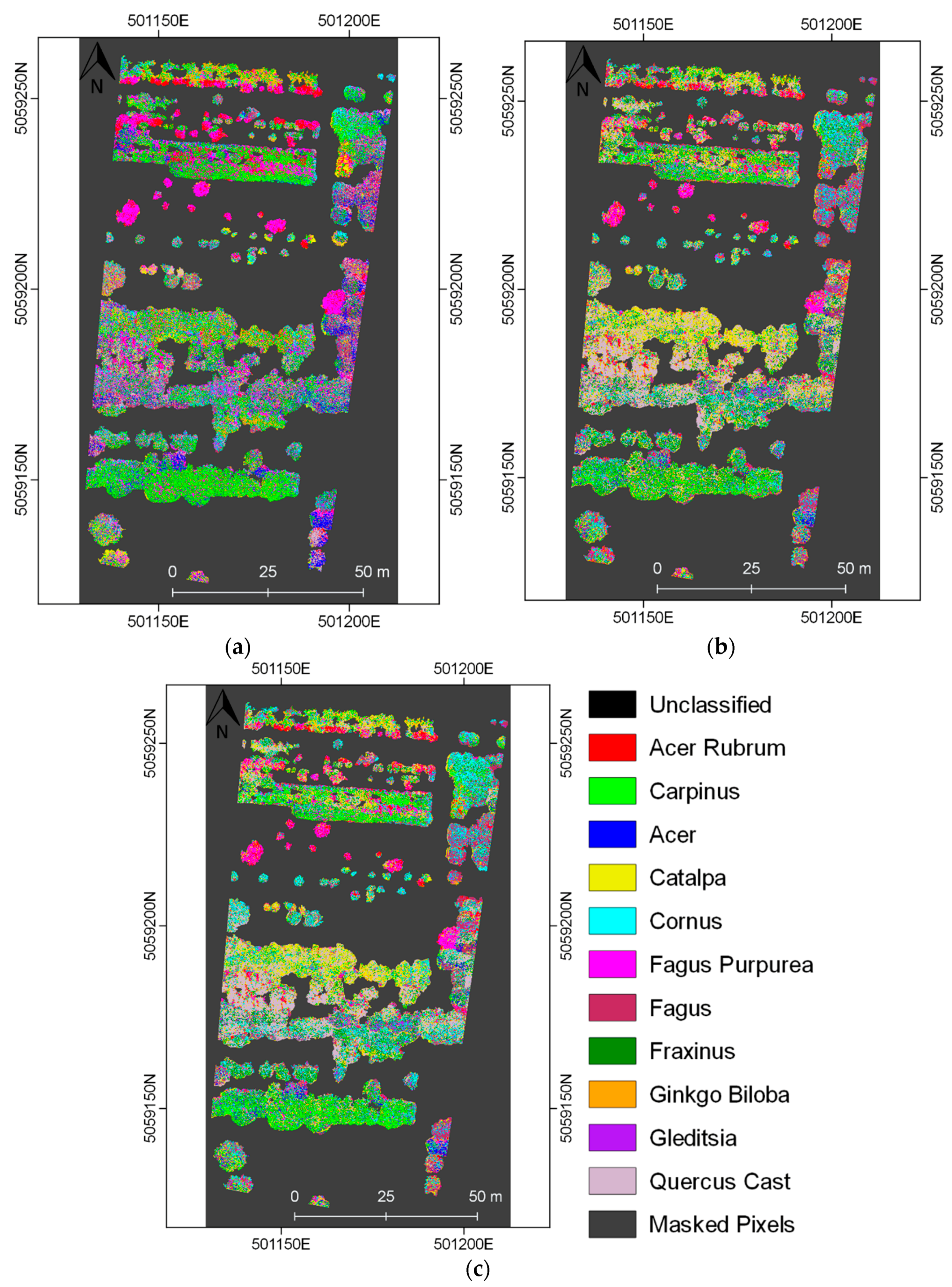
A small area of 215 × 115 m
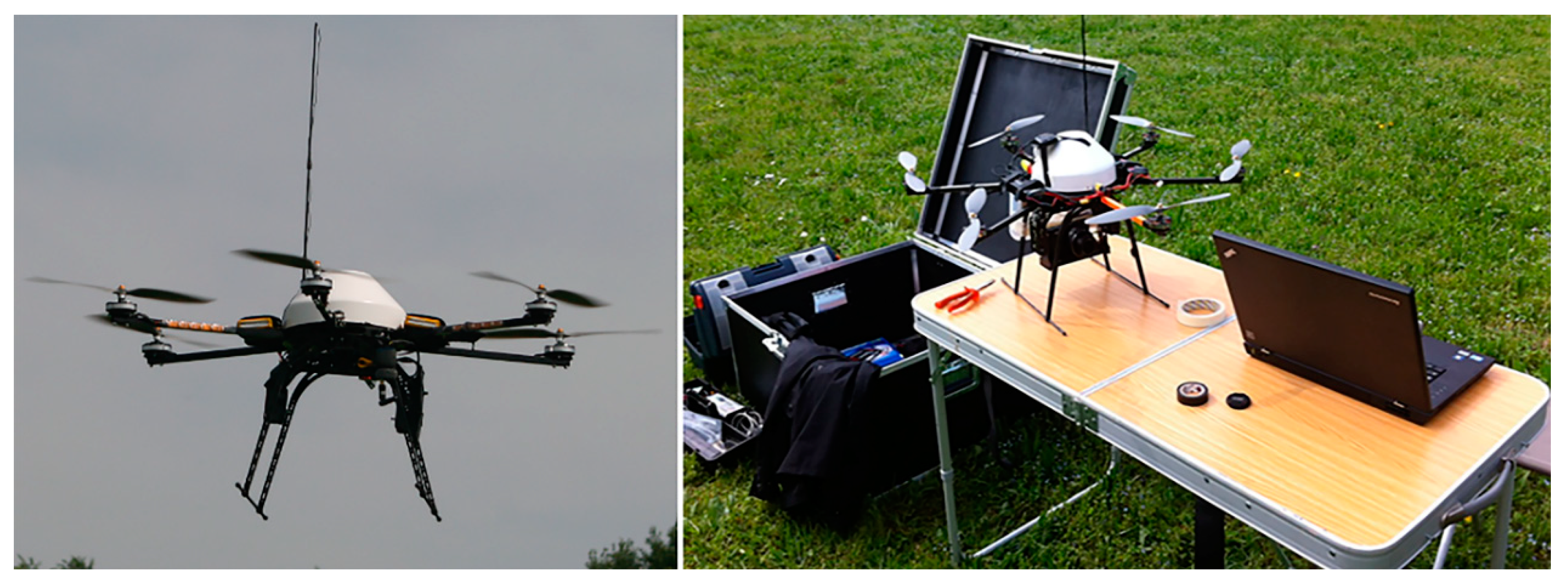
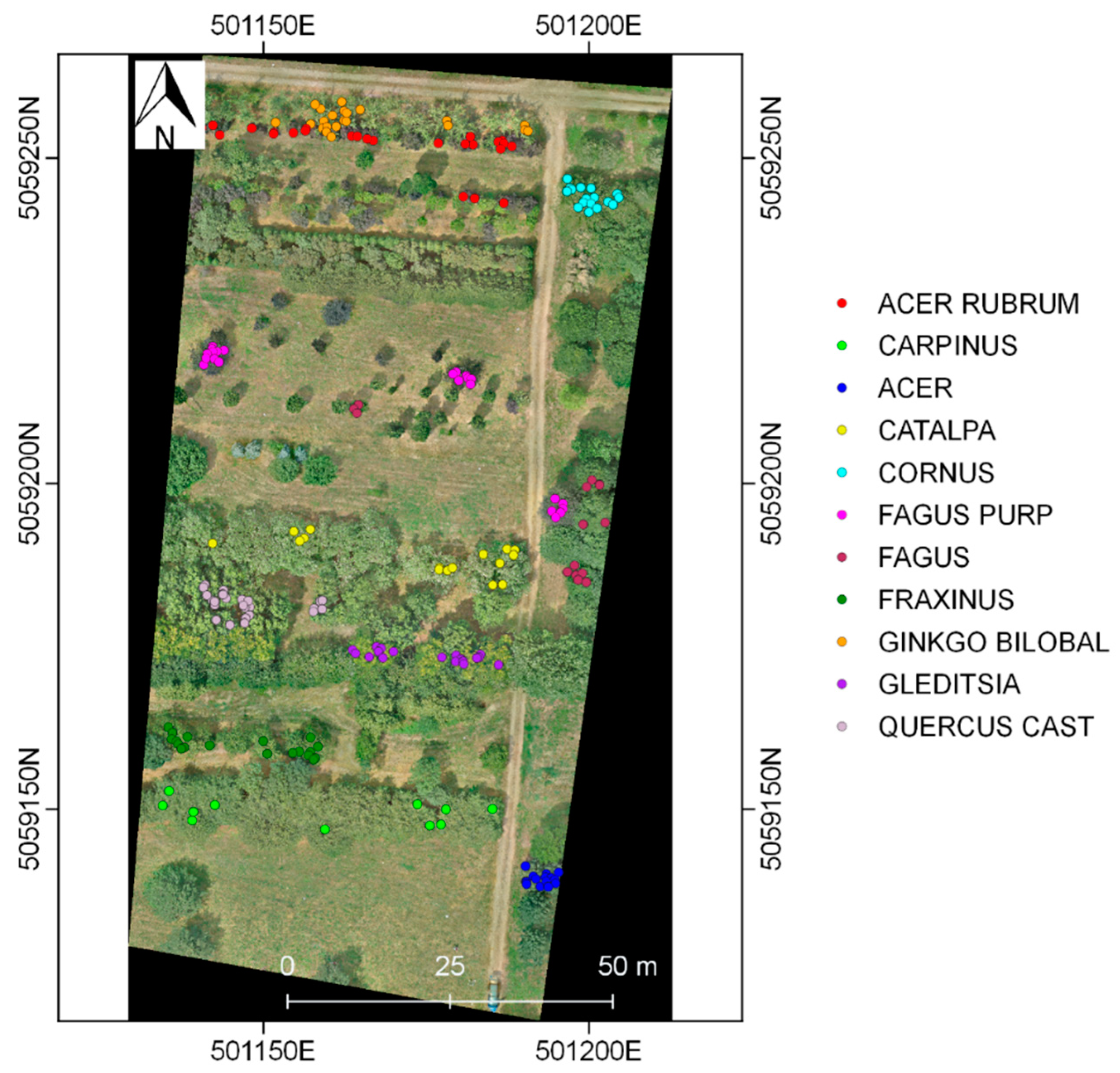
2 was selected inside a wide private plant nursery, close to Cirimido village, Como, Italy. This area was characterized by the presence of several tree species: maple (Acer spp.), red maple (Acer rubrum), hornbeam (Carpinus betulus), catalpa (Catalpa spp.), dogwood (Cornus spp.), beech (Fagus spp.), copper-beech (Fagus purpurea), ash (Fraxinus spp.), ginkgo biloba (Ginkgo biloba), honey locust (Gleditsia triacanthos), and chestnut-leaved oak (Quercus castaneifolia). The local technical staff provided information for their identification. The employed platform was the HexaKopter by the German company MikroKopter (Moormerland, Germany.), (Figure 2).
This powered vertical take-off and landing vehicle is equipped with six brushless motors; it weighs about 1.2 kg with batteries and its maximum transportable payload is equal to 0.5 kg. The HexaKopter can fly up to 200 m far from the take-off point and the flight duration is limited to 10 min.
Two different digital compact cameras were used for surveying. The Red Green Blue (RGB) digital compact camera was a mirrorless Nikon 1 J1 (Nikon Corporation, Tokyo, Japan). It weighs 310 g and acquires images in the visible part of the electromagnetic spectrum by means of a CMOS sensor of maximum size 10 Mpx. The other digital compact camera was a Tetracam ADC Lite (Tetracam Inc., Chatsworth, CA, USA): this lightweight (200 g) Agricultural Digital Camera (ADC) is specially designed for UAS applications and features a single CMOS sensor of 3.2 Mpx. The camera is optimized for capture of Green, Red and Near-Infrared (NIR) wavelengths approximately corresponding to Landsat TM2, TM3 and TM4 bands [25]. The resulting Color Infrared (CIR) imagery is suitable for derivation of several vegetation indices, canopy segmentation and band ratios. Further cameras details are reported in Table 1.

2.2. UAS Survey Planning and Data Collection

In summer, the multi-rotor HexaKopter was remotely piloted by an operator during landing and take-off, whilst a pre-set flight planning was used during the imagery acquisition. Owing to the UAV technical limitations, two separate flights were carried out, first with the Nikon 1 J1 and then with the Tetracam ADC Lite. To cover the entire area, it was necessary to plan the acquisition of four strips with forward and side overlaps equal to 85% and 50%, respectively. The flight plan was tuned according to the sensor with the lower geometric performance (i.e., the ADC Lite). Taking into account the various tree heights, the flight altitude was fixed at 40 m above ground level, thus producing different Ground Sample Distances (GSDs): 1.3 cm for the RGB images and 1.6 cm for the CIR ones. Thus, the Nikon 1 J1 acquired 125 images and the ADC Lite camera 159 CIR images.
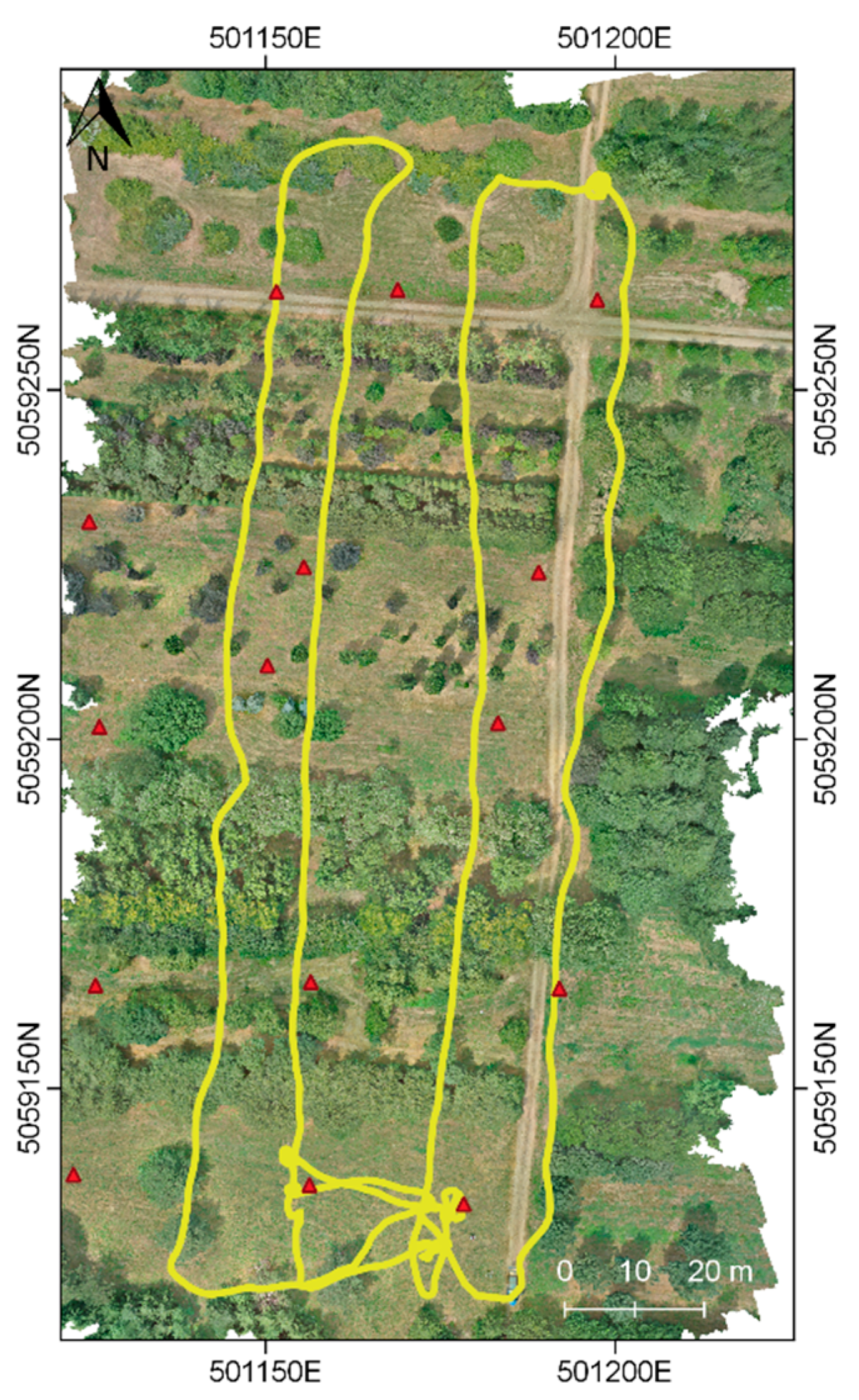
Fifteen black and white (b/w) square targets, with side of 30 cm and triangular pattern, were homogeneously distributed in the area. The center coordinates were measured by means of a GNSS receiver Trimble 5700 in NRTK (Network Real Time Kinematic) survey (Figure 3), with horizontal and vertical accuracies of 2–3 cm and 5 cm, respectively.
The geometric calibration of the cameras was performed, by taking some images of a b/w planar calibration grid of known geometric properties; the parameters of a Brown distortion model [26] were estimated through PhotoModeler Scanner [27]. Moreover, the CIR dataset was radiometrically corrected as recommended by the ADC Lite technical documentation [18]. Some images were taken of a small white Teflon calibration plate, provided with the camera, whose spectral response is known. These images were used by the accompanying software PixelWrench2 [28] to process all other images in relation to the sunlight during the acquisition period.
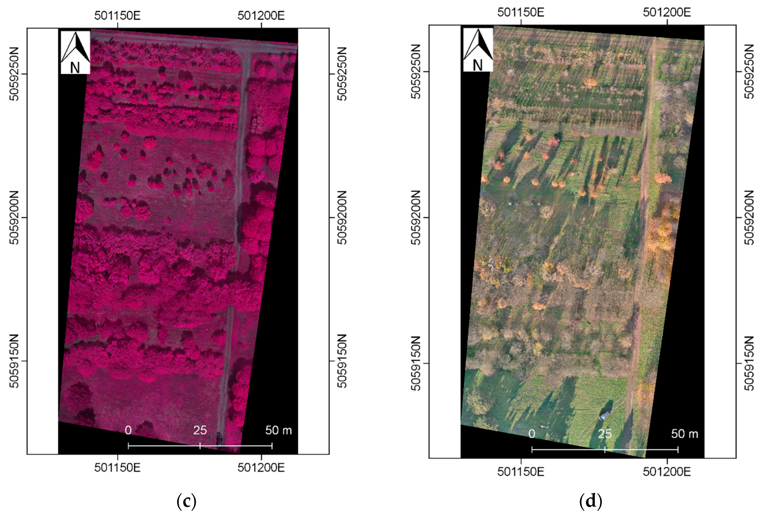
Aiming to make use of a multi-temporal dataset, after the first summer survey, a second one was planned in autumn, when some tree species are clearly recognizable thanks to their specific foliage color, as the red crowns of the copper-beech, or the yellow one of gingko. Unfortunately, due to a long period of bad weather conditions, the second survey took place at the end of November when some of tree species had already lost leaves. The same flight plan and a similar ground points survey were performed. Unique difference is that only the Nikon 1 J1 was employed, because the rainy weather forced to stop the survey prior to flying with the ADC Lite.
From here on, the three final datasets are identified with the names “RGB_S”, “CIR_S” and “RGB_A”, where “S” stands for summer and “A” for autumn.

2.3. Photogrammetric Processing

The Agisoft PhotoScan Professional software [29] was utilized to process the three image blocks, georeferenced on the 15 surveyed points [30]. Following the standard workflow proposed by the software, images were processed maintaining their full resolution (correspondent to the high alignment quality of the software), while the dense points clouds were generated downgrading the images with a factor equal to 4 (i.e., using the high quality of Agisoft Photoscan Pro). According to consolidate photogrammetric procedures, a Digital Surface Model (DSM) was generated with a mesh of 0.01 m by using the oriented RGB_S block, which has the full leaf coverage. RGB_S, RGB_A and CIR_S orthomosaics, with resolution equal to 0.01 m, were then produced through orthoprojection on the same DSM (Figure 4).
The georeferencing accuracies of the orthophotos were evaluated by means of the 14 surveyed ground points (one GPS surveyed point was eliminated due to gross errors). The Root Mean Square Errors (RMSE) on single coordinate of GCPs, reported in Table 2, are all lower than 5 cm, thus maintaining the global accuracy of the orthophotos consistent with the GPS survey accuracy.

2.4. Classification

To detect tree species, supervised classifications were performed using the Maximum Likelihood (ML) classifier. Reference data for the supervised classification were defined on orthophotos, making use of photographic and handwritten documentation gathered with the plant nursery staff. In detail, reference samples were selected in ENVI Classic V.5.1 [31], by digitizing polygons on the central part of tree crowns, to account for residual co-registration errors between orthophotos (Figure 5).
In order to represent the within-class variability, different individuals were used for each tree species. A standard approach [32] for selecting the samples was tested, with the aim to understand if Remote Sensing established methods are also suitable for UAS imagery or have to be fine-tuned in their respect. For each of the 11 considered tree classes, 30 polygons, with size equal to 5 × 4 pixels, were selected, for a total of 600 pixels. Lastly, the so-collected samples were randomly subdivided: a half was used as training samples to train the classification algorithm, the other half as validation samples to validate classification results. The quality of classification outputs was assessed through the Error Matrix (EM), by calculating the Overall Accuracy (OA), the Producer’s Accuracy (PA), the User’s Accuracy (UA), and the Kappa coefficient [33].

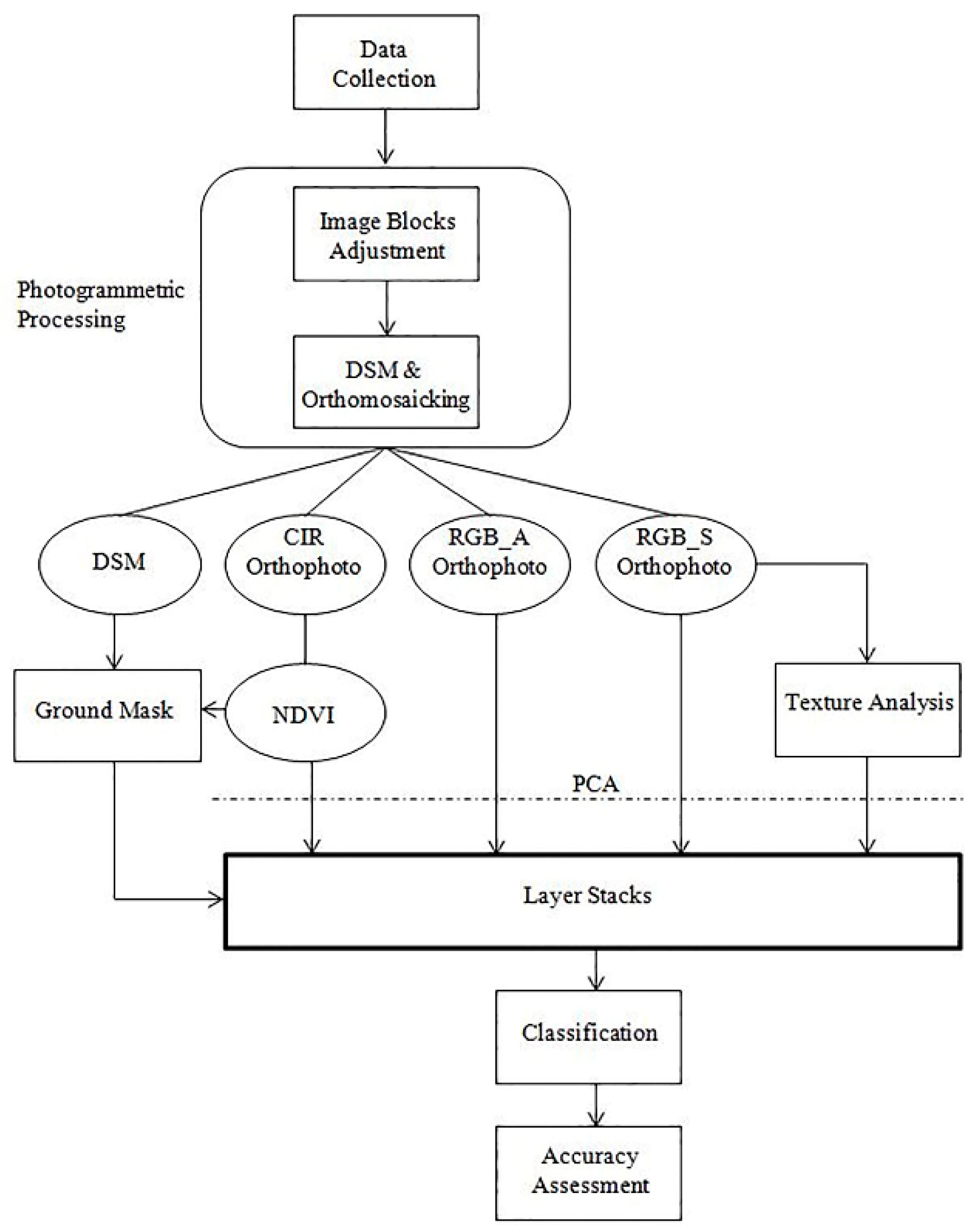
2.5. Processing of Multispectral Orthophotos

Some derived variables were computed from the 6 original layers acquired in summer (RGB_S and CIR_S). The first computed band was the Normalized Difference Vegetation Index (NDVI): this index is quite powerful in performing a qualitative classification thanks to the capability to distinguish alive vegetated areas from other surface types (water, soil, etc.). Successfully employed in hundreds of studies, it is expressed as the difference between the NIR and the Red bands (both from the CIR dataset) normalized by the sum of these [34]:
N D V I = N I R R E D N I R + R E D
As already explained in Section 2.2., CIR dataset was processed using a Teflon calibration target in order to perform spectral balance. Hence, the resulting NDVI is refined in relation to that day’s lighting conditions.
Then, texture measures were generated from spatial relationship of pixels. According to Gonzalez and Woods [35], texture can be defined as the measures of smoothness, coarseness, and regularity of an image region, and can be discriminated by using structural or statistical techniques. The latter are most suitable for natural image scenes with rare re-occurring patterns [36]: therefore, the commonly used Grey Level Co-occurrence Matrix (GLCM) method, suggested by Haralick et al. [37], was employed in this case study. The GLCM describes the texture in a user-defined moving window, by looking at the spatial co-occurrence of the grey levels of the included pixels. The GLCM algorithm computes a matrix that accounts for the difference in grey values between two pixels at a time, called the reference pixel and the neighbor pixel. In this case study, the neighbor pixel was located, each time, one pixel above and to the right of the reference pixel: according to Murray et al. [38], this offset of (1,1) is the most commonly used.
The GLCM was calculated for 24 different window sizes, ranging from the minimum value of 3 pixels to a maximum value of 49 pixels (corresponding to roughly 49 cm, i.e., included in most of tree crowns). Lastly, the GLCM implementation of ENVI provides the so-called eight standard Haralick measures, which can be subdivided into three categories [39]:
  • contrast based: contrast, dissimilarity, and homogeneity;
  • orderliness based: angular second moment and entropy;
  • statistically based: mean, variance, and correlation.
The GLCM calculations were performed only on one channel, to reduce data redundancy. Following the approach of Dorigo et al. [
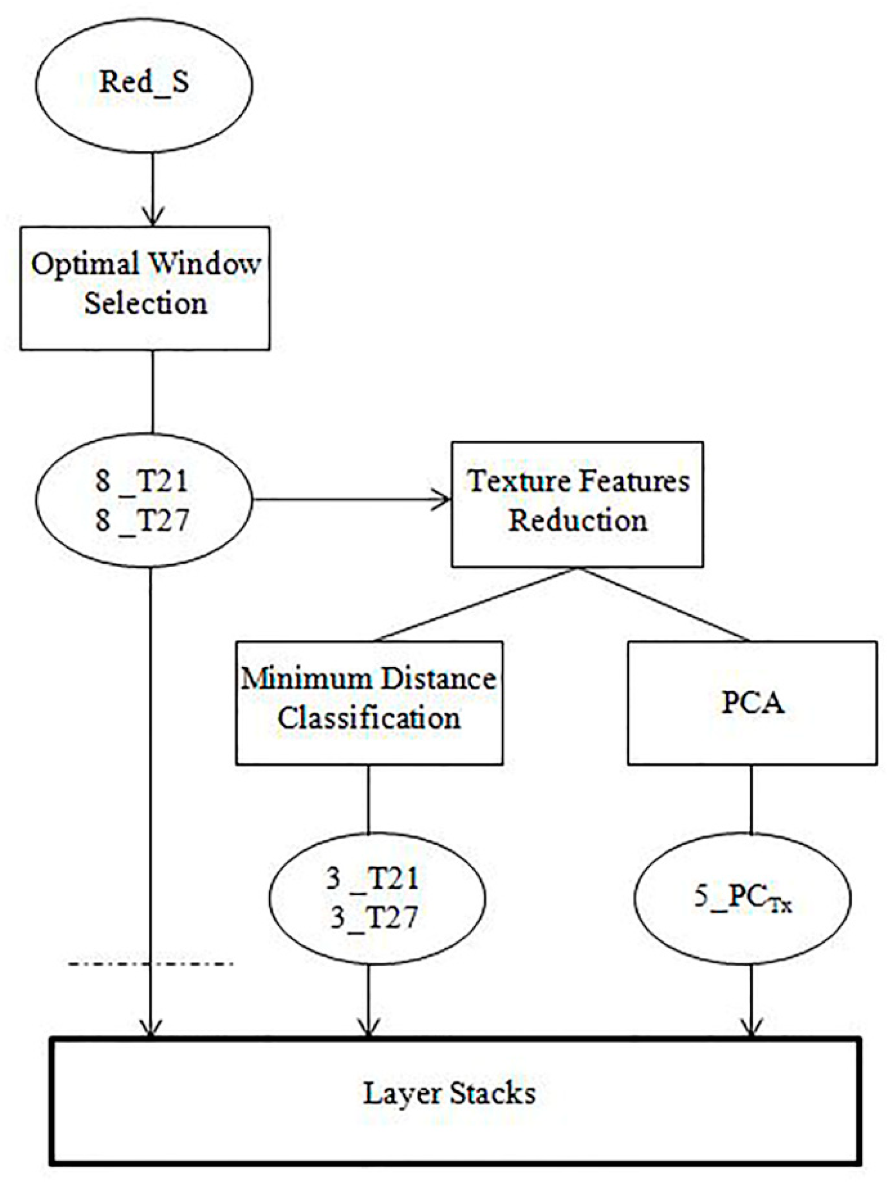
40], the band with the highest value of entropy was chosen; i.e., the Red summer band (Red_S). To summarize, for each window size (24, from 3 to 49 size) the 8 texture features were computed, on the Red_S band, with equal offset of (1,1). Then, a selection of the optimal window size was performed, as described below.
The final result of a texture analysis relies heavily on the adopted window size which, in turn, depends on several factors [41]. If the window is too small, then it does not contain enough information about the area; on the contrary, if the window is too large, it can overlap with other types of ground cover, thus producing erroneous results (the so-called edge effect [20]). However, despite the issue being recognized, a general method for establishing the optimum size has not yet been proposed. In this study, hence, two methods, usually applied to Remote Sensing standard imagery, were compared and used to determine the optimal window size.
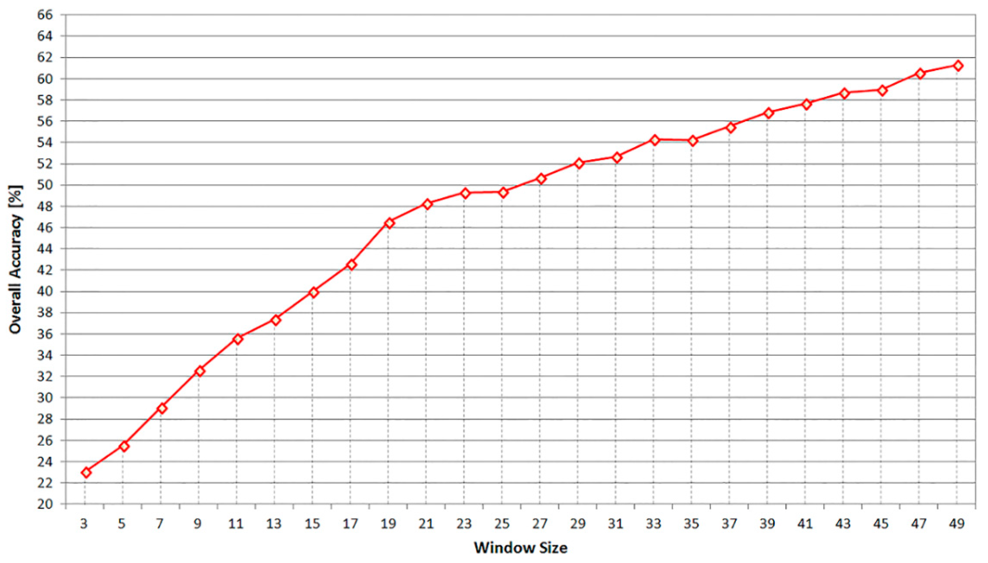
The first method performs the classification of all the computed texture features, for each window size, with the Maximum Likelihood classifier, as already done by Murray et al. [38], evaluating the behavior of classification accuracies. For each of the 24 different window sizes, the eight texture features were classified together with the Maximum Likelihood algorithm on training samples described in 2.4. By analyzing the Overall Accuracy provided by the Error Matrix [33], it was possible to observe how the accuracy varied with respect to the window size: as visible in Figure 6, classification accuracy grows with increasing window size.
Although it seems sensible to choose the largest window size, the optimal one is a compromise between having a good OA and minimizing the aforementioned edge effects. According to Murray et al. [38], the optimal window size corresponds to where the slope of accuracy curve varies. In this case, the slope value is 1.3 for window size from 0 to 19, 0.3 from 21 to 27 and 0.5 after 27. Hence, the main changes are in correspondence of values between 21 and 27, as shown in Figure 6.
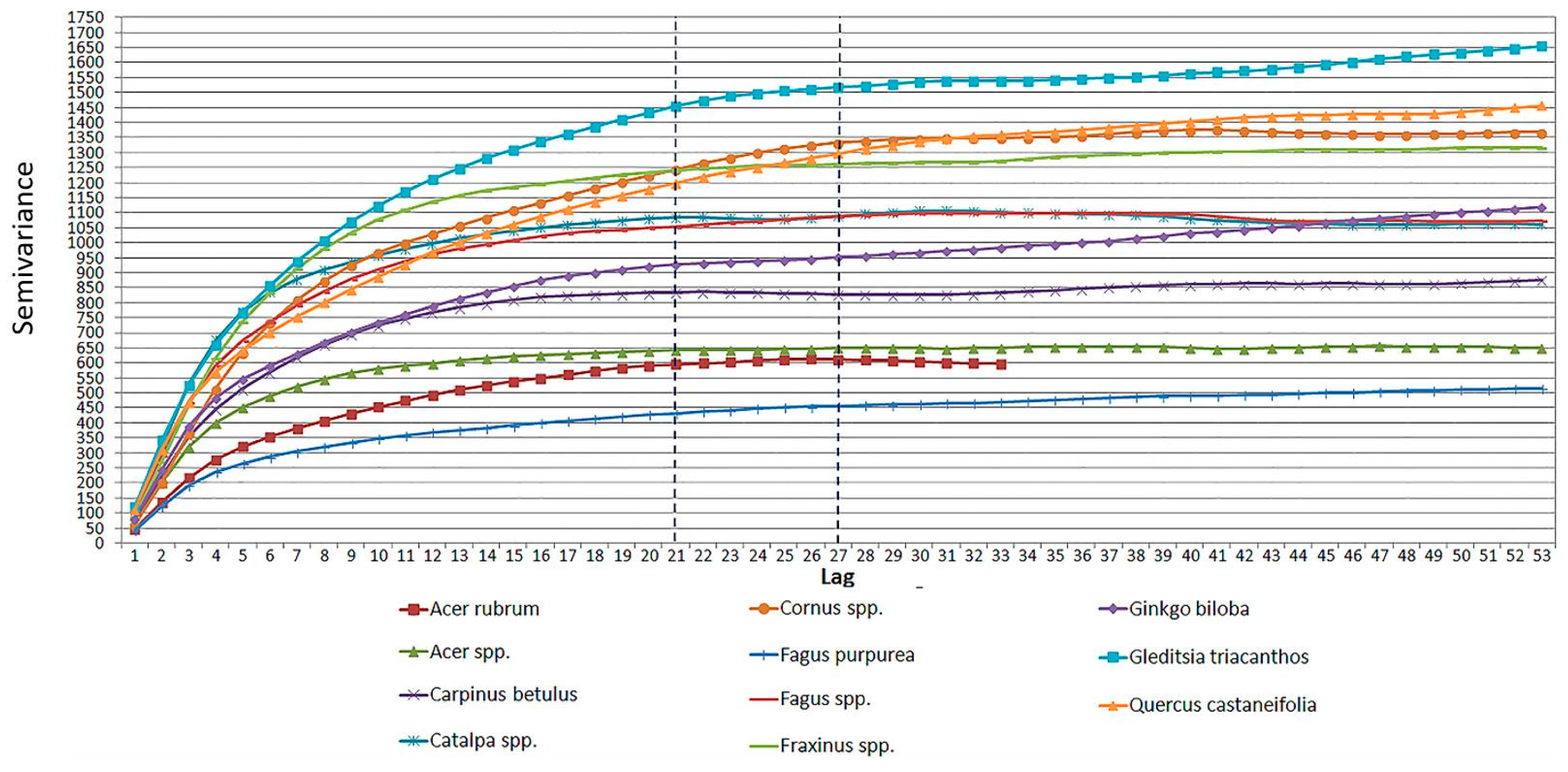
The second method, instead, is based on the empirical semivariance computation, which is a measure of data variations in the spatial domain [42]. The empirical semivariance γ(h) of a random function Z(x) is defined as
γ ( h ) = 1 2 N ( h ) i = 1 N ( h ) [ Z ( x i ) Z ( x i + h ) ] 2
where Z(xi) and Z(xi + h) are two values of the same function Z(x) at a distance h (lag); N is the total number of pairs at given lag h. For digital images; i.e., for digital functions in two dimensions—the optimal window size to describe a specific kind of coverage is the lag (range) that results in the maximum variability (sill) of a scene structure [43]. This method was applied on a sample set of pixels, selected on the Red_S channel, for each tree species. The related semivariograms are shown in Figure 7. The empirical semivariograms were best-fitted with exponential model. The resulting ranges, evaluated at a lag of 4 times the exponential constant, varied for the different tree species from a minimum of 18 to a maximum of 35. Four species have ranges close to 21, other four around 28, the remaining three saturate at higher lag. To avoid the use of too many layers in classification processing, only two representative values of window sizes were selected, and the two values determined with the previous method were chosen.
Therefore, both texture images produced with window sizes of 21 and 27 (called T21 and T27 from now on) were selected to be further analyzed.

2.6. Features Reduction

At this point, the available texture variables were the 8 Haralick features for each selected window size (21 and 27), for a total of 16, some of them strongly correlated: a reduction was therefore attempted. To this aim, two alternative procedures have been tested to select the optimal subset of features to be classified: a pre-classification of texture features with Minimum Distance algorithm, and a Principal Component Analysis (PCA), on texture or on all available bands (see Figure 8).

2.6.1. Minimum Distance Classification

According to Hall-Beyer [44], since texture features are highly correlated, only one from each texture category (contrast, order, statistical) should be used. In the first procedure each feature of T21 and T27 was classified individually by means of the Minimum Distance algorithm (unlike Maximum Likelihood, this algorithm is able to classify individual bands). Then, the OA provided by the Error Matrix was used to determine the best feature from each category (Table 3).
Concerning the texture image with the smaller window (21), the highest OA values correspond to Mean, Dissimilarity, and Entropy (3_T21). Instead, Mean, Homogeneity and Second Moment were chosen for the texture image with kernel size of 27 (3_T27).

2.6.2. Principal Component Analysis

The second features reduction strategy adopted was the PCA [45], through which the original data set is transformed into a new set of uncorrelated variables. The choice of the most significant components is made analyzing their variances (i.e., the eigenvalues of the covariance or correlation matrix) of the PCs with different strategies, as the Kaiser’s rule [46] or the Scree graph criterion [47]. The first method suggests that only components with variance bigger than 1 contain significant information and should be selected. The second criterion instead involves looking at the plot of the eigenvalues against the components number (Scree graph). The minimum number of meaningful components corresponds to the point where the slope of the curve suddenly decreases.
In this work the PCA was carried out on two different datasets with two different purposes:
  • on the 16 texture features only, as a texture reduction method;
  • on all the 20 available bands (RGB_S + NDVI + 16 texture features), as a general reduction method.
Since the values of the bands forming the datasets were not homogenous, PCA was based on the correlation matrix instead of the covariance one. In addition, the number of components to be retained was chosen by following the Scree graph criterion. The results of the first analysis on the 16 texture features, 8 deriving from window size T21 and 8 from window size T27, are shown in Table 4: components, eigenvalues and percentage of the variance with respect to the total variance are reported. The Scree graph is presented in Figure 9. According to this graph, five principal components were selected (5_PCTx).
The second application of the PCA was performed on a dataset of 20 bands, including 3 channels from RGB_S, the NDVI and 16 texture features (8_T21 + 8_T27). In Table 5 all the outcomes of this analysis are reported, whereas Figure 10 shows the Scree graph. Checking the graph, the major slope variations are in correspondence of component number 7 and 10. Since a subjective decision is necessary in this case, ten principal components were chosen, in order to have the same number of bands obtained combining the multispectral dataset (RGB_S + NDVI) and the 6 texture features of Section 2.6.1. (3_T21 + 3_T27) and compare classification results.

2.7. Masking the Ground

Before performing layer classifications, it was decided to mask out the ground (bare soil and grass coverage) by using information from DSM and NDVI, to avoid misclassifications between grass and tree species.
A masking layer was therefore computed through the concurrent use of DSM and NDVI: since the ground was almost flat, the zero value of the mask was assigned to DSM pixels with value lower or equal to the ground mean height (319 m) and to NDVI pixels with value lower or equal to 0.5. This mask was then applied to all layer stacks before being classified (Figure 11).

3. Results and Discussion

In the end, the following bands were available:
  • 9 original channels, from the RGB_S, CIR_S and RGB_A orthophotos;
  • 1 vegetation index, the NDVI;
  • 16 texture features, obtained with two different window sizes (8_T21 + 8_T27);
  • 6 texture features, from texture features reduction with Minimum Distance algorithm (3_T21 + 3_T27);
  • 5 PCs, deriving from texture features reduction with PCA (5_PCTx);
  • 10 PCs, from the PCA performed on the whole 20 variables.
Starting from these bands, different layer stacks were generated and classified:
  • The first layer stack is the simplest, being composed of the RGB_S orthophoto and the NDVI (4 bands);
  • The second layer stack is a multi-temporal dataset, with the RGB_A orthophoto added to the previous layer stack (7 bands);
  • In the third layer stack, all the 16 texture features were aggregated to the first layer stack, without considering any reduction (20 bands);
  • The fourth layer stack was obtained by adding the six best texture features identified through Minimum Distance classifier (see Section 2.6.1.) to the first layer stack (10 bands);
  • The fifth layer stack was created by adding to the first layer stack the 5 PCs selected from the 16 original texture variables (see Section 2.6.2.) (9 bands);
  • The last layer stack is composed by the 10 PCs extracted from the whole 20 variables (see Section 2.6.2.) (10 bands).
The Overall accuracy and the Kappa coefficient of the classification computed on all layer stacks are summarized in Table 6, whereas Table 7 shows the Producer’s and User’s Accuracies (PA and UA, respectively) of the most significant layer stacks: the first one is the simplest, without texture variables, the third and the sixth stack yield the highest values of OA and K, with texture and PCA feature reduction. Figure 12 reports the results for the classification computed on the aforementioned layer stacks.
It is possible to note in Table 6 that the first layer stack (RGB_S + NDVI) is characterized by a moderately low value of OA, as expected. It is used as benchmark for evaluating the other classification results. The OA increase (+13%) of the second layer stack (RGB_S + RGB_A + NDVI) proves the effectiveness of using a multi-temporal analysis: this obviously means that two or more UAS surveys are necessary at different times, chosen according to specific phenological characteristics of the tree species under study.
On the other hand, the concurrent employment of texture features and multispectral images leads to improvements in OA in the range of +19% and +30%, even without the use of multi-temporal data. Maximum values of OA and Kappa coefficient are reached by using all the eight texture measures for the two selected window sizes (third layer stack), but this implies the use of correlated bands. Significant improvements in classification accuracies, with respect to the first simple stack, but with a reduced number of layers (9 or 10) are obtained also applying different strategies of variables reduction: the methods used for bands selection (see Section 2.6.) yield very similar results in terms of accuracy, with OA ranging from 77.07% to 78.54%. Specifically, the fourth layer stack entails a more rigorous but time-consuming procedure, whilst the use of PCA is a well-known standard technique, implemented in image analysis software packages. PCA was applied only on texture features (fifth layer stack) or on all the available bands (sixth layer stack), reaching comparable classification results. As a matter of fact, the employment of PCA on all the 20 variables is preferable, as ensures to reduce possible correlation even among multispectral data.
By analyzing in detail the UA and PA of different tree species of the three most significant cases, the improvement introduced by the use of texture features is evident (Table 7), though depending on the species. The lowest increases (+6% or +10%) are observed for species that were well detected even with the simplest layer stack, only composed by radiometric information. Because of their peculiar radiometry, some tree species, such as Acer rubrum or Fagus purpurea, can be well distinguished from the other species, even without adding texture measures. Instead, the highest improvements are reached for species with low values of PA and UA in the first stack, which were confused with other tree species. In this case, the accuracies increase from a minimum of +32% (PA of Fraxinus spp.) to higher values of +68% and +75% (PA of Quercus castaneifolia.). For tree species similar in terms of radiometry, texture features become a determinant for their discrimination.

4. Conclusions

This study investigated whether the use of texture features, derived from ultra-high resolution UAS imagery, can improve the accuracy of vegetation classification. In this paper a workflow based on Remote Sensing standard methods was experimented.
Three UAS surveys were performed to acquire RGB and CIR imagery in summer and autumn and produce DSM and multispectral orthophotos. Synthetic bands were derived from the original layers and the Grey Level Co-occurrence Matrix was used to generate texture images. The methods usually applied to Remote Sensing standard imagery to select optimal features and optimal window size turned out to be suitable, despite the big differences in spatial resolution between satellite and UAS imagery.
Several and similar tree species can be well-detected by the described procedures. The classification tests proved that the addition of texture features improved the Overall Accuracy values, as well as the User’s and Producer’s Accuracies. Some tree species that were confused with others in the classification based on pure radiometric bands were better identified by introducing texture measures. Finally, in those case when multi-temporal surveys are not possible, tree species classification can be performed efficiently with single season survey, by means of texture features.
Nevertheless, the use of texture variables in ultra-high resolution imagery classification still needs to be assessed. The lack of a well-established methodology can be attributed to a number of factors, including the strong dependence of texture measures upon image characteristics (e.g., image scale, the number of spectral bands, image context and class definition) as well as the absence of an a priori approach for texture selection, as outlined also by Kelcey and Lucieer [2]. In order to robustly address these issues, further tests should be therefore carried out.

Author Contributions

Conceptualization, R.G. and G.S.; Data curation, R.G. and D.P.; Methodology, R.G., G. S. and G.R.; Supervision, G.S. and L.P.; Validation, R.G., G.S. and G.R.; Writing—original draft, R.G., G.S. and G.R.; Writing—review & editing, G.S. and L.P.

Funding

This research received no external funding.

Acknowledgments

The authors wish to thank the plant nursery “Peverelli S.R.L.” and its staff for the shown availability. The instrumentation used in this study is owned by the Geomatics and Geodesy Section of the Department of Civil and Environmental Engineering at Politecnico di Milano.

Conflicts of Interest

The authors declare no conflict of interest.

References

  1. Colomina, I.; Molina, P. Unmanned Aerial Systems for Photogrammetry and Remote Sensing: A review. ISPRS J. Photogramm. Remote Sens. 2014, 92, 79–97. [Google Scholar] [CrossRef]
  2. Dunford, R.; Michel, K.; Gagnage, M.; Piegay, H.; Trémelo, M.L. Potential and constraints of Unmanned Aerial Vehicle technology for the characterization of Mediterranean riparian forest. Int. J. Remote Sens. 2009, 30, 4915–4935. [Google Scholar] [CrossRef]
  3. Kelcey, J.; Lucieer, A. An adaptive texture selection framework for ultra-high resolution UAV imagery. In Proceedings of the IEEE International Geoscience and Remote Sensing Symposium (IGARSS), Melbourne, Australia, 21–26 July 2013; pp. 3883–3886. [Google Scholar] [CrossRef]
  4. DeBell, L.; Anderson, K.; Brazier, R.E.; King, N.; Jones, L. Water resource management at catchment scales using lightweight UAVs: Current capabilities and future perspectives. J. Unmanned Veh. Syst. 2015, 4, 7–30. [Google Scholar] [CrossRef]
  5. Peng, Z.R.; Wang, D.; Wang, Z.; Gao, Y.; Lu, S. A study of vertical distribution patterns of PM2.5 concentrations based on ambient monitoring with Unmanned Aerial Vehicles: A case in Hangzhou, China. Atmos. Environ. 2015, 123, 357–369. [Google Scholar] [CrossRef]
  6. Gonzalez, L.F.; Montes, G.A.; Puig, E.; Johnson, S.; Mengersen, K.; Gaston, K.J. Unmanned Aerial Vehicles (UAVs) and Artificial Intelligence Revolutionizing Wildlife Monitoring and Conservation. Sensors 2016, 16, 97. [Google Scholar] [CrossRef] [PubMed] [Green Version]
  7. Zhang, Q.; Qin, R.; Huang, X.; Fang, Y.; Liu, L. Classification of ultra-high resolution orthophotos combined with DSM using a dual morphological top hat profile. Remote Sens. 2015, 7, 16422–16440. [Google Scholar] [CrossRef]
  8. Rango, A.; Laliberte, A.S.; Herrick, J.E.; Winters, C.; Havstad, K.; Steele, C.; Browning, D. Unmanned aerial vehicle-based Remote Sensing for rangeland assessment, monitoring, and management. J. Appl. Remote Sens. 2009, 3, 1–15. [Google Scholar] [CrossRef]
  9. Laliberte, A.S.; Goforth, M.A.; Steele, C.M.; Rango, A. Multispectral Remote Sensing from Unmanned Aircraft: Image processing workflows and applications for rangeland environment. Remote Sens. 2011, 3, 2529–2551. [Google Scholar] [CrossRef]
  10. Lucieer, A.; Robinson, S.; Turner, D.; Harwin, S.; Kelcey, J. Using a micro-UAV for ultra-high resolution multi-sensor observations of Antarctic moss beds. In Proceedings of the 2012 XXII ISPRS Congress, Melbourne, Australia, 25 August–1 September 2012; Volume 39/B1, pp. 429–433. [Google Scholar] [CrossRef]
  11. Turner, D.; Lucieer, A.; Malenovský, Z.; King, D.H.; Robinson, S.A. Spatial co-registration of ultra-high resolution visible, multispectral and thermal images acquired with a micro-UAV over Antarctic moss beds. Remote Sens. 2014, 6, 4003–4024. [Google Scholar] [CrossRef]
  12. Goktogan, A.H.; Sukkarieh, S.; Bryson, M.; Randle, J.; Lupton, T.; Hung, C. A rotary-wing unmanned air vehicle for aquatic weed surveillance and management. J. Intell. Robot. Syst. 2010, 57, 467–484. [Google Scholar] [CrossRef]
  13. Hardin, P.J.; Jackson, M.W.; Anderson, V.J.; Johnson, R. Detecting Squarrose Knapweed (Centaurea virgata Lam. Ssp. squarrosa Gugl.) using a Remotely Piloted Vehicle: A Utah case study. GIsci. Remote Sens. 2007, 44, 203–219. [Google Scholar] [CrossRef]
  14. Gini, R.; Passoni, D.; Pinto, L.; Sona, G. Use of Unmanned Aerial Systems for multispectral survey and tree classification: A test in a park area of northern Italy. Eur. J. Remote Sens. 2014, 47, 251–269. [Google Scholar] [CrossRef]
  15. Baena, S.; Moat, J.; Whaley, O.; Boyd, D.S. Identifying species from the air: UAVs and the very high resolution challenge for plant conservation. PLoS ONE 2017, 12, e0188714. [Google Scholar] [CrossRef] [PubMed]
  16. Stroppiana, D.; Villa, P.; Sona, G.; Ronchetti, G.; Candiani, G.; Pepe, M.; Busetto, L.; Migliazzi, M.; Boschetti, M. Early season weed mapping in rice crops using multi-spectral UAV data. Int. J. Remote Sens. 2018, 1–21. [Google Scholar] [CrossRef]
  17. David, L.C.G.; Ballado, A.H. Vegetation indices and textures in object-based weed detection from UAV imagery. In Proceedings of the 6th IEEE International Conference on Control System, Computing and Engineering, Penang, Malaysia, 25–27 November 2016; pp. 273–278. [Google Scholar] [CrossRef]
  18. Tamouridou, A.A.; Alexandridis, T.K.; Pantazi, X.E.; Lagopodi, A.L.; Kashefi, J.; Moshou, D. Evaluation of UAV imagery for mapping Silybum marianum weed patches. Int. J. Remote Sens. 2017, 38, 2246–2259. [Google Scholar] [CrossRef]
  19. Liu, T.; Li, R.; Zhong, X.; Jiang, M.; Jin, X.; Zhou, P.; Liu, S.; Sun, C.; Guo, W. Estimates of rice lodging using indices derived from UAV visible and thermal infrared images. Agric. For. Meteorol. 2018, 252, 144–154. [Google Scholar] [CrossRef]
  20. Coburn, C.A.; Roberts, A.C. A multiscale texture analysis procedure for improved forest stand classification. Int. J. Remote Sens. 2004, 25, 4287–4308. [Google Scholar] [CrossRef] [Green Version]
  21. Rodriguez-Galiano, V.F.; Chica-Olmo, M.; Abarca-Hernandez, F.; Atkinson, P.M.; Jeganathan, C. Random Forest classification of Mediterranean land cover using multi-seasonal imagery and multi-seasonal texture. Remote Sens. Environ. 2012, 121, 93–107. [Google Scholar] [CrossRef]
  22. Laliberte, A.S.; Rango, A. Texture and scale in object-based analysis of subdecimeter resolution unmanned aerial vehicle (UAV) imagery. IEEE Trans. Geosci. Remote Sens. 2009, 47, 761–770. [Google Scholar] [CrossRef]
  23. Feng, Q.; Liu, J.; Gong, J. UAV Remote Sensing for Urban Vegetation Mapping Using Random Forest and Texture Analysis. Remote Sens. 2015, 7, 1074–1094. [Google Scholar] [CrossRef] [Green Version]
  24. Alvarez-Taboada, F.; Paredes, C.; Julián-Pelaz, J. Mapping of the Invasive Species Hakea sericea Using Unmanned Aerial Vehicle (UAV) and WorldView-2 Imagery and an Object-Oriented Approach. Remote Sens. 2017, 9, 913. [Google Scholar] [CrossRef]
  25. Tetracam Inc. Agricultural Digital Camera User’s Guide; Version 2.3; Tetracam Inc.: Chatsworth, CA, USA, 2011. [Google Scholar]
  26. Brown, D.C. Close-Range Camera Calibration. Photogramm. Eng. 1971, 37, 855–866. [Google Scholar]
  27. PhotoModeler Scanner V.7.2012.2.1, by Eos System Inc. Available online: http://www.photomodeler.com/index.html (accessed on 16 February 2015).
  28. PixelWrench2, by Tetracam Inc. Available online: http://www.tetracam.com/Products_PixelWrench2.html (accessed on 16 February 2015).
  29. Agisoft PhotoScan Professional, V.0.9.0. Available online: http://www.agisoft.com/ (accessed on 16 February 2015).
  30. Sona, G.; Pinto, L.; Pagliari, D.; Passoni, D.; Gini, R. Experimental analysis of different software packages for orientation and digital surface modelling from UAV images. Earth Sci. Inf. 2014, 7, 97–107. [Google Scholar] [CrossRef]
  31. ENVI Classic V.5.1, by Harris. Available online: http://www.harrisgeospatial.com/ProductsandSolutions/GeospatialProducts/ENVI.aspx (accessed on 17 May 2017).
  32. Brivio, P.A.; Lechi, G.; Zilioli, E. Principi e Metodi di Telerilevamento. CittáStudi Edizioni; Utet: Torino, Italy, 2006; ISBN 88-251-7293-1. [Google Scholar]
  33. Congalton, R.G.; Green, K. Assessing the Accuracy of Remotely Sensed Data: Principles and Practices, 2nd ed.; Taylor & Francis Group: Boca Raton, FL, USA, 2008. [Google Scholar]
  34. Rouse, J.W., Jr.; Haas, R.H.; Schell, J.A.; Deering, D.W. Monitoring Vegetation System in the Great Plains with ERTS. In Proceedings of the Third Earth Resources Technology Satellite-1 Symposium, Greenbelt, MD, USA, 10–14 December 1974; pp. 309–317. [Google Scholar]
  35. Gonzalez, R.C.; Woods, R.E. Digital Image Processing; Addison-Wesley Publishing Company: Boston, MA, USA, 1992. [Google Scholar]
  36. Nalwa, V.S. A Guided Tour of Computer Vision; Addison-Wesley Publishing Company: Boston, MA, USA, 1993. [Google Scholar]
  37. Haralick, R.M.; Shanmugam, K.; Dinstein, I. Textural features for image classification. IEEE Trans. Syst. Man Cybern. 1973, 6, 610–621. [Google Scholar] [CrossRef]
  38. Murray, H.; Lucieer, A.; Williams, R. Texture-based classification of sub-Antarctic vegetation communities on Heard Island. Int. J. Appl. Earth Obs. Geoinf. 2010, 12, 138–149. [Google Scholar] [CrossRef]
  39. Nixon, M.S.; Aguado, A.S. Feature Extraction and Image Processing; Butterworth-Heinemann: Newnes, UK, 2002. [Google Scholar]
  40. Dorigo, W.; Lucieer, A.; Podobnikar, T.; Čarni, A. Mapping invasive Fallopia japonica by combined spectral, spatial, and temporal analysis of digital orthophotos. Int. J. Appl. Earth Obs. Geoinf. 2012, 19, 185–195. [Google Scholar] [CrossRef]
  41. Franklin, S.E.; Hall, R.J.; Moskal, L.M.; Maudie, A.J.; Lavigne, M.B. Incorporating texture into classification of forest species composition from airborne multispectral images. Int. J. Remote Sens. 2000, 21, 61–79. [Google Scholar] [CrossRef]
  42. Hay, G.J.; Niemann, K.O.; McLean, G.F. An object-specific image-texture analysis of H-resolution forest imagery. Remote Sens. Environ. 1996, 55, 108–122. [Google Scholar] [CrossRef]
  43. Tsai, F.; Chou, M.J. Texture augmented analysis of high resolution satellite imagery in detecting invasive plant species. J. Chin. Inst. Eng. 2006, 29, 581–592. [Google Scholar] [CrossRef]
  44. Hall-Beyer, M. GLCM Texture: A Tutorial, Version 2.10. 2007. Available online: http://www.fp.ucalgary.ca/mhallbey/tutorial.htm (accessed on 3 May 2016).
  45. Jolliffe, I.T. Principal Component Analysis, 2nd ed.; Springer: New York, NY, USA, 2002. [Google Scholar]
  46. Kaiser, H.F. The application of electronic computers to factor analysis. Educ. Psychol. Meas. 1960, 20, 141–151. [Google Scholar] [CrossRef]
  47. Cattell, R.B. The scree test for the number of factors. Multivar. Behav. Res. 1966, 1, 245–276. [Google Scholar] [CrossRef] [PubMed]
Figure 1. General workflow.
Ijgi 07 00315 g001
Figure 2. PoliMi HexaKopter with the Ground Control Station.
Ijgi 07 00315 g002
Figure 3. Flight tracks (yellow lines) for the RGB summer survey and positions (red triangles) of the 15 b/w targets for the GNSS survey.
Ijgi 07 00315 g003
Figure 4. Photogrammetric products: DSM (a) and orthomosaics: RGB_S (b), CIR_S (c) and RGB_A (d).
Ijgi 07 00315 g004aIjgi 07 00315 g004b
Figure 5. Centroids of the reference polygons used for classification purposes.
Ijgi 07 00315 g005
Figure 6. Overall Accuracies of the classifications of textures with different window sizes.
Ijgi 07 00315 g006
Figure 7. Tree species semivariograms.
Ijgi 07 00315 g007
Figure 8. Texture analysis workflow. 8_T21 and 8_T27 are the 8 texture variables available for each selected window size (21 and 27). 3_T21 and 3_T27 are 3 texture variables extracted from the 8 available for each selected window size (21 and 27) with a minimum distance classification. 5_PCTx are the variables resulting from the Principal Component Analysis (PCA) on the 8_T21 and 8_T27 together. The dotted line represents the PCA computed on all variables (RGB orthophotos, NDVI map and texture variables).
Ijgi 07 00315 g008
Figure 9. Scree graph of PCA on 16 texture features.
Ijgi 07 00315 g009
Figure 10. Scree graph of PCA on all the 20 bands.
Ijgi 07 00315 g010
Figure 11. The mask (left) and the masked RGB_S orthophoto (right).
Ijgi 07 00315 g011
Figure 12. Classification results for the first layer stack (a), the third layer stack (b) and the sixth layer stack (c).
Ijgi 07 00315 g012
Table 1. Technical specifications of the cameras.
Nikon 1 J1Tetracam ADC Lite
Focal length (mm)10.508.00
Sensor (mm)13.20 × 8.806.55 × 4.92
Sensor (px)3872 × 25922048 × 1536
Field of view (°)64.344.5
Pixel size (μm)3.403.20
Table 2. Statistics of the differences with respect to the surveyed ground points (m).
RMSETotal RMSE
EastNorthHeight
RGB_S-GNSS0.0220.0260.0270.044
CIR-GNSS0.0530.0370.0300.072
RGB_A-GNSS0.0490.0310.0430.072
Table 3. Overall Accuracies of the single features classified by the Minimum Distance algorithm (texture images with window size of 21 and 27).
CategoryFeatureOA (%)
Texture_21 × 21Texture_27 × 27
StatisticalMean21.7621.70
Variance15.9816.64
Correlation19.9819.50
ContrastHomogeneity19.4421.97
Contrast20.4319.35
Dissimilarity20.4620.31
OrderlinessEntropy19.2917.00
Second Moment18.4818.00
Table 4. Eigenvalues and variance percentage of PCA on 16 texture features.
ComponentEigenvalueVariance (%)
19.48859.300
22.60916.308
31.98312.392
41.1577.234
50.2401.498
60.1951.220
70.1080.675
80.0910.569
90.0450.282
100.0340.211
110.0140.089
120.0130.079
130.0100.063
140.0090.055
150.0030.020
160.0010.004
Table 5. Eigenvalues and variance percentage of PCA on the all 20 bands.
ComponentEigenvalueVariance (%)
19.90049.498
23.60518.024
32.55212.759
41.4057.024
50.9904.952
60.6413.204
70.2401.198
80.1950.975
90.1140.571
100.1070.535
110.0910.454
120.0450.224
130.0350.175
140.0330.167
150.0140.071
160.0120.062
170.0090.047
180.0080.039
190.0030.016
200.0010.003
Table 6. OA of different layer stacks, classified by the Maximum Likelihood algorithm.
IDLayer Stack# BandsOA (%)Kappa
1RGB_S + NDVI458.560.5442
2RGB_S + RGB_A + NDVI771.860.6905
3RGB_S + NDVI + 8_T21 + 8_T272087.180.8590
4RGB_S + NDVI + 3_T21 + 3_T271077.070.7478
5RGB_S + NDVI + 5_PCTx977.640.7540
6PCA(RGB_S + NDVI + 8_T21 + 8_T27)1078.540.7640
Table 7. Producer’s and User’s Accuracies of layer stacks number 1, 3 and 6.
Layer Stack #1 (4 Bands)Layer Stack #3 (20 Bands)Layer Stack #6 (10 Bands)
UA (%)PA (%)UA (%)PA (%)UA (%)PA (%)
Acer76.3191.1296.7497.7089.3997.04
Acer rubrum84.6275.9998.9492.4394.2285.86
Carpinus57.9566.6778.0089.2269.8982.68
Catalpa59.5241.5385.0870.1075.3848.84
Cornus53.6459.0074.0490.3368.7979.33
Fagus39.5451.5086.8881.4070.0770.76
Fagus purpurea78.0886.0993.2796.3687.5493.05
Fraxinus28.2431.8972.9385.0560.3066.11
Ginkgo biloba66.6770.0091.3287.6783.4485.67
Gleditsia52.8958.0093.1081.0078.0973.67
Quercus cast43.0212.1797.0887.5091.7680.59

