Point of Interest Matching between Different Geospatial Datasets


1
School of Resource and Environmental Science, Wuhan University, Wuhan 430079, China
2
Research Center of Government GIS, Chinese Academy of Surveying and Mapping, Beijing 100830, China
*
Author to whom correspondence should be addressed.
ISPRS Int. J. Geo-Inf. 2019, 8(10), 435; https://0-doi-org.brum.beds.ac.uk/10.3390/ijgi8100435
Submission received: 23 July 2019
/
Revised: 16 September 2019
/
Accepted: 29 September 2019
/
Published: 1 October 2019
(This article belongs to the Special Issue Information Fusion Based on GIS)
Abstract
:Point of interest (POI) matching finds POI pairs that refer to the same real-world entity, which is the core issue in geospatial data integration. To address the low accuracy of geospatial entity matching using a single feature attribute, this study proposes a method that combines the D–S (Dempster–Shafer) evidence theory and a multiattribute matching strategy. During POI data preprocessing, this method calculates the spatial similarity, name similarity, address similarity, and category similarity between pairs from different geospatial datasets, using the multiattribute matching strategy. The similarity calculation results of these four types of feature attributes were used as independent evidence to construct the basic probability distribution. A multiattribute model was separately constructed using the improved combination rule of the D–S evidence theory, and a series of decision thresholds were set to give the final entity matching results. We tested our method with a dataset containing Baidu POIs and Gaode POIs from Beijing. The results showed the following—(1) the multiattribute matching model based on improved DS evidence theory had good performance in terms of precision, recall, and F1 for entity-matching from different datasets; (2) among all models, the model combining the spatial, name, and category (SNC) attributes obtained the best performance in the POI entity matching process; and (3) the method could effectively address the low precision of entity matching using a single feature attribute.
1. Introduction
With the rapid development of ubiquitous cyberspace and internet information collection technologies, a large number of points of interest (POIs) [1,2] were aggregated into geospatial databases through social networks (such as Facebook, Flickr, and Sina Weibo) and map service providers (such as Open Street Map, Google Map, Baidu Map, and Gaode Map) [3]. Integrating multisource spatial data from the internet is a major challenge for current applications based on web-based information retrieval, spatial analysis, and spatial decision-making [4]. Geographic information collected from different sources often has inconsistencies, redundancy, ambiguity, and conflicts [5]; additionally, different platforms typically provide different description attributes for the same geospatial object. For example, Facebook usually provides check-in data [6], including location and text description information, while Flickr provides location and photo information [7]. Furthermore, the description attributes provided by the same platform for the same geospatial object might differ in terms of temporal precision, positional accuracy, and semantic precision [8]. Researchers and application developers often need to fuse the different attributes of POI data to obtain richer and more complete information about an object [9], update existing datasets or create new products [10,11]. Unfortunately, it is difficult to match the same object in different source datasets since there is no global identifier [9,12].
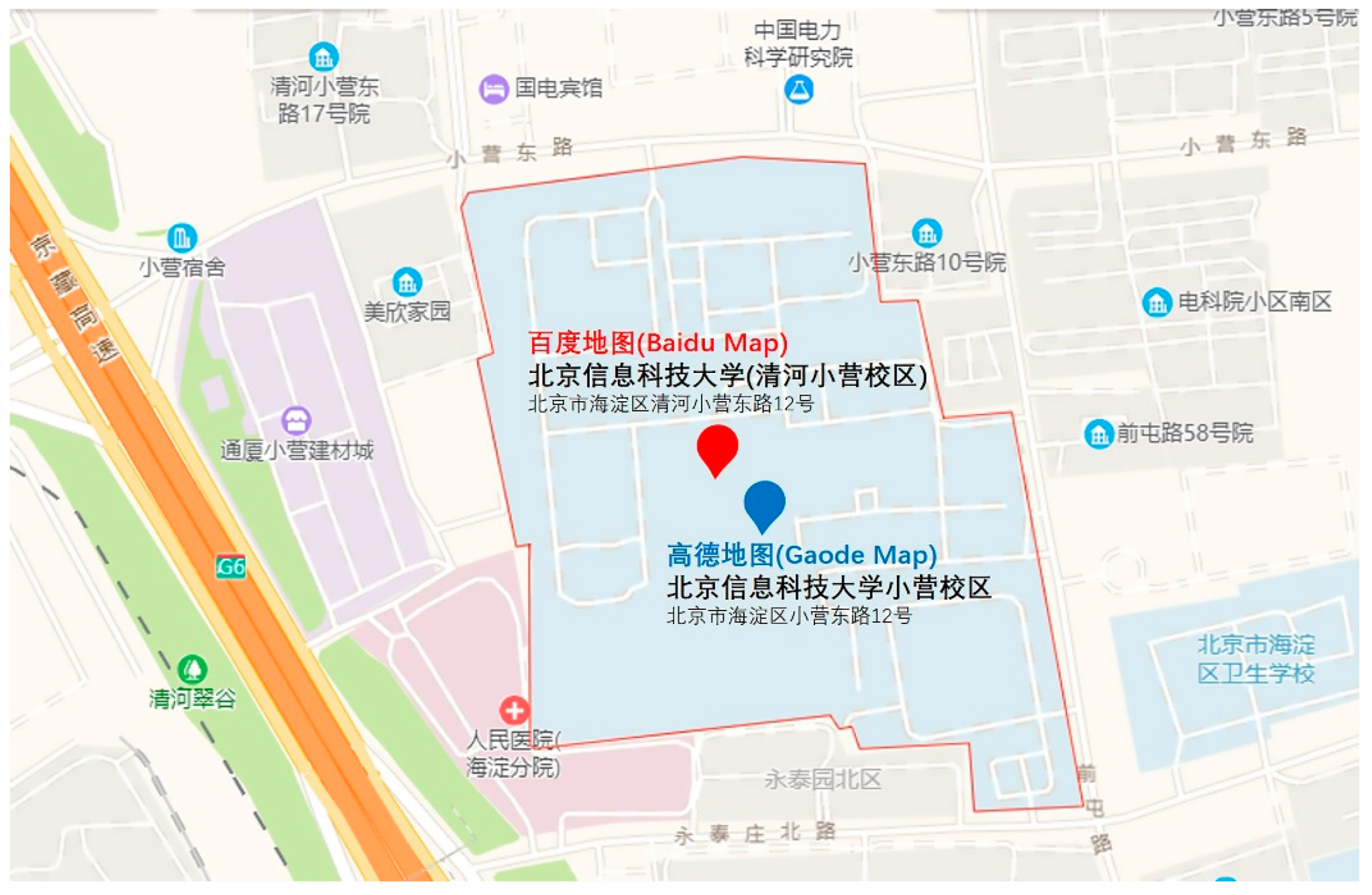
In general, data integration in geographic information systems (GISs) can be divided into two stages. First, matching is done to analyze the differences and similarities of spatial entities in different sources through a series of similar indicators, that is, to determine whether two objects from different datasets represent the same place in a geographical space [13]. An example is the geotag recommendation [14]. Weibo and Facebook allow users to add geographic locations while making posts. It can sometimes be difficult for a user to type these tags correctly. Therefore, to improve the user experience, we can use the space and text information of the post to find a similar geographical location in the Sina Weibo Map as a suggestion. Second, there is integration. Data integration involves combining the attributes of data from different sources and providing users with a unified and richer view of them [15]. To date, there is no standard way of integrating geospatial data from different sources, and manual integration can be very expensive. Of these steps, matching is the most crucial and difficult operation in data integration [16]. However, finding corresponding entities is difficult because geospatial data from different sources differs not only in data structure, content, focus, and coverage areas but also in semantic attributes (e.g., name, location, category) [17]. Figure 1 shows the differences in the name attribute, address attribute, spatial attribute, and category attribute for a pair of corresponding POI pairs obtained from the Baidu Map and the Gaode Map (both are well-known location-based service (LBS) applications). A POI record is represented by {source/name/address/spatial/category}.
POI 1 = {Baidu Map/Beijing Information Science and Technology University (Qinghe Xiaoying Campus) (北京信息科技大学(清河小营校区))/No. 12 Xiaoying East Road, Qinghe, Haidian District, Beijing (北京市海淀区清河小营东路12号)/40.04290645,116.3361188/education and training (教育培训)};
POI 2 = {Gaode Map/Beijing Information Science and Technology University Xiaoying Campus (北京信息科技大学小营校区)/No. 12 Xiaoying East Road, Haidian District, Beijing (北京市海淀区小营东路12号)/40.03842,116.339568/science and education cultural service (科教文化服务)}.
Here, the differences in spatial coordinates might be due to the nonlinear offset processing of data coordinates by different data providers for data security. The name is a spontaneous cognitive and socially situated linguistic concept, which inevitably results in word and semantic ambiguity [18]. In addition, abbreviations and whole words might refer to the same object; for example, both “US” and “United States” refer to the United States. Consequently, although many approaches have been proposed for matching geospatial entities from different sources, high-precision geospatial entity matching remains a major challenge.
In this paper, our work focuses on the first step in geospatial data integration—matching. Our goal is to find all pairs of POIs mentions between two different sources that refer to the same real-world entity. The remainder of this paper is organized as follows. Section 2 presents the related work. Section 3 presents the attributes of each geographic entity and their similarity measures and then describes the multiattribute matching method based on the Dempster–Shafer (D–S) evidence theory. Section 4 introduces the experimental data, different models that combine different attributes based on the D–S evidence theory and an evaluation of our work. Section 5 presents the conclusions of the work and discusses future work.
2. Related Work
Integrating spatial entities from different sources has received some attention [19]. The method of integrating spatial datasets by finding the relationships between pattern elements was first proposed by Devogele [13,20]. The most obvious advantage of this approach over ontology-based [21,22,23] methods is that there is no need to build a large ontology library. Data matching and integration can still be accomplished in the absence of expert domain knowledge. Thus far, methods that use features to perform entity matching can be divided into three main areas. The first area focuses on the geometric or geospatial attributes of data. Safra [19] and Beeri [12] obtained corresponding matching entities from three or more data sources, through an algorithm based on location-based link analysis. Usually, using geographic coordinates is the most intuitive way to determine whether geographic entities correspond, but there is also great uncertainty. First, the measurement technology might cause errors. Second, for data security and confidentiality, different data providers usually use different coordinate system offset algorithms to nonlinearly shift the data (see the detailed discussion in Section 4.2). Third, there is a displacement caused by the generalization of the drawing. For these reasons, methods that only use coordinates do not provide accurate results. The second area focuses on descriptive and other nonspatial attributes. Li et al. [24] extracted the corresponding object from the fuzzy name using the global clustering algorithm and the global generation model. Junchul [25] proposed a graph-based approach that combines strings and the language similarity between object names to match corresponding objects between texts. Although matching based on nonspatial attributes, such as the name attribute and the address attribute, is a common technique for geospatial entity-matching, there are many semantic problems associated with place-name- and address-matching. The third area combines spatial and nonspatial attribute frameworks such as spatial attributes and descriptive attributes. Liu [26] proposes a top-k spatial-textual similarity method to find the objects with the current highest spatial or textual similarity. Scheffler [9] uses spatial properties, such as a basic filter and then combines the name properties to match POIs from different social networking sites. Safra [27] extends the existing methods for location-based matching to algorithms that combine spatial and nonspatial attributes. McKenzie [28] applies the binomial logistic regression to assign weights and uses the weighted multiattribute models to find the corresponding objects. Li [29] proposes an approach for matching instances by integrating heterogeneous attributes (spatial, name, and category) with the allocation of suitable attribute weights via information entropy. Novack [17] proposes two graph-based matching strategies to solve the matching problem of POI data conflicts. Among them, the nodes in the graph represent POI, and the edges represent the possibility of matching. The proposed method was validated using two POI data sets, collected from OpenStreetMap and Foursquare from the city of London (England).
The above research on geospatial entity matching has the following problems:
(1) Geospatial entity matching using a single spatial attribute or nonspatial attribute is relatively simple, but due to the uncertainty of the volunteered geographic information (VGI) [1] data, it is easy for low matching efficiency to result.
(2) A large number of spatial entity matching methods use traditional text similarity calculation methods, such as the Levenshtein distance. The space-time efficiency is low, and the semantic similarity between text attributes cannot be accurately quantified.
(3) Because methods of geospatial entity matching that use multiple attributes show that different attribute similarity measures produce conflicting results, a new approach should be proposed to solve multiattribute conflicts.
To address these issues, we propose a method that combines the D–S evidence theory and a multiattribute matching strategy for matching POIs.
3. The Improved D–S Evidence Theory Approach for Finding Matched POIs
As defined above, our goal is to find pairs of matching entities between two datasets from two different sources. In this section, we use each attribute (location, name, address, and category) independently to define similarity measures and then use the improved D–S evidence theory to combine these matched result.
3.1. The Definition of POI Similarity and Matching Restrictions
A POI is essentially a point-like geographic entity, which is a spatial object within a geographic area unit that exists in the real world. There are three basic characteristics—spatial, time, and attribute characteristics. Let be a relation with a set of attributes . Let be an entity in and be the value of the attribute in entity . Given two entity and , a similarity function computes a similarity score in [0,1]. A large score indicates and have a higher similarity [16].
Matched entity refers to the spatial entity that reflects the same object in the real world in two databases. In order to ensure the quality of matching, some restrictions for identifying similarities are proposed in this paper.
(1) The matched data has a uniform data format and is preprocessed to ensure that the data has a complete record.
(2) The two matching data sources are in the same region, ensuring that their data ranges are equal.
(3) The two matching data sources have unified projection coordinates and coordinate system, which can be unified or corrected by general projection changes and coordinate changes.
(4) Records in each data set are unique and matched records are unique.
3.2. The Attribute Selection Strategy
Additionally, suppose and are two geospatial attribute sets from independent data sources. To select attributes that can be used for model calculation, the attribute selection rules are defined as follows:
(1) For an attribute , if , then attribute m should be used when modeling.
(2) For an attribute , if , then the similarity of this attribute is 0, and attribute m should be removed when modeling.
According to the attribute selection strategy, select the common attribute information (such as the location, name, address, and category) of the geospatial entities from different sources, calculate the similarity of the corresponding geospatial entity pairs for each type of attribute, and then present a series of multiattribute models based on the improved D–S evidence theory to combine these attributes.
3.3. Spatial Similarity
Spatial similarity refer to the geographic position proximity of a pair of entities in geospace. In general, the similarity of geospatial entity pairs from different sources is measured by the spatial location attributes of the geospatial entities, such as their latitude and longitude. The most basic method is to calculate the Euclidean distance between each pair of entities [30]. For example, represents a spatial entity in a separate dataset and represents a corresponding entity in another independent dataset; thus, and form a spatial entity pair. In this case, the coordinate similarity of the pair of entities can be obtained from the Euclidean distance of the pair:
In order to eliminate the influence of the dimension, the parameters are normalized. In addition, the exponential function is modified to ensure that the dependent variable changes within the range [0,1], where 0 is a complete mismatch and 1 is an exact match. The spatial similarity of the POI entity pair is as follows:
where represents spatial similarity, and represents a statistical characteristic constant that depends on the training dataset [5]; based on the experimental results of Li et al. [29], it was set to 500.
3.4. Name Similarity
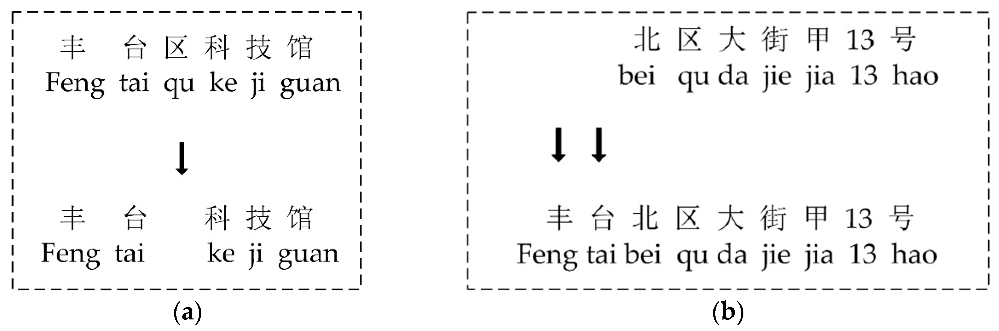
The name is generally considered to be a unique attribute that visually distinguishes geospatial data. Sometimes, however, the same geospatial entity can have both an abbreviation and a full name (e.g., “武汉大学 (Wuhan University)” and “武大 (Wuda)”). The classic method currently used to calculate name similarity is the Levenshtein distance [31]. The Levenshtein distance method consists of calculating the minimum number of edits required to convert one string into another. When calculating the similarity of Chinese sentences, the computational editing distance is traditionally measured in words. In this case, the editing operations are defined as add, delete, and replace. Each operation has a weight of 1. The smaller the editing distance, the more similar the measured values of the two attributes. The calculation of name similarity is performed using Equation (3):
where is denoted as name similarity obtained by using the Levenshtein distance; is the editing distance between ; and are names of two entities, with and being lengths of and , respectively. However, the problem is that in the calculation process, Chinese characters need to be considered as “one character” [32].
Figure 2a shows that the Levenshtein distance between the two Chinese names “丰台区科技馆 (Feng tai qu ke ji guan)” and “丰台科技馆 (Feng tai ke ji guan)” is 1. Figure 2b shows that the Levenshtein distance between the two addresses “北区大街甲13号 (bei qu da jie jia 13 hao)” and “丰台北区大街甲13号 (Feng tai bei qu da jie jia 13 hao)” is 2.
3.5. Address Similarity
The address attribute is similar to the name attribute. Since both are textual in nature, we can measure the similarity using the same method. However, compared with the name attribute, the address attribute has a weaker ability to match POIs. The main reasons are as follows. (1) The uncertainty of address attributes is higher than that of name attributes. For example, addresses with administrative divisions attached and addresses without administrative divisions attached, such as “丰台北区大街甲13号 (Feng tai bei qu da jie jia 13 hao)” and “北区大街甲13号 (bei qu da jie jia 13 hao)”, might represent the same POI. (2) The traditional Levenshtein distance algorithm calculates the Levenshtein distance between strings in a single word. However, in Chinese, a single word usually does not have an actual semantic meaning. For example, “丰(Feng)” and “台(tai)” do not express the meaning of the compound word “丰台(Feng tai)”. (3) The editorial costs between words are not all the same; for example, with “丰台区 (Feng tai qu)” and “丰台 (Feng tai)”, the cost should not be very large.
To solve the problem of the low efficiency of word segmentation caused by sparse training samples, we drew on the idea of Li et al. [29] to construct a word segmentation dictionary of addresses. Using the NLPIR–ICTCLAS Chinese word segmentation system (http://ictclas.nlpir.org), we split the address into a series of word sequences instead of individual characters. For instance, “丰台北区大街甲13号 (Feng tai bei qu da jie jia 13 hao)” was divided into “丰台 (Feng tai)/北区 (bei qu)/大街 (da jie)/甲 (jia)/13号 (hao)” instead of “丰 (Feng)/台 (tai)/北 (bei)/区 (qu)/大 (da)/街 (jie)/甲 (jia)/13 号 (13 hao)”. Then, TF–IDF (term frequency–inverse document frequency) and HowNet were used to extract features and construct feature vectors for segmentation results. Accordingly, we established the word vector and calculated the cosine similarity [33] as the name and address similarity value
Here, denoted the name similarity obtained by using the cosine similarity, and were components of vector and , respectively. Take “丰台北区大街甲13号 (Feng tai bei qu da jie jia 13 hao)” and “北区大街甲13号 (bei qu da jie jia 13 hao)” as examples. and ; the cosine similarity was 0.89, and the address similarity calculated using the Levenshtein distance was 0.78.
3.6. Category Similarity
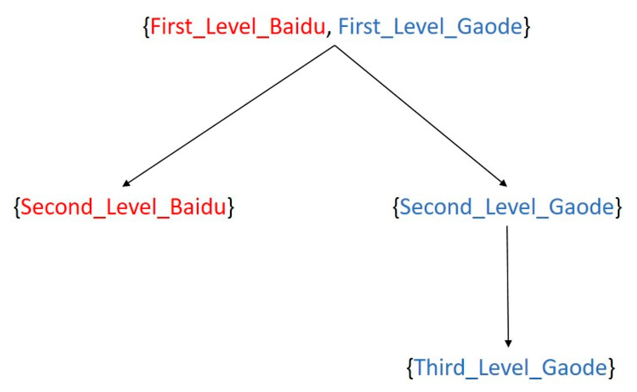
To a certain extent, categories of POI can aid us in finding matches to some degree. Category similarity can reflect the similarity of POI entities [29,34], and POIs of the same category are more likely to be similar than POIs of different categories. For example, a “park” type is more similar to a “botanical garden” type than to a “school” type. Regarding the experimental data in Section 4.1, both the Baidu Map and Gaode Map have established their own category systems to help users find a certain type of POI. The Baidu Map POI category system has 19 first-level categories and 138 second-level categories; in contrast, the Gaode Map POI category system has 23 first-level categories, 264 second-level categories, and 869 third-level categories. The data producer can label new POIs according to the category system.
To address the difficulty of similarity calculation caused by different POI data category systems from different sources, we calculated the category similarity in two steps. First, we integrated the two POI category systems mentioned above. represents the Baidu Map POI category system, while represents the Gaode Map POI category system. represents the POI category system after integration. represent first-level category labels, represent second-level category labels, and represents a third-level category label. For the first-level category , we established a connection between them; thus, , such as {Food, Catering Service}, {Shopping, Shopping Service}, {Medical, Health Care Service} and so on. For a category that did not find corresponding object, we added them as complements to the category fusion system, such as {Event Activities} and {Indoor Facilities}. For the second- and third-level categories, we traced the POI category tree and assigned its parent category. An example is shown in Figure 3.
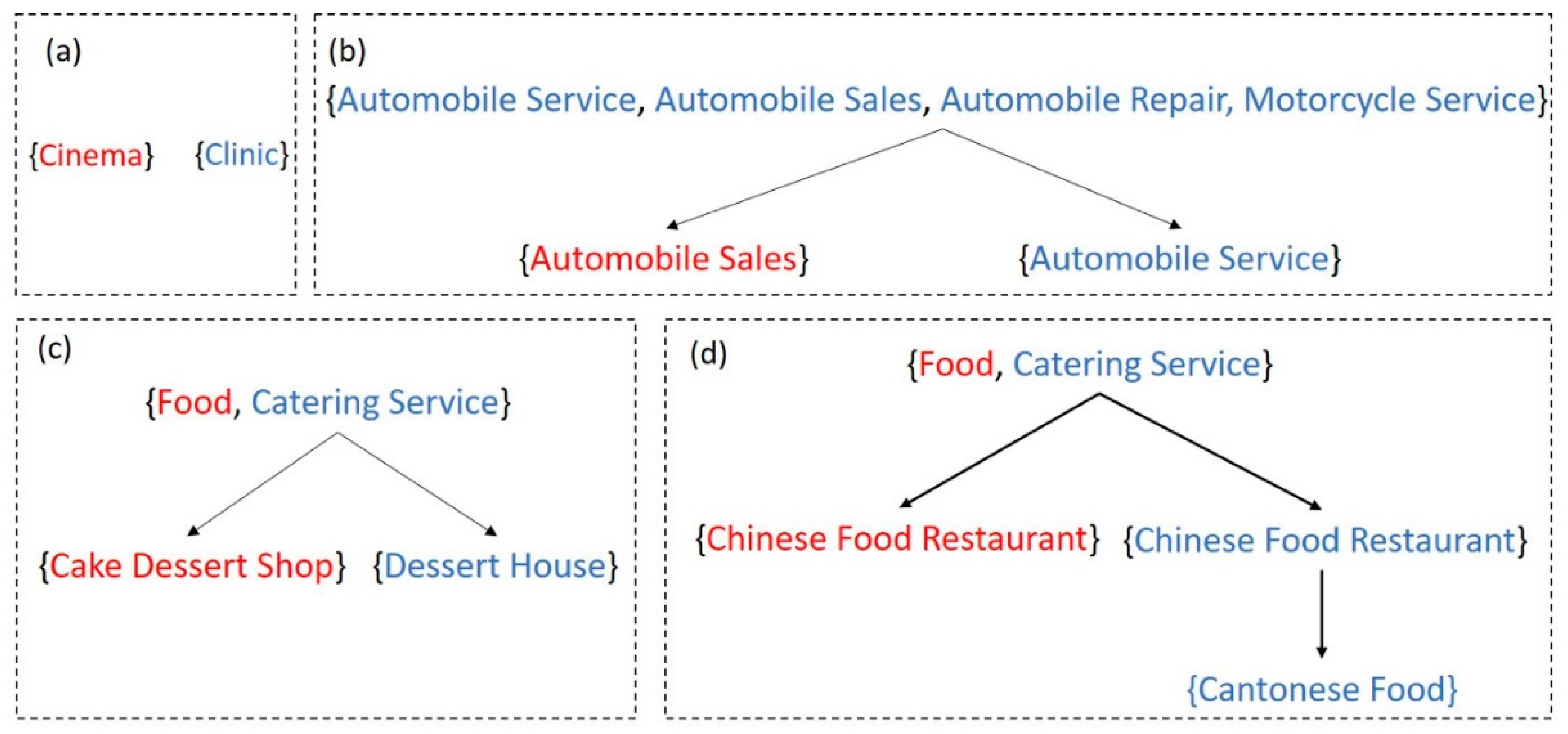
In the second step, the category similarity was obtained by calculating the distance between any two tree nodes (using Equations (5) and (6)).
Here, denotes the distance between the nodes; denotes category similarity; and are any two nodes of the tree; represents the distance between the two nodes; and represent the distance from their shared parent node to the first node and the second node , respectively; and is the maximum distance, which could be derived either from the dataset or the preset for a domain [5]; in this paper, equals 3. We considered the following four situations—(1) {Cinema} was a second-level category in the Baidu Map, {Clinic} was a third-level category in the Gaode Map, and there was no shared parent node between them; the distance between them was , thus, the category similarity between them was 0 (Figure 4a). (2) {Automobile Service} was a first-level category in both the Baidu Map and the Gaode Map. They shared the same parent node and were also their own parent nodes; the distance between them was 0 (Figure 4b). (3) {Automobile Sales} was a second-level category in the Baidu Map, a first-level category in the Gaode Map, and the first-level category was a shared parent node between the categories in the two systems; the distance between them was 1 (Figure 4b). (4) {Cake Dessert Shop} was a second-level category in the Baidu Map, {Dessert house} was a second-level category in the Gaode Map, and {Food, Catering Service} was a shared parent node between them; the distance between them was 2 (Figure 4c). (5) {Chinese Food Restaurant} was a second-level category in the Baidu Map, {Cantonese Food} was a third-level category in the Gaode Map, and {Food, Catering Service} was a shared parent node between them; the distance between them was 3 (Figure 4d).
3.7. The Improved D–S Evidence Theory Method
Research by McKenzie et al. [28] showed that methods that combined multiple attributes were more suitable for inaccurate attribute values than methods that used a single attribute. However, the results of similarity calculations that use different attributes might create conflicts. For example, the Chinese Art Museum and the “Chinese Art Museum Restaurant” were located at “No. 1 Wusi Street”. They might be different POIs when they were measured by their name similarity, but they were matched POI pairs when measured by their address similarity. D–S evidence theory was an uncertain reasoning method that allowed people to model and reason about problems of inaccuracy and uncertainty, and allowed the whole problem and evidence to be decomposed into several sub-problems and sub evidence [35]. After dealing with the sub-problems and sub-evidence, correspondingly, the D–S combination rule was used to obtain the solution of the whole problem [36]. At the same time, the evidence theory had a strong theoretical foundation, the description of uncertainty in decision-making was more in line with the people’s thinking habits, integrating the opinions of multiple decision-makers [37]. To apply multiattribute modeling based on the D–S evidence theory, we introduced a set of hypotheses called the frame of discernment, where the hypotheses represented all possible results that come from the multiattribute modeling process. We use and to represent two independent datasets obtained from different sources. If a pair of geospatial entities represent the same entity, where , then they are called a corresponding pair of geospatial entities. The attribute item set was represented by . The similarity calculation was performed for each single attribute , and the results obtained by the types of attribute matching methods were used as independent evidence to construct a basic probability assignment. Integration was performed by the combination rule of the D–S evidence theory, and the final target matching result was given according to the decision threshold. The D–S evidence theory calculation process was as follows:
(1) Frame of Discernment.
In the D–S evidence theory, is called the frame of discernment, and all alternatives are made by the decision maker in the recognition frame. is a subset of the power set .
where is the number of hypotheses in system, and represents the ith hypothesis that reflects the ith possible recognition result.
(2) Basic Probability Assignment.
Assuming that is a discernment frame of a set, is a subset of , and if mapping, then satisfies the following condition:
This condition is called the basic probability distribution function or the basic reliability distribution function based on , which is also called the mass function. Any , represents the degree of evidence for , excluding support for any true subset of . In addition, if , then is called the focal element of .
(3) Belief Function.
The belief function () represents the degree of trust in the event that is true.
(4) Plausibility Function
The plausibility function () describes the possibility that mass function does not regard proposition as false.
Clearly, in the D–S evidence theory, for each hypothesis in the recognition frame , and denote the upper and lower bounds of probability, respectively, which form the uncertainty interval .
(5) D–S Combination Rule
The key to building a multiattribute model system based on the D–S evidence theory is the D–S combination rule. Assuming that the multiattribute frame is , and two pieces of evidence are obtained from two independent attributes. The D–S combination rule can be defined as follows:
where is the evidence conflict factor and .
(6) Improved D–S Evidence Theory
Due to the uncertainty from multiple attributes of POIs, the application of the D–S evidence theory would result in counterintuitive results when the evidence is highly conflicting. These conflict situations are called fuse paradoxes [38]. The method of fusing conflicting attributes is key to matching multiattribute POIs. In Equation (12), situations in which are called complete conflicts; when , they are called incomplete conflicts. The larger the value of , the greater the conflicts, which would lead to counterintuitive results. Moreover, some conflict cases could be found in the work of Ye et al. [39]. Thus, to realize reliable and accurate matching for multiattribute POIs, an improved method for high-conflict evidence is proposed.
When the frame of discernment , the basic probability distribution of evidence satisfies , represents the number of pieces of evidence, and the average value of the basic probability distribution is . Therefore, the average of the basic probability assignments could be used as a minimum criterion for determining whether the results are credible. If the basic probability of the recognition result is lower than the criterion, then the recognition result is not credible. The more the basic probability distribution of the recognition result exceeds the criterion, the more reliable the recognition result. In summary, according to the discriminant standard, combined with the mathematical model to correct the evidence source, the specific improvement method steps are as follows:
(1) Modify the basic probability assignment value according to Equation (13)
(2) Normalize the basic probability assignments corrected by Equation (13), according to Equation (14):
where is the number of .
(3) Using the combination rule, synthesize the normalized basic probability assignment values.
4. Case Study
4.1. Experimental Dataset
(1) Data Sources
To test the validity of the proposed model, we collected POIs in 2018 (for Beijing, China) from the Baidu Map (https://map.baidu.com/) and the Gaode Map (https://www.amap.com/), which are the popular online map service providers in China. Using coordinate correction and data cleaning, we obtained 1,909,518 POIs from Baidu and 2,679,508 POIs from Gaode, which were labeled and , respectively. The selected POIs were required to have geospatial coordinates, a name, a category tag, and a simple address description.
(2) Dataset Preprocessing
We randomly selected 392 POIs in and then matched 323 POIs in . The pairs of POIs were called training dataset which covered catering services, corporate companies, schools, hospitals, shopping services, government agencies, and many other types of POIs. The selection of was manually performed. The construction of the matching model included three steps. (1) The unified coordinate system: The two data sets to be matched were transformed into a unified coordinate system (WGS-8 4 coordinates). (2) Obtaining a set of candidate matching entities: The search radius was set at a certain distance (500 m in this study). By traversing each spatial entity object in the reference data set. The preliminary candidate set was obtained by judging the matching relationship between the two entities by calculating the distance between each spatial entity object and the entity to be matched. (3) Comparison of name and address similarity: After selecting the candidate matching entity set, a similarity calculation was performed on the name and address of the candidate matching objects in the two data sets, and the similarity indicators were combined to determine the matching entities in the candidate set.
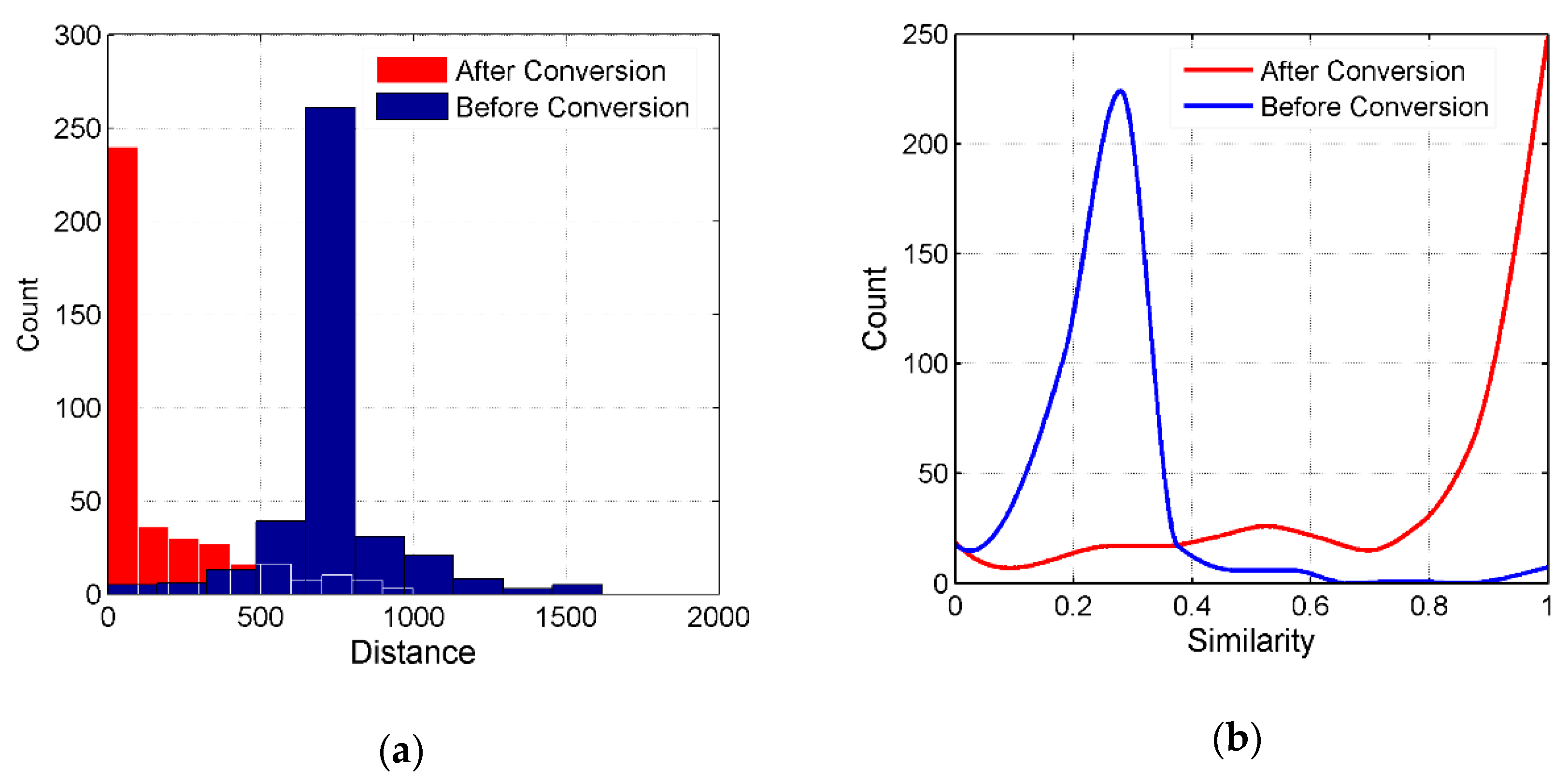
4.2. Spatial Similarity
For the spatial attribute, we obtained the distance between a pair of POIs using Equation (1), for the original coordinates (not converted to a unified coordinate system). The distance of 80% of the POI pairs was 1000 m (as shown by the blue bar in Figure 5a), and several even reached 1600 m. Spatial similarity (as shown by the blue curve in Figure 5b) was obtained from Equation (2). A similarity of 90% of the POI pairs was less than 0.4. Clearly, the original coordinate data could not be used for POI matching due to the inconsistency of the coordinate system. The Baidu Map uses the BD-09 coordinate system, while the Gaode Map uses the GCJ-02 coordinate system. Both coordinate systems were obtained by the WGS-84 encryption. The encryption algorithm causes a nonlinear shift in the data coordinates. To improve the usability of the spatial attribute, we used the application program interfaces (APIs) provided by the two map manufacturers to convert the coordinates (Baidu API: http://lbsyun.baidu.com/index.php?title=webapi/guide/changeposition, Gaode API: https://restapi.amap.com/v3/assistant/coordinate/convert?parameters), and all of them were uniformly transferred to WGS-8 4 coordinates. We recalculated the spatial similarity using Equation (1) and Equation (2) (as shown by the red curve in Figure 5b). The spatial similarity of most matched POIs shifted from 0.2–0.4 to 0.8–1.
4.3. Name Similarity and Address Similarity
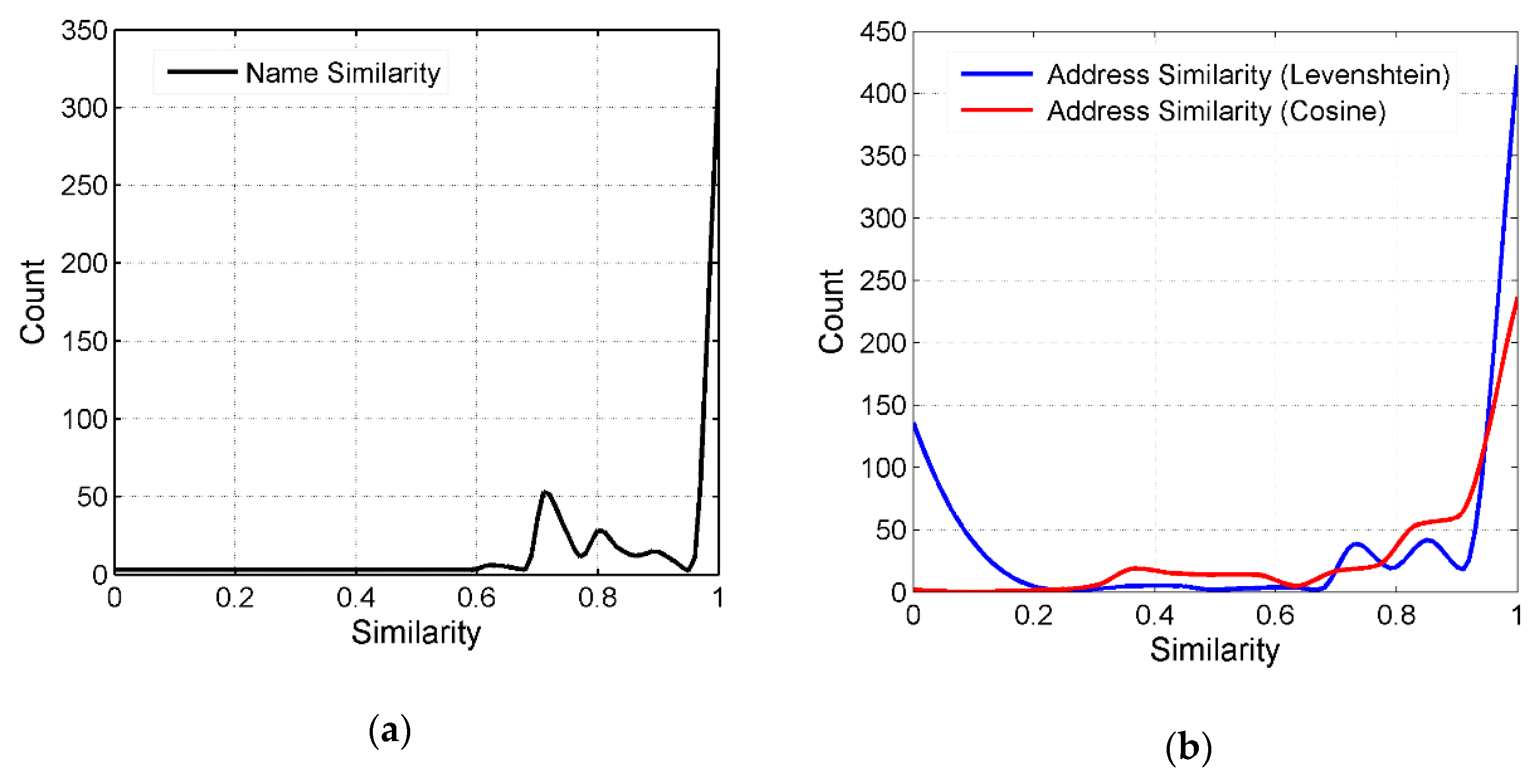
We used the Levenshtein distance (Equation (3)) to calculate name similarity (as shown in Figure 6a). For the address attribute, we used the pre-established address dictionary to segment the addresses of the POI data and then used Equation (4) to calculate address similarity (as shown in Figure 6b).
We found that the name similarity of POIs was between 0.7 and 1 and that the address similarity was between 0.5 and 0.9. From Figure 6, we could make the following observations. (1) The name attribute and address attributes could be used for matching POIs, and in POI matching, the name attribute performed better than the address attribute. The main reason might be that there could be multiple POIs at one address, such as multiple POIs in a commercial building and a number of colleges in a university that used the same address representation. In most cases, however, one POI had only one name. (2) The method of word segmentation using the address dictionary was more suitable for calculating address similarity than the Levenshtein distance. In the subsequent modeling process, only the address similarity values calculated by cosine similarity were used, and the similarity values calculated by the Levenshtein distance were discarded.
4.4. Category Similarity
For the category attribute, in the total 42 first-level categories, except for the {Place Name and Address, Public Facility and Incidents and Events} which were unique to the Gaode Map, the other first categories could find corresponding categories. In the total 402 second-level categories, in addition to 64 of them, the matching category were found to be in all secondary classes. The total 869 third-level categories were traced back to their secondary parent categories. Considering the node depth, we calculated the distance between two nodes representing each pair of POIs. Finally, we used Equation (6) to calculate the similarity characteristics of the category attributes.
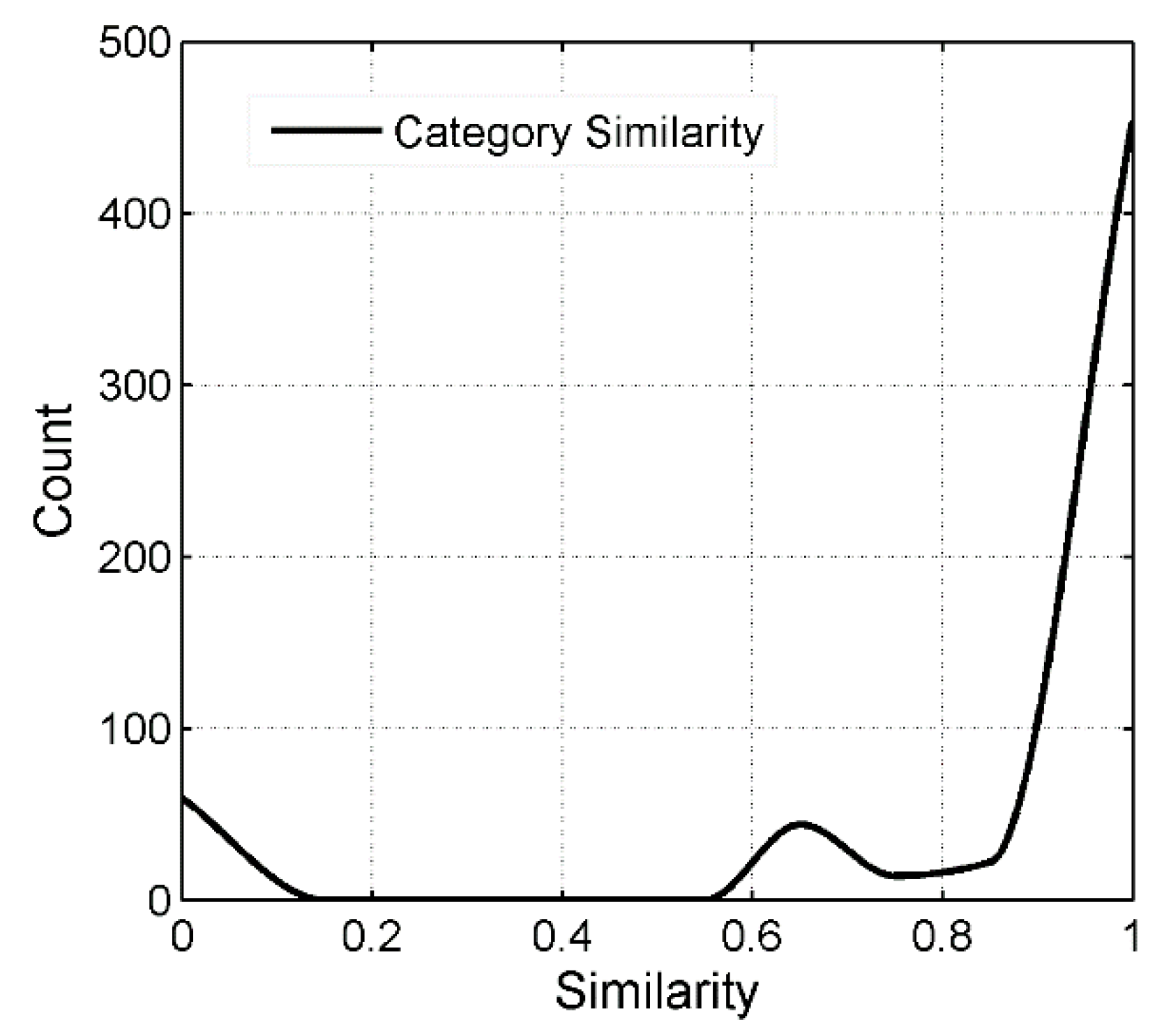
Figure 7 shows the results of counts with varying thresholds of category similarity. From this figure, we could make the following observations—first, a fraction of the similarity values was 0 because some of the categories in dataset Db did not exist in dataset Dg; that is, they did not be correspond completely. At this time, the POI similarity of the two categories was 0. For example, the first-level classification “natural objects” in the Baidu Map category system did not exist in the Gaode Map category system. Second, there was a small peak at 0.61 on the category similarity curve because most of the POIs contained complete categories; that is, the Baidu Map had a 2-layer category structure, while the Gaode Map had a 3-layer category structure. Therefore, the distance between most POI categories was 2. According to Equation (6), the category similarity was 0.61. (3) Category attributes had strong POI matching capabilities. The conclusions drawn were different from those of previous studies and might be related to the data sources used. The Baidu Map and the Gaode Map have a large amount of overlap in the category system.
4.5. The Improved D–S Evidence Theory Model Analysis
4.5.1. Simulation Calculation
To further verify the feasibility of the algorithm, the D–S evidence theory and the improved D–S evidence theory were simulated for evidence combination in different situations, and the integration results were compared and analyzed. Three simulation examples (complete conflict paradox, 0 trust paradox, and 1 trust paradox) were given to illustrate how the improved D–S evidence theory method solved the problem of attribute similarity conflict synthesis. The frame of discernment was , and the evidence contained . The results are shown in Table 1, Table 2 and Table 3.
4.5.2. Multiattribute Model Entity Analysis
In the D–S evidence theory, the pivotal problem is obtaining a basic probability assignment. In this study, we used the similarity of each attribute as the basic probability assignment. To obtain different calculation models and optimal attribute combinations, we constructed two-attribute models, three-attribute models, and a four-attribute model.
After obtaining the basic probability assignment , we used Equation (13) to calculate the similarity of entities after evidence combination, and then, we set a series of thresholds and compared them to entity similarity . If , then the two POIs were identically matched. We used three indicators to evaluate the results of the match—precision, recall, and F1.
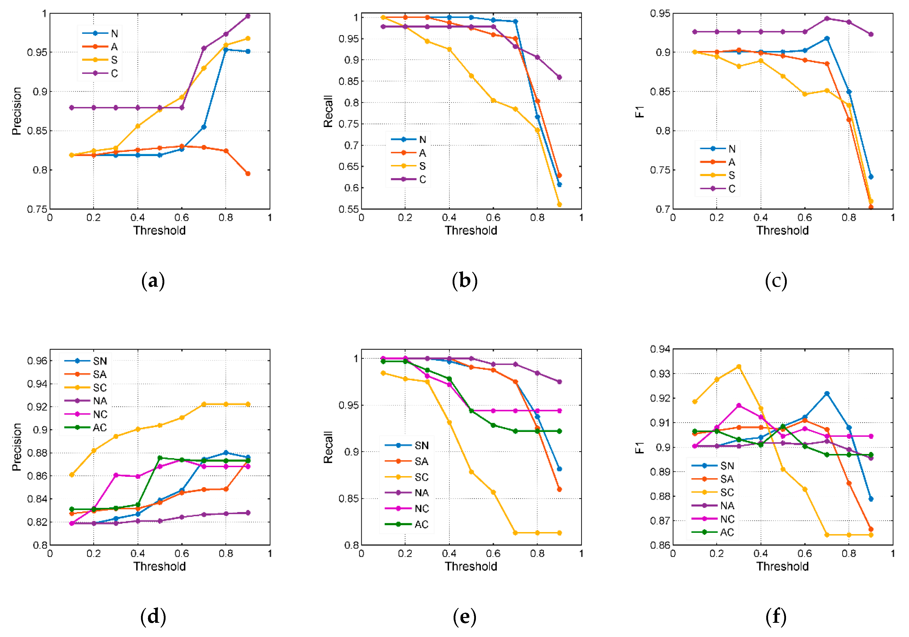
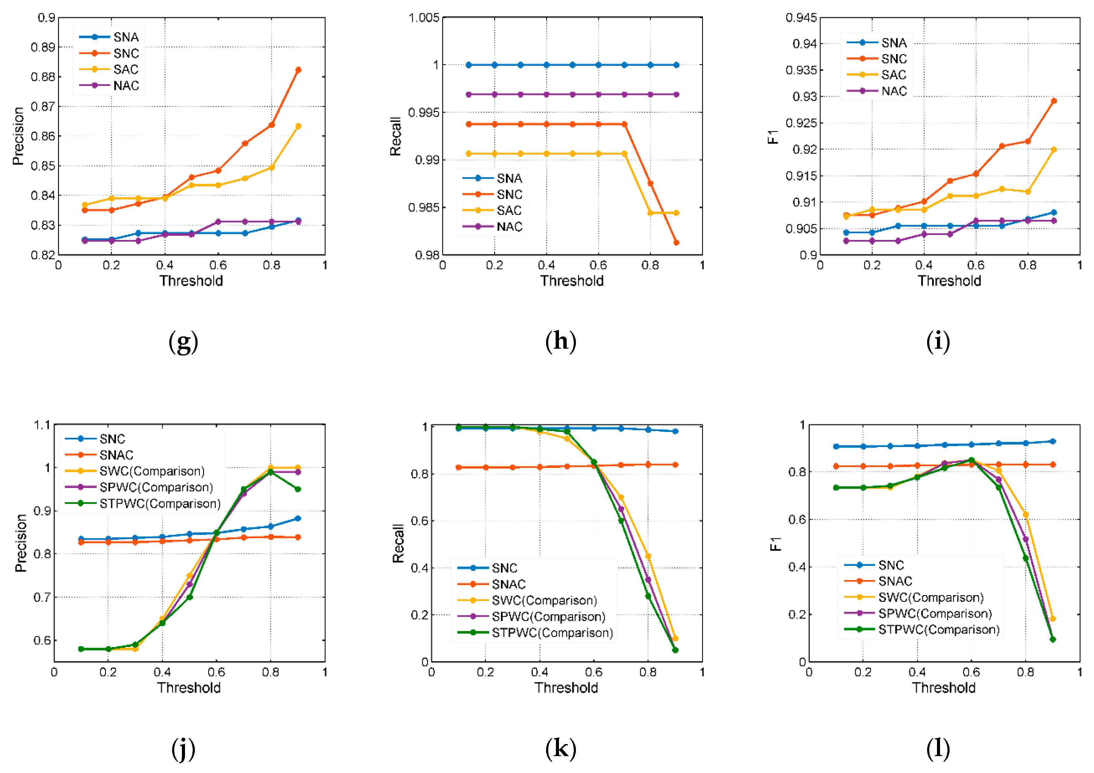
(1) Precision was defined as the ratio between the number of correct matches predicted to the total number of matches predicted, . The results obtained are shown in Figure 8a,d,g,j. The precision of these models improved the most as increased, but when increased to a certain extent, some models, such as the NA (As shown in Table 4, NA is an abbreviation for two attribute models, N represents a name attribute and A represents an address attribute.) and SN models, showed a small decrease as increases. Comparing the four models with single-attribute methods, we found that the C model had the highest precision. Comparing the six models with the two-attribute methods, we found that the SC model had the highest precision. Comparing the four models with the three-attribute methods, we found that the SNC model had the highest precision, which was even higher than that of the four-attribute SNAC model. In addition, when , the precision of the multiattribute models was better than that of the single-attribute models; however, when , the single-attribute models were obviously more precise at finding the corresponding POI. Additionally, Figure 8g–j showed that the SNC model performed better than the SNAC model, indicating that when some poorly performing attributes were introduced into the model, the results worsened.
(2) Recall was defined as the proportion of positive matches that were correctly identified: . Recall represents the ability to find the corresponding POIs in the dataset, and the higher the recall value, the stronger the ability of the model to find the corresponding POIs. Figure 8b,e,h,k showed that the recall performance of the three-attribute models was better than those of the two-attribute models and the single-attribute models. In the three-attribute models, the SNA model achieved the strongest performance in terms of recall (compared with the SNC, SAC, and NAC models).
(3) F1 was defined as a harmonic mean of recall and precision: . A higher F1 indicated that a model could identify more POIs as matched and that the POIs truly correspond. In practice, we not only tried to obtain a higher accuracy but also had a higher recall rate so that we could find as many corresponding entities as possible and could ensure that the objects truly matched. Figure 8c shows that the spatial attribute was the weakest feature for identifying the POIs. Figure 8i shows that among the three-attribute models, the SNC model achieved the strongest performance in F1, indicating that the SNC model not only increased accuracy but also had a high ability to match more POIs. Figure 8l shows that the performance of the SNAC model was lower than that of the SNC model, which indicated that the model might be affected by address attributes.
Overall, from Figure 8 we learn the following. (1) From strong to weak, the single attributes with the best ability to match POIs were the category attribute, the name attribute, the address attribute, and the spatial attribute. (2) The SNC model could simultaneously achieve both the highest precision and the highest F1; that is, the model could find more corresponding POIs, and the POIs were truly corresponding, especially for a threshold greater than 0.8. (3) All multiattribute models performed better in terms of F1 than the single-attribute models. (4) The SWC (comparison), SPWC (comparison), and STPWC (comparison) models, in Figure 8j,k,l were obtained by Li et al. [29]. These models were entropy-weighted multiattribute models. In the early stage, spatial, name, and category attributes were selected through a multi-attribute selection strategy. For each of the above-described attributes, they proposed the calculation of attribute similarity, and then presented a series of entropy-weighted multi-attributes models to combine these attributes together. Comparing the best-performing models with the SNC and SNAC (the best models we obtained) models, we could conclude that the models we obtained (SNC and SNAC), despite their low precision when , had a higher ability (F1) to match more POIs. In addition, the precision, recall, and F1 value of the models remained stable at a higher value and were not affected by a change in the threshold. Clearly, performance was stable.
5. Conclusions and Future Work
Regarding the explosive growth in geospatial data, improving data availability through effective data integration was crucial, but the lack of global identifiers for geospatial data from different sources made data integration challenging.
In this work, we addressed the problem of matching POIs from the Baidu Map and the Gaode Map. The presented work focused on the first step of geospatial data integration, namely, identifying whether two information entities referred to the same place in the physical world. First, we proposed rules for geospatial data attribute selection, analyzed the similarity calculation methods for each attribute (spatial, name, address, and category), and obtained a multiattribute matching model, based on the improved D–S evidence theory. Second, the address attribute achieved poor performance under the traditional Levenshtein distance algorithm, which naturally neglected conceptual disambiguation and linguistic ambiguity. We used the word segmentation method to improve the contribution rate of the names and addresses in the POI matching process. Finally, to address the inaccuracy of geospatial entity matching and the nonlinear similarity feature of nondeterministic attribute items, using a single attribute, we used the improved D–S evidence theory to fuse individual attributes to obtain the final decision result. Our experiments showed that the method based on the improved D–S evidence theory could be effectively applied to the matching of multiattribute geospatial data. This work provided strong evidence that the D–S evidence theory could be used in the field of geospatial entity matching. In practice, we could flexibly set an appropriate threshold value to obtain the corresponding entities at various confidence levels.
In addition, there were a few points that needed attention. First, the precision of POI matching with this method was high, possibly due to the overlap in the category systems between the Baidu Map and the Gaode Map. Second, the model performance of the address attribute was poor, probably because most colleges and hospitals have a large area and there are many internal buildings but all share the same address. For example, both the library and resources and environmental sciences of the information science division of Wuhan University are located at No. 129, Luoyu Road, Hongshan District, Wuhan City, Hubei Province. Third, if the result of the attribute extraction process are different (not only contain name, address, spatial information and category), this method could adjust reasonably well. However, if the data quality deteriorated significantly, the results of this method might also be questionable.
Although the designed method achieved the basic goal, it had several shortcomings. Since this method was designed for data sources with a perfect category system, it was necessary to consider the establishment of a semantic-based category similarity calculation method when data sources might not have had a complete category system. Another issue that was not been addressed in this research was the problem of a word segmentation dictionary of addresses. This study mainly used NLPIR–ICTCLAS Chinese word segmentation system with its own word segmentation dictionary, without expanding the dictionary according to the actual research.
Future work in this area will involve enhancing our model to match additional VGI and non-VGI geospatial datasets and constructing a more complete dictionary of word segmentation. In addition, we should improve the matching accuracy of single attributes by improving the similarity calculation to improve the overall matching accuracy.
Author Contributions
Conceptualization, Yong Wang; Data curation, An Luo; Formal analysis, An Luo; Funding acquisition, Jiping Liu; Methodology, Yue Deng; Project administration, Jiping Liu; Resources, Yong Wang; Software, An Luo; Supervision, Jiping Liu; Validation, An Luo; Visualization, Yue Deng; Writing—original draft, Yue Deng; Writing—review and editing, Yue Deng.
Acknowledgments
This research was supported by the National Key Research & Development Plan of China (project numbers 2017YFB0503601 and 2017YFB0503502).
Conflicts of Interest
The authors declare no conflicts of interest.
References
- Goodchild, M.F. Citizens as sensors: The world of volunteered geography. Geojournal 2007, 69, 211–221. [Google Scholar] [CrossRef]
- Yuan, Q.; Cong, G.; Ma, Z.; Sun, A.; Thalmann, N.M. Time-aware point-of-interest recommendation. In Proceedings of the 36th International ACM SIGIR Conference on Research and Development in Information Retrieval, Dublin, Ireland, 28 July–1 August 2003; pp. 363–372. [Google Scholar]
- Li, S.; Dragicevic, S.; Castro, F.A.; Sester, M.; Winter, S.; Coltekin, A.; Pettit, C.; Jiang, B.; Haworth, J.; Stein, A. Geospatial big data handling theory and methods: A review and research challenges. ISPRS J. Photogramm. Remote Sens. 2016, 115, 119–133. [Google Scholar] [CrossRef]
- Wiemann, S.; Bernard, L. Spatial data fusion in Spatial Data Infrastructures using Linked Data. Int. J. Geogr. Inf. Sci. 2016, 30, 613–636. [Google Scholar] [CrossRef]
- Cueto, K. A feature–based approach to conflation of geospatial sources. Int. J. Geogr. Inf. Sci. 2004, 18, 459–489. [Google Scholar]
- Wang, S.S.; Stefanone, M.A. Showing Off? Human Mobility and the Interplay of Traits, Self-Disclosure, and Facebook Check–Ins. Soc. Sci. Comput. Rev. 2013, 31, 437–457. [Google Scholar] [CrossRef]
- Chen, L.; Roy, A. Event detection from flickr data through wavelet–based spatial analysis. In Proceedings of the 18th ACM Conference on Information and Knowledge Management, Hong Kong, China, 2–6 November 2009; pp. 523–532. [Google Scholar]
- Antoniou, V.; Skopeliti, A. Measures and Indicators of Vgi Quality: An Overview. ISPRS Ann. Photogramm. Remote Sens. Spat. Inf. Sci. 2015, II–3/W5. [Google Scholar] [CrossRef]
- Scheffler, T.; Schirru, R.; Lehmann, P. Matching Points of Interest from Different Social Networking Sites; Springer: Berlin, Germany, 2012; pp. 245–248. [Google Scholar]
- Stankutė, S.; Asche, H. An Integrative Approach to Geospatial Data Fusion; Springer: Berlin, Germany, 2009; pp. 490–504. [Google Scholar]
- Hastings, J.T. Automated conflation of digital gazetteer data. Int. J. Geogr. Inf. Sci. 2008, 22, 1109–1127. [Google Scholar] [CrossRef]
- Beeri, C.; Doytsher, Y.; Kanza, Y.; Safra, E.; Sagiv, Y. Finding corresponding objects when integrating several geo–spatial datasets. In Proceedings of the 13th Annual ACM International Workshop on Geographic Information Systems, Bremen, Germany, 4–5 November 2005; pp. 87–96. [Google Scholar]
- Christen, P. Data Matching: Concepts and Techniques for Record Linkage, Entity Resolution, and Duplicate Detection; Springer Publishing Company, Incorporated: Berlin, Germany, 2012; p. 289. [Google Scholar]
- Wong, E.; Law, R.; Li, G. Reviewing Geotagging Research in Tourism; Springer: Cham, Germany, 2017; pp. 43–58. [Google Scholar]
- Lenzerini, M. Data integration: A theoretical perspective. In Proceedings of the Twenty-First ACM SIGMOD-SIGACT-SIGART Symposium on Principles of Database Systems, Madison, WI, USA, 3–5 June 2002; pp. 233–246. [Google Scholar]
- Wang, J.; Li, G.; Yu, J.X.; Feng, J. Entity Matching: How Similar Is Similar. Proc. VLDB Endow. 2011, 4, 622–633. [Google Scholar] [CrossRef]
- Novack, T.; Peters, R.; Zipf, A. Graph–based matching of points–of–interest from collaborative geo–datasets. ISPRS Int. J. Geo–Inf. 2018, 7, 117. [Google Scholar] [CrossRef]
- Kitchin, R.M. Increasing the integrity of cognitive mapping research: Appraising conceptual schemata of environment behaviour interaction. Prog. Hum. Geogr. 1996, 20, 56–84. [Google Scholar] [CrossRef]
- Safra, E.; Kanza, Y.; Sagiv, Y.; Beeri, C.; Doytsher, Y. Location-based algorithms for finding sets of corresponding objects over several geo-spatial data sets. Int. J. Geogr. Inf. Sci. 2010, 24, 69–106. [Google Scholar] [CrossRef]
- Devogele, T.; Parent, C.; Spaccapietra, S. On spatial database integration. Int. J. Geogr. Inf. Syst. 1998, 12, 335–352. [Google Scholar] [CrossRef]
- Fonseca, F.T.; Egenhofer, M.J.; Agouris, P.; Câmara, G. Using Ontologies for Integrated Geographic Information Systems. Trans. GIS 2010, 6, 231–257. [Google Scholar] [CrossRef]
- Zhu, J.; Wang, J.; Li, B. A formal method for integrating distributed ontologies and reducing the redundant relations. Kybernetes 2009, 38, 1870–1879. [Google Scholar] [CrossRef]
- Li, J.; He, Z.; Zhu, Q. An Entropy–Based Weighted Concept Lattice for Merging Multi–Source Geo–Ontologies. Entropy 2013, 15, 2303–2318. [Google Scholar] [CrossRef]
- Li, X.; Morie, P.; Dan, R. Semantic Integration in Text: From Ambiguous Names to Identifiable Entities. AI Mag. 2005, 26, 45–58. [Google Scholar]
- Kim, J.; Vasardani, M.; Winter, S. Similarity matching for integrating spatial information extracted from place descriptions. Int. J. Geogr. Inf. Syst. 2016, 31, 56–80. [Google Scholar] [CrossRef]
- Liu, S.; Chu, Y.; Hu, H.; Feng, J.; Zhu, X. Top-k Spatio-textual Similarity Search. In Proceedings of the Web-Age Information Management (WAIM 2014), Macau, China, 16–18 June 2014; Li, F., Li, G., Hwang, S., Yao, B., Zhang, Z., Eds.; Springer: Cham, Switzerland, 2014; Volume 8485. [Google Scholar] [CrossRef]
- Safra, E.; Kanza, Y.; Sagiv, Y.; Doytsher, Y. Integrating Data from Maps on the World-Wide Web; Springer: Berlin, Germany, 2006; pp. 180–191. [Google Scholar]
- Mckenzie, G.; Janowicz, K.; Adams, B. A weighted multi–attribute method for matching user–generated Points of Interest. Cartogr. Geogr. Inf. Sci. 2014, 41, 125–137. [Google Scholar] [CrossRef]
- Lin, L.; Xing, X.; Hui, X.; Huang, X. Entropy–Weighted Instance Matching Between Different Sourcing Points of Interest. Entropy 2016, 18, 45. [Google Scholar]
- Vincent, A.; Pierre, F.; Xavier, P.; Nicholas, A. Log–Euclidean metrics for fast and simple calculus on diffusion tensors. Magn. Reson. Med. 2010, 56, 411–421. [Google Scholar]
- Levenshtein, V.I. Binary Codes Capable of Correcting Deletions. Sov. Phys. Dokl. 1966, 6, 707–710. [Google Scholar]
- Zhang, J.; Ouyang, Y.; Li, W.; Hou, Y. A Novel Composite Kernel Approach to Chinese Entity Relation Extraction. In Proceedings of the 22nd International Conference on Computer Processing of Oriental Languages. Language Technology for the Knowledge-based Economy (ICCPOL ’09), Hong Kong, China, 26–27 March 2009; Li, W., Mollá-Aliod, D., Eds.; Springer: Berlin/Heidelberg, Germany, 2009; pp. 236–247. [Google Scholar] [CrossRef]
- Nie, X.; Feng, W.; Wan, L.; Xie, L. Measuring semantic similarity by contextualword connections in Chinese news story segmentation. In Proceedings of the 2013 IEEE International Conference on Acoustics, Speech and Signal Processing, Vancouver, BC, Canada, 26–31 May 2013; pp. 8312–8316. [Google Scholar]
- Sehgal, V.; Getoor, L.; Viechnicki, P.D. Entity resolution in geospatial data integration. In Proceedings of the 14th Annual ACM International Symposium on Advances in Geographic Information Systems (GIS ’06), Arlington, VA, USA, 10–11 November 2006; ACM: New York, NY, USA, 2006; pp. 83–90. [Google Scholar] [CrossRef]
- Zhang, W.; Ji, X.; Yang, Y.; Chen, J.; Gao, Z.; Qiu, X. Data Fusion Method Based on Improved D–S Evidence Theory. In Proceedings of the 2018 IEEE International Conference on Big Data and Smart Computing (BigComp), Shanghai, China, 15–17 Januray 2018; pp. 760–766. [Google Scholar]
- Silva, L.; De Almeida–Filho, A. A multicriteria approach for analysis of conflicts in evidence theory. Inf. Sci. 2016, 346. [Google Scholar] [CrossRef]
- Jiang, W.; Zhuang, M.; Qin, X.; Tang, Y. Conflicting evidence combination based on uncertainty measure and distance of evidence. Springerplus 2016, 5, 1217. [Google Scholar] [CrossRef] [PubMed]
- Zadeh, L.A. Review of A Mathematical Theory of Evidence. AI Mag. 1984, 5, 235–247. [Google Scholar]
- Ye, F.; Chen, J.; Li, Y. Improvement of DS Evidence Theory for Multi–Sensor Conflicting Information. Symmetry 2017, 9, 69. [Google Scholar] [CrossRef]
Figure 1.
A pair of corresponding entities from different sources (Gaode Map and Baidu Map).

Figure 2.
Calculating the Levenshtein distance—(a) name Levenshtein distance and (b) address Levenshtein distance.
Figure 2.
Calculating the Levenshtein distance—(a) name Levenshtein distance and (b) address Levenshtein distance.

Figure 3.
The map of fusion category for different taxonomies (Baidu Map in red and Gaode Map in blue).
Figure 3.
The map of fusion category for different taxonomies (Baidu Map in red and Gaode Map in blue).

Figure 4.
The distance between any two tree nodes. (a) The distance is ; (b) The distance is 0 and 1; (c) The distance is 2; (d) The distance is 3.
Figure 4.
The distance between any two tree nodes. (a) The distance is ; (b) The distance is 0 and 1; (c) The distance is 2; (d) The distance is 3.

Figure 5.
(a) The histogram of distance and (b) the curve of spatial similarity.

Figure 6.
(a) The name similarity attribute and (b) the address similarity attribute.

Figure 7.
The category similarity attribute.

Figure 8.
The precision, recall, and F1 of the one-attribute models and the two-attribute models: (a) The precision of the N, A, S, and C models; (b) the recall of the N, A, S, and C models; (c) the F1 of the N, A, S, and C models; (d) the precision of the SN, SA, SC, NA, NC, and AC models; (e) the recall of the SN, SA, SC, NA, NC, and AC models; (f) the F1 of the SN, SA, SC, NA, NC, and AC models; (g) the precision of the SNA, SNC, SAC, and NAC models; (h) the recall of the SNA, SNC, SAC, and NAC models; (i) the F1 of the SNA, SNC, SAC, and NAC models; (j) the precision of the SNC, SNAC, SWC (comparison), SPWC (comparison), and STPWC (comparison) models; (k) the recall of the SNC, SNAC, SWC (comparison), SPWC (comparison), and STPWC (comparison) models; and (l) the F1 of the SNC, SNAC, SWC (comparison), SPWC (comparison), and STPWC (comparison) models.


Table 1.
Complete conflict paradox.
| Attributes | Similarity | Dissimilarity |
|---|---|---|
| Name | 1 | 0 |
| Address | 0 | 1 1 |
| D–S Evidence Theory | Invalid | Invalid |
| Improved D–S Evidence Theory | 0.5 | 0.5 |
1 Dissimilarity = 1 − similarity.
Table 2.
Zero trust paradox.
| Attributes | Similarity | Dissimilarity |
|---|---|---|
| Name | 0.9 | 0.1 |
| Address | 0.8 | 0.2 1 |
| Spatial | 0 | 1 |
| D–S Evidence Theory | 0 | 1 |
| Improved D–S Evidence Theory | 0.962 | 0.038 |
1 Dissimilarity = 1 − similarity.
Table 3.
One trust paradox.
| Attributes | Similarity | Dissimilarity |
|---|---|---|
| Name | 0.85 | 0.15 |
| Address | 0.2 | 0.8 1 |
| Spatial | 0.1 | 0.9 |
| Category | 1 | 0 |
| D-S Evidence Theory | 1 | 0 |
| Improved D-S Evidence Theory | 0.67 | 0.33 |
1 Dissimilarity = 1 − similarity.
Table 4.
Different methods involving combinations of models.
| Models | ||||||
|---|---|---|---|---|---|---|
| Two-Attribute Models | SN | SA | SC | NA | NC | AC |
| Three-Attribute Models | SNA | SNC | SAC | NAC | ||
| Four-Attribute Models | SNAC 1 | |||||
1 S = Spatial Attribute; N = Name Attribute; A = Address Attribute; C = Category Attribute.
© 2019 by the authors. Licensee MDPI, Basel, Switzerland. This article is an open access article distributed under the terms and conditions of the Creative Commons Attribution (CC BY) license (http://creativecommons.org/licenses/by/4.0/).
Share and Cite
MDPI and ACS Style
Deng, Y.; Luo, A.; Liu, J.; Wang, Y. Point of Interest Matching between Different Geospatial Datasets. ISPRS Int. J. Geo-Inf. 2019, 8, 435. https://0-doi-org.brum.beds.ac.uk/10.3390/ijgi8100435
AMA Style
Deng Y, Luo A, Liu J, Wang Y. Point of Interest Matching between Different Geospatial Datasets. ISPRS International Journal of Geo-Information. 2019; 8(10):435. https://0-doi-org.brum.beds.ac.uk/10.3390/ijgi8100435
Chicago/Turabian StyleDeng, Yue, An Luo, Jiping Liu, and Yong Wang. 2019. "Point of Interest Matching between Different Geospatial Datasets" ISPRS International Journal of Geo-Information 8, no. 10: 435. https://0-doi-org.brum.beds.ac.uk/10.3390/ijgi8100435
Note that from the first issue of 2016, this journal uses article numbers instead of page numbers. See further details here.