CityGML-Based Road Information Model for Route Optimization of Snow-Removal Vehicle


1
Department of Civil & Environmental Engineering, Yonsei University, Seoul 03722, Korea
2
Department of Energy IT, Gachon University, Seongnam 13120, Korea
*
Authors to whom correspondence should be addressed.
†
Current Address: Olivet Institute of Technology, Olivet University, Anza, CA 92539, USA.
ISPRS Int. J. Geo-Inf. 2019, 8(12), 588; https://0-doi-org.brum.beds.ac.uk/10.3390/ijgi8120588
Submission received: 24 November 2019
/
Revised: 12 December 2019
/
Accepted: 16 December 2019
/
Published: 17 December 2019
Abstract
:Infrastructure usability becomes limited during a heavy snowfall event. In order to prevent such limitations, damage calculations and a decision-making process are needed. Snow-removal routing is a type of relevant disaster-prevention service. While three-dimensional (3D) models support these measures, they contain complex information regarding compatibility. This study generates a city-level semantic information model for roads using CityGML, an open standard data schema, and calculates the optimal snow removal route using this model. To this end, constraint conditions are analyzed from the viewpoint of a snow-removal vehicle, and a road network for an optimal route is applied to a 3D road information model. Furthermore, this study proposes a new algorithm that reduces the number of nodes used in the optimal route calculation, and a genetic algorithm is used to find the solution of the formulated objective function. This new algorithm reduces the number of nodes to less than two-thirds that of the original numbers when determining the optimal travel route for snow-removal vehicles in the target area.
1. Introduction
The three-dimensional (3D) city model is one of the methodologies used for coping with disasters. This model provides essential information on the various aspects of disaster management [1,2,3,4,5]. While various studies have verified that the data provided by 3D city models are more accurate than those obtained using two-dimensional (2D) geographic information systems (GISs), inefficiencies still exist in terms of information production and utilization. This is because the development of 3D GISs, which are a relatively new type of system, has been slow owing to the lack of research. In contrast, several studies on 2D GIS technology and related technologies have been performed since their development [6].
Recent studies on city management have focused on creating and applying 3D urban models, which are being extensively utilized [7]. There are various software programs that support 3D city models. However, relying on specific software to create and utilize city models increases the difficulty of accessing the user’s internal data. It also becomes difficult to reuse the models and extend them to real-world applications because the models not based on an open-standard data schema [8]. In other words, ensuring flexible access to the latest information is crucial when using 3D city models [2]. In terms of information flow, data schemas play an essential role in connecting and reusing the information created with 3D information models. Data schemas predetermine the method of expressing specific information items in forms with specific attributes using abstract objects [9]. The utilization of CityGML as a data schema to express the geometry and information of cities has been increasing of late. CityGML, an international standard of the Open Geospatial Consortium (OGC), is an open data model used for storage and exchange of virtual city models [9,10]. It can express the geometry of a city in 3D and semantically express various types of information about the city [7,11].
This study aims to calculate the optimal route of a snow-removal vehicle to support snow-removal operations during heavy snowfall, thus maximizing the usability of the infrastructure. For this purpose, this study first generates a road-information model, a part of the 3D city model, based on a software-independent standard data schema that facilitates access to data within the model. This generated road-information model is then used to calculate the optimal route.
The effect of snow on a city differs from that of rain. Owing to the different physical properties of snow and rain, cities must implement different solutions to address the problems arising from the occurrence of these natural phenomena. For instance, snow, unlike rain, can accumulate. This accumulation repeatedly affects cities, such as by leading to icy roads or creating additional loads on structures and facilities. With regard to the optimal route of a snow-removal vehicle, priorities for emergency situations that require snow removal can be determined using a 3D model after considering the practical limitations. Further, the optimal-route calculation using a 3D model is favorable for deriving data that are difficult to acquire using 2D models [12,13]. However, the network formation used for the optimal-route calculation assumes that vehicles must traverse all nodes in the network, which does not take into account snow-removal areas that need to be removed first [14,15]. Therefore, a new, improved algorithm is needed to calculate the optimal routes efficiently. With the proposed model, a genetic algorithm (GA) can be used to calculate the final optimal route, as has been successfully done regarding problems related to optimal-route calculation [16,17,18,19]. The proposed route-calculation method, based on the standard data schema, is partially applicable to various cases, including road and city components; it is expected that this method can be extended to future studies on other types of urban routes.
2. Related Works
2.1. Optimal-Route Calculation Theory
Snow-removal vehicles using chemical agents experience a limitation in that they need to return to snow control material storage once the vehicles run out of agents. This limitation distinguishes the optimal route problem as the traveling salesman problem (TSP) [20].
The TSP is a case problem; the salesman starts moving from a place called the depot, visits n number of nodes, and then returns to the depot [21]. For example, as illustrated in Figure 1, the traveling salesman starts at the starting node S and returns to the same node after passing all the nodes. As the TSP has a large number of possible solutions, it is classified as a non-deterministic polynomial-time (NP)-hard problem, and it is challenging to find the optimal solution for a realistic size.
One way to solve the problem is to find the characteristics of the nodes, identify which nodes may not be passed through, and eliminate them [22]. This approach considers nodes only for the arc candidate set to reduce the number of computations, which increase exponentially [23]. However, the inability to use the removed node entails the disadvantage of not ensuring the accuracy of the solution obtained using the removed node.
Therefore, an algorithm, which improves the calculation efficiency, is required for the optimal route calculation for this research problem. This algorithm should select nodes to increase the efficiency of the optimal route estimation, and the final solution can be derived from heuristic methods that have been used successfully.
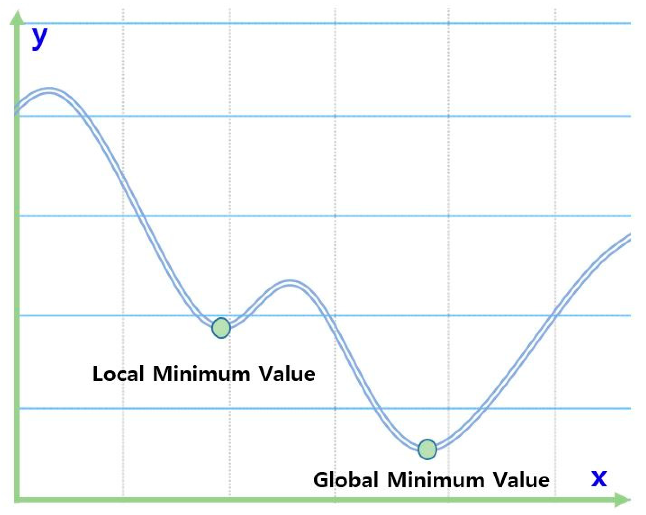
For routing, heuristics uses specific algorithms to determine a better route to destinations. Although the route is not always optimal, heuristics achieve the purpose of determining the route [24]. It is an approximation technique and has proven to be very efficient and powerful in obtaining solutions to real optimization problems with continuous and discontinuous design variables [25]. The technique applies well to specific problems; however, the solution is likely to fall into local optimum values, as shown in Figure 2. Therefore, to find the global optimum value, metaheuristics should be applied, such as GA, harmony search [26], simulated annealing [27], and tabu search [28,29]. Although the global optimum is not always ensured, metaheuristics have high chance to find it within relatively little amount of time for some engineering combinatorial problems such as water network design [30] and multiple dam operation [31]. These metaheuristics are also advantageous as they do not depend on specific computational problems.
This study considers a GA to solve for the optimal route. The superiority of GAs has been demonstrated in comparison with problem-specific heuristic algorithms [32]. Furthermore, the concept and theory of the GA are simple to understand and superior in terms of the derivation of the solution. In particular, a GA is suitable for solving significant computational problems with many variables and constraints, and it is flexible as it can add constraints or change the objective functions [33].
2.2. Three-Dimensional (3D) City Model
The limitations of 2D GIS in addressing real-world problems are becoming apparent, and CityGML is garnering attention as a 3D GIS technology for expressing the geometries of cities. Three-dimensional city models have been used to calculate the heating demand of a city, evaluate photovoltaic potential, and perform noise simulations according to altitude [1,34]. Models for such simulations use various 3D GIS modeling software programs to construct the relevant geometry without semantic information [35]. Virtual 3D city models can be used for visualization only, and the limited usability of the geometric models restricts the extensive utilization of 3D city models. Therefore, a more general modeling approach for 3D urban objects is required in terms of topology and space so as to describe the information requirements of various application fields [7]. As 3D city models including space information consist of spatial factors, such as location, topology, and geometry, and non-spatial factors that represent the characteristics, their structures are far more complex compared to general information. Moreover, such information is constructed in different forms and cannot be properly utilized for various application fields through information linkages. In other words, a consistent and standardized information model is required for the utilization of various application fields through a city information model.
CityGML is a standard data model for storing and exchanging 3D urban information of the OGC [11]. CityGML defines an object-oriented approach for expressing urban objects using technologies such as polymorphism to provide sufficient flexibility [36]. The structure of CityGML is suitable for presenting city models with semantic data. Through this semantic function, the user can perform functions that are not doable without the metadata supported by CityGML [37,38]. CityGML contains the semantic and subject information of a city model in addition to its geometric information. This ensures excellent functions in terms of object integrity, 3D visualization possibility, and scalability of information items or attributes required for comparison with other open standard data schemas [9].
Various studies on CityGML are underway, as is research on the simulation of various aspects of city management using 3D geometric parameters. However, most of these studies focus on creating and managing model information to calculate routes in CityGML models or models based on other standards [39,40,41].
This study uses a CityGML model to calculate the optimal route for snow removal. With the CityGML model, the 3D geometry can be used to utilize the geometrical factors that may arise between the nodes. Moreover, the strengths of CityGML can be utilized to derive meaningful results in future research involving analyses related to other aspects of city management.
3. Methodology
This section presents the CityGML-based 3D routing model and describes the information and the tasks required to determine the optimal route for snow-removal vehicles. The task consists of three main phases for resolving the issues mentioned in Section 2. The first phase consists of analyzing the criteria for roads vulnerable to snow accumulation, to derive the factors for selecting such roads. In the second phase, a road-information model is constructed considering the derived factors. Finally, in the third phase, an improved algorithm is proposed that derives the optimal route considering the priority for snow removal.
3.1. Factors Relevant to Roads Vulnerable to Snow Removal
Snow should be removed quickly to minimize the damage caused by heavy snowfall. Unlike rain, snow can cause secondary damage even after the end of heavy snowfall unless the snow melts because of snow accumulation. It is difficult, however, to remove snow on every road within a certain time period due to limited materials, equipment, and personnel. One possible solution involves stepwise snow removal after deriving priorities by interval and selecting emergency areas.
The concepts of snow accumulation vulnerability and disaster routes can be used to determine the priorities for snow removal. Disaster routes refer to roads designated by the state for temporary management and operation to quickly provide disaster prevention resources to a disaster site [42]. In the United States, disaster routes receive priority for snow removal because disaster routes have priority for the cleaning, repair, and restoration of all other roads in the event of specified disasters, whereas in South Korea, disaster routes are still in the introductory stage [43]. Disaster route selection criteria consist of factors favorable for transportation in snow-affected roads [42] (Table 1).
For roads not included in disaster routes, efficient snow removal is performed to enable civilians to use the infrastructure without restrictions. For this purpose, the snow-removal emergency areas can be derived, considering the vulnerability to heavy snowfall. To determine the vulnerability to heavy snowfall, one of the fallouts of climate change, the concept of vulnerability mentioned in the fifth IPCC report can be used. This refers to various concepts and factors, such as sensitivity to damage in certain climates and insufficient response capability and adaptability [44]. In the field of climate-change research, this vulnerability primarily refers to system attributes that are difficult to address owing to the adverse effects of climate change [45]. The snow-removal priorities for roads can be obtained by applying this concept; as shown in Table 1, information on sunlight, road direction, surroundings of vulnerable spots, slope, traffic volume, and the like can be utilized as evaluation factors [45,46,47,48,49]. As this study used data from South Korea, only snow-accumulation vulnerability was taken into account, considering that the concept of disaster routes was not introduced.
In areas vulnerable to heavy snowfall, the comprehensive factors of exposure, sensitivity, and adaptability simultaneously apply [44]. Climate exposure refers to the degree to which the system is exposed to climate factors owing to changes in temperature and precipitation. Sensitivity indicates how sensitive the system is to the influence of climate, and adaptability is the ability of the system to respond to situations, in terms of socioeconomics [50,51]. However, as this study applies the constraint of heavy snowfall, exposure and adaptability can be excluded from the evaluation factors for selecting roads vulnerable to snow accumulation. Therefore, the roads requiring snow removal can be determined using only the sensitivity factor.
The road facility sensitivity index is based on the geometric conditions of physical structure, technical grade, node-connectivity degree, traffic composition, and the like [45,46,47,48,52]. Among these, to apply the domestic standard, the slope was selected as a factor of the sensitivity, with reference to the road snow-removal task manual in South Korea [52]. According to the manual, road traffic is prohibited in sections with a vertical grade of 6% or higher, and a space for chain installation must be prepared in the front of steep sections with a vertical grade of 4% or higher. However, as passage is considered difficult if the slope of the road is 4% or more, such roads were prioritized for snow removal [42].
Road information such as direction, altitude, road-surface condition, and traffic volume can be considered as additional influencing factors; however, this information is not very systematic at the city and county levels. This study thus attempted to determine the high-priority snow-removal areas by considering only the road length and route width, alternative information that can be obtained relatively easily.
3.2. CityGML-Based 3D Road-Information Model
3.2.1. CityGML Transportation Model
CityGML consists of core modules and several subject modules that contain various types of city objects and their related semantic attributes. This is a semantic information model that combines the attributes according to the geometry and purpose to express the city components in line with the subjects. The CityGML data schema basically defines 12 modules to define the city components. Among these, the ‘transportation module’ is the most relevant subject module that handles the possibility of expressing the distance within different types of models when the application field is the optimal route [53].
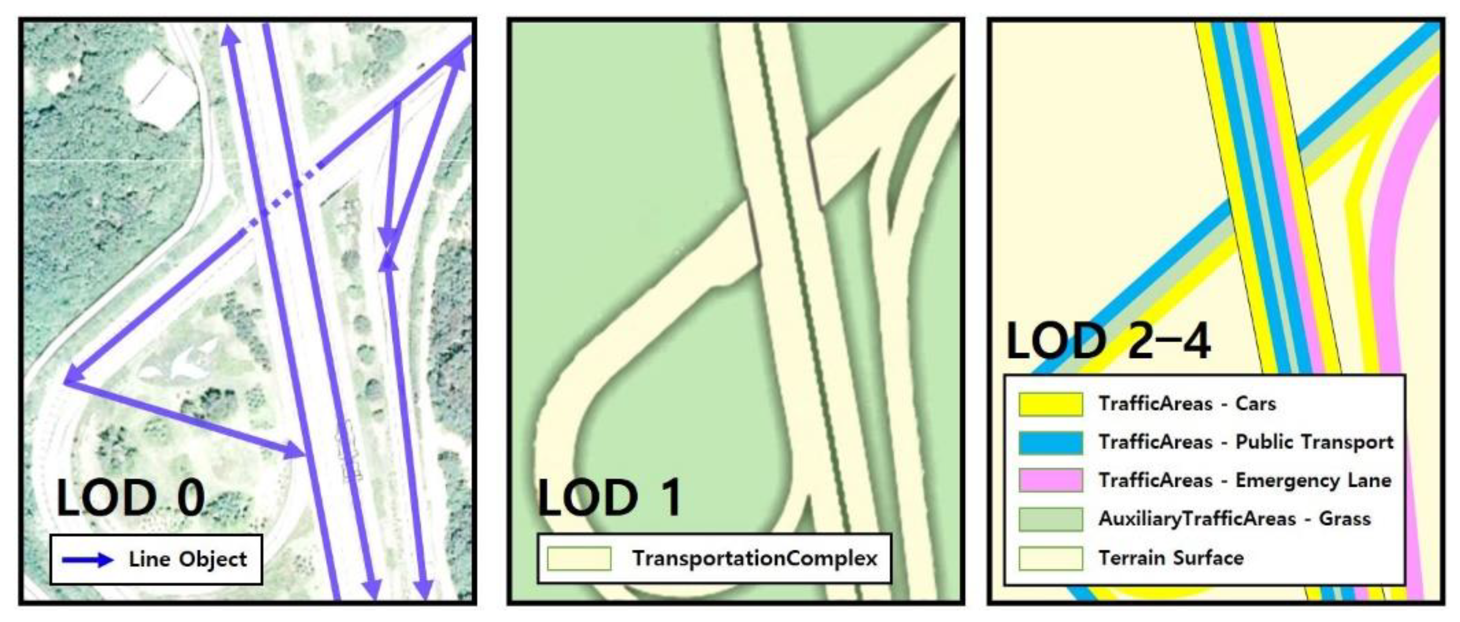
The transportation module consists of road, track, railway, and square. The main class of this model is TransportationComplex, with the subclasses TrafficAreas and AuxiliaryTrafficAreas. The CityGML data schema defines the five levels of detail (LOD) [7,9]; this concept can be introduced to determine the level of detail of the model.
The basic LOD0 can express a linear network, and the more advanced LOD1 can spatially express surfaces. The more detailed LOD2–4 can express driving, lanes, and sidewalks, in which case AuxiliaryTrafficAreas can be expressed; these are objects not directly used for the movement of vehicles or pedestrians. This enables the semantic decomposition of the direct travel route of the vehicle and the parts not directly used.
This study created a data schema for CityGML using the transportation module with LOD1. The factor that determines the LODs is the necessary information for the target application. As mentioned in Section 3.1, the slope, road length, and width are required to calculate the optimal route for snow-removal vehicles. Therefore, the information on LOD2–4 is not needed.
LOD0 enables the use of applications such as path-finding algorithms at an abstract level, and can also schematize and visualize the transportation network. In LOD1, which indicates one higher level of detail, TransportationComplex provides explicit surface geometry by reflecting the actual shapes rather than the centerlines of the road. This study applied the LOD of the road model proposed by the OGC to construct the road schema (Figure 3).
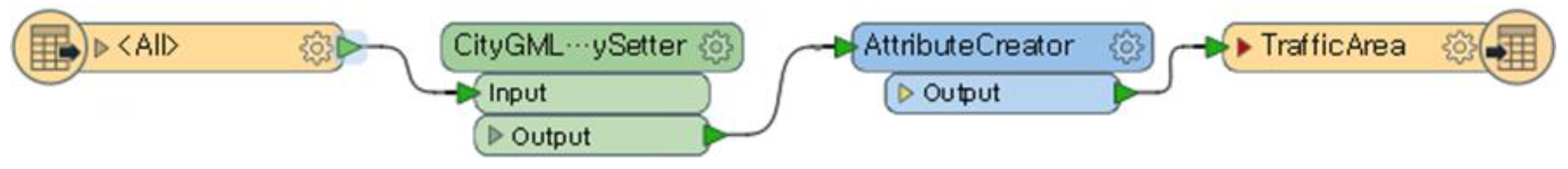
Calculating the optimal route for snow-removal vehicles is advantageous for extracting the slope when reflecting the certain shape of the road width. Accordingly, a LOD1 road network was constructed, and with reference to previous research, the schema components were connected to TrafficArea to construct the CityGML data schema (Figure 4) [54]. This allows the road geometry to have TrafficArea, which is semantic.
3.2.2. Generation of the Terrain-Based Road Model
Creating a model for the 3D geometry and attributes of all roads is challenging. Most administrative departments possess road-design information in a 2D computer-aided design format. As this information is fragmented, creating road models at the city level is difficult. Therefore, in this study, a 3D road model was created under one assumption, namely that the altitude of the terrain is equal to that of the road. The road information model, including terrain information, was developed by applying the altitude values of the terrain information to the road model.
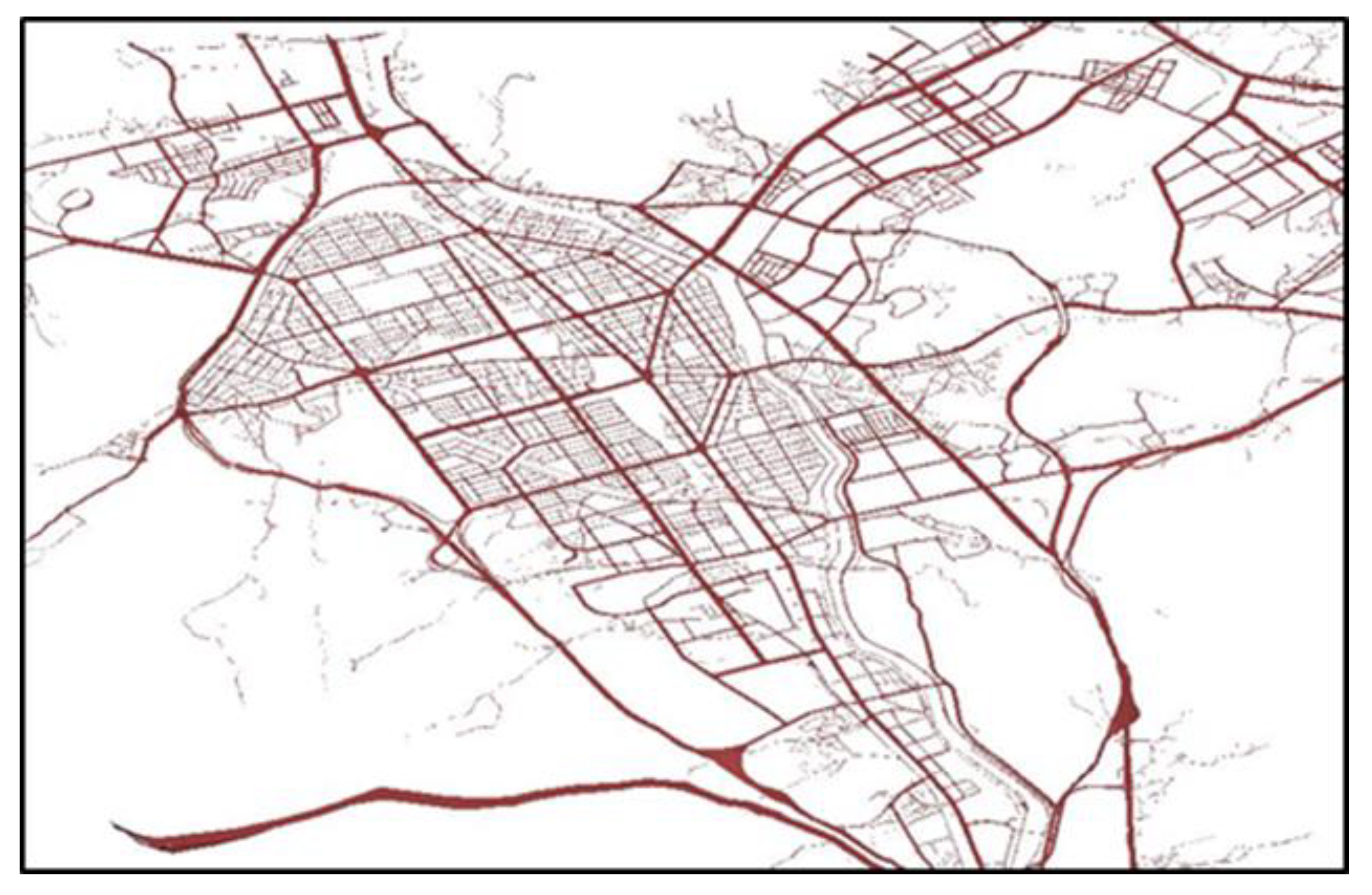
The digital terrain model (DTM) of CityGML is represented in the form of a regular raster, break line, mass points, and a triangular irregular network (TIN) [11]. Among these, the DTM was composed in the form of a TIN, which is often used in 3D engines. With the 3D surface model and 2D road surface created using the digital topographic map data of the target area, the 3D road surface was created using the spatial join function. For this purpose, the TINs containing the z values were created using the altitude, elevation point, and contour line. The points were then extracted from the road surface and combined with the created TIN, giving the z values of the points. From the points, the secondary TIN—which was the final terrain—was created, in which the z values of the elevation point, contour line, and road points were used. Finally, the created geometrical information of the terrain was applied to the road surface, thus generating the final road model. Figure 5 shows the final 3D model.
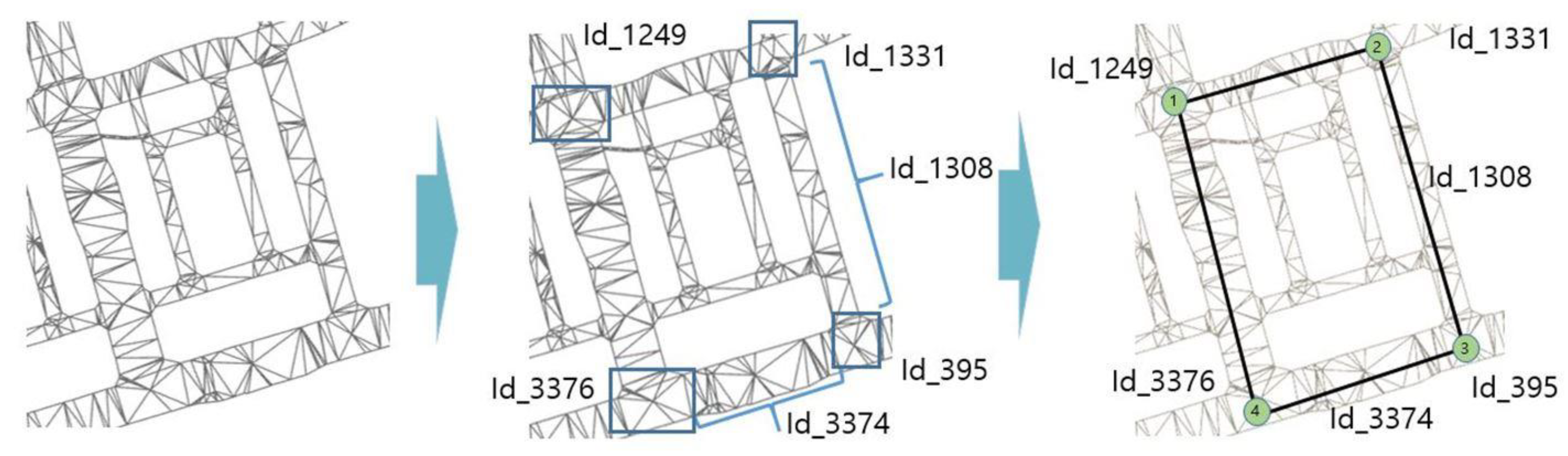
The final CityGML 3D road model can be completed by converting the CityGML data model. This model can be used to generate a network for deriving the optimal route. Therefore, an additional task of linking a network from the CityGML model with GA input data was performed to solve the TSP. The accuracy of the created optimal route network can be increased by assigning IDs to such factors, as shown in Figure 6. The report in OGC [11] that defines CityGML does not provide a methodology for defining IDs. Therefore, in this study, ID numbers were randomly assigned to objects. The IDs are assigned in gml:id form and stored. They are assigned without considering the position and are used as code to identify each object. Further, gml:name can be identified by typing the name of the road hierarchy.
The Bessel coordinate system based on the central datum was used for creating the model. The actual GIS data on a 1/5000 scale were obtained from the Korea National Geographic Information Institute in the form of a digital topographic map. The 2D road surface provided contains traffic island and road length attributes, and it also distinguishes islands and intersections from the roads. Road segments are classified as objects with the length between the intersections. Thus, location information for intersections and traffic islands can be easily used as nodes for the optimal routes, and the road segments that make up the intersection become the distances, as shown in Figure 6.
3.2.3. Slope Analysis Using the CityGML Model
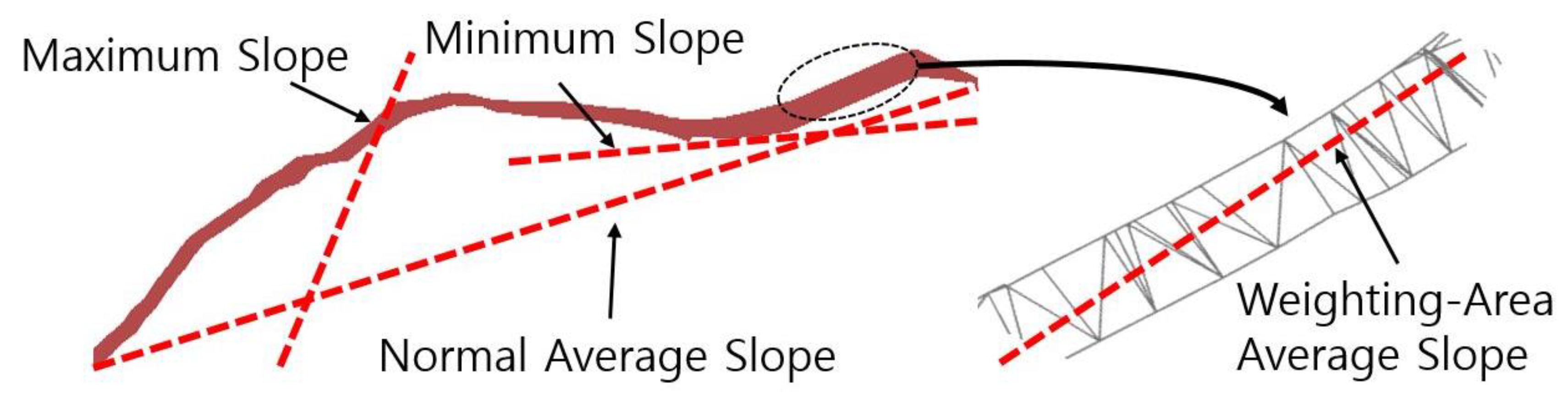
A TIN model for the roads was generated to create the slope needed to calculate the optimal route. In the 3D geometry of the TIN, four types of slopes can be created: maximum, minimum, normal average, and weighting-area average slopes (Figure 7). The maximum and minimum slopes can be appropriately utilized in a graph with smoothly connected and differentiable geometry. However, as road models constructed using a TIN consist of triangular 3D planes and as the slope of each surface is discrete, the maximum and minimum slopes cannot have continuous values. The analysis of the created TIN showed that the slope was too high or too low in certain areas as it was influenced by the local slope. These outlying data are challenging to use as values representing each span of the road in route calculation. Moreover, as the normal average slope is zero if both ends of the road have the same height, the slope at the center of the road cannot be analyzed.
To address this problem, this study analyzed the slope using the weighting-area average slope. This slope is the value obtained by averaging the slopes of all triangular planes in one span; it can yield reasonable results considering that all triangles do not have the same area owing to the nature of TIN.
3.3. Improved Algorithm Considering Snow-Vulnerable Areas
3.3.1. Problem Formularization for Optimal Route Estimation
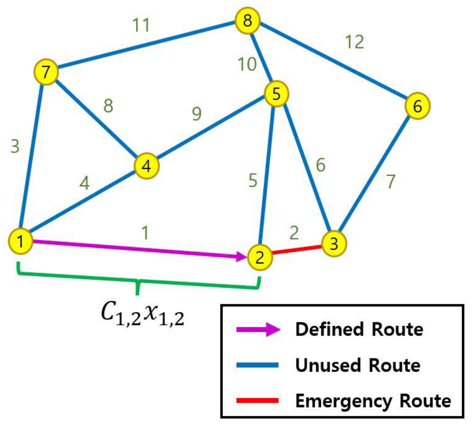
The optimal route for the given problem includes the constraint that the snow-removal vehicle must pass through all emergency roads and return to the snow-removal base. To satisfy this constraint, the sum of all route distances, including those of emergency roads, must be minimized, and the objective function can be set as the total length of all roads. For the total length of all roads, the concepts of departure node i and arrival node j can be utilized, as shown in Figure 8. Movement from one node to another node can be expressed as 1, and the case of not passing through a given node can be expressed as 0. On this basis, the actual route can be obtained as the product of (which indicates whether the route between two given nodes was passed) and (which indicates the distance between the two nodes). This is shown in Equation (1):
Furthermore, as the number of nodes that can be reached from one node must be restricted to one, the following equations must be added:
Moreover, when the constraint condition of the emergency road is presented by the section between nodes 2 and 3, the number of passes from node 2 to node 3 and that from node 3 to node 2 must be restricted to 1 considering that the section must be passed at least once. When the solution of the TSP is calculated using these constraint conditions, a solution containing the fixed distance between nodes 2 and 3 can be obtained. The constraint conditions can be expressed as:
3.3.2. Virtual Route Algorithm
The general TSP solution is inefficient due to unnecessary node not included in the emergency roads. Moreover, since the TSP problem belongs to the class of NP-hard problems, it is difficult to obtain the optimal solution within a limited time, specifically when many nodes exist. Therefore, the number of nodes needs to be reduced to the extent possible (Figure 9).
Nodes that do not include emergency roads can be removed before setting the optimal route formula, but roads included within the removed nodes would also not be utilized in that case. To address this issue, we propose the virtual route algorithm (VRA).
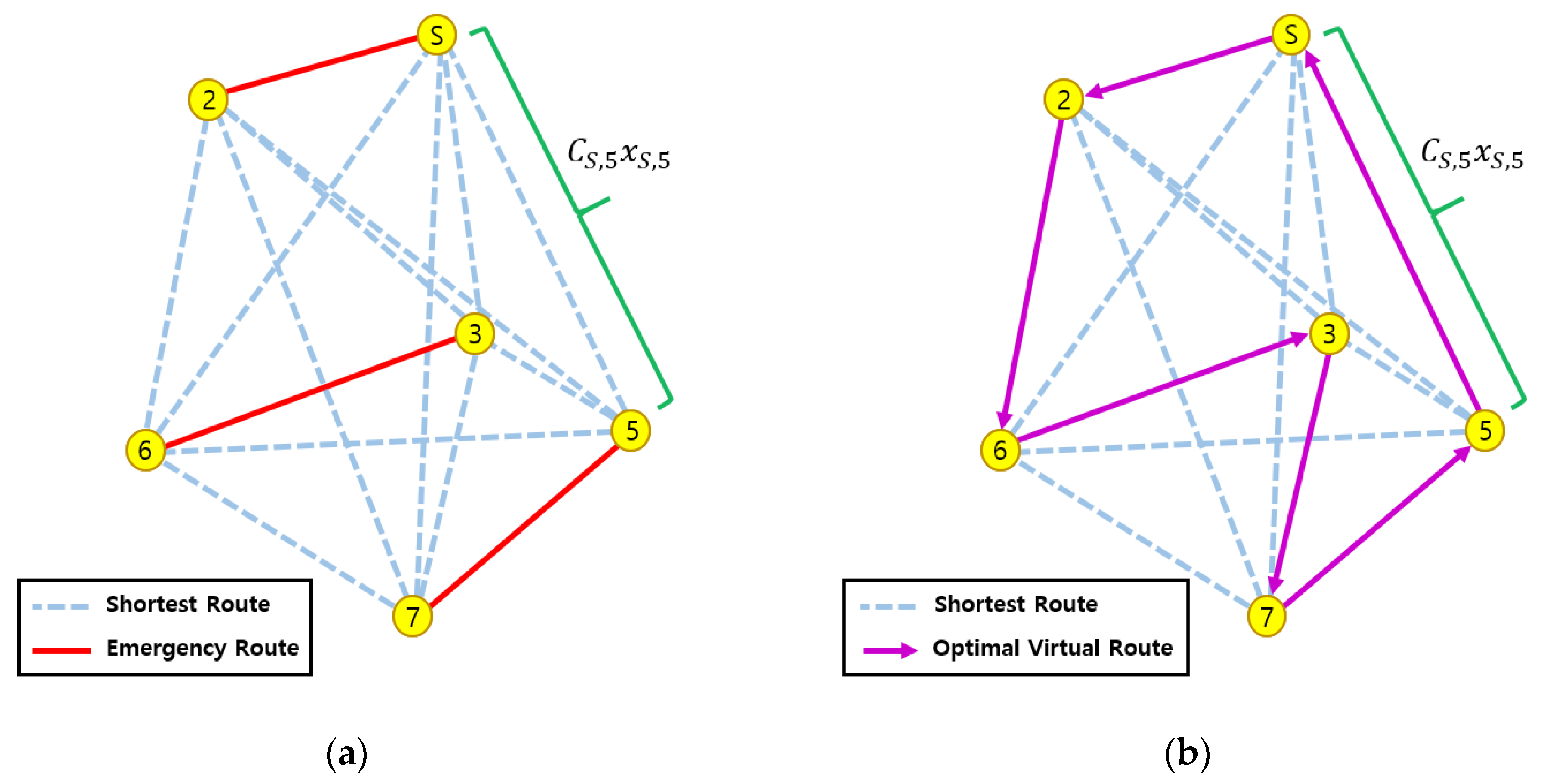
This algorithm first removes nodes 1 and 8 without removing the red lines. However, since the shortest route from node S to node 5 includes node 1, we create the virtual route , which is the sum of the routes and , as shown in Figure 10a. Similarly, node 4, which forms part of the emergency route, can be included as part of the undivided route from node 3 to node 6. This approach allows the development of a new virtual road network that can be used to calculate the optimal virtual route, as shown in Figure 10b.
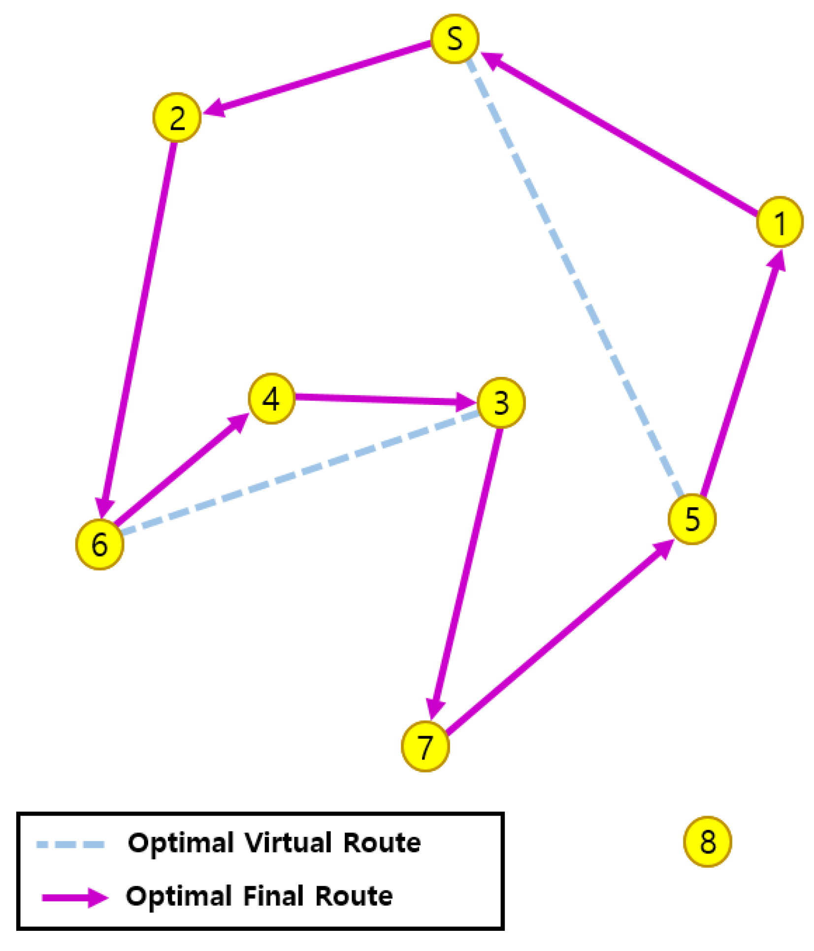
Using these virtual routes, the final optimal route is obtained by separating nodes 1 and 8, as shown in Figure 11. Similarly, node 4, which forms part of the emergency route, can be resolved as an undivided route, , from node 3 to node 6. In conclusion, the VRA adopts only those nodes between both end nodes of the emergency roads as the TSP nodes, but the excluded nodes are included in the optimal route.
The distance required to construct virtual routes is the shortest distance between all the nodes. The Floyd–Warshall Algorithm [55,56] gives the shortest distance for each route to create the new virtual road network. This algorithm is a simple and widely used algorithm that calculates the shortest path between all nodes and checks all the possible paths between all nodes to obtain the shortest distance. The features of this virtually configured network allow the same application of the objective function in Section 3.3.1 and reduce the number of nodes selectively when estimating the optimal route. The VRA is represented as a process in Figure 12.
4. Verification of Optimal Route Calculation for a Real Area
Using the road-information model generated based on CityGML-Transportation, the results of the analyzed slope, and the proposed algorithm for the proposed formularization, this study sought to calculate the optimal route of a snow-removal vehicle during heavy snowfall. The road information that satisfies this purpose was extracted from the generated road-information model, and a road network model for using the proposed objective function and algorithm was constructed. In optimal-route calculation, a GA was used to derive the solution of the proposed objective function.
4.1. Scenario Analysis
Changes in factors such as the number and type of snow-removal vehicles and the setting of snow-removal areas affect the method of calculating the optimal route. In this study, for a real area (including eight districts in Uijeongbu) in South Korea, all the corresponding roads and the roads that must be passed through were selected using the road width and slope. In addition, the scenarios were set only for snow-removal vehicles that use deicers.
The following parameters were applied. Roads with a width of 20 m or higher, corresponding to roads of class 2 or higher as per the Ministry of Land, Infrastructure and Transport (Korea), were selected for this study [57]. Slopes of 4% or higher (i.e., grade E or higher), which are known to pose difficulties for road traffic, were used [42]. Information on the fifth stage of the deicer sprayer regulator was used in line with Table 2 [58]. Moreover, snow removal for areas with a slope of 4% or higher (and not all roads) was targeted. Thus, it was assumed that deicers were not used in areas with a slope of less than 4%, and such areas were excluded.
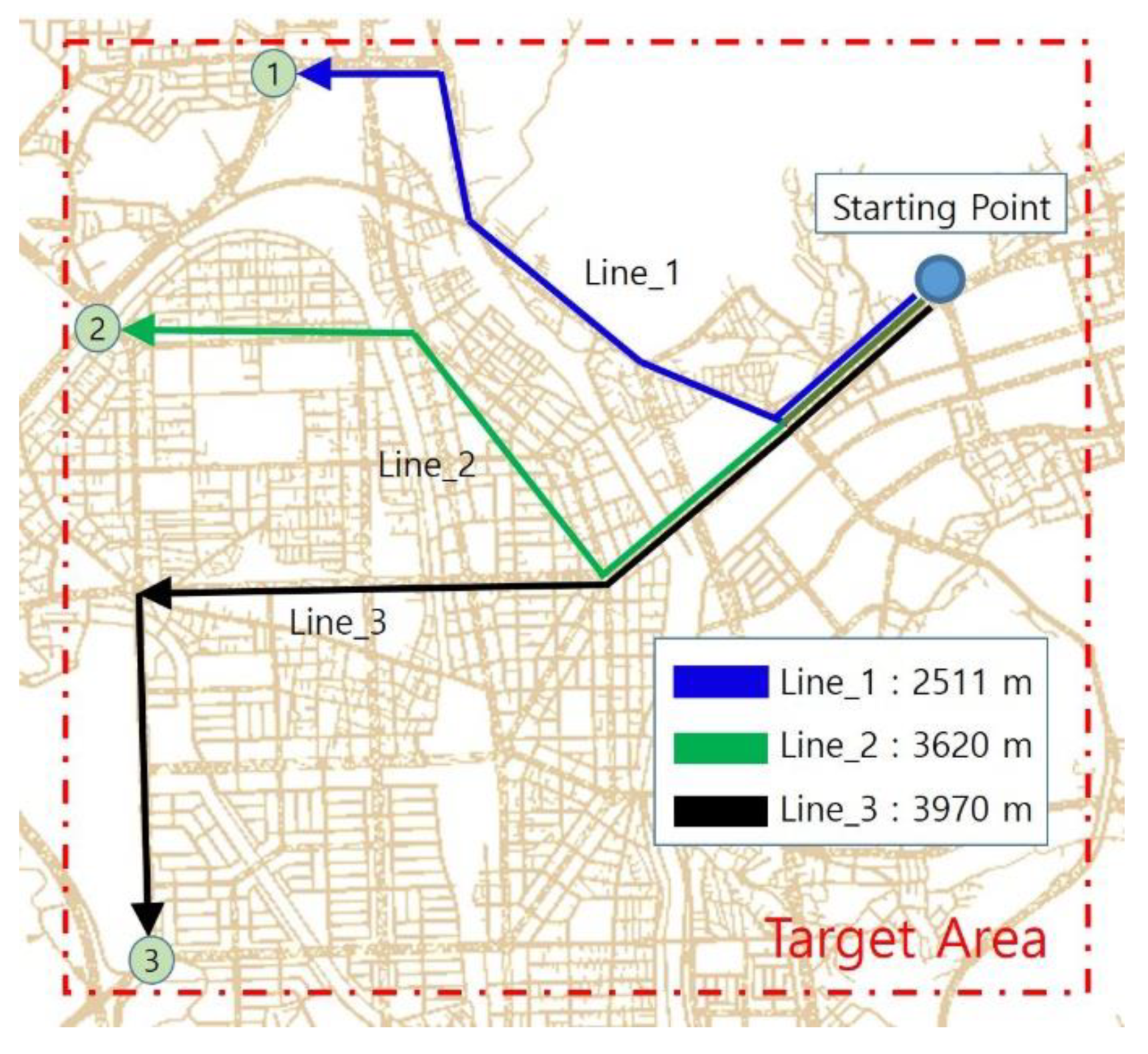
As shown in Table 2, the maximum distance that can be covered by the snow-removal vehicle, from the snow-control-material storage at the first stage of the regulator, is 10 km considering the spray duration and the speed of the vehicle; considering the return of the vehicle, the maximum distance is 5 km. However, as practical conditions may have an influence, a maximum distance of 4 km was used. Figure 13 shows the location of the starting node considering a maximum distance of 4 km from the snow-removal base, derived using the Dijkstra algorithm [59]. This algorithm calculates the shortest distance between two points.
4.2. Road Network Formation
A network is used to simplify the optimization of the actual route. This network is a system of interconnected elements and can visualize roads connecting cities or interconnected streets from an intersection with a series of lines [13]. When a network is completed, optimization can be performed using the proposed and GAs. Table 3 shows the information used in the formation of the road network in this study.
To generate the road network using CityGML, the attribute information was tabulated using FME Workbench. The extracted information includes the slope under the scenario conditions, the total length of all roads, and the road width. This study assumes that the information on the intersections and traffic islands only serves to easily determine the position of the nodes in order to calculate the optimal route. As such, the areas of the intersections and traffic islands were zero.
As shown in Figure 14, the required attributes of the road network can be identified by matching the IDs provided in the creation of the road-information model, using the geometrical information.
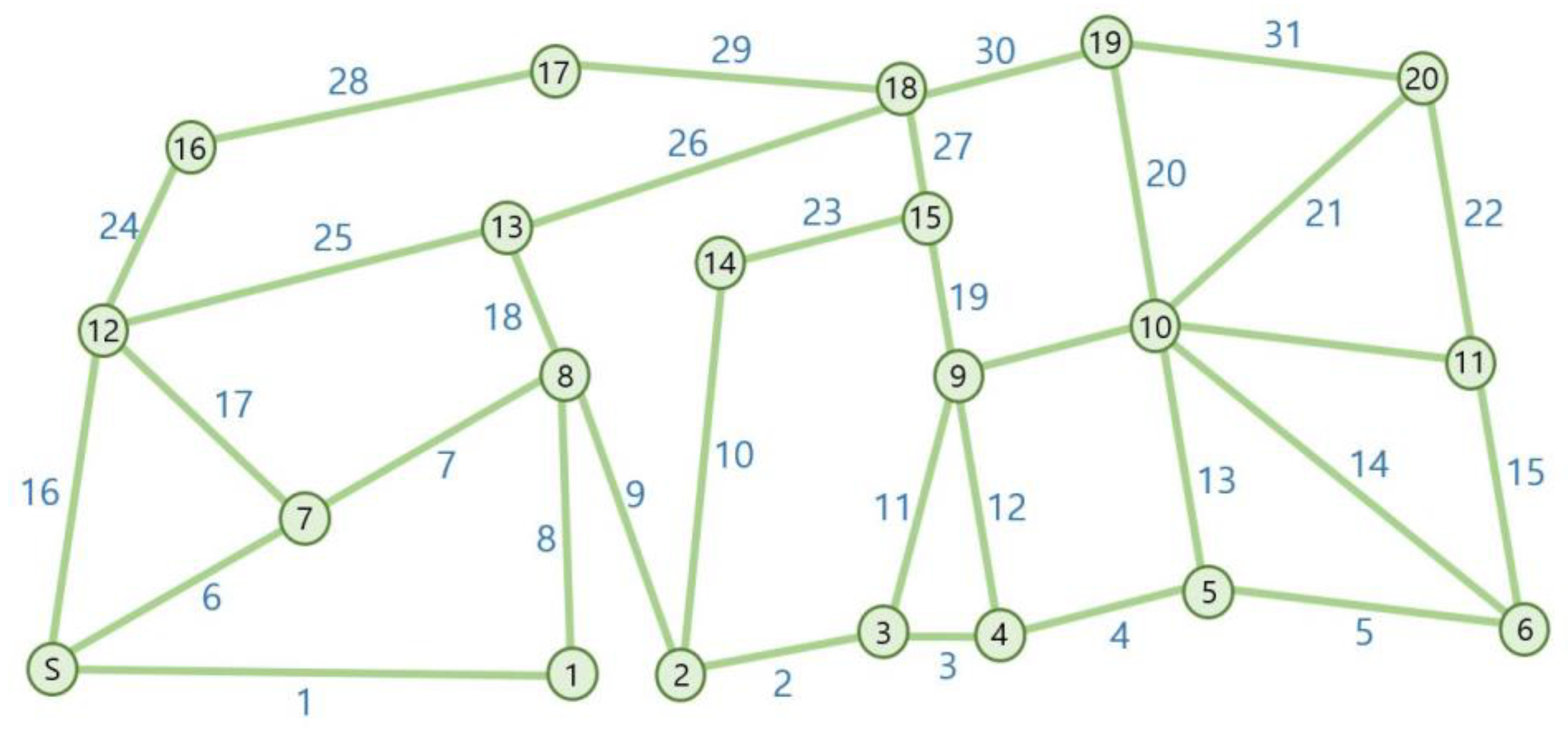
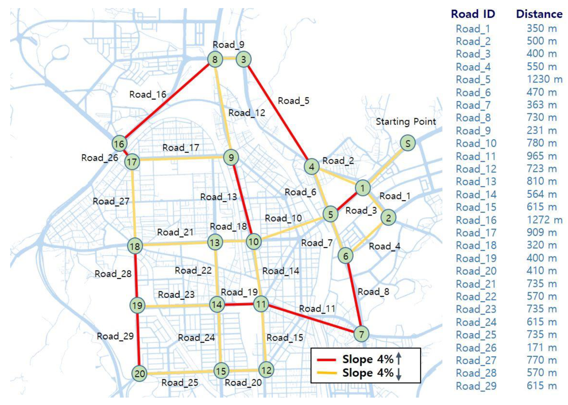
The final network can be formed using the information identified through the IDs. The extracted information was used to form the road network model, as shown in Figure 15. Areas with a slope of 4% (2.29°) or higher were marked with red lines.
4.3. Optimal Route Estimation
Since the starting point S of the network shown in Figure 15 is connected to one road, the overlapping of routes is inevitable. Therefore, this problem is resolved by adding the distance of S to 1 twice in the TSP objective function to eliminate the redundant routes in advance. The objective function and constraint conditions for the TSP starting from 1 are shown in Equations (6)–(9).
The red lines, which are emergency routes considering snow-removal vulnerability in Figure 15, must be passed once. The constraints can be expressed as follows:
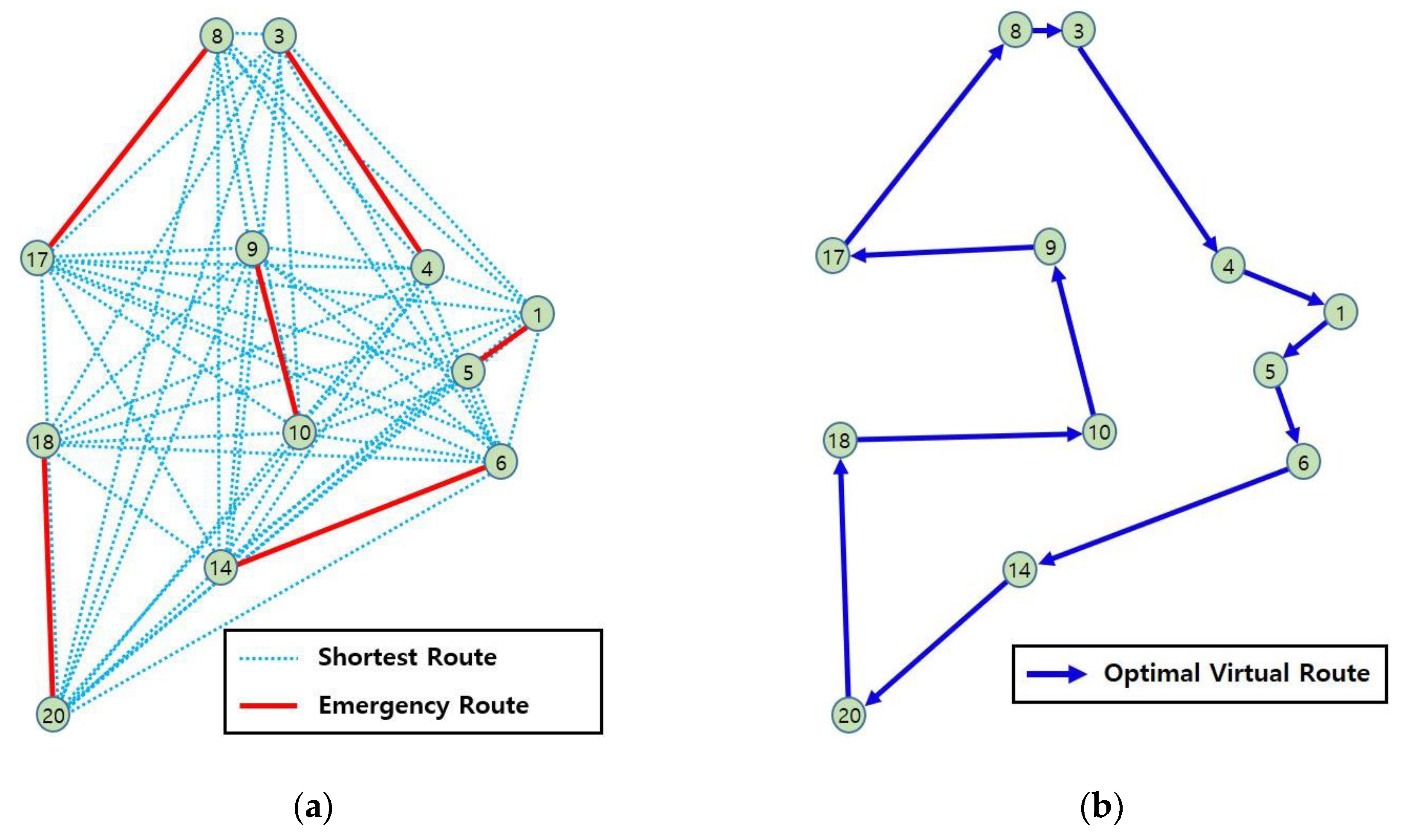
The optimal route, which considers only those routes that must be passed through, can be solved through the VRA. Nodes 2, 12, 13, and 15 are not subject to the above constraint conditions. These nodes and all roads except emergency roads are removed first. In addition, nodes 7, 11, 16, and 19, which are extensions of the essential routes, are removed, and the nodes at both ends of the essential routes can be connected using one virtual road. Thus, 12 (not 20) nodes become the base of the GA . Using these nodes, the shortest distances between the nodes were constructed with the Floyd–Warshall Algorithm (Figure 16a), and the optimal virtual route could be obtained using the GA (Figure 16b).
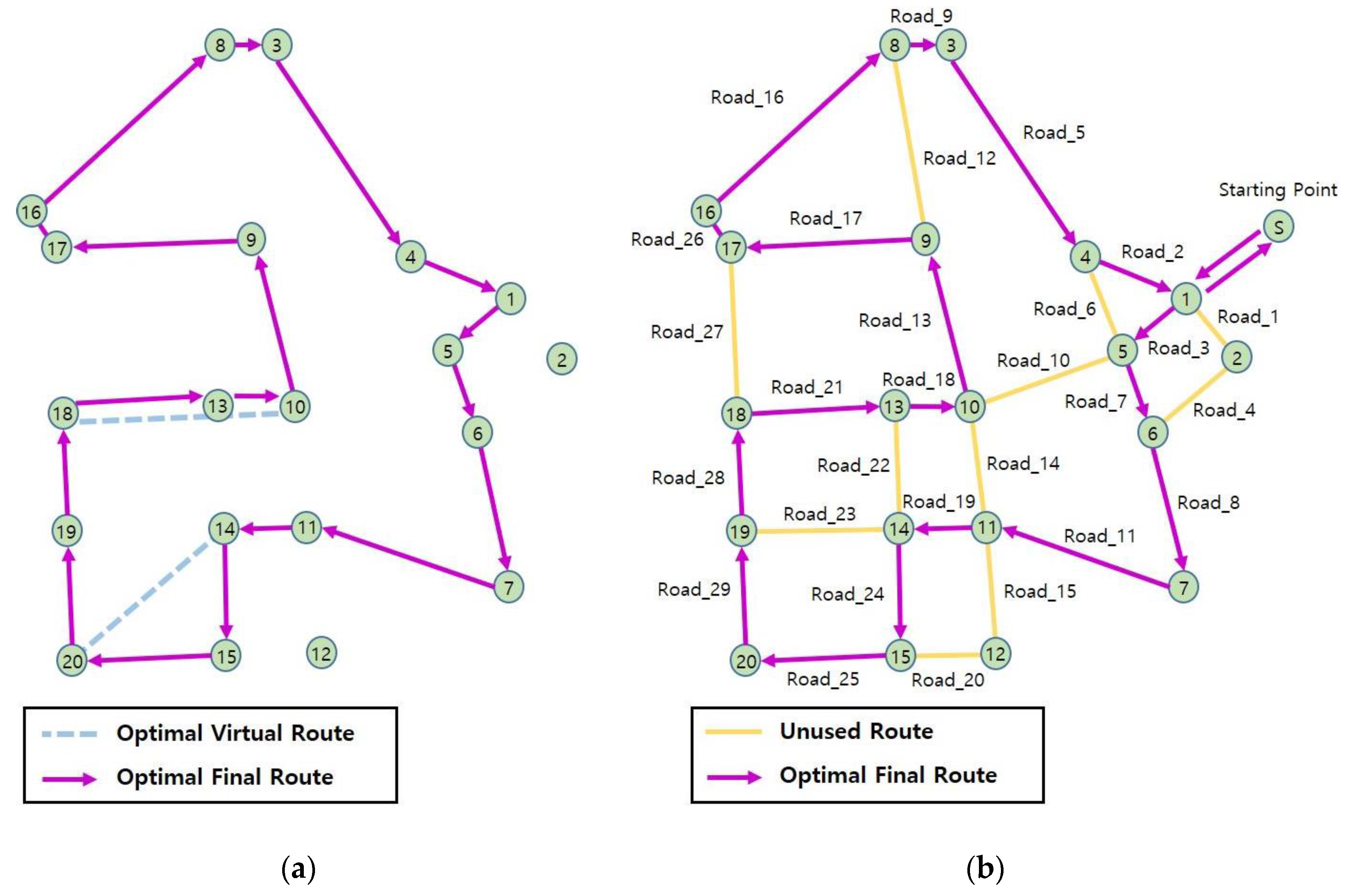
The final optimal virtual route can be obtained by returning the routes of the optimal virtual route to the original road network. As shown in Figure 17a, nodes 13 and 15, which had been removed, were included in the optimal route, and nodes 2 and 12 were automatically excluded from the route. This indicates that nodes that are not necessary for the optimal route can be removed. The optimal final route considering the starting point is calculated using the GA, as shown in Figure 17b. The minimum value of the objective function F(x) is determined to be 12,063 m as the length of the total used extensions, and the length of the total emergency road extensions is 7163 m. Since the snow-removal vehicle in the scenario uses agents only on the emergency roads, this result is within the limited distance range of the snow-removal vehicle in the chosen scenario. Considering that the road is bidirectional, a couple of vehicles can move in the opposite direction of the resulting route to remove snow bidirectionally. Additionally, the scenario in this study involved snow removal using a single vehicle. Therefore, this model has a limitation not to pass multiple lanes in one direction.
Another limitation is that the for the factors affecting the scenario, only factors derived from the fundamental priority were considered; more information may be added to configure more accurate scenarios. These scenarios require a variety of data across cities, and CityGML is useful to implement the scenarios. As mentioned in Section 2.1, a characteristic of CityGML is that it is excellent for data access and can express many city elements simultaneously. Therefore, this study is advantageous for further research on expressing different scenarios.
5. Conclusions
The size of cities and the size and range of damage from disasters caused by climate change continue to increase. Therefore, it is necessary to collect, construct, and utilize information at the city level to secure the usability of infrastructure against disasters. However, information management at the city level is independently performed in each area and the integrated utilization of information is difficult due to reduced interoperability. To address these issues, this paper proposed a method of calculating the optimal snow-removal route by creating and utilizing a model based on a standard data schema.
The necessary factors that need to be taken into account for snow-removal were derived through analysis of road-related standards and data. These factors can be derived from the information or geometrical elements included in roads, which are meaningful data considered in route calculation.
A method of creating a CityGML-based road model was proposed, to create the model for calculating the optimal snow-removal route. A module proposed in CityGML was used to generate semantic information and a model with a low level of detail (LOD) was created to facilitate the creation and management of roads at the city level. To calculate the snow-removal route, the essential information to be considered for the creation of the road model can be collected, analyzed, and reflected in the CityGML road model. Moreover, the model can be easily created using the existing data, and the information can be identified through node information like IDs. This standard model is advantageous in terms of interoperability, which is the basis for its applicability to various fields.
This study also proposed a new algorithm for calculating the snow-removal route. The method of calculating the route with a priority for snow removal can be touted as a traveling salesman problem (TSP). Route calculation using existing methods requires highly complex computation. This study utilized a genetic algorithm and the newly proposed virtual route algorithm to calculate the route. This method is advantageous in terms of computation because only the nodes at both ends of the essential sections are set as the nodes of the TSP. Moreover, as the excluded nodes are also considered, it is advantageous in terms of calculating the optimal route. A model was generated for a real urban area and the optimal route was calculated by factoring in distance and slope, both of which are considered for snow removal. Based on the results, the number of nodes necessary for computation was reduced to less than two-thirds that of the existing method.
The proposed method is superior to the existing method in terms of the reduction of resources required for calculation along with sustained accuracy. The improved algorithm proposed in this study can be comprehensively utilized in various situations for route calculation. In addition, owing to the use of CityGML, which is a standard model for expressing cities, the algorithm applies to various fields such as the analysis of other city elements and events.
Author Contributions
Sang Ho Park designed, conceived, and programmed the new algorithm, as well as analyzed the results. Young-Hoon Jang contributed to generating the CityGML information models and verified the data quality. Zong Woo Geem supervised the research on optimization, and Sang-Ho Lee supervised the development of the CityGML model and extraction of route analysis models.
Funding
This research was supported by the Energy Cloud R&D Program through the National Research Foundation of Korea (NRF) funded by the Ministry of Science, ICT (2019M3F2A1073164). This work was also supported by the Gachon University research fund of 2019 (GCU-2019-0360).
Acknowledgments
The first author (Sang Ho Park) would like to thank Pastor Esther (Jiyoung Kim) at Olivet university for supporting this research.
Conflicts of Interest
The authors declare no conflict of interest.
References
- Biljecki, F.; Stoter, J.; Ledoux, H.; Zlatanova, S.; Çöltekin, A. Applications of 3D city models: State of the art review. ISPRS Int. J. Geo Inf. 2015, 4, 2842–2889. [Google Scholar] [CrossRef] [Green Version]
- Kolbe, T.H.; Gröger, G.; Plümer, L. CityGML: Interoperable access to 3D city models. In Geo-Information for Disaster Management; Springer: Berlin, Germany, 2005; pp. 883–899. [Google Scholar]
- Massaâbi, M.; Layouni, O.; Oueslati, W.B.M.; Alahmari, F. An Immersive System for 3D Floods Visualization and Analysis. In Proceedings of the International Conference on Immersive Learning, Missoula, MT, USA, 24–29 June 2018; pp. 69–79. [Google Scholar]
- Redweik, P.; Teves-Costa, P.; Vilas-Boas, I.; Santos, T. 3D city models as a visual support tool for the analysis of buildings seismic vulnerability: The case of Lisbon. Int. J. Disaster Risk Sci. 2017, 8, 308–325. [Google Scholar] [CrossRef] [Green Version]
- Zhou, Q.; Sun, B.T.; Yan, P.L.; Zhao, P. Study on simulation technology of earthquake disaster scene. In Proceedings of the Advanced Materials Research, Chongqing, China, 21–23 January 2011; pp. 5111–5114. [Google Scholar]
- Irizarry, J.; Karan, E.P. Optimizing location of tower cranes on construction sites through GIS and BIM integration. J. Inf. Technol. Constr. (ITcon) 2012, 17, 351–366. [Google Scholar]
- Gröger, G.; Plümer, L. CityGML–Interoperable semantic 3D city models. ISPRS J. Photogramm. Remote Sens. 2012, 71, 12–33. [Google Scholar] [CrossRef]
- Kar, B.; Hodgson, M.E. A GIS-based model to determine site suitability of emergency evacuation shelters. Trans. GIS 2008, 12, 227–248. [Google Scholar] [CrossRef]
- Lee, S.-H.; Park, J.; Park, S.I. City Information Model-Based Damage Estimation in Inundation Condition. In Proceedings of the International Conference on Computing in Civil and Building Engineering (ICCCBE 2016), Osaka, Japan, 5–8 July 2016; pp. 1038–1043. [Google Scholar]
- Labetski, A.; van Gerwen, S.; Tamminga, G.; Ledoux, H.; Stoter, J. A proposal for an improved transportation model in CityGML. Int. Arch. Photogramm. Remote Sens. Spat. Inf. Sci. 2018, XLII-4/W10, 89–96. [Google Scholar] [CrossRef] [Green Version]
- Open Geospatial Consortium. OGC City Geography Markup Language (CityGML) Encoding Standard 2.0.0; Open Geospatial Consortium: Wayland, MA, USA, 2012. [Google Scholar]
- Schröder, M.; Cabral, P. Eco-friendly 3D-Routing: A GIS based 3D-Routing-Model to estimate and reduce CO2-emissions of distribution transports. Comput. Environ. Urban Syst. 2019, 73, 40–55. [Google Scholar] [CrossRef] [Green Version]
- Tavares, G.; Zsigraiova, Z.; Semiao, V.; Carvalho, M.D.G. Optimisation of MSW collection routes for minimum fuel consumption using 3D GIS modelling. Waste Manag. 2009, 29, 1176–1185. [Google Scholar] [CrossRef]
- Perrier, N.; Langevin, A.; Amaya, C.-A. Vehicle routing for urban snow plowing operations. Transport. Sci. 2008, 42, 44–56. [Google Scholar] [CrossRef] [Green Version]
- Xie, B.; Li, Y.; Jin, L. Vehicle routing optimization for deicing salt spreading in winter highway maintenance. Procd. Soc. Behv. 2013, 96, 945–953. [Google Scholar] [CrossRef] [Green Version]
- Ahmadi, E.; Süer, G.A.; Al-Ogaili, F. Solving Stochastic Shortest Distance Path Problem by Using Genetic Algorithms. Procedia. Comput. Sci. 2018, 140, 79–86. [Google Scholar] [CrossRef]
- Hassanzadeh, R.; Mahdavi, I.; Mahdavi-Amiri, N.; Tajdin, A. A genetic algorithm for solving fuzzy shortest path problems with mixed fuzzy arc lengths. Math. Comput. Model. 2013, 57, 84–99. [Google Scholar] [CrossRef]
- Mohamed, C.; Bassem, J.; Taicir, L. A genetic algorithms to solve the bicriteria shortest path problem. Electron. Notes Discret. Math. 2010, 36, 851–858. [Google Scholar] [CrossRef]
- Zhu, X.; Luo, W.; Zhu, T. An improved genetic algorithm for dynamic shortest path problems. In Proceedings of the 2014 IEEE Congress on Evolutionary Computation (CEC), Beijing, China, 6–11 July 2014; pp. 2093–2100. [Google Scholar]
- Lawler, E.L.; Lenstra, J.K.; Rinnooy Kan, A.H.; Shmoys, D.B. The Traveling Salesman Problem; a Guided Tour of Combinatorial Optimization; Wiley: Chichester, UK, 1985. [Google Scholar]
- Hacizade, U.; Kaya, I. GA based traveling salesman problem solution and its application to transport routes optimization. IFAC PapersonLine 2018, 51, 620–625. [Google Scholar] [CrossRef]
- Sakakibara, K. New edges not used in shortest tours of TSP. Eur. J. Oper. Res. 1998, 104, 129–138. [Google Scholar] [CrossRef]
- Kwon, S.-H.; Kim, H.-T.; Kang, M.-K. Determination of the candidate arc set for the asymmetric traveling salesman problem. Comput. Oper. Res. 2005, 32, 1045–1057. [Google Scholar] [CrossRef]
- Wikipedia—Heuristic Routing. Available online: https://en.wikipedia.org/wiki/Heuristic_routing (accessed on 10 December 2019).
- Saka, M.P.; Hasançebi, O.; Geem, Z.W. Metaheuristics instructural optimization and discussions on harmony search algorithm. Swarm. Evol. Comput. 2016, 28, 88–97. [Google Scholar] [CrossRef]
- Geem, Z.W.; Kim, J.H.; Loganathan, G.V. A new heuristic optimization algorithm: Harmony search. Simulation 2001, 76, 60–68. [Google Scholar] [CrossRef]
- Kirkpatrick, S.; Gelet, C.D.; Vecchi, M.P. Optimization by simulated annealing Optimization. Science 1983, 220, 621–630. [Google Scholar] [CrossRef]
- Glover, F. Tabu Search—Part I. Informs. J. Comput. 1989, 1, 190–206. [Google Scholar] [CrossRef]
- Glover, F. Tabu Search—Part II. Informs. J. Comput. 1990, 2, 4–32. [Google Scholar] [CrossRef]
- Geem, Z.W. Optimal cost design of water distribution networks using harmony search. Eng. Optimiz. 2006, 38, 259–280. [Google Scholar] [CrossRef]
- Geem, Z.W. Optimal scheduling of multiple dam system using harmony search algorithm. Lect. Notes Comput. Sci. 2007, 4507, 316–323. [Google Scholar]
- Zhang, J.-Y.; Li, J. A heuristic algorithm to vehicle routing problem with the consideration of customers’ service preference. In Proceedings of the 8th International Conference on Service Systems and Service Management, Tianjin, China, 25–27 June 2011; pp. 1–6. [Google Scholar]
- Roh, W.H. A Study of Workload Balancing for Nurse Schedule Using Genetic Algorithm: Based on Military Hospital. Master’s Thesis, Yonsei University, Seoul, Korea, 2005. [Google Scholar]
- Information Resources Management Association. Architecture and Design: Breakthroughs in Research and Practice; IGI Global: Hershey, PA, USA, 2018; p. 1385. [Google Scholar]
- Wate, P.S. 3D GIS Modeling at Semantic Level Using CityGML for Urban Segment. Master’s Thesis, Andhra University, Uttarakhand, India, 2014. [Google Scholar]
- Vitalis, S.; Ohori, K.A.; Stoter, J. Incorporating Topological Representation in 3D City Models. ISPRS Int. J. Geo-Inf. 2019, 8, 347. [Google Scholar] [CrossRef] [Green Version]
- Buyukaslih, I.; Isikdag, U.; Zlatanova, S. Exploring the processes of generating LOD (0-2) CityGML models in greater municipality of Istanbul. In Proceedings of the 8th 3DGeoInfo Conference & WG II/2 Workshop, Istanbul, Turkey, 27–29 November 2013; pp. 19–24. [Google Scholar]
- Buyukdemircioglu, M.; Kocaman, S.; Isikdag, U. Semi-automatic 3D city model generation from large-format aerial images. ISPRS Int. J. Geo Inf. 2018, 7, 339. [Google Scholar] [CrossRef] [Green Version]
- Atila, U.; Karas, I.R.; Turan, M.K.; Rahman, A.A. Automatic generation of 3D networks in CityGML and design of an intelligent individual evacuation model for building fires within the scope of 3D GIS. 3D Geo Inf. Sci. 2014, 123–142. [Google Scholar] [CrossRef]
- Dutta, A.; Saran, S.; Kumar, A.S. Development of CityGML application domain extension for indoor routing and positioning. J. Indian Soc. Remote Sens. 2017, 45, 993–1004. [Google Scholar] [CrossRef]
- Kim, K.; Wilson, J.P. Planning and visualising 3D routes for indoor and outdoor spaces using CityEngine. J. Spat. Sci. 2015, 60, 179–193. [Google Scholar] [CrossRef]
- Chung, Y.S.; Lee, J.; Lee, H.S.; Ahn, H.-R.; Park, T.-W. A Preliminary Study on Selection Criteria of Disaster Operation Routes Considering Disaster Types and Roadway Characteristics; the Korea Transport Institute: Sejong, Korea, 2015; pp. 1–208. [Google Scholar]
- Disaster Routes—Los Angeles County Operational Area. Available online: https://dpw.lacounty.gov/dsg/DisasterRoutes/ (accessed on 27 September 2019).
- IPCC. Climate Change 2014: Mitigation of Climate Change; Cambridge University Press: New York, NY, USA, 2014. [Google Scholar]
- Won, J.-S.; Bae, Y.-S.; Kim, S.-G. A Study on Urban Snow Removal and Disposal in Seoul: Focused on Local Roads; the Seoul Institute: Seoul, Korea, 2014; pp. 1–173. [Google Scholar]
- The Korea Expressway Corporation. Freeway Disaster Management Manual; The Korea Expressway Corporation: Gimcheon, Korea, 2010. [Google Scholar]
- The Korea Expressway Corporation. Study on Establishing Highway Road Weather Information System; The Korea Expressway Corporation: Gimcheon, Korea, 2010. [Google Scholar]
- Yang, J.; Sun, H.; Wang, L.; Li, L.; Wu, B. Vulnerability evaluation of the highway transportation system against meteorological disasters. Procd. Soc. Behv. 2013, 96, 280–293. [Google Scholar] [CrossRef] [Green Version]
- Kim, Y.R.; Yoon, C. A study of vulnerable roadway section determining method for snow removal using a GIS. GJESR 2016, 3, 63–71. [Google Scholar]
- McCarthy, J.J.; Canziani, O.F.; Leary, N.A.; Dokken, D.J.; White, K.S. Climate Change 2001: Impacts, Adaptation, and Vulnerability: Contribution of Working Group II to the Third Assessment Report of the Intergovernmental Panel on Climate Change; Cambridge University Press: London, UK, 2001; pp. 1–1042. [Google Scholar]
- Tapia, C.; Abajo, B.; Feliu, E.; Mendizabal, M.; Martinez, J.A.; Fernández, J.G.; Laburu, T.; Lejarazu, A. Profiling urban vulnerabilities to climate change: An indicator-based vulnerability assessment for European cities. Ecol. Indic. 2017, 78, 142–155. [Google Scholar] [CrossRef]
- Jeju Special Self-Governing Province. Snow Removal Manual for Winter Snow Removal; The Road Management Office: Jeju, Korea, 2008.
- Beil, C.; Kolbe, T.H. CityGML and the streets of New York-A proposal for detailed street space modelling. In Proceedings of the 12th International 3D GeoInfo Conference 2017, Melbourne, Australia, 26–27 October 2017; pp. 9–16. [Google Scholar]
- Floros, G.; Dimopoulou, E. Investigating the enrichment of a 3d city model with various CityGML modules. Int. Arch. Photogramm. Remote Sens. Spat. Inf. Sci. 2016, XLII-2/W2, 3–9. [Google Scholar] [CrossRef] [Green Version]
- Floyd, R.W. Algorithm 97: Shortest path. Commun. ACM 1962, 5, 345. [Google Scholar] [CrossRef]
- Warshall, S. A theorem on Boolean matrices. J. ACM 1962, 9, 11–12. [Google Scholar] [CrossRef]
- Ministry of Land, Infrastructure and Transport. Rules for the Decision, Structure, and Installation Standards of Urban Planning Facilities; Ministry of Land, Infrastructure and Transport: Sejong, Korea, 2009.
- National Emergency Management Agency. Advanced Snow Removal System and Customized Snow Removal Plan; National Emergency Management Agency: Sejong, Korea, 2010; pp. 1–208.
- Dijkstra, E.W. A note on two problems in connexion with graphs. Numer. Math. 1959, 1, 269–271. [Google Scholar] [CrossRef] [Green Version]
Figure 1.
Example of a network in the traveling salesman problem (TSP).

Figure 2.
Values for local and global solutions.

Figure 3.
TransportationComplex in levels of detail (LOD) 0–4.

Figure 4.
Conversion of the TransportationComplex.

Figure 5.
Three-dimensional terrain-based road-information model.

Figure 6.
Assigning IDs for identification of intersections.

Figure 7.
Types of slopes in the 3D geometry of the TIN.

Figure 8.
Problem formularization.

Figure 9.
Example of application of the TSP to identify emergency roads.
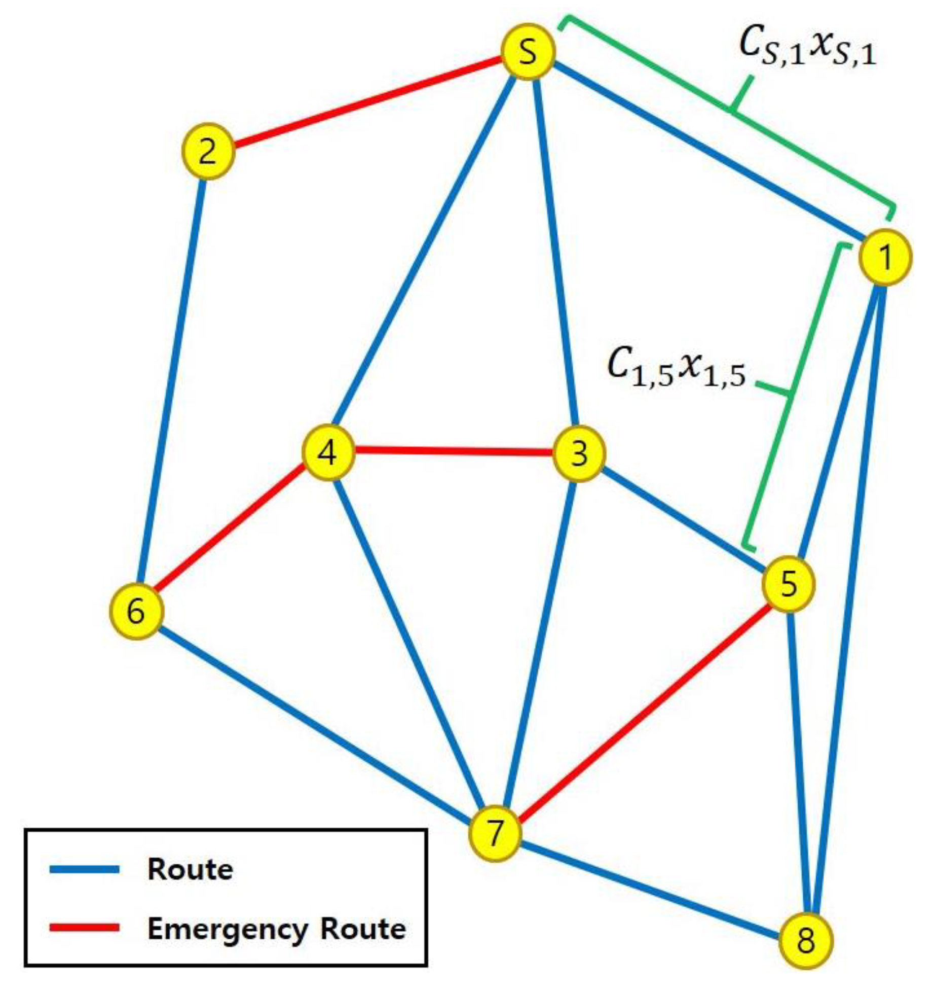
Figure 10.
Virtual road network: (a) removing nodes except for those at the end of the emergency roads; (b) calculation of the optimal virtual route.
Figure 10.
Virtual road network: (a) removing nodes except for those at the end of the emergency roads; (b) calculation of the optimal virtual route.

Figure 11.
Estimation of the optimal final route.

Figure 12.
Steps in the virtual route algorithm.

Figure 13.
Location of the starting node considering the maximum distance of 4 km from the snow-removal base derived using the Dijkstra algorithm.
Figure 13.
Location of the starting node considering the maximum distance of 4 km from the snow-removal base derived using the Dijkstra algorithm.

Figure 14.
Location information using the ID attribute.
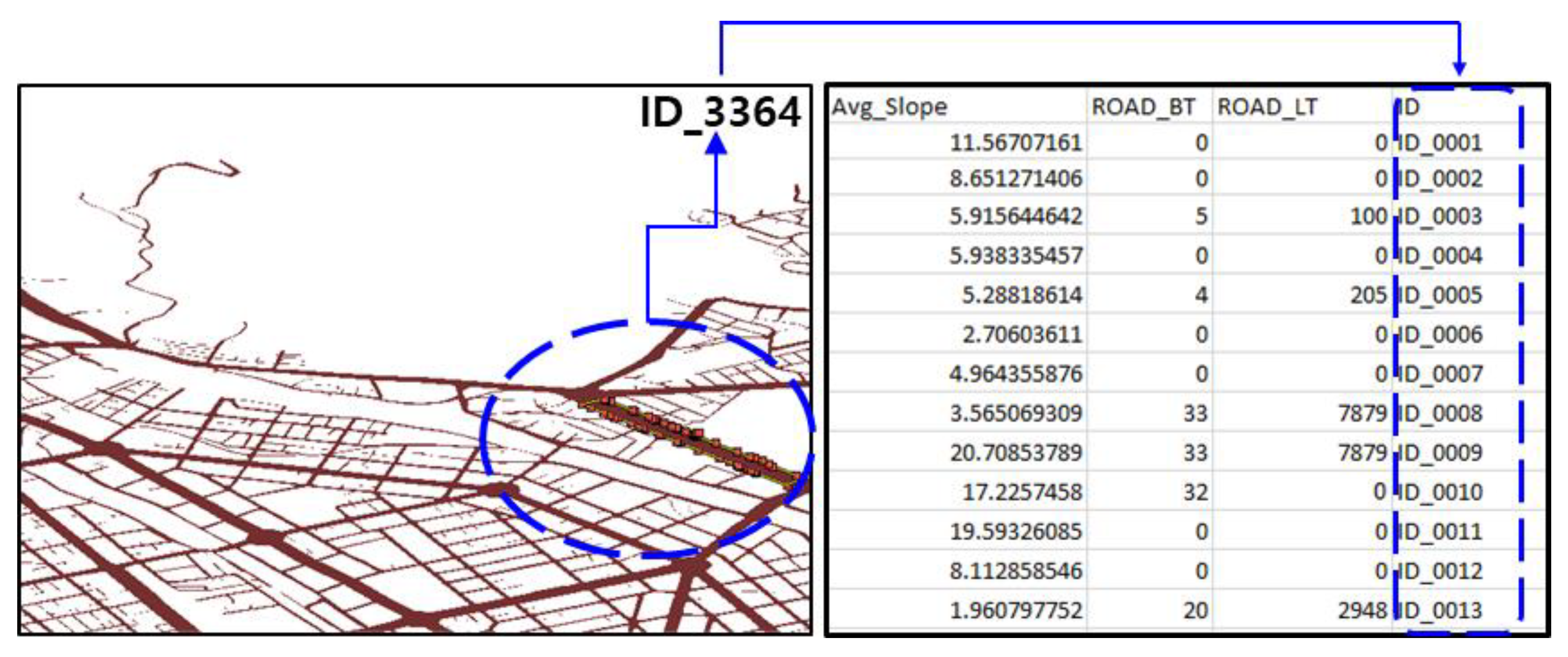
Figure 15.
Road network in the target area.

Figure 16.
The optimal virtual route: (a) shortest route network using the Floyd–Warshall algorithm; (b) estimating the optimal virtual route.
Figure 16.
The optimal virtual route: (a) shortest route network using the Floyd–Warshall algorithm; (b) estimating the optimal virtual route.

Figure 17.
Final optimal route in the target area: (a) optimal route obtained by recovering the removed nodes; (b) final optimal route considering the starting point.
Figure 17.
Final optimal route in the target area: (a) optimal route obtained by recovering the removed nodes; (b) final optimal route considering the starting point.


Table 1.
Comparison of factors affecting disaster routes and snow vulnerability.
| Disaster Route | Snow Vulnerability |
|---|---|
| Many lanes | Road direction |
| No central reserve, road shoulder, and sloping surfaces | Strong sunlight |
| Low slope | High slope |
| Roads without bridges and tunnels | Roads without vulnerable spots |
| No speed limit | Shady place |
| Low traffic volume | High traffic volume |
| Contain roadside information provision device | |
| Many links |
Table 2.
Information on the deicer sprayer [56].
Table 2.
Information on the deicer sprayer [56].
| Regulator Stage | Deicer Input (kg) | Outlet Size (mm) | Effective Spray Width (mm) | Maximum Spray Width (mm) | Spray Duration (min) |
|---|---|---|---|---|---|
| First stage | 250 | 25 | 2000 | 3000 | 60 |
| Fifth stage | 250 | 25 | 4500 | 6100 | 30 |
| Ninth stage | 250 | 25 | 6200 | 10000 | 10 |
Note: In the case of the salt sprayer, the maximum spray distance is 5 km and the maximum spray area is 22,500 m2 when spraying is performed at the first stage of the regulator for 30 min at a speed of 10 km/h.
Table 3.
Information used for the formation of a road network.
| Road Network | Target Range | Maximum Location from Snow-Removal Base (Estimated Using the Dijkstra Algorithm) |
| Target road | Roads having widths of 20 m or higher (corresponding to roads of class 2 or higher, as per the Ministry of Land, Infrastructure and Transport (Korea)) | |
| Constraints | 4% slope to ensure the necessary passing conditions for emergency roads |
© 2019 by the authors. Licensee MDPI, Basel, Switzerland. This article is an open access article distributed under the terms and conditions of the Creative Commons Attribution (CC BY) license (http://creativecommons.org/licenses/by/4.0/).
Share and Cite
MDPI and ACS Style
Park, S.H.; Jang, Y.-H.; Geem, Z.W.; Lee, S.-H. CityGML-Based Road Information Model for Route Optimization of Snow-Removal Vehicle. ISPRS Int. J. Geo-Inf. 2019, 8, 588. https://0-doi-org.brum.beds.ac.uk/10.3390/ijgi8120588
AMA Style
Park SH, Jang Y-H, Geem ZW, Lee S-H. CityGML-Based Road Information Model for Route Optimization of Snow-Removal Vehicle. ISPRS International Journal of Geo-Information. 2019; 8(12):588. https://0-doi-org.brum.beds.ac.uk/10.3390/ijgi8120588
Chicago/Turabian StylePark, Sang Ho, Young-Hoon Jang, Zong Woo Geem, and Sang-Ho Lee. 2019. "CityGML-Based Road Information Model for Route Optimization of Snow-Removal Vehicle" ISPRS International Journal of Geo-Information 8, no. 12: 588. https://0-doi-org.brum.beds.ac.uk/10.3390/ijgi8120588
Note that from the first issue of 2016, this journal uses article numbers instead of page numbers. See further details here.