Japanese Lexical Variation Explained by Spatial Contact Patterns


1
Department of Geography, Ritsumeikan University, Kyoto 623-0062, Japan
2
College of Letters, Ritsumeikan University, Kyoto 623-0062, Japan
3
Kinugasa Research Organization, Ritsumeikan University, Kyoto 623-0062, Japan
*
Author to whom correspondence should be addressed.
ISPRS Int. J. Geo-Inf. 2019, 8(9), 400; https://0-doi-org.brum.beds.ac.uk/10.3390/ijgi8090400
Submission received: 16 July 2019
/
Revised: 12 August 2019
/
Accepted: 2 September 2019
/
Published: 6 September 2019
(This article belongs to the Special Issue Historical GIS and Digital Humanities)
Abstract
:In this paper, we analyse spatial variation in the Japanese dialectal lexicon by assembling a set of methodologies using theories in variationist linguistics and GIScience, and tools used in historical GIS. Based on historical dialect atlas data, we calculate a linguistic distance matrix across survey localities. The linguistic variation expressed through this distance is contrasted with several measurements, based on spatial distance, utilised to estimate language contact potential across Japan, historically and at present. Further, administrative boundaries are tested for their separation effect. Measuring aggregate associations within linguistic variation can contrast previous notions of dialect area formation by detecting continua. Depending on local geographies in spatial subsets, great circle distance, travel distance and travel times explain a similar proportion of the variance in linguistic distance despite the limitations of the latter two. While they explain the majority, two further measurements estimating contact have lower explanatory power: least cost paths, modelling contact before the industrial revolution, based on DEM and sea navigation, and a linguistic influence index based on settlement hierarchy. Historical domain boundaries and present day prefecture boundaries are found to have a statistically significant effect on dialectal variation. However, the interplay of boundaries and distance is yet to be identified. We claim that a similar methodology can address spatial variation in other digital humanities, given a similar spatial and attribute granularity.
1. Introduction
1.1. Motivation
Historical dialect data forms a valuable part of humanities similarly to folk songs and dances, beliefs and other cultural traits. Spatial patterns present in dialects have been researched in linguistic geography for over a century, with the digital preservation and quantitative investigation of dialectal variation becoming increasingly central [1]. Further, identities are often generated by noting linguistic differences to distinguish ‘our group’ from ‘the others’, which connects dialectal variation to the human psychological needs of categorisation [2,3].
Language is constantly changing and its perceived reality at any given time is a mere snapshot, resulting from language change through preceding centuries. Divergence and convergence in language is caused by isolation and contact between the speakers [4], with language change occurring at different time scales [5]. Intuitively, a connection can be assumed between linguistic variation and the potential of contact, which is, in turn, strongly associated with spatial phenomena such as distance, facility of access by transportation, topography, and even one’s role in their social network, e.g., [6,7,8]).
Bloomfield [9] associates language change with the density of communication, which is in turn based on the mobility patterns on the macro scale. The urban hierarchical diffusion [10,11,12] is one of the models that explains the diffusion of linguistic innovations, which play a central role in language change. It assumes that innovations spread from larger populations towards smaller ones, corresponding to the mobility patterns of the population (including commute and relocation): an innovation would first be transported between cities, prior to smaller towns catching on, and finally to the countryside. Boundaries can, however, overwrite the diffusion processes by impacting the mobility patterns (e.g., by the restriction of movement, leading to isolation) and the communication norms (such as language policies), which is often the case of national borders isolating speakers of similar varieties, e.g., [13].
Japan is, due to its archipelago geography and its high proportion of rugged terrain (about 73% of its surface is mountainous or forested), contrasted by its large population concentrating in coastal areas, a typical geographic example where isolation and dense communication are present side by side. Most research on Japanese dialects focused on the linguistic relations themselves, and did not quantitatively account for the underlying potential spatial factors assumed to affect dialectal variation. With some exceptions, e.g., [14,15], quantitative studies involving aggregation of multiple phenomena across larger areas are missing.
Therefore in this article we offer a comprehensive methodology for the analysis of the spatial relations of Japanese dialects through the lens of GIScience, often criticised for its limited involvement in dialect research beyond mapping, e.g., [16], despite offering “...an articulation of spatial theory as a framework for approaching hypotheses in linguistics research” [17] (p. 28). The concept of apparent time [18,19] states that mother tongue is mostly acquired until the late teenage, after which one’s language is more resistant to change. It is therefore assumed that every idiolect bears the effect of the environment of their early life, therefore synchronic diversity can be interpreted diachronically. For the respondents of the dialect database used in this study (‘Linguistic Atlas of Japan’ (LAJ) [20]), born between 1879 and 1903, it means that their is language usage is assumed to be representative of the late 19th, early 20th century.
It is generally acknowledged that historical contact paths and isolation patterns should explain today’s language variation better than contemporary contact patterns [21]. With the support of the apparent time theory, resources in digital humanities (historical linguistic data, historical spatial networks and points of interest) and the recent surge of computational power, it becomes possible to quantitatively account for the potential contact patterns present at historical times. Our study thus embarks on explaining linguistic situation as a result of topographic and political settings at and before the time of LAJ respondents’ mother tongue acquisition, and contrasts it with the explanatory power of geographic factors that characterise more recent times.
1.2. Background
Phylogenetics has lately shown an elevated interest towards historical change in linguistic patterns, regarding, for example, language evolution [22], contact-induced change [23] and correlations with language-external traits [24]. However, historical quantitative analysis was only rarely focused on similar effects on intra-language, dialectal data [14,25].
To account for linguistic variation in space, it is common to establish a measurement of difference between locations visited in linguistic surveys, based on individual answers to survey questions. Expressing this linguistic distance between surveyed locations quantitatively is one of the most important focuses in the field of dialectometry, e.g., [26,27,28,29]. Linguistic distance is usually calculated by defining the linguistic difference between dialectal variants (different forms people use to express the same phenomenon) and aggregating theses differences for a number of phenomena between each location pair, resulting in a linguistic distance matrix [30]. The quantification of the difference between dialectal variants depends on the way these variants can be mathematically contrasted. Dialectal variants can be converted to vectors of sounds or letters, based on which Levenshtein’s edit distance [31] is often calculated in studies focused on pronunciation [32,33]. However, lexical variation is often categorical and, as sound vectors often become completely different, Levenshtein distance calculations are not always meaningful. Thus, for the lexical and syntactic level, aggregative measures based on categorical differences are often used, such as Goebl’s [34] ’Relative Identity Value’ (RIV). In a similar way, Kumagai [35] has introduced the -distance for LAJ’s lexical data, based on the number of co-occurring answers.
Recently, linguistic distances are commonly used to chart areal similarities and differences, equivalent to what has often been done in classical dialectology by searching for overlapping dialectal boundaries that separate answer variants of different phenomena, from as early as 1898 [36,37,38]. The areas found were often classified as dialect areas, although aggregative studies rarely reproduce dialect areas with sharp boundaries, and thus argue for continua in the distribution of dialectal variants, cf. [39]. Embleton [40] introduced multidimensional scaling (MDS), a dimension reduction technique, into dialectology, to reduce large dialectal matrices to a three-dimensional space, and associated the three components of the RGB colour space with these three dimensions, to show the continuous nature of transitions between dialect areas. Since then, MDS has become a common tool for dialectometric visualisations [28,33,41,42], showing the association across localities with regards to a multitude of phenomena. Many contemporary dialectometric studies use principal components analysis (PCA), e.g., [43], or factor analysis, e.g., [44,45,46], to detect linguistic items showing similar geographical patterns. Besides, hierarchical cluster analysis is often used for finding linguistically similar locations [43,47,48]. The mapped results of such analyses are often used to validate dialect area maps produced by the classic “isogloss bundling” method [36,37,38].
Once linguistic distances are calculated, it is common to attribute them to some (geographical) measurements that account for the possibility of language contact. Holman et al. [49], inspired by population genetics [50], explicitly associate the concept of ‘isolation by distance’ among the world’s languages with the situation faced by dialectology. The axiomatic role of geography structuring language, phrased by Nerbonne and Kleiweg [51] (p. 154), which practically describes spatial autocorrelation in dialectal variation, was tested in numerous studies, e.g., [15,21,26,41,52,53]. Nerbonne and Kleiweg’s postulate, “geographically proximate varieties tend to be more similar than distant ones”, is, in effect, the linguistic adaptation of Tobler’s first law of geography [54].
The role of space, practically accounting for the potential linguistic contact between locations, has mostly been expressed by Euclidean distance, e.g., [26,52,55]. Séguy, who initiated the research of relating linguistic distance to geographic distance [26], observed a logarithmic relationship, which is since then assumed to be present between the two types of distances. Gooskens [21] was the first to operationalise the possibility of contact using contemporary and historical travel times. Since then, several studies have attempted to explain dialectal variation using geographic distance measures deemed to be more powerful for expressing a possibility for dialectal contact than Euclidean distance. Inoue [56] used distance along railways in Japan, Stanford [57] tested ‘rice-paddy distances’ in a clan-based society, Lameli et al. [58] associated dialect similarity to trade frequency in Germany and Derungs et al. [25] used least cost paths in mountainous areas of Switzerland.
Although Gooskens [21,59] and Jeszenszky et al. [53] confirmed the superior explanatory power of travel times, multiple studies for different languages [52,57,60] have found that travel times are not a better predictor for dialectal variation than Euclidean distance. Regarding historical contact, Huisman [14] showed that mainland Japanese displays an isolation-by-distance pattern, while Ryukyuan varieties display a typical isolation-by-colonisation pattern. Sociodemographic factors also play an important role in language variation beside spatial ones, increasingly affecting patterns in society, especially with mobility patterns changing. Mobility and commuting patterns are claimed to have a role in the diffusion of innovations. The original model accounting for this effect similar to gravity was worked out by Trudgill [11] to correspond to the potential of linguistic interaction between communities, and it has been popular in dialectology, e.g., [25,52,61].
Due to their potential isolating effect, coincidence of dialectal boundaries with political and natural borders has often been tested, e.g., [62,63,64]. Derungs et al. [25] tested the impact of administrative and cultural boundaries on dialect variance using spatial autoregressive models. In relation to Japonic languages, Lee and Hasegawa [8] showed that ocean straits between Japan’s islands act as a barriers that promote diversification. Nevertheless, effects of administrative boundaries within mainland Japan have not been quantitatively tested for their isolation role in language.
Despite the fact that Japanese dialects are among the most thoroughly researched ones, the explanatory power of geographic factors on linguistic variation has not been researched until lately [14,15]. Japanese dialectology until recently, similarly to traditional dialectology in general, was involved mostly in qualitative studies of characterising individual linguistic phenomena, e.g., [65,66,67], and quantitative studies involving aggregation of multiple phenomena based on surveys, but excluding geostatistical analyses. The latter line of research is exemplified in Tanaka’s work [68], tracking the diffusion of Standard Japanese lexical features from the former and present capitals (Kyoto and Tokyo). Since the end of the 19th century in Japan, the official language policy enforced using Standard Japanese, based on the variety spoken in Tokyo (called Edo before 1869), in all official situations and in schools. Since then, due to the low prestige associated with non-standard language, usage of Japanese dialects has been dwindling and converging to the Standard, retaining less regional variation. Nevertheless, regional differences in language variety keep enjoying popular interest and strengthen the feeling of belonging and group formation in Japan, similarly to dialects in other countries. Although several different research directions were explored using the data from the Linguistic Atlas of Japan (LAJ) and other dialect surveys, the lack of digitised data hindered very profound discoveries in many of these directions [35,69,70,71,72,73,74,75].
Some peculiarities are important to note about the language landscape of Japan. Traditional dialectology and computational approaches have proven the split between Japanese and Ryukyuan, the variety of Okinawa prefecture in southern islands, often considered separate languages [14,76,77]. Due to this, Okinawan varietes are outliers in the LAJ as well. Besides, the northernmost large island, Hokkaido is, on the one hand, less densely populated than other parts of Japan and, on the other hand, has less distinct dialects because of its more recent large-scale settlement (starting at the end of the 19th century, mainly from Honshu), resulting in more mixed and standardised varieties.
The data used for this research stems from the digitised LAJ survey data (LAJDB) [75]. LAJ was produced at the National Language Research Institute (NLRI), today called National Institute of Japanese Language and Linguistics (NINJAL), presenting the recorded material of a large-scale survey conducted between 1957 and 1965. Throughout Japan, 2400 localities were surveyed, interviewing one male respondent, born between 1879 and 1903, at each locality. The survey locations are mapped in Figure 1, together with the most important regions of Japan, the main islands, showing the main roads.
1.3. Aims of the Research
In this study, we investigate the driving factors of dialectal variation and quantify contact between communities at a historical scale making use of the potential of theories of GIScience and variationist linguistics, and tools used in historical GIS. We identify the missing locality level dialectometric analysis of Japanese dialect data as the main research gap and focus on providing a comprehensive methodology to address it.
We establish a linguistic distance between localities based on the digitised LAJ data (termed LAJDB). We perform an overlap analysis across the variants used throughout Japan, in search of spatial clusters without taking space explicitly into account. Besides, using multidimensional scaling (MDS) on the linguistic distance calculated, we provide a contrast to classic dialect maps often showing the presence of dialect areas and by sharp borders, e.g., [78].
Due to the fact that linguistic variables chosen for dialect surveys usually exhibit spatial variation, we may assume that spatially autocorrelated geographic factors explain a considerable proportion of the variation in our survey data as well. We are motivated to research the historical contact potential by the assumption that preceding environmental settings impact language variety, in relation to the concept of apparent time. Potential contact might depend on accessibility rather than just distance, especially in case of an archipelago nation such as Japan, inviting the question of how to best estimate contact in such a scenario. Because of the regional differences in Japan, as in the case of the Ryukyu Islands and Hokkaido, we employ a local approach beside performing global calculations.
We build the following models:
- A series of models estimating contact potential:
- -
- before the time of infrastructural development, using network of least cost paths based on digital elevation models (DEM),
- -
- at present, using today’s road network for calculating travel distances and travel times
- -
- independent of time, using the great circle distances between localities.
- A model estimating the potential influence between communities based on their population density and an inverse-distance association similar to the law of gravity.
- Finally, we test the separating effect of administrative boundaries, on the one hand the administrative system of domains (Japanese: han) used in the Edo-era (1603–1868), which are deemed to have affected the language variation before the LAJ respondents’ age of mother tongue acquisition, due to restriction of free movement [79], and on the other hand their modern counterpart, the prefectures (Japanese: ken).
The methodologies presented in this work contribute to the characterisation of the Japanese lexical dialectal landscape. The methodology accounts for geographic factors in a differentiated way, and revisits associations among linguistic variables and the spatial patterns of their variants through quantitative analysis. Based on this, the conventional dialect area formation theories of Japanese (often coercing dialectal boundaries onto natural and man-made boundaries, much like the perception of laypeople would delimit continuous variables) can be revisited. Further, the models worked out for this study can be easily scaled to data in other languages or other data in digital humanities with similar distribution and granularity.
2. Materials and Methodology
As this work conducts a comprehensive quantitative analysis of language data contrasting it to several different spatial factors, the structure of the present section needs some explanation. First, we introduce the LAJDB. Second, we present the data processing steps and the related overlap analysis. Third, we detail the design of the linguistic distance measure. Fourth, we account for the spatial association of linguistic distance by MDS. Fifth, we walk through the different analyses implementing the distance-based spatial models described in Section 1.3. We will use the generic term ’spatial distances’ for the measurements in these models which estimate contact potential based on spatial factors. Finally, we present the methodology for testing the impact of administrative boundaries. Similarly, in Section 3 the results of each analysis and their interpretation is presented sequentially, followed by a comprehensive concluding section.
2.1. Dialect Data: The Linguistic Atlas of Japan
This study uses digitised and publicly available data from the LAJDB [75] (For a comprehensive English language summary of LAJ and LAJDB see [75].). LAJ is a dialect atlas based on a survey conducted from 1957 to 1965 by the National Language Research Institute (NLRI), the predecessor of NINJAL. The atlas was published in six volumes between 1966 and 1974. The atlas contains 285 questions (termed variables in this work), mostly about lexical variation (the linguistic term for variation in vocabulary), including common nouns, verbs and adjectives. 2400 localities were surveyed by 65 fieldworkers by means of personal interviews. At each location, one respondent (a male in almost all cases) was interviewed. The respondents were born and grew up at the survey location or lived there without interruption from the age of 3 to 15 [75]. Most respondents of the LAJ can be described as “NORMs”, i.e., non-mobile, old, rural males [80], which in dialectology translates to the research aims of such surveys finding the “oldest” possible, “authentic” dialectal forms present, sometimes called the “base dialect”. Due to the sampling strategy of LAJ (one NORM per locality), the variation within localities is hidden. However, in some localities, two or more linguistic forms of some linguistic variables were recorded from the same respondent. the fact that approximately 80% of all localities were agricultural communities [20] also shows that NLRI wished to record a variation as little impacted by urbanisation and standardisation as possible. About six localities are surveyed every 1000 km, except for Hokkaido. Figure 2 shows LAJ map nr. 182, presenting the distribution of the variants used to express ‘corn’ or ‘maize’.
We used 37 variables from LAJDB, available online (www.lajdb.org) at the time of the research. The majority of these variables focuses on basic vocabulary in relation to body parts, weather and time, animals and plants, and levels of kinship. We identify this focus as a risk factor for our results being representative of the LAJ.
According to the concept of apparent time, we infer the potential contact patterns that might have shaped the dialectal landscape before and at the time of the respondents’ mother tongue acquitisition. Apparent time constructs were used to infer the synchronic manifestation of a language change in progress for various levels of linguistics [81,82]. It is claimed, however, that rates of change vary by linguistic level (e.g., lexicon, pronunciation, morphology, syntax), with lexicon, i.e., the function of words, their semantics and meaning, with a higher rate of change compared to other linguistic levels [83]. We identify this as a potential risk for our apparent time approach.
2.2. Categorisation of the Dialect Data: Overlap Analysis
We start the dialectometric analysis by discovering the associations across the dialectal variants in the 37 variables. Doing so we aim to find out whether certain variants are used together, but without the bias usually present in traditional analyses, i.e., the map comparison dialectal analysts usually do in search of individual variables’ similar patterns. Lexical variation present in certain linguistic items can be immense, and this is also recorded in LAJDB. To reduce variation, we categorise the answer variants for each variable based on the original LAJ maps (Original LAJ maps of the variables in LAJDB are available online: https://mmsrv.ninjal.ac.jp/laj_map/). In LAJ maps, variants’ symbols are grouped together based on phonetic similarity, historical relations and semantic categories (see the map legend example in Figure 3). Using the groupings present on the maps, the number of answer categories is reduced from approx. 10-500 to 3-15 per variable. We term the resulting categories variant categories.
To measure the overlap of usage between two categories, we use a measure of association similar to the Jaccard index, as we calculate the intersection over the union of the users of the variant categories. For a pair of variant categories, we take the number of localities where the variant categories are used concurrently (overlaps) and divide it by the number of localities where only one of the variant categories is used (divergences). A similar approach is present in previous research e.g., Uiboaed et al. [84], who used the statistical ordination method correspondence analysis (CA) in dialectology, but for finding associations across localities, rather than dialectal variants.
Based on the correspondence matrix of variant categories, we show a graph of associations for each variant category with all others, independent of geography, created using the R package qgraph [85].
2.3. Linguistic Distance: Quantifying the Dialect Variation across Localities
Based on the variant categories, we calculate linguistic distances for each pair of survey localities. Our linguistic distance measure is similar to the NC-measure of Kumagai [75] and the RIV-values of Goebl [34]. For a locality pair, our measure is defined based on the sum of differences for each of the 37 variables. In turn, the difference for each variable between localities i and j also takes into account differences within a variant category (see also Figure 4). If for a linguistic variable all answers in localities i and j are in different variant categories, then a linguistic distance of 1 is assigned to this locality pair for this variable. If i and j has answers in the same variant category, but not exactly the same variant, the linguistic distance grows by a flat rate of 0.2. Finally, if the answer(s) in i and j for this variable completely overlap(s), the linguistic distance does not grow. The linguistic distance between localities i and j is then summed:
where n is the number of variables with answers from both respondents (both localities), is the grade of divergence or correspondence for an individual variable, regarding localities i and j. For a forged example, see Figure 4.
For linguistic distance calculations missing answers are not taken into account. In case answers in i and j are in the same variant category, the answers might be fairly similar to each other or wildly different. Variant categories impose sharp boundaries in an otherwise fuzzy and diverse continuum of lexical variation, often diverging based on the pronunciation of the linguistic item. Although for pronunciation the Levenshtein distance is often used in dialectology for defining the distance between two vectors, e.g., [32,33], we may not use this approach because of the variants that are categorised together due to a sound of interest, however completely diverge, e.g., ‘nanmai’ and ‘banbarakibi’ in the example variable in Figure 3). Two variants in the same variant category can also be a pair of compound words with the two parts swapped. the histogram of variant occurrences in a variant category, however, has a long tail, similar to a Zipf-curve [86] (p. 384). In most cases this means that the majority of answers in i and j that fall into a certain variant category are actually also the same variant. We decided for a flat rate of 0.2 when noting linguistic distances within a variant category because of such discrepancies within variant categories. We tested the effect of flat rates’ from 0.1 to 0.5 on the resulting linguistic distance and the correlation coefficient always stayed above 0.97.
Having created the linguistic distance matrix, the linguistic distances can be mapped from any of the 2400 localities.
2.4. Discovering the Spatial Association of Linguistic Distance by Multidimensional Scaling
Calculating the linguistic distance matrix allows the discovery of the encapsulated spatial association. As we created a distance matrix based on the 37 variables, multidimensional scaling (MDS) can be performed directly on this 2400 × 2400 distance matrix, containing the continuous values for linguistic distance. Practically, MDS reduces the extent of a multidimensional point cloud into a space as low-dimensional as possible (most research reports two or three, similarly to Principal Component Analysis). “Each dimension extracted by multidimensional scaling represents a specific pattern of regional variation and can thus be interpreted in isolation. However, it is more common to display two or three dimensions simultaneously” [87] (p. 257). In our case, clusters of data points in a three dimensional space can be interpreted as localities (actually respondents) similar to each other with regards to the multitude of dimensions. Assigning the values along these dimensions to RGB (Red, Green, Blue) colour values, the resulting colours can be used to find spatial associations when the locations are mapped. As a consequence, MDS supports the investigation of dialect area formation, a central topic in linguistic geography. Moreover, dialect areas often defined by the traditional methods of searching for ’isogloss bundles’ can be revisited based on a larger number of variables.
2.5. Estimating the Dialect Contact Potential
In effect, our models in Section 1.3 test correlations of linguistic distance with the different ’spatial distances’ (as estimations of contact potential) at the global level and in different functional subsets, the main islands of Japan, using Pearson’s product-moment correlation. As logarithmic relationship with geographic distances was commonly found in previous research [26,30,39], we perform tests with the logarithm of the explanatory variables as well. Statistical significance of the differences between the resulting correlation coefficients is tested by means of a z-score suggested by Meng et al. [88], implemented in R package cocor [89].
2.5.1. Great Circle Distance
To account for the possibility of contact between communities, most dialectometric research, by default, uses the linear or Euclidean distance. therefore we also use the Euclidean distance as a baseline for testing the explanation power of other distance-based explanatory variables. We obtained great circle distances (GCD), i.e., Euclidean distances on the surface of Earth, using the ’fields’ package [90] in R, for each locality pair. We perform correlation tests with the linguistic distances and GCD, together with their logarithms. The distribution of GCD has a strong positive skew with the largest distance being 2964 km between Western Okinawa and Northern Hokkaido.
2.5.2. Travel Distance
GCD might overestimate the potential contact between communities, as contact paths are seldom straight due to obstacles in the landscape, such as mountains, rivers or lack of roads. Using the ArcGIS Data Collection Road Network in Japan (state of 2016), we calculated shortest travel distances (TD) for locality pairs in ArcGIS with the help of arcpy scripts. The resulting TD matrix has limitations, however, as it only contains values for locality pairs that are reachable on land, with missing values accounting for 29.27% of all locality pairs. This leaves little results for Okinawan islands and other smaller islands not connected to the main islands Honshu, Kyushu, Shikoku and Hokkaido by bridges. Shikoku and Kyushu are connected to Honshu by road bridges, but Hokkaido is not. The network available did not include ferry routes, therefore giving unrealistic contact patterns in relation of locality pairs on Kyushu, Shikoku and Honshu as well, practically moving the agents through bridges, even if a ferry was available.
The distribution of TD has a positive skew with the largest distance being 1999 km within the connected islands of Honshu, Shikoku and Kyushu. However, due to the presence of large distances and with a large number of locality pairs taken into account, the difference between GCD and TD is assumed to level out. Because of this we expect the difference in their explanatory power to be more meaningful in the regional subsets.
2.5.3. Travel Times
Shortest paths in networks are, however, not always the fastest paths, as they do not take into account the quality of the roads and the permitted speed. Therefore the time necessary to reach a certain point is hypothesised to be a better estimation for potential contact between communities. Gooskens [21,59] and Jeszenszky et al. [53] tested the correlation of travel times and Norwegian and Swiss German dialect differences, respectively, and found that historical travel times explain more variance in the linguistic distance than contemporary travel times. Using Open Source Routing Machine (OSRM) through its implementation in R (package ’osrm’) [91], we obtained present day travel times (TT) by individual transportation. OSRM sends batched requests to the Open Street Map (OSM) routing client and gets back travel time values. As OSM navigation takes ferry routes into account, the resulting TT matrix has a missing value rate of only 3.14%. However, ferry connections towards islands in Western Okinawa are missing. Besides, as OSRM does not incorporate common modes of transport faster than car transport, such as airplanes and the shinkansen high-speed railway lines of Japan, TT obtained might underestimate the present day contact potential between localities.
Nevertheless, this TT matrix represents contact paths some 50 years after the dialect survey and more than a 100 years after the time of the respondents’ mother tongue acquisition. We might assume, however, that with the increasing speeds in the system, the proportions in travel times have not significantly changed during these times, disregarding high-speed connections, which our OSM-based model also lacks. The distribution of TT has a strong positive skew with 94% of the values under 36 h.
2.5.4. Least Cost Paths and Hiking Times
As it is commonly assumed that historical contact patterns would explain today’s dialectal landscape more, we aimed to model the potential contact paths in Japan before the infrastructural boom brought by the industrial revolution. In Japan the industrial revolution began in the 1870’s, not much before the LAJ respondents’ mother tongue acquisition. Therefore we assume the effects of ’intact’ relief and environment to have had a substantial effect on the dialects surveyed. Our assumption is that least cost paths, the most natural paths of contact between communities, were predominantly unchanged for centuries before the industrial revolution and over land they would substantially depend on relief. We also assume that the first paved roads and other measures for speeding up transportation (earliest railways) were implemented along least cost paths. Our model is based on the 10 m resolution digital elevation models (DEM) in the Fundamental Geospatial Data (https://fgd.gsi.go.jp/download/ref_dem.html) provided by the Geospatial Information Authority of Japan, which we resampled at 100 m resolution.
Using Tobler’s hiking function [92] (Equation (2)), which defines average walking speed as the function of the terrain’s slope, we calculated the “hiking times” along the least cost paths for all locality pairs, similarly to [25,93]. With its peak walking speed for slight downward slopes, the function is asymmetrical, marked with a shift of 0.05 in the exponent (the shape of the function is shown in Figure 5):
where V is the velocity of walking and S is the slope value in radians.
This asymmetry means that in most cases the resulting least cost paths and subsequently the hiking times differ depending on the direction of the path calculated between localities. As contact between any communities is bidirectional, for each locality pair we take the mean of the resulting hiking times along the least cost path.
To calculate least cost paths between localities separated by sea (i.e., where a path over a DEM is not available), we allowed sea navigation. The speed of sea navigation was defined as 2.5 times larger than land movement on flat surface, to match the premise of pre-infrastuctural contact paths on land with that of sailing median speeds before steamboats. The speed was established based on Casson’s calculations [94], who gathered travel speeds of the Mediterranean in the antiquity. This relatively slow speed is an average, taking into account favourable and unfavourable wind conditions. This slow speed also balances to a degree the fact that the agents in the model start sailing at the exact time they reach a port, which would be unimaginable in reality. To restrict the movement as much as possible to plausible shipping routes we restricted “sea entry” to ports that were important in the Edo-era (1603–1868), based on data from Saito’s research [95]. To be able to reach all localities, including those on smaller islands, further “ports” were added to the model. We allowed only near-shore navigation, limiting the model’s inclusion of sea to 50 km off the coast. Besides, we used the natural state of Japan’s coastline, before the land reclamations around port cities took place mainly after WWII. ArcGIS 10.6 and arcpy were used for the model calculations. the crucial location of ports from the point of view of potential contact is visible in Figure 5. Because of some obvious limitations of the model, such as the lack of land cover, the 100 m resolution and not taking fatigue or constant availability of ships into account, results from our model should be taken with a grain of salt.
As we allow for sailing beside moving in the DEM, there are no points pairs in our model that are not connected. In the remainder of this paper, we will term the measurement resulting from this model hiking time (HT). Of all our explanatory variables, the distribution of HT has the weakest positive skew, with a median in HT around 90 h and maximum of 384 h.
2.5.5. Linguistic ’Gravity’ Index
To estimate the probability for actual contact across localities beyond accessibility, we calculated a gravity-like index, estimating the potential ’interaction’ between communities to which survey locations belong, based on their geographic distance and their population densities. It is expected that more populous communities would interact more with each other, even if they lie farther away. Besides, such ’gravitational’ model is assumed to align with commuting and other communication patterns between smaller and larger settlements, i.e., villages would have more interaction with a nearby city than with the surrounding villages. the original of this model was worked out by Trudgill [11], and the resulting index is often called Trudgill’s linguistic gravity index (TLGI). In Szmrecsanyi’s words the inverse-square law of gravitation “postulates that the interaction between two dialects decreases with increasing geographic distance but this effect is counterbalanced by larger speaker communities” [52] (p. 222). Based on the Newton’s law of gravity, TLGI is formulated as Equation (3):
where M is the index of potential interaction (TLGI), P are the populations of the two localities in question and D is a distance measure between them.
Owing to the characteristics of the Japanese administrative and census system, data available about population is suboptimal. There is no direct data available about each settlement and thus, village population. However, data is available in the form of a census grid with several kinds of data about the local population merged into 1 km grid cells. We used population data from 1975 and 2005 from this gridded census data. The year 1975 is the closest available to the time of the survey and 2005 is closest to the peak of Japan’s now declining population. For each LAJ locality, we considered the intersection of the population in grid cells with a 2.5 km radius buffer as the local community. Incidentally, in LAJDB, the survey locations’ coordinates are snapped to the corners of the 1 km grid census grid, for privacy reasons. Thus for each locality, the same amount of grid cells are considered. This way the P weights in our model actually correspond to a neighbourhood level population density. On the downside, the distribution of population assigned to our localities does not reflect the actual population present in the municipalities, especially regarding metropolises. Although the actual population would be in the millions in several municipalities and in the 100,000s in dozens of municipalities, our P weights never go over a million and they are over 100,000 in the top one hundred localities, most of which pertain to areas of metropolises. This is thought to skew the gravitational force metropolises exert over long distance. However, the locally stronger gravity (due to several localities falling into today’s metropolitan areas) might better reflect the communication patterns characteristic of the Meiji-era.
As GCD was available for all locality pairs, we used it as the distance measure in TLGI.
A logarithmic correspondence is expected between the linguistic distance and Trudgill’s linguistic gravity index (TLGI).
The gravity index is extremely skewed to the right with most localities incapable of direct contact (with TLGI value converging to 0) and nearby populous localities with a very strong impact on each other. The latter are basically the survey locations in metropolitan areas where the respondents practically belong to the same city rather than their 2.5 km neighbourhood, and thus their dialects should theoretically be the same. While the largest index values are in the thousands, 99% of the values stay under 0.2.
2.6. Explaining Linguistic Variation through Administrative Boundaries
We tested the separating effect of administrative boundaries of domains and prefectures, described in Section 1.3. These boundaries restricting the movement of their inhabitants is claimed to be one of the key factors in the formation of the latest Japanese dialects [79]. We test the effect of boundaries of 68 domains at the time of their abolition in 1868 on the lexical variation, together with the effect of prefectures. However, the boundaries of the 47 prefectures follow domain boundaries very closely and are virtually unchanged since 1888. It can be assumed that those domain boundaries were kept as prefecture boundaries that denoted an important isolation factor anyway.
The effect of administrative boundaries was analysed using the non-parametric Mann-Whitney U test (also known as the two-sample Wilcoxon rank-sum test). The null hypothesis is that both samples are from the same population and the U test determines whether two independent samples were selected from populations with the same distribution. Unlike the t-test, the U test does not require the assumption of normal distributions and unlike p-values, the U test is not affected by sample size. We perform a subsequent Vargha-Delaney effect size test [96] on domain and prefecture boundaries, and report the probability that a value from one group will be greater than a value from the other group, that is, we show the stochastic dominance of one group, when present, unaffected by sample size [97]. The groups used in the tests are the following:
- Both localities are located in the same domain or prefecture (termed ‘within’ group) and
- the localities are separated by domain or prefectural boundaries (termed ‘separated’ group).
This grouping fulfills the requirement of the U test, assuming that the observations are independent. A significant result of the U test would suggest that the values for the two groups are different and the linked Vargha-Delaney A value shows the direction and probability of the difference.
The tests are done for each domain and prefecture separately and also as an aggregate. In order to compare the effects of domains and prefectures, we performed the tests for prefecture boundaries in the area covered by domains in 1868 (practically excluding Hokkaido and Okinawa, which were incorporated later into Japanese administration). Due to their more historical role, we assumed the domain boundaries to have a larger effect on the variation, resulting in larger linguistic distances for the group ’separated’ by boundaries.
As Japan’s area is large, its administrative regions vary in size greatly, and internal migrations assumed lower in volume before and at time of the of the LAJ respondents’ mother tongue acquisition than today, we performed the above tests with various distance cut-off measures. That is, we restricted the locality pairs considered in the tests to various distances, between 50 km and 200 km. This assumes that effects of isolation inflicted by the boundaries would manifest themselves with a relatively small distance cut-off already.
3. Results and Interpretation
3.1. Association Across Linguistic Variants Disregarding Space
The association graph in Figure 6 visualises the variant categories that are used together in the survey locations, and the strength of the connection, proportional to the Jaccard index. Parallel to analyses in traditional dialectology delimiting dialect areas based on isogloss bundles, e.g., [36,37,38], this overlap analysis shows the degree to which dialect areas can be discovered based on the 37 lexical variables considered, but, importantly, independent of geography. Having no spatial association thus means that our overlap analysis avoids the spatial bias that is present when creating isoglosses by drawing lines on maps. the strongest connections ultimately mean exclusive overlap of the areas covered by the variants in question. The network visualisation in Figure 6 uses the Fruchterman-Reingold algorithm, which also conveys that the positions or distances of nodes are not supposed to be spatially interpreted [85,98]. The color saturation and the width of the edges corresponds to the absolute weight and scale relative to the strongest weights in the graph.
In Figure 6, two main clusters can be identified, with the association strength gradually fading out around their centres. The larger cluster is associated with the Standard Japanese variants, usually found spread across large areas on the main island Honshu. The more central the node’s position within such cluster, the more the variant category overlaps with others, signaling their ubiquitous distribution. The spatial relations of such variant categories can be verified on LAJ’s individual variable maps. The smaller cluster on the right is associated with variant categories used in Okinawa, hinting at the fact that variants used here usually do not overlap with the variants used in Honshu, Shikoku or Kyushu. The close-knit cluster lets the observer associate on a high grade of exclusivity, except for its top right part, which represents variant categories used on the Sachishima-islands, the westernmost island group in the Ryukyu Islands, with what appears to be a distinct dialect based on our data.
Based on the 37 variables however, the classic of dialect areas’ definition established using isogloss bundles cannot be proved or disproved. On the one hand, even the close-knit clusters of overlapping variant categories include only a few of the variant categories rather than one variant category from most variables. On the other hand, the variant categories in the largest cluster are used throughout vast areas in Honshu, a finding which would not qualify to building dialect areas. This pattern invites the question whether the linguistically opposing concept, the dialect continuum theory can be warranted based on the data available. This interpretation is connected to analysing the results of the MDS.
3.2. Linguistic Distances Mapped
Calculating the linguistic distance matrix allows producing maps with different reference locations, i.e., presenting linguistic distances in reference to certain localities. This kind of visualisation goes back to Goebl’s dialectometry [34,99]. Figure 7 maps the linguistic distance from the following six localities: the north of Hokkaido, a rural site in Aomori prefecture in the north of Honshu, Tokyo, Kyoto, Matsue city in Shimane prefecture in the west of Honshu, and Okinawa’s capital city, Naha. Tokyo (formerly Edo) and Kyoto are the present and the past capitals and cultural centres of Japan, and therefore thought to have affected the language of the whole country by being the starting points of the (hierarchical) diffusion for many linguistic innovations [74,100,101]. Aomori in the northern extremes of Honshu is far away from both capitals, and as such, it is associated with preserving dialectal features less affected by standardisation. Matsue is the centre of the so-called Umpaku dialect area which has a unique historical aspect. Hokkaido was settled by the Japanese primarily from the end of the 19th century, exactly when the respondents were acquiring their mother tongue, from different parts of Japan but mostly the Tohoku (NW) and Hokuriku (the western shore of central) areas in Honshu. Because of this, the language history is not deep and respondents are assumed to inherit their ancestor’s language leading to a dialectally mixed area with Standard Japanese having gained ground more easily. It is not attested in our 37 variables whether the antecedent Ainu population of Hokkaido affects the variants used. Lastly, Okinawa as an archipelago used to be a semi-independent kingdom mostly isolated from imperial Japan until incorporated as a prefecture in 1879, also shortly before the LAJ respondents’ mother tongue acquisition. Because of the historical isolation, vast differences are expected between Okinawan and “mainland” varieties.
In general, Figure 7 shows that the closer a locality is to the reference locality, the smaller their linguistic distance, but Okinawa tends to show uniformly larger linguistic distances, while Hokkaido’s localities are never extremely different from the reference localities. The northerly Hokkaido locality seems to be lexically close to various areas, attesting a mixture of dialects or the degree to which Standard Japanese is used in different parts of the country. Interestingly, the north of Honshu (Aomori, Tohoku) are some of the linguistically most different areas from this locality. The Aomori locality seems to only have a small area of linguistic similarity with most of Honshu, Kyushu and Shikoku being different. At the same time the southern tip of Hokkaido seems more similar, which hints on the language connection present throughout history. Linguistic distances to Tokyo (the birthplace of Standard Japanese) tend to be smaller throughout Honshu, and most Hokkaido localities express a similarity with it. The largest distances are found in the north of Honshu (Tohoku) and the south of Kyushu, the geographically farthest areas. Kyoto, as the former capital is expressly similar to its surroundings, in the so-called Kinki area, with its similarity gradually fading away by distance and levelling to the highest differences in the north of Honshu and south of Kyushu. Interestingly, similarity between the Tokyo and Kyoto area is not salient in these maps, based on our set of variables. the area looking similar to Matsue spreads farther away than Kyoto’s and also looks concentrical, with the exception of Hokkaido. Okinawa is, finally, uniformly different in all maps with reference points on the larger islands. Its own reference map centred in Naha, the capital city of Okinawa shows extreme difference with all other provinces of Japan and even in the Okinawa prefecture itself, the Sachishima-islands in the west present a relatively large difference.
Based on the linguistic distance matrix, for each locality an average linguistic distance can be calculated to all other localities by taking the mean of each matrix row. Mapping these average values, used also in [53], adds a technique to Nerbonne’s inventory of mapping aggregate variation [28]. The resulting map in Figure 8 can thus be interpreted as a degree of overlap between the locally used lexicon and all other localities’ lexicon. Importantly, similar colours do not correspond to linguistic similarity, but to mean difference from all localities being similar. Although the lexical distance is calculated based on only 37 variables, the map shows several interesting points. The most conspicuous interpretation of the map is that Okinawan varieties are the most different from all others on average, as expected. The localities closest to all other sites are found on Hokkaido, attesting the mixed nature of the local varieties. In Honshu the area spanning from North of Kanto (the area containing Tokyo) to the West of Kansai (the area encompassing Kyoto, Osaka, and the cultural centre of Japan before the Edo-era) is a seemingly average area, fading out into the extremes of the three main islands: to the north of Honshu, and south of Shikoku and Kyushu.
3.3. Dialectal Variation in Space
Having performed the multidimensional scaling (MDS) on the 2400 × 2400 linguistic distance matrix, we can represent the dialectal variation in a three dimensional space, which is readily interpretable. These three dimensions are assigned to the RGB colours. Interpreting the similarly coloured clusters and spatial areas similar in either the 3D plot or the map in Figure 9 is practically equivalent to finding similar survey sites with regards to all 37 variables and therefore to accounting for dialect areas. Figure 9 excludes the Ryukyu Islands (containing Okinawa) due to their large linguistic distance from all other parts of Japan. Despite the removal of the outlying Ryukyu Islands, no genuinely isolated clusters are visible in the 3D plot. Although contrasting colours and certain central areas can be identified in the map, such as the northern part of Honshu, the Kanto area centred around Tokyo, or the south of Kyushu, the transitions in between remain gradual, attesting for the theory of dialect continua. As expected, Hokkaido’s localities seem to be mixed and brownish in colour, which indicates equal mixture of RGB colours and thus centrality. In essence, there is a contrast between the MDS map based on the 37 variables at hand, and the classic area formation map of Japan, e.g., [78]. The boundaries of dialect areas usually bordered by sharp lines can be considered to be a representation of some core varieties based on the MDS map, painting a fuzzier picture of the transitions present between these cores.
An additional MDS conducted only on the Ryukyu Islands revealed that isolated clusters can be found based on the 37 variables, despite the small subset. Having found four isolated clusters—namely, from West to East, the Yaeyama Islands, the Miyako Islands, the Okinawa Islands (containing the capital), and the Amami Islands (belonging to the Satsuma domain of South Japan since 1624, rather than the then Ryukyu Kingdom)—hints on the historical isolation not only between the Ryukyu Islands from mainland Japan, but also within itself.
3.4. Correlations with Spatial Measurements
We calculated several values estimating the potential of dialect contact across localities in the LAJ. For the continuous values, we built spatial distance matrices similarly to the linguistic distance and for all matrix pairs, Pearson product-moment correlation was calculated. Figure 10 shows the correlation coefficients across the explanatory variables for the entire survey area. A high correlation present among GCD, TD, TT and HT is not surprising, given the size of Japan. These values are negatively correlated with the logarithms of the TLGI values, as they represent an influence, therefore similarity, rather than distance.
It is expected that the logarithm of the spatial distances will have a greater explanatory power on the linguistic variation due to the following. While linguistic distance can grow up to a certain degree only (i.e., until total dissimilarity), spatial distance can constantly grow. It is expected (similarly to most dialectological studies) that in a large area, such as Japan, large linguistic differences will be reached before the most extreme spatial distance from a certain point is reached.
Correlation coefficients with the linguistic distance for the entire survey area and the functional subsets are given in Table 1. We first compare the effects of the spatial distances (rows) and then discuss the different data subsets (coloumns). As seen in Figure 10, the correlation of GCD, TD, TT and HT are almost total so, unsurprisingly, all of them explain a similar amount of variance in the dialectal differences. It is also due to this fact that we tested the travel distance (lengthwise shortest paths with regards to the network) and travel time matrices coming from different resources rather than sourcing both from OSRM.
The correlation of GCD with the linguistic distance is presented in a heatmap (Figure 11), due to the large number of locality pairs. Hexagons are coloured by the number of points (locality pairs) in each cell, thus plotting the density of points. the correlation is undoubtedly positive, but solely based on the plot, its linear or logarithmic nature cannot be warranted. The correlation tests reveal that the logarithm of GCD explains slightly more variance in the linguistic distance (r = 0.6462 and r = 0.6714, respectively). The difference, proves to be statistically significant based on Meng et al.’s z-score [88], calculated using the R package cocor [89]. This test is applied for finding whether any correlation coefficient is significantly different from another, given their difference and the sample sizes.
The high correlation with TD should be taken with a little skepticism due to the high rate of missing values. The logarithmic correlation is significantly higher in this case too. With a much smaller rate of missing values, the correlation obtained with contemporary TT is lower than that of GCD, but its logarithm seems to match the logarithm of GCD. The large number of locality pairs however, renders this difference statistically significant.
Correlation values for HT and their logarithms are similar, but lower than the previously discussed values, inviting the question whether our model is less valid for the estimation of dialect contact (resulting in the dialect landscape of the first half of the 20th century) or whether dialect variation is not governed as much by potential least cost paths as we determined at the scale of the entire country, and for our pool of variables.
To level out the uncertainty due to missing values in TD, correlation with linguistic distance is calculated for the subset of locality pairs where all spatial distance values are available (). For this subset, containing 70.7% of all locality pairs, the correlation coefficients are given in the second row of Table 1. These results, however biased by not taking into account distances between Okinawa, Hokkaido and the three most populous islands, show that the spatial distance-based estimations of contact deliver very similar explained variance. We assume that this is due to the fact that the overwhelming majority of locality pairs lack the possibility for direct contact because of large distances. In such cases only indirect contact is present and thus the way we measure the inability of contact makes little difference. This convergence at the global level invites the investigation of the local impact of different estimations of contact.
Within Hokkaido lower correlation is expected, since the island has been populated by Japanese speakers more extensively only since the end of the 19th century, slightly before or around the LAJ respondents’ mother tongue acquisition. As the settlers came from all over Japan, we find that their varieties are much closer to the Standard because of the newly established, cosmopolitan environment. Besides, varieties tend to resemble those various areas that gave the diasporae to Hokkaido settlements. the mixed pattern visible in Figure 7, Figure 8 and Figure 9 and the low correlation values are hard to explain by local geographic factors, given that the historical scenarios leading to the then Hokkaido language variation are not only formed in Hokkaido but necessarily around Honshu, the ancestral home of the majority of LAJ respondents in Hokkaido. It is the TLGI that explains the most variance in Hokkaido. The difference between its two measures is not statistically significant. Moreover, the correlation coefficient for , −0.3407, is not significantly higher than for the logarithm of TT, 0.2782, due to the low number of samples. This means that contact patterns based on migration and hierarchy do not characteristise dialectal variation in Hokkaido more than elsewhere.
Honshu is encompassing two thirds of the survey locations and most pairwise values for explanatory variables could be calculated. The large distances within Honshu encompass mostly indirect contact, rendering the spatial distance values to explain a similar amount of variance, with TT with the lowest values. However, due to the high number of samples most of these correlation coefficients are significantly different, resulting in the logarithm of TD being the best explanatory variable.
Unsurprisingly, the resulting correlation coefficients for the united subset of Honshu, Kyushu and Shikoku (HSK) resemble those in . The nuanced differences present stem from incorporating location pairs in that are within Hokkaido or other islands with multiple survey localities. This also demonstrates the degree to which the three most populous islands outweigh all other areas when accounting for correlations at the global scale, inviting the question of testing correlations at (more) local scales.
Shikoku has the highest correlation coefficients of all subsets, with the logarithm of TD scoring the highest (0.7943), however this value is not statistically significantly higher than that of TD, HT and their logarithms, and the logarithm of GCD, due to the small number of localities on Shikoku. These r values mean that the spatial distance measures explain about 62% of the variance in linguistic distances, leaving a much smaller room for other, sociodemographic variables to influence the lexical variation. Because of this, it would be interesting to investigate the role of geographic factors in linguistic variation on the island of Shikoku more in depth. Shikoku’s geography is defined by rugged mountains, crucially defining the communication of the four prefectures located on it. The centres of these prefectures are relatively isolated from each other, with partly better chances at communication with Honshu via sea, e.g., [102].
Kyushu’s correlation coefficients are almost as high as Shikoku’s, with statistically no difference between GCD, TD, their logarithms and the logarithm of TT. The relatively lower correlation with HT could be influenced by the fact that the number of Edo-era ports for the Kyushu subset is also relatively low. This shows the propagating effect of small differences in local models and the importance of limitations regarding the realistic estimation of contact potential.
In the case of Okinawa, as an archipelago, the fact of not having roads in between islands renders the HT as the potential interaction estimation similar to GCD, with the difference of elevated importance of port access. TD and TT data are retained for less than half of the point pairs. Correlation with TLGI is relatively high for Okinawa, probably due to its relatively small size and the frequency of access across islands might historically correlate with their population, which might not have changed much in terms of proportions. However, is not significantly lower than the logarithm of HT. Huisman [14] notes that in archipelago languages “diversity is a reflection of time since divergence, as a result of limited contact due to the geographic isolation of islands”. High correlation of Okinawan linguistic difference with the remaining explanatory variables means that even though Okinawa is relatively small and its variation is very different from all others in general, linguistic differences within Okinawa itself are large and spatially autocorrelated. Further, a large part of this linguistic difference can be explained by distance contact patterns over sea.
In each set of locations TLGI has a lower explanatory power, which would mean that even bigger cities are impeded from communication by long distances. It might, however, show that the communication patterns across the country characteristic of the Meiji-era cannot be very well explained by influence characteristics representing 1975 and 2005, despite them being scaled down to local population densities.
3.5. Effects of Administrative Boundaries
We report the tests investigating the dialect separation effect of administrative boundaries in two ways. On the one hand, Table 2 shows the aggregate effect of the boundaries, testing the within and separated groups’ overlap when cumulated for all administrative regions. All Mann-Whitney U tests result in statistically significant separation values, therefore only their effect sizes are reported, by giving the Vargha-Delaney A and their interpretation as defined in the R package effsize [103]. On the other hand, Figure 12 and Figure 13 map the underlying effect sizes contributed by each of the administrative regions, prefectures and domains respectively, showing the results of the calculations with a 150 km cut-off. The colours of the regions correspond to the effect size categories. Besides, density plots show the distribution of linguistic distances in the within and separated groups, respectively, with within groups expected to have smaller values.
Vargha and Delaney’s A reports the probability that a randomly chosen value from one group will be greater than a randomly chosen value from the other group. A value of 0.5 would indicate stochastic equality of the two groups. A value of 1 would indicate that the within group shows complete stochastic domination over the separated group, and a value of 0 would indicate the other way around, the separated group showing larger linguistic distances in all cases.
In all cases, at the aggregate scale in Table 2, locality pairs separated by the domains’ boundaries show little to negligible stochastic dominance with regards to linguistic distance, which means that having a domain boundary between two survey locations would not mean much bigger chances for a higher linguistic distance by itself. The small stochastic difference between the within domain and the separated groups is also visible in the density plot in Figure 13. In contrast, for prefecture boundaries the higher distance cut-off value we chose, the larger the effect size, reaching the medium and large categories.
In Figure 12 and Figure 13 it is often the larger regions for which a smaller effect is present. However, not all large prefectures show this pattern and actually some of the largest ones’ boundaries show a large effect. In case of the domains, the three largest ones in the north of Honshu show smaller effects while the other domains showing small and medium effect overlap the areas of the prefectures that also show small and medium effect. Smaller effects of larger regions’ boundaries might be due to larger possible linguistic distances possible within large regions, which might go hand in hand with smaller distances across its boundaries. However, as it is not always the case, it is safe to say that spatial variation is present. This spatial variation is also marked by boundaries that changed as domains were reorganised into prefectures. As changing boundaries often show a change in effect size category as well, we might confirm the presence of the modifiable area unit problem (MAUP). When aggregated, however, the differences across individual regions level out. Nonetheless, the underlying variation in effect statistics invites the question of analysing such boundaries more in detail, focusing on certain sections rather than investigating the whole length of a region’s boundaries, together with their historical context and changes of location, stability and porosity. Finally, the larger effect visible in longer distances for prefectures might be interpreted as the effect of distance, rather than the effect of boundaries.
4. Summary and Conclusions
It is clear that historical geographic and sociodemographic settings influence linguistic variation. However, to account for such settings regarding the role they play in contact patterns in society, such that it is universally representative, is challenging. In this work, we provided a spatial analysis on dialectal data by means of estimating potential historical contact across a dialect landscape using different models. The analysis was carried out on Japanese dialects due to their ideal geographic characteristics showing potential isolation and dense communication and due to the fact that so far no comprehensive dialectometric analysis was done on Japanese using aggregated data.
We confirmed the relationship between the potential of contact, expressed by spatial factors and dialectal variation, and we have found differences between global and local explanation power of different geographic factors.
Due to the apparent time concept, we assumed the dialectal variation recorded in the 1950s and 1960s to be representative of the geographic and sociodemographic settings of Japan at the turn of the 19th and 20th centuries, the mother tongue acquisition age of the respondents, and the period before the industrial revolution regarding the movement patterns of their parents’ generation. Calculating linguistic distances and finding associations across dialectal variants, dialect continua were assumed to be found rather than the classic dialect area formation.
Several limitations of the research can be identified. Relatively few LAJ variables (37 out of 285 contained in the atlas) were digitally available at the time of our research, assumed not to be representative of the whole LAJ. The same way LAJ respondents are also not representative of the entire Japanese dialect landscape, due to LAJ’s design, in search of the oldest possible dialectal variation in linguistic variables assumed to show spatial variation. This might as well contribute to the relatively high correlation coefficients found with spatial factors. Adding further variables may change our results, which could be contrasted to running similar experiments on the survey data from the New Linguistic Atlas of Japan (NLJ) [104], recently revisiting LAJ questions. The apparent time approach we employed might be in several cases erroneous, due to lexicon assumed to be prone to change throughout our lives more easily than other levels of linguistics. If LAJ respondents have indeed changed their originally acquired idiolect as a result of language contact or standardisation (as attested in [75]) by the time of the survey, or even at the interview due to accommodation effects, the models aimed to estimate historical contact might be negatively biased. As for accounting for the historical contact patterns with more accuracy, the digitisation of the road system in the Meiji-era (1868–1912) and involving the (historic) frequency and routes of ships could provide a more realistic model. As for the separation effect of boundaries, investigating them section by section rather than all boundaries of a region might be more beneficial.
Our research results in three plus one contributions. First, using the methodology presented we can challenge the picture traditional dialectology paints about the distribution of (historical) Japanese dialects, despite the relative scarcity and presence of bias in the data available. Based on the overlap analysis of variant categories and the results of MDS, the spatial relations of local similarities can be revisited. Besides having confirmed the outlying nature of Okinawan varieties (similarly to [14,76,77]), these simple statistical methods can be used to establish whether dialect continua [39] are present, based on LAJDB and additional (digitised) data, and give a more differentiated picture about dialectal boundaries at the level of individual or aggregated variables (thereby contrasting the classic dialect area formation maps, e.g., [78]).
Second, we showed that all geographic factors tested explain a significant proportion of the variance in linguistic distance at the global and more local scales as well. Since linguistic distance tends to rise to a ceiling when large enough areas are examined, the logarithmic model functions generally perform better, as expected. As sociodemographic variation across the LAJ respondents is small (they are NORMs [80]), it leaves more potential variation to be explained by space. Due to missing values, TD and TT usually do not explain more variance than GCD. It is also the large proportion of indirect potential contact and the large distances present that make the choice of explanatory spatial distance variables indifferent, inviting the question of testing them in smaller regions [53]. The hiking time model, assumed to estimate contact potentials before the industrial revolution better, seems to have slightly worse explanatory power which could be due to suboptimal model parameters (missing land cover, no fatigue or waiting times added at ports). Another reason might be our faulty assumptions of apparent time in relation to lexical change. In conclusion, due to the different flaws potentially present in derived spatial distances, and long distances rendering most estimations of contact potential similar, it is suggested that a linear distance be always tested.
Third, the impact of administrative boundaries was tested for the first time on Japanese dialectal variation. The tests showed statistically significant separation effects and delivered two types of results. On the one hand, at a global level, neither historical, nor modern administrative boundaries appear to play a serious role, contrary to expectations based on their assumed historical quality of restricting movement. On the other hand, boundaries of individual administrative regions showed strong effects of separation. It requires, however, further tests to identify the role of boundaries and distance in such results.
In addition, estimating contact potentials across the systems of communities at global and local scales enables testing further linguistic hypotheses focusing on individual or aggregated variables, such as: “Do main connecting roads associate more with standard variation?” [68]. “Do dialect areas overlap with functional name regions?” [105]. “Are Northern Shikoku dialects closer to Honshu dialects around the Seto Inland Sea than to the dialects of Southern Shikoku?” [102]. Our achievement is the synthesis and systematic development of the above methodology which is significant beyond dialectology and could be implemented for similar quantitative databases in digital humanities of historical importance with similar spatial and attribute granularity. Then the influence of contact and isolation can be tested on the spread of ’innovations’ at different geographic scales, such as cultural monument registers, georeferenced collections of folk songs [106] and customs. Moreover, similar analysis can be performed on data collected for marketing and be used in location based services, targeted marketing and statistical predictions.
Author Contributions
The idea, research questions and conceptualization for this article was developed by Péter Jeszenszky, Keiji Yano and Yoshinobu Hikosaka the methodology was worked out by Péter Jeszenszky and Keiji Yano and implemented in R, ArcGIS, QGIS and SPSS by Péter Jeszenszky, Satoshi Imamura and Keiji Yano Visualisations were done by Péter Jeszenszky the original draft was written by Péter Jeszenszky, with the writing-review and editing done by Péter Jeszenszky and Keiji Yano the interpretation of results were done by Péter Jeszenszky and Keiji Yano, while Yoshinobu Hikosaka lent his knowledge about Japanese linguistics. Project administration and funding acquisition was done by Péter Jeszenszky and Keiji Yano.
Funding
This research was funded by the Swiss National Science Foundation scholarship number P2ZHP2_175019 and the APC was funded by JSPS Kakenhi Grant Number 16H01965.
Acknowledgments
We are grateful to the NINJAL (National Institute of Japanese Language and Linguistics) and especially Yasuo Kumagai for making parts of the digitised Linguistic Atlas of Japan freely available. Further, we would like to acknowledge the work of Rui Niwa on data cleaning and the valuable comments of Takuichiro Onishi and the anonymous reviewers.
Conflicts of Interest
The authors declare no conflict of interest.
Abbreviations
The following abbreviations are used in this manuscript:
| GCD | Great Cirlce Distance |
| HT | Hiking Time (along least cost paths) |
| LAJ | Linguistic Atlas of Japan |
| LAJDB | Linguistic Atlas of Japan DataBase |
| MDS | MultiDimensional Scaling |
| NLRI | National Language Research Institute |
| NINJAL | National Institute of Japanese Language and Linguistics |
| OSRM | Open Source Routing Machine |
| TD | Travel Distance |
| TLGI | Trudgill’s Linguistic Gravity Index |
| TT | Travel Time |
References
- Lameli, A.; Purschke, C.; Rabanus, S. Digitaler Wenker-Atlas (DiWA). In Regionale Variation des Deutschen—Projekte und Perspektiven; Kehrein, R., Lameli, A., Rabanus, S., Eds.; De Gruyter: Berlin, Germany; Boston, MA, USA, 2015; pp. 127–154. [Google Scholar]
- Rosch, E.H. Natural Categories. Cogn. Psychol. 1973, 4, 328–350. [Google Scholar] [CrossRef]
- Lakoff, G. Women, Fire, and Dangerous Things: What Categories Reveal about Thought; University of Chicago Press: Chicago, IL, USA; London, UK, 1987. [Google Scholar]
- Hinskens, F.; Auer, P.; Kerswill, P. The Study of Dialect Convergence and Divergence: Conceptual and Methodological Considerations. In Dialect Change: Convergence and Divergence in European Languages; Auer, P., Hinskens, F., Kerswill, P., Eds.; Cambridge University Press: Cambridge, UK, 2005; pp. 1–48. [Google Scholar] [CrossRef]
- Bowern, C. Relatedness as a Factor in Language Contact. J. Lang. Contact 2013, 6, 411–432. [Google Scholar] [CrossRef]
- Schreier, D. Language in Isolation, and its Implications for Variation and Change. Linguist. Lang. Compass 2009, 3, 682–699. [Google Scholar] [CrossRef]
- Fagyal, Z.; Swarup, S.; Escobar, A.M.; Gasser, L.; Lakkaraju, K. Centers and Peripheries: Network Roles in Language Change. Lingua 2010, 120, 2061–2079. [Google Scholar] [CrossRef]
- Lee, S.; Hasegawa, T. Oceanic Barriers Promote Language Diversification in the Japanese Islands. J. Evol. Biol. 2014, 27, 1905–1912. [Google Scholar] [CrossRef]
- Bloomfield, L. Language; Holt, Rinehart & Winston: New York, NY, USA, 1933. [Google Scholar]
- Hägerstrand, T. The Propagation of Innovation Waves. In Lund Studies in Geography, Series B; Royal University of Lund, Department of Geography: Lund, Sweden, 1952. [Google Scholar]
- Trudgill, P. Linguistic Change and Diffusion: Description and Explanation in Sociolinguistic Dialect Geography. Lang. Soc. 1974, 2, 215–246. [Google Scholar] [CrossRef]
- Britain, D. Space and Spatial Diffusion. In Language and Space: An International Handbook of Linguistic Variation; Chambers, J.K., Trudgill, P., Schilling-Estes, N., Eds.; Blackwell: Oxford, UK, 2002; pp. 603–637. [Google Scholar] [CrossRef]
- De Vriend, F.; Giesbers, C.; van Hout, R.; Ten Bosch, L. The Dutch-German Border: Relating Linguistic, Geographic and Social Distances. Int. J. Humanit. Arts Comput. 2008, 2, 119–134. [Google Scholar] [CrossRef]
- Huisman, J.L.A.; Majid, A.; van Hout, R. The Geographical Configuration of a Language Area Influences Linguistic Diversity. PLoS ONE 2019, 14, e0217363. [Google Scholar] [CrossRef]
- Onishi, T. On the Relationship of the Degrees of Correspondence of Dialects and Distances. Languages 2019, 4, 37. [Google Scholar] [CrossRef]
- Limper, J.; Pheiff, J.; Williams, A. REDE SprachGIS: A Geographic Information System for Linguists. In Handbook of the Changing World Language Map; Springer: Berlin, Germany, 2019; pp. 1–30. [Google Scholar] [CrossRef]
- Hoch, S.; Hayes, J. Geolinguistics: the Incorporation of Geographic Information Systems and Science. Geogr. Bull. 2010, 51, 23–36. [Google Scholar]
- Labov, W. The Social Motivation of a Sound Change. Word 1963, 19, 273–309. [Google Scholar] [CrossRef]
- Bailey, G.; Wilke, T.; Tillery, J.; Sand, L. The Apparent Time Construct. Lang. Var. Chang. 1991, 3, 241–264. [Google Scholar] [CrossRef]
- Kokuritsu Kokugo Kenkyûjo [National Language Research Institute (NLRI)], Nihon gengo chizu [Linguistic Atlas of Japan]; Printing Bureau, Ministry of Finance: Tokyo, Japan, 1966–1974.
- Gooskens, C. Norwegian Dialect Distances Geographically Explained. In Proceedings of the Second International Conference on Language Variation in Europe ICLAVE, Uppsala, Sweden, 12–14 June 2003; Volume 2, pp. 195–206. [Google Scholar]
- Bouckaert, R.R.; Lemey, P.; Dunn, M.; Greenhill, S.J.; Alekseyenko, A.V.; Drummond, A.J.; Gray, R.D.; Suchard, M.A.; Atkinson, Q.D. Mapping the Origins and Expansion of the Indo-European Language Family. Science 2012, 337, 957–960. [Google Scholar] [CrossRef] [Green Version]
- Matsumae, H.; Savage, P.E.; Ranacher, P.; Blasi, D.E.; Currie, T.E.; Sato, T.; Tajima, A.; Brown, S.; Stoneking, M.; Shimizu, K.K.; et al. Exploring Deep-time Relationships between Cultural and Genetic Evolution in Northeast Asia. bioRxiv 2019, 513929. [Google Scholar] [CrossRef]
- Ladd, D.R.; Roberts, S.G.; Dediu, D. Correlational Studies in Typological and Historical Linguistics. Annu. Rev. Linguist. 2015, 1, 221–241. [Google Scholar] [CrossRef] [Green Version]
- Derungs, C.; Sieber, C.; Glaser, E.; Weibel, R. Dialect Borders—Political Regions are Better Predictors than Economy or Religion. Digit. Scholarsh. Humanit. 2019. [Google Scholar] [CrossRef]
- Séguy, J. La relation entre la distance spatiale et la distance lexicale. Rev. De Linguist. Rom. 1971, 35, 335–357. [Google Scholar]
- Goebl, H. Dialektometrie: Prinzipien und Methoden des Einsatzes der Numerischen Taxonomie im Bereich der Dialektgeographie; Verlag der Osterreichischen Akademie der Wissenschaften: Vienna, Austria, 1982. [Google Scholar]
- Nerbonne, J. Mapping Aggregate Variation. In Language and Space. An International Handbook of Linguistic Variation. Vol 1. Theories and Methods; Mouton de Gruyter: Berlin, Germany; New York, NY, USA, 2010; pp. 476–495. [Google Scholar]
- Wieling, M.; Nerbonne, J. Advances in Dialectometry. Annu. Rev. Linguist. 2015, 1, 243–264. [Google Scholar] [CrossRef]
- Nerbonne, J. Data-Driven Dialectology. Lang. Linguist. Compass 2009, 3, 175–198. [Google Scholar] [CrossRef]
- Levenshtein, V.I. Binary Codes Capable of Correcting Deletions, Insertions and Reversals. Dokl. Akad. Nauk SSSR 1965, 163, 845–848. [Google Scholar]
- Kessler, B. Computational Dialectology in Irish Gaelic. In Proceedings of the 7th Conference of the European Chapter of the Association for Computational Linguistics, Dublin, Ireland, 27–31 March 1995; pp. 60–66. [Google Scholar]
- Heeringa, W. Measuring Dialect Pronunciation Differences Using Levenshtein Distance. Ph.D. Thesis, University of Groningen, Groningen, The Netherlands, 2004. [Google Scholar]
- Goebl, H. “Stammbaum” und “Welle”. Z. Für Sprachwiss. 1983, 2, 3–44. [Google Scholar]
- Kumagai, Y. Development of a Way to Visualize and Observe Linguistic Similarities on a Linguistic Atlas. In Working Papers from NWAV Asia-Pacific 2; National Institute for Japanese Language and Linguistics: Tokyo, Japan, 2013. [Google Scholar]
- Haag, K. Die Mundarten des Oberen Neckar-und Donaulandes (Schwäbisch-Alemannisches Grenzgebiet: Baarmundarten); Buchdruckerei Hutzler: Reutlingen, Germany, 1898. [Google Scholar]
- Maurer, F. Oberrheiner, Schwaben, Südalemannen: Räume und Kräfte im Geschichtlichen Aufbau des Deutschen Südwestens; Hünenburg: Strassburg, France, 1942. [Google Scholar]
- Kurath, H. Studies in Area Linguistics; Indiana University Press: Bloomington, Indiana; London, UK, 1972. [Google Scholar]
- Heeringa, W.; Nerbonne, J. Dialect Areas and Dialect Continua. Lang. Var. Chang. 2001, 13, 375–400. [Google Scholar] [CrossRef]
- Embleton, S. Multidimensional Scaling as a Dialectometrical Technique: Outline of a Research Project. In Contributions to Quantitative Linguistics; Köhler, R., Berger, B.B., Eds.; Springer: Dordrecht, The Netherlands, 1993; pp. 267–276. [Google Scholar]
- Spruit, M.R. Measuring Syntactic Variation in Dutch Dialects. Lit. Linguist. Comput. 2006, 21, 493–505. [Google Scholar] [CrossRef]
- Kellerhals, S. Dialektometrische Analyse und Visualisierung von Schweizerdeutschen Dialekten auf Verschiedenen Linguistischen Ebenen. Ph.D. Thesis, Universität Zürich, Zürich, Switzerland, 2014. [Google Scholar]
- Shackleton, R.G.J. English-American Speech Relationships: A Quantitative Approach. J. Engl. Linguist. 2005, 33, 99–160. [Google Scholar] [CrossRef]
- Nerbonne, J. Identifying Linguistic Structure in Aggregate Comparison. Lit. Linguist. Comput. 2006, 21, 463–475. [Google Scholar] [CrossRef]
- Pröll, S.M. Detecting Structures in Linguistic Maps—Fuzzy Clustering for Pattern Recognition in Geostatistical Dialectometry. Lit. Linguist. Comput. 2013, 28, 108–118. [Google Scholar] [CrossRef]
- Pröll, S.M.; Pickl, S.; Spettl, A. Latente Strukturen in geolinguistischen Korpora. In Deutsche Dialekte. Konzepte, Probleme, Handlungsfelder. Akten des 4. Kongresses der Internationalen Gesellschaft für Dialektologie des Deutschen (IGDD) in Kiel. (Zeitschrift für Dialektologie und Linguistik, Beihefte, 158.); Elmentaler, M., Hundt, M., Schmidt, J.E., Eds.; Steiner: Stuttgart, Germany, 2014; pp. 247–258. [Google Scholar]
- Prokić, J.; Nerbonne, J. Recognising Groups among Dialects. Int. J. Humanit. Arts Comput. 2008, 1, 153–172. [Google Scholar] [CrossRef]
- Grieve, J.; Speelman, D.; Geeraerts, D. A Statistical Method for the Identification and Aggregation of Regional Linguistic Variation. Lang. Var. Chang. 2011, 23, 1–29. [Google Scholar] [CrossRef]
- Holman, E.W.; Schulze, C.; Stauffer, D.; Wichmann, S. On the Relation between Structural Diversity and Geographical Distance among Languages: Observations and Computer Simulations. Linguist. Typol. 2007, 11, 393–421. [Google Scholar] [CrossRef]
- Wright, S. Isolation by Distance. Genetics 1943, 28. [Google Scholar] [CrossRef]
- Nerbonne, J.; Kleiweg, P. Toward a Dialectological Yardstick. J. Quant. Linguist. 2007, 14, 148–167. [Google Scholar] [CrossRef]
- Szmrecsanyi, B. Geography is Overrated. In Dialectological and Folk Dialectological Concepts of Space—Current Methods and Perspectives in Sociolinguistic Research on Dialect Change; Hansen, S., Schwarz, C., Stoeckle, P., Streck, T., Eds.; De Gruyter: Berlin, Germany; Boston, MA, USA, 2012; pp. 215–231. [Google Scholar]
- Jeszenszky, P.; Stoeckle, P.; Glaser, E.; Weibel, R. Exploring Global and Local Patterns in the Correlation of Geographic Distances and Morphosyntactic Variation in Swiss German. J. Linguist. Geogr. 2017, 5, 86–108. [Google Scholar] [CrossRef]
- Tobler, W.R. A Computer Movie Simulating Urban Growth in the Detroit Region. Econ. Geogr. 1970, 46, 234–240. [Google Scholar] [CrossRef]
- Shackleton, R.G.J. Phonetic Variation in the Traditional English Dialects: A Computational Analysis. J. Engl. Linguist. 2007, 35, 30–102. [Google Scholar] [CrossRef]
- Inoue, F. Year of First Attestation of Standard Japanese Forms and Gravity Centre by Railway Distance. Dialectol. et. Geoling 2009, 17, 118–133. [Google Scholar] [CrossRef]
- Stanford, J.N. One Size Fits All? Dialectometry in a Small Clan-based Indigenous Society. Lang. Var. Chang. 2012, 24, 247–278. [Google Scholar] [CrossRef]
- Lameli, A.; Nitsch, V.; Südekum, J.; Wolf, N. Same Same but Different: Dialects and Trade. Ger. Econ. Rev. 2015, 16, 290–306. [Google Scholar] [CrossRef]
- Gooskens, C. Travel Time as a Predictor of Linguistic Distance. Dialectol. et Geolinguist. 2005, 13, 38–62. [Google Scholar] [CrossRef]
- Van Gemert, I. Het Geografisch Verklaren van Dialectafstanden met een Geografisch Informatiesysteem (GIS). Master’s Thesis, Rijksuniversiteit Groningen, Groningen, The Netherlands, 2002. [Google Scholar]
- Nerbonne, J.; Heeringa, W. Geographic Distributions of Linguistic Variation Reflect Dynamics of Differentiation. In Roots: Linguistics in Search of its Evidential Base; Featherston, S., Sternefeld, W., Eds.; Mouton de Gruyter: New York, NY, USA, 2007; pp. 267–297. [Google Scholar]
- Kürschner, S.; Gooskens, C. Verstehen nah Verwandter Varietäten über Staatsgrenzen Hinweg. In Dynamik des Dialekts—Wandel und Variation; Akten des 3. Kongresses der Internationalen Gesellschaft für Dialektologie des Deutschen (IGDD); Glaser, E., Schmidt, J.E., Frey, N., Eds.; Steiner: Stuttgart, Germany, 2011. [Google Scholar]
- Pickl, S. Probabilistische Geolinguistik. Ph.D. Thesis, University of Salzburg, Salzburg, Austria, 2013. [Google Scholar]
- Scholz, J.; Lampoltshammer, T.J.; Bartelme, N.; Wandl-Vogt, E. Spatial-temporal Modeling of Linguistic Regions and Processes with Combined Intermediate and Crisp Boundaries. In Progress in Cartography: EuroCarto 2015; Gartner, G., Jobst, M., Huang, H., Eds.; Springer International Publishing: Cham, Switzerland, 2016; pp. 133–151. [Google Scholar] [CrossRef]
- Yanagita, K. Kagyuukou [On the Dialectal Lexicon of Snail]; Tokoshoin: Tokyo, Japan, 1930. [Google Scholar]
- Mase, Y. The Distribution and the Interpretation of the Dialect of ’mompe’ (Some Kind of Trousers) in a Mountain Village. Kokugogaku 1964, 59, 40–52. [Google Scholar]
- Fukushima, C. Interplay of Phonological, Morphological, and Lexical Variation: Adjectives in Japanese Dialects. Languages 2019, 4, 31. [Google Scholar] [CrossRef]
- Tanaka, A. Hyôjungo: Kotoba no Komichi [Standard Language: A Lane of Speech]; Seibundô Shinkôsha: Tokyo, Japan, 1991. [Google Scholar]
- Takada, M. Kotoba no chiri: Nihon gengo chizu kara [Geography of Words, Kyuushuu District: An Observation by Using the LAJ]. Gengo Seikatsu 1969, 216, 30–38. [Google Scholar]
- Hondo, H. Gendai Hyoujun Nihongo no Bunpu: Nihon Gengo Chizu de Mite [Distribution of Modern Standard Japanese: An Observation by Using the LAJ]. In Sato Shigeru Kyoju Taikan Kinen Ronshu Kokugogaku; Sato, S., Ed.; Ohfusha: Tokyo, Japan, 1980; pp. 479–498. [Google Scholar]
- Kasai, H. Hyoujun gokei no zenkoku bunpu [Nationwide Distribution of Standard Forms]. Gengo Seikatsu 1981, 354, 52–54. [Google Scholar]
- Ichii, T. Hougen to Keiryou Bunseki [Dialect and Quantitative Analysis]; Shintensha: Tokyo, Japan, 1993. [Google Scholar]
- Inoue, F. Keiryouteki Hougen Kukaku [Quantitative Dialect Division]; Meiji Shoin: Tokyo, Japan, 2001. [Google Scholar]
- Inoue, F. Hyōjun-go shiyōsotsu to tetsudō kyori ni miru komyunikēshon no chiri-teki yōin [Geographical Factors of Communication on the Basis of Usage Rate of the Standard Japanese Forms and Railway Distance]. Jpn. J. Lang. Soc. 2004, 7, 19–29. [Google Scholar] [CrossRef]
- Kumagai, Y. Developing the Linguistic Atlas of Japan Database and Advancing Analysis of Geographical Distributions of Dialects. In the Future of Dialects. Selected Papers from Methods in Dialectology XV; Cote, M.H., Knooihuizen, R., Nerbonne, J., Eds.; Language Science Press: Berlin, Germany, 2016; pp. 333–362. [Google Scholar] [CrossRef]
- Inoue, F.; Kasai, H. Dialect Classification by Standard Japanese Forms. Jpn. Quant. Linguist. 1989, 39, 220–235. [Google Scholar]
- Lee, S.; Hasegawa, T. Bayesian Phylogenetic Analysis Supports an Agricultural Origin of Japonic Languages. Proc. R. Soc. B Biol. Sci. 2011, 278, 3662–3669. [Google Scholar] [CrossRef]
- Tojo, M. Prolegomena. In Japanese Dialectology; Yoshikawakobunkan: Tokyo, Japan, 1954; pp. 3–86. [Google Scholar]
- Hamano, K. Rekishi Jinkōgaku de Yomu Edo Nihon [Historical Demographics of the Edo-era Japan]; Yoshikawa Koubunkan: Tokyo, Japan, 2011. [Google Scholar]
- Chambers, J.K.; Trudgill, P. Dialectology, 2nd ed.; Cambridge University Press: Cambridge, UK, 1998; p. 198. [Google Scholar]
- Magué, J.P. Semantic Changes in Apparent Time. In Proceedings of the 32nd Annual Meeting of the Berkeley Linguistics Society, Berkeley, CA, USA, 12 February 2006. [Google Scholar]
- Willis, D. Investigating Geospatial Models of the Diffusion of Morphosyntactic Innovations: the Welsh Strong Second-person Singular Pronoun chdi. J. Linguist. Geogr. 2017, 5, 41–66. [Google Scholar] [CrossRef]
- Longobardi, G.; Guardiano, C. Evidence for Syntax as a Signal of Historical Relatedness. Lingua 2009, 119, 1679–1706. [Google Scholar] [CrossRef]
- Uiboaed, K.; Hasselblatt, C.; Lindström, L.; Muischnek, K.; Nerbonne, J. Variation of Verbal Constructions in Estonian Dialects. Lit. Linguist. Comput. 2013, 28, 42–62. [Google Scholar] [CrossRef]
- Epskamp, S.; Schmittmann, V.D.; Borsboom, D. Qgraph: Network Visualizations of Relationships in Psychometric Data. J. Stat. Softw. 2012, 48. [Google Scholar] [CrossRef]
- Kretzschmar, W.A. Variation in the Traditional Vowels of the Eastern States. Am. Speech 2012, 87, 378–390. [Google Scholar] [CrossRef]
- Scherrer, Y.; Leemann, A.; Kolly, M.J.; Werlen, I. Dialäkt Äpp—A Smartphone Application for Swiss German Dialects with Great Scientific Potential. In Proceedings of the 7th SIDG Congress—Dialect 2.0, Vienna, Austria, 23–28 July 2012; p. 29. [Google Scholar]
- Meng, X.L.; Rosenthal, R.; Rubin, D.B. Comparing Correlated Correlation Coefficients. Psychol. Bull. 1992, 111, 172–175. [Google Scholar] [CrossRef]
- Diedenhofen, B.; Musch, J. cocor: A Comprehensive Solution for the Statistical Comparison of Correlations. PLoS ONE 2015, 10, e0121945. [Google Scholar] [CrossRef]
- Nychka, D.; Furrer, R.; Paige, J.; Sain, S. Fields: Tools for Spatial Data; R Package Version 9.6; University Corporation for Atmospheric Research: Boulder, CO, USA, 2017. [Google Scholar] [CrossRef]
- Giraud, T. osrm: Interface Between R and the OpenStreetMap-Based Routing Service OSRM, R Package Version 3.2.0; CRAN; 2019. Available online: https://github.com/rCarto/osrm (accessed on 4 August 2019).
- Tobler, W.R. Three Presentations on Geographical Analysis and Modeling: Non- Isotropic Geographic Modeling; Speculations on the Geometry of Geography; and Global Spatial Analysis (93-1); Technical Report; UC Santa Barbara: Santa Barbara, California1993. [Google Scholar]
- Magyari-Sáska, Z.; Dombay, S. Determining Minimum Hiking Time Using DEM. Geogr. Napoc. 2012, VI, 124–129. [Google Scholar]
- Casson, L. Speed under Sail of Ancient Ships. Trans. Proc. Am. Philol. Assoc. 1951, 82, 136–148. [Google Scholar]
- Saito, Y. Navigation Area of the Kitamae, Oshu and Okusuji Vessels in the 19th Century [19 Seiki ni Okeru Kitamaebune, Bishuukaisen (Utsumi Bune), Okusuji Kaisen no Koukai-Ken]; Tohoku Electric Power [Tohoku Denryoku]: Sendai, Miyagi Prefecture, Japan, 2004. [Google Scholar]
- Vargha, A.; Delaney, H.D. A Critique and Improvement of the CL Common Language Effect Size Statistics of McGraw and Wong. J. Educ. Behav. Stat. 2000, 25, 101–132. [Google Scholar] [CrossRef]
- Mangiafico, S.S. Summary and Analysis of Extension Program Evaluation in R; Rutgers Cooperative Extension: New Brunswick, NJ, USA, 2016; Volume 125, pp. 16–22. [Google Scholar]
- Jones, P.J.; Mair, P.; McNally, R.J. Visualizing Psychological Networks: A Tutorial in R. Front. Psychol. 2018, 9, 1–12. [Google Scholar] [CrossRef]
- Goebl, H. Dialektometrie; Österreichische Akademie der Wissenschaften: Vienna, Austria, 1982. [Google Scholar]
- Hudson, M. The Linguistic Prehistory of Japan: Some Archaeological Speculations. Anthropol. Sci. 1994, 102, 231–255. [Google Scholar] [CrossRef]
- Hikosaka, Y. Nihongo hōgen ni Okeru Ishi Suiryōhyōgen no Kōshō to Bunka [Expressing will in Japanese Dialects: Discussion and Differentiation of Speculative Expressions]. In Japanese Language Research 9—Topological Research of the Present Age; Sato, K., Ed.; Meiji Shoin: Tokyo, Japan, 2002; Volume 9. [Google Scholar]
- Fujiwara, Y. The Seto Inland Sea Language Scrolls: Volume I; Hiroshima Dialect Research Institute: Hiroshima, Japan, 1974. [Google Scholar]
- Torchiano, M. effsize: Efficient Effect Size Computation; R Package Version 0.7.4; CRAN; 2018; Available online: https://zenodo.org/record/1480624#.XXIGMnERX4F (accessed on 4 September 2019). [CrossRef]
- Onishi, T. (Ed.) Shin Nihon Gengo Chizu [New Linguistic Atlas of Japan: NLJ]; Asakura Shoten: Tokyo, Japan, 2016. [Google Scholar]
- Cheshire, J.A.; Longley, P.A.; Yano, K.; Nakaya, T. Japanese Surname Regions. Pap. Reg. Sci. 2014, 93, 539–555. [Google Scholar] [CrossRef]
- Sound Archives at the Institute for Musicology. In Hungaricana (zti.hungaricana.hu/en/); Institute for Musicology at the Hungarian Academy of Sciences: Budapest, Hungary, 2019.
Figure 1.
LAJ localities and the network of main roads in Japan. The mapping scale of the rather scattered Ryukyu Islands is smaller by a factor of 1.5.
Figure 1.
LAJ localities and the network of main roads in Japan. The mapping scale of the rather scattered Ryukyu Islands is smaller by a factor of 1.5.

Figure 2.
Example map from the LAJ (Nr. 182–‘indian corn, maize’).

Figure 3.
The legend of the example LAJ map Nr. 182 in Figure 2. The variant categories in our research were set up based on the groupings visible in such legends.
Figure 3.
The legend of the example LAJ map Nr. 182 in Figure 2. The variant categories in our research were set up based on the groupings visible in such legends.

Figure 4.
Calculation of the linguistic distance between two localities. Uppercase letters stand for the variant category while lowercase letters stand for the actual variant within the variant category.
Figure 4.
Calculation of the linguistic distance between two localities. Uppercase letters stand for the variant category while lowercase letters stand for the actual variant within the variant category.

Figure 5.
Representation of the least cost paths in our model with a starting point in the Japanese Alps (Nagano prefecture). Tobler’s hiking function is shown in the top right corner with speed (km/h) as the function of slope (proportion).
Figure 5.
Representation of the least cost paths in our model with a starting point in the Japanese Alps (Nagano prefecture). Tobler’s hiking function is shown in the top right corner with speed (km/h) as the function of slope (proportion).

Figure 6.
Graph presenting the occurrence overlap in variant categories, based on the Jaccard-index. Survey questions represented by the same colour are not related. For example Q188_5 means the 5th variant category in survey question nr. 188 in the original LAJ.
Figure 6.
Graph presenting the occurrence overlap in variant categories, based on the Jaccard-index. Survey questions represented by the same colour are not related. For example Q188_5 means the 5th variant category in survey question nr. 188 in the original LAJ.

Figure 7.
Linguistic distances map with six reference sites from top left to bottom right: Northern Hokkaido, rural location in Aomori prefecture, Tokyo, Kyoto, Matsue city (Shimane prefecture) and Naha, capital of Okinawa prefecture.
Figure 7.
Linguistic distances map with six reference sites from top left to bottom right: Northern Hokkaido, rural location in Aomori prefecture, Tokyo, Kyoto, Matsue city (Shimane prefecture) and Naha, capital of Okinawa prefecture.

Figure 8.
Average linguistic distance map. Colours of each point correspond to the survey location’s average linguistic distance toward all other survey location.
Figure 8.
Average linguistic distance map. Colours of each point correspond to the survey location’s average linguistic distance toward all other survey location.

Figure 9.
Multidimensional scaling map excluding Okinawa. The more similar colours are, the smaller the linguistic distance. The inset 3D plot shows the clustered relationship of the localities with regards to the three main dimensions.
Figure 9.
Multidimensional scaling map excluding Okinawa. The more similar colours are, the smaller the linguistic distance. The inset 3D plot shows the clustered relationship of the localities with regards to the three main dimensions.

Figure 10.
Correlation crossplot of the distance-based explanatory variables.

Figure 11.
Linguistic distance plotted against the great circle distance in the entire survey area. The colour of each hexagon represents the number of location pairs’ value falling into it. Regression lines are plotted for showing the linear (in red) and the logarithmic (green) relation.
Figure 11.
Linguistic distance plotted against the great circle distance in the entire survey area. The colour of each hexagon represents the number of location pairs’ value falling into it. Regression lines are plotted for showing the linear (in red) and the logarithmic (green) relation.

Figure 12.
Map of the prefectural boundaries’ effect size categories on dialectal variation. The density plot shows the distributions of linguistic distances in the cumulated within (pink) and separated (blue) group, at the global scale. Distance cut-off: 150 km.
Figure 12.
Map of the prefectural boundaries’ effect size categories on dialectal variation. The density plot shows the distributions of linguistic distances in the cumulated within (pink) and separated (blue) group, at the global scale. Distance cut-off: 150 km.

Figure 13.
Map of the domain boundaries’ effect size categories on dialectal variation. The density plot shows the distributions of linguistic distances in the cumulated within (pink) and separated (blue) group, at the global scale. Distance cut-off: 150 km.
Figure 13.
Map of the domain boundaries’ effect size categories on dialectal variation. The density plot shows the distributions of linguistic distances in the cumulated within (pink) and separated (blue) group, at the global scale. Distance cut-off: 150 km.


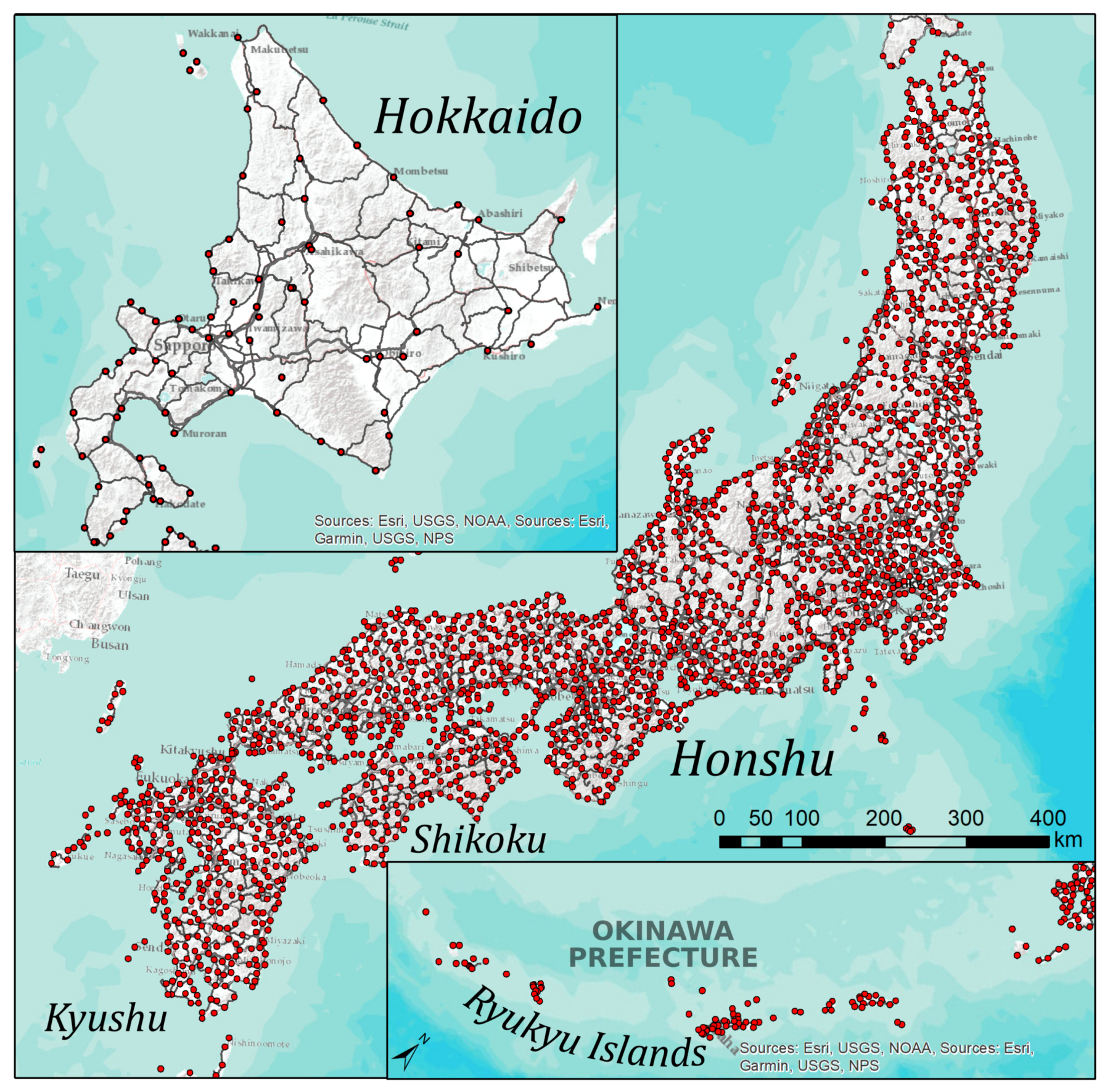
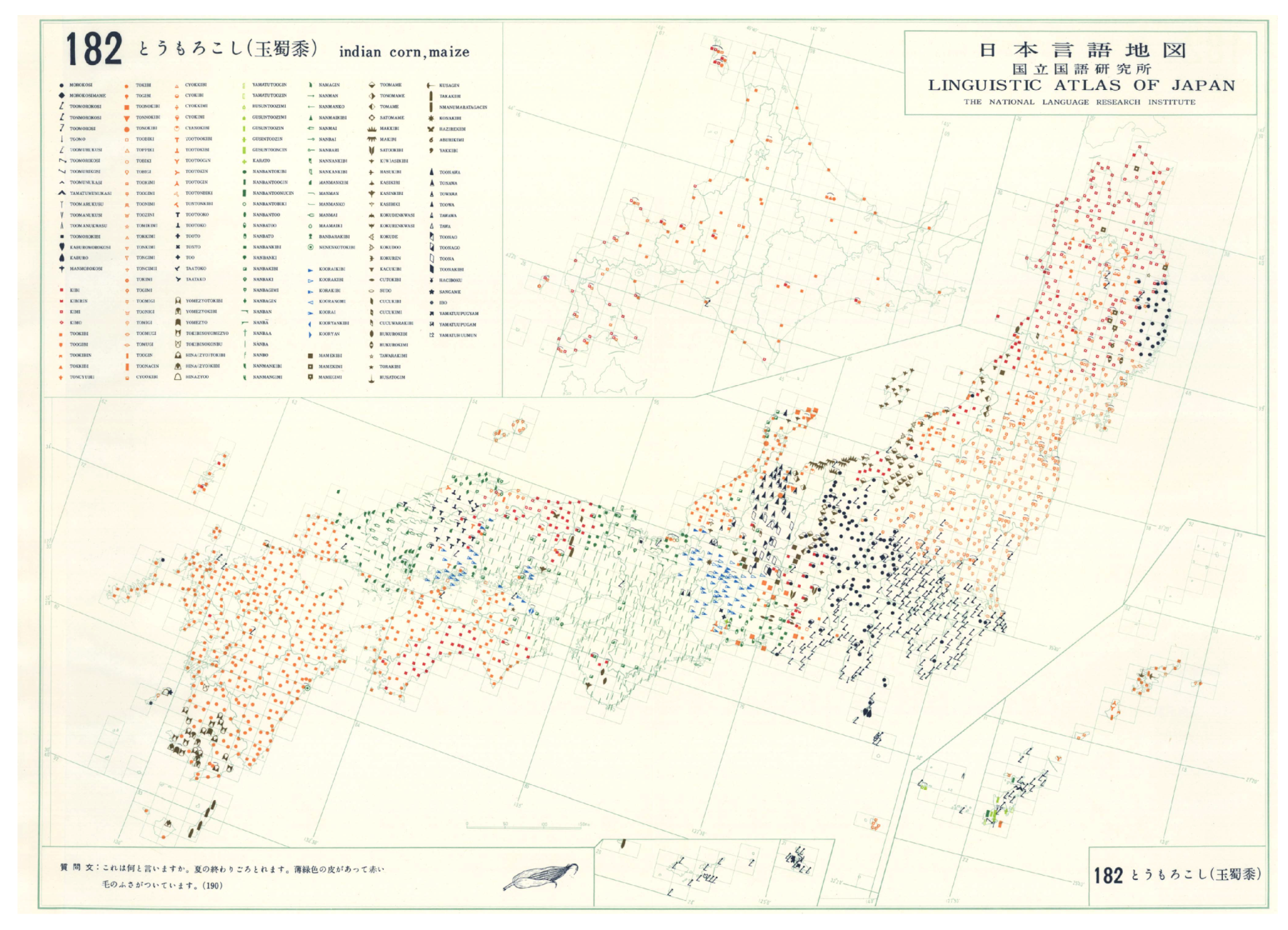
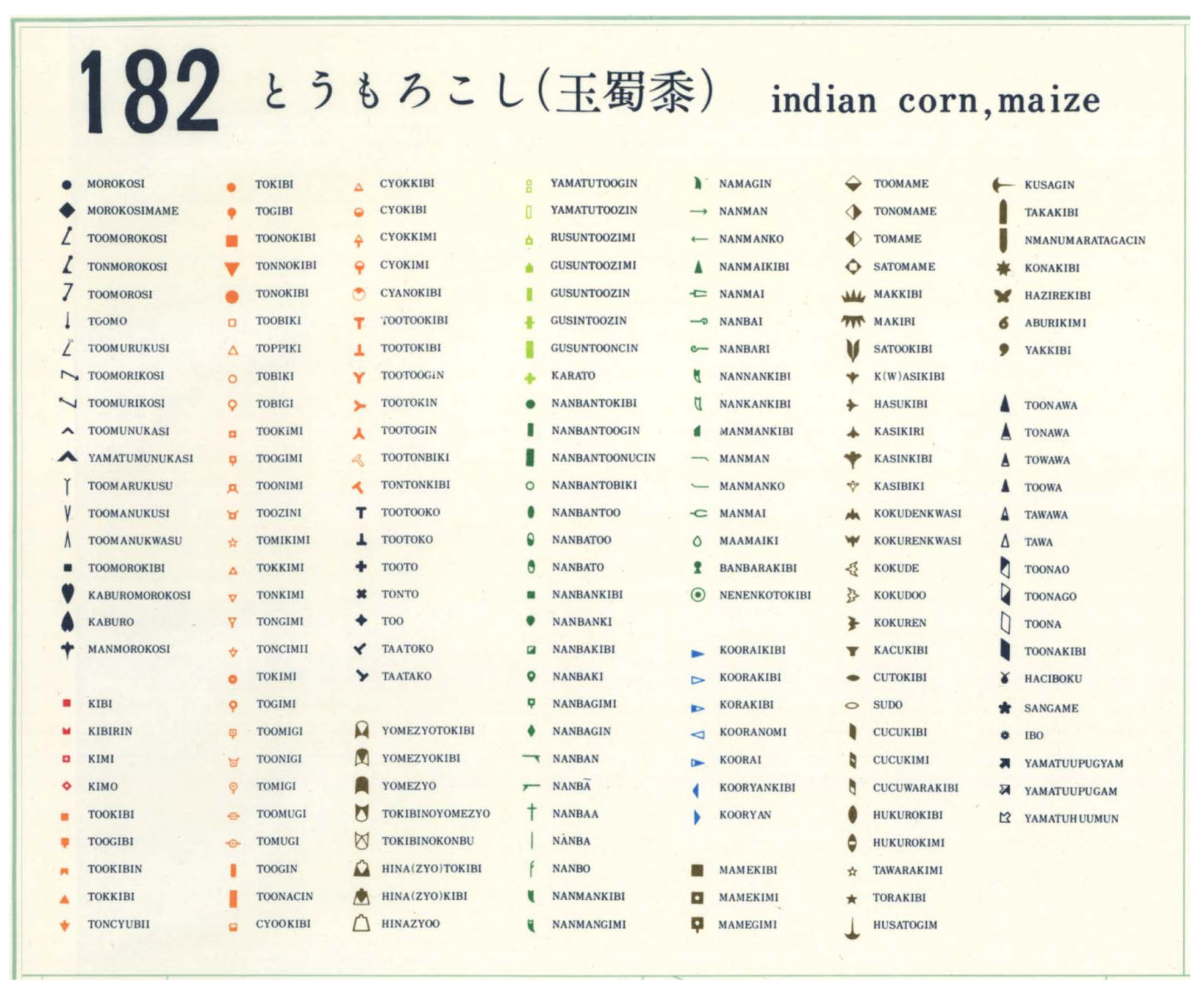
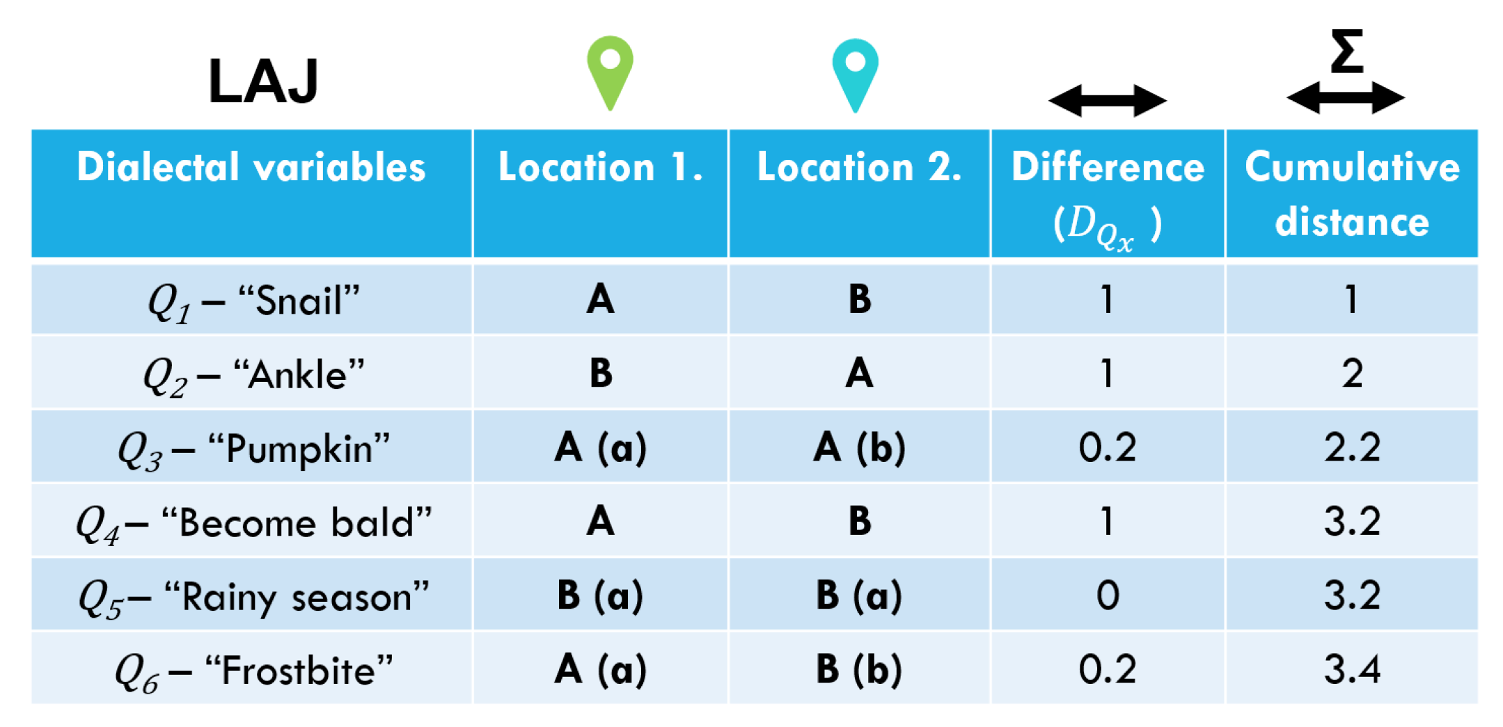
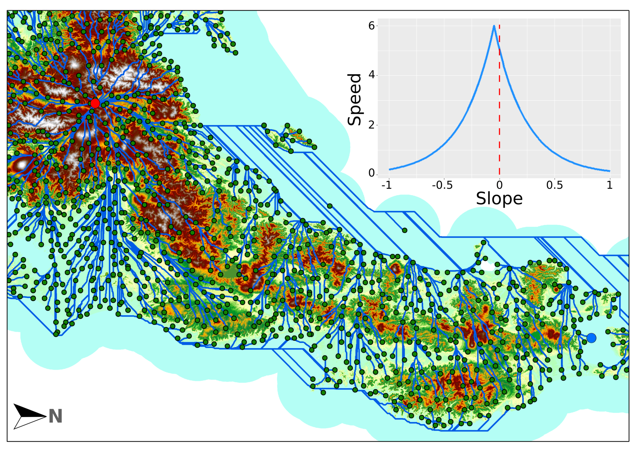
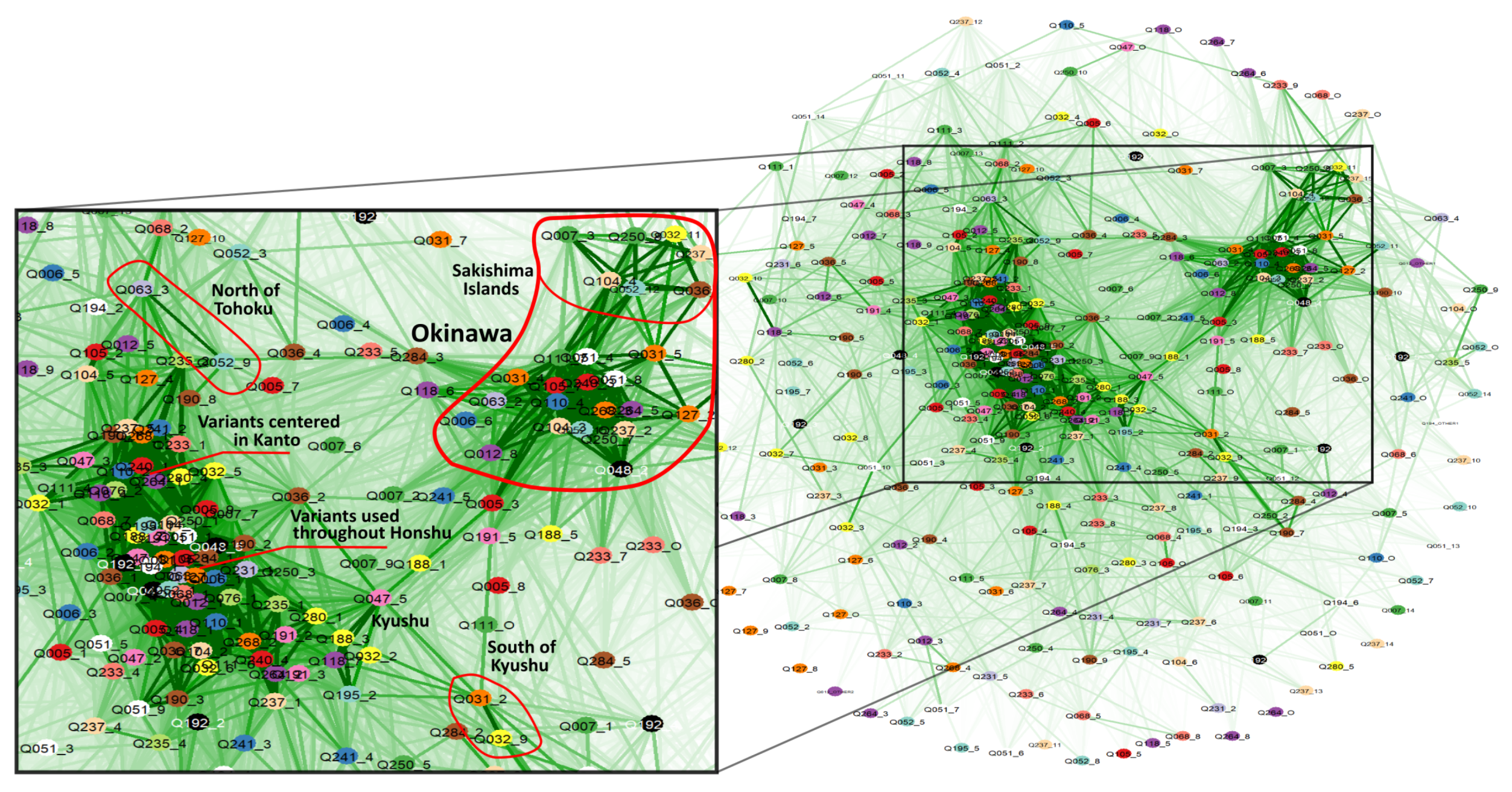
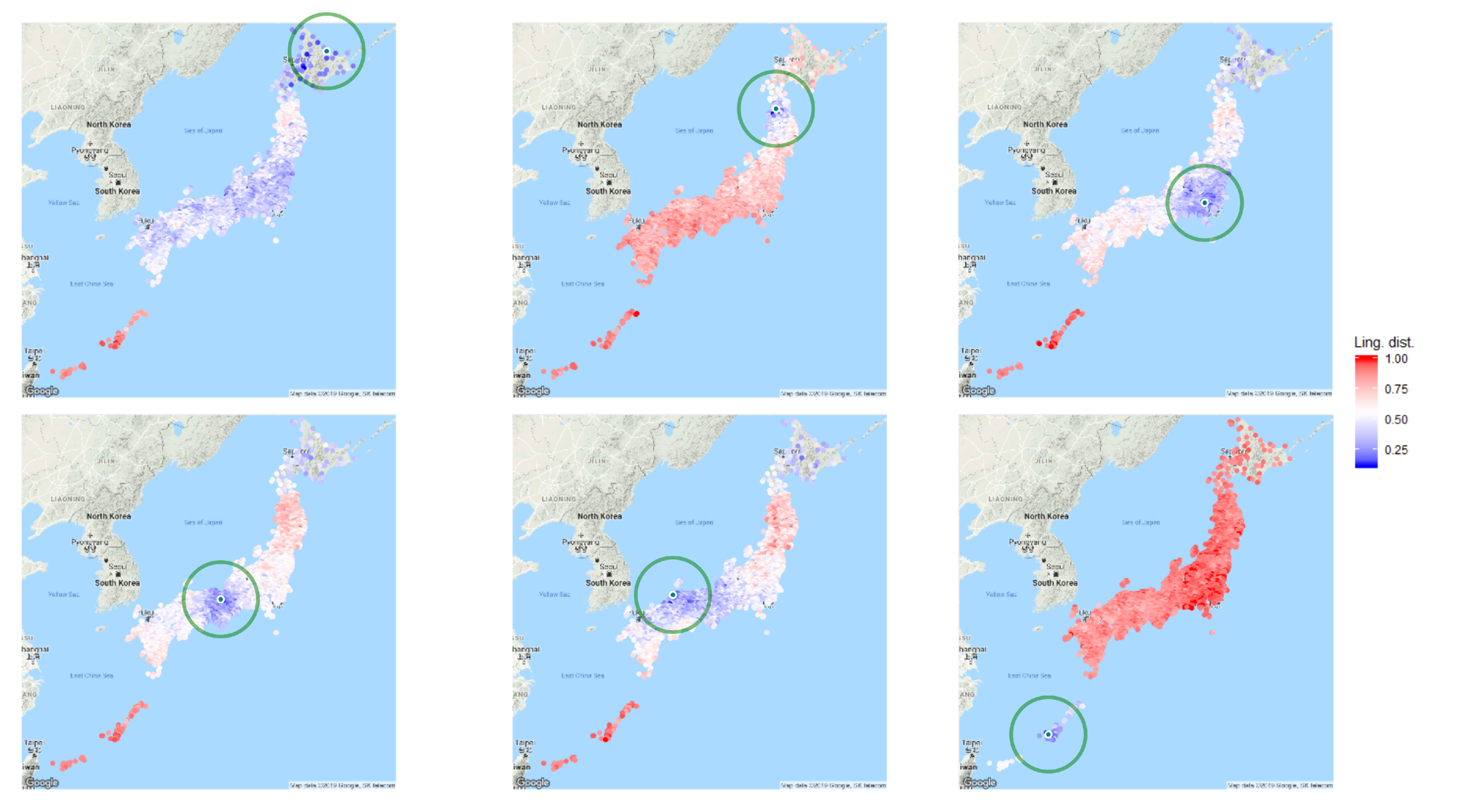
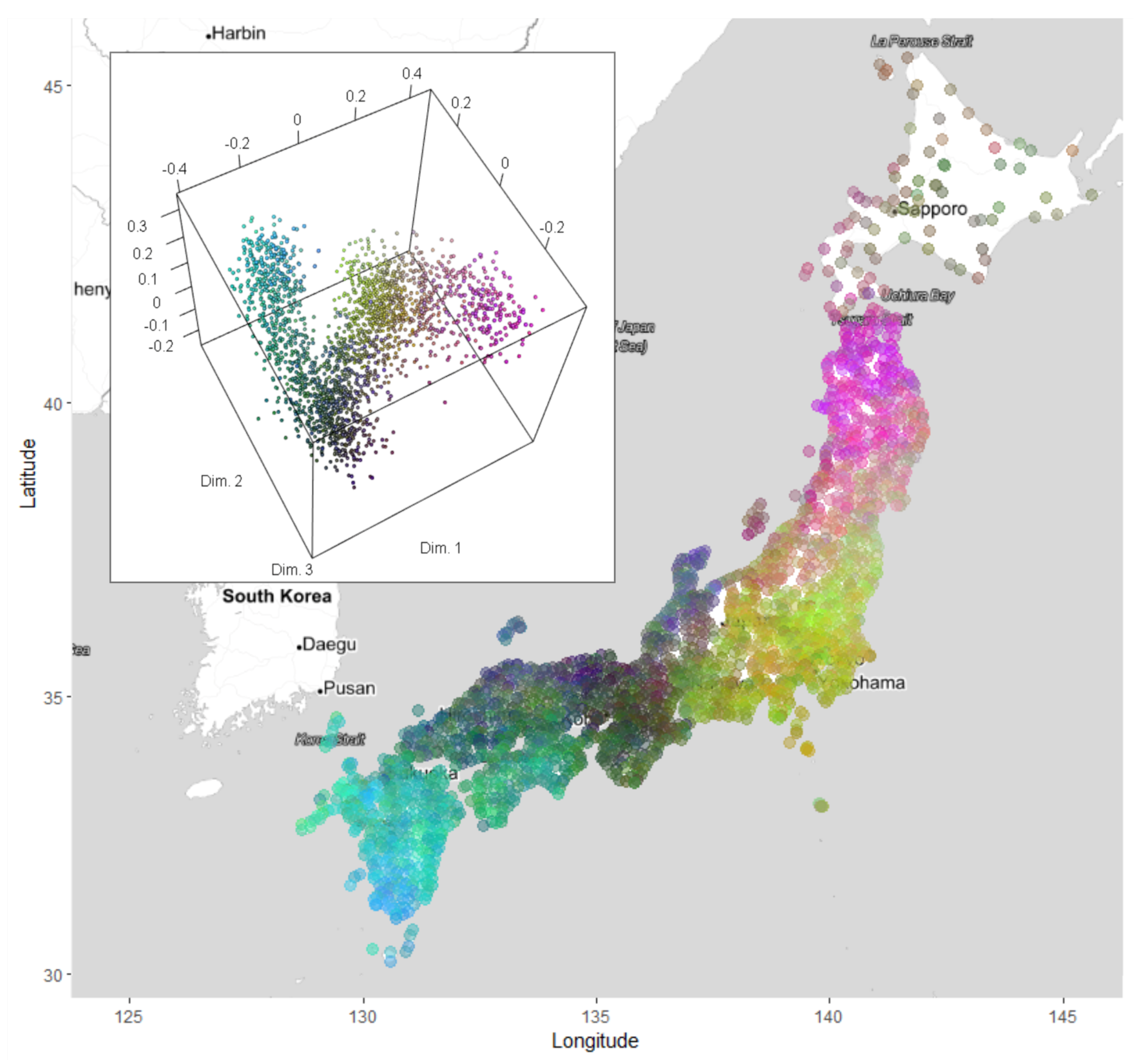
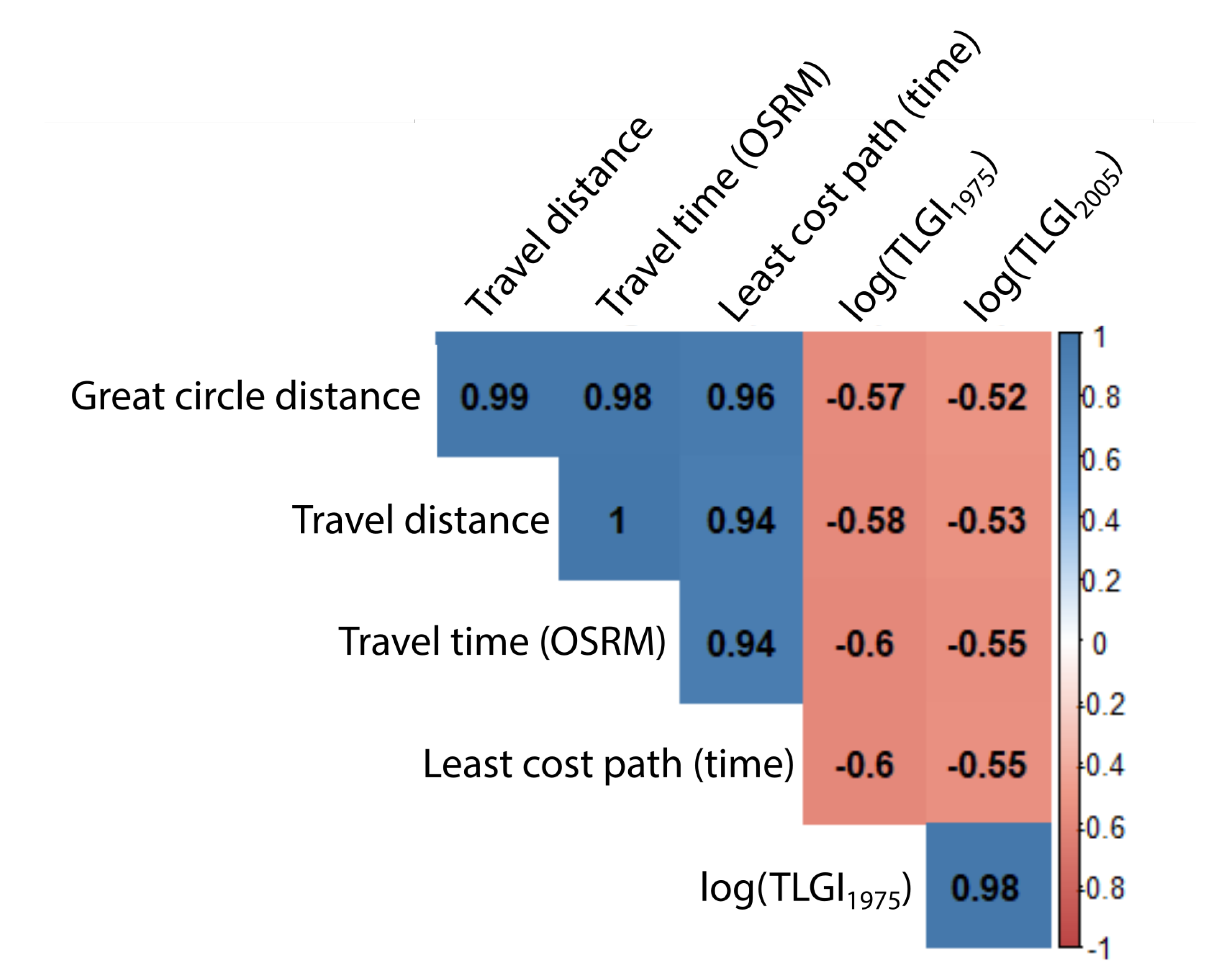
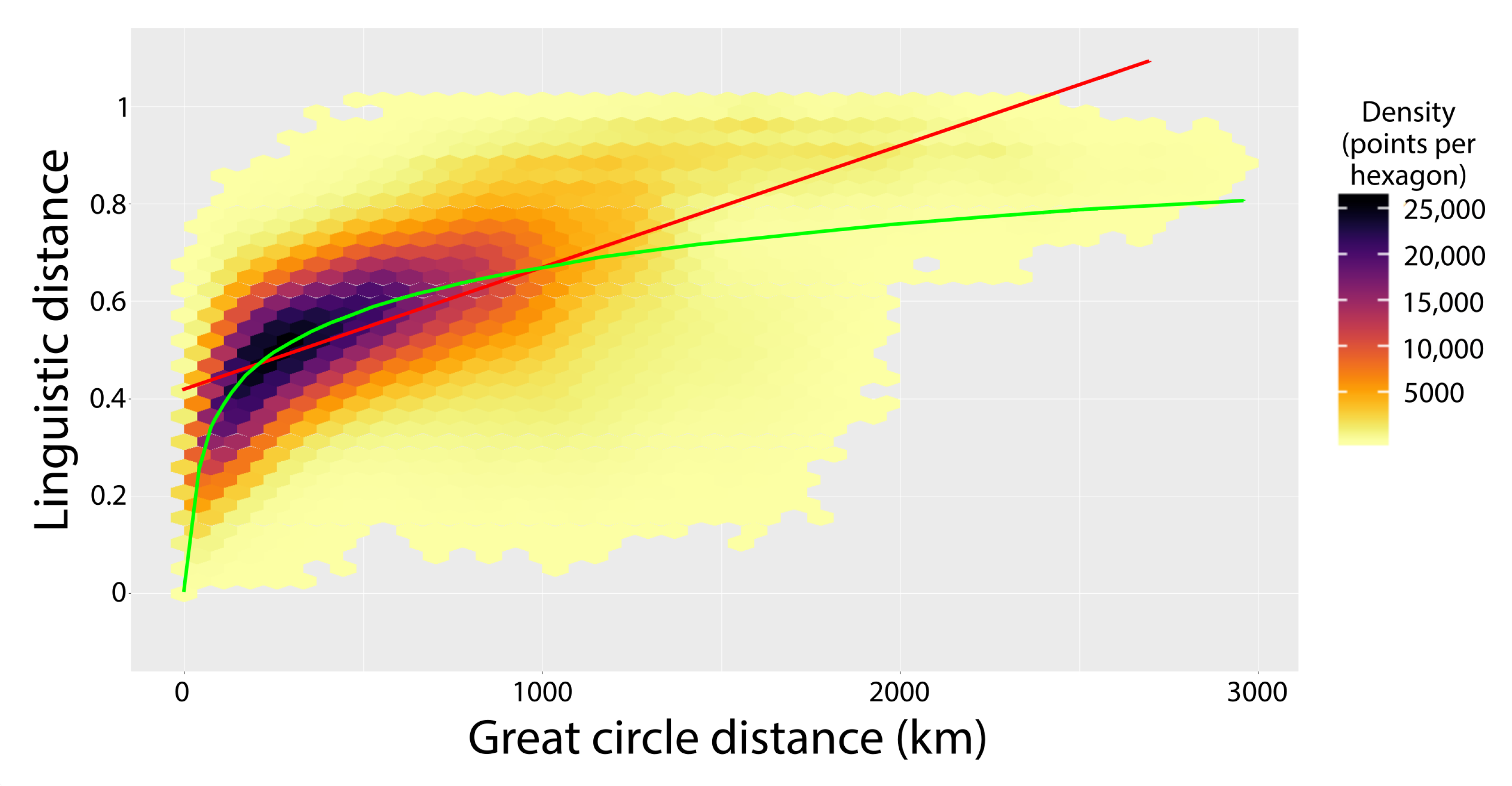
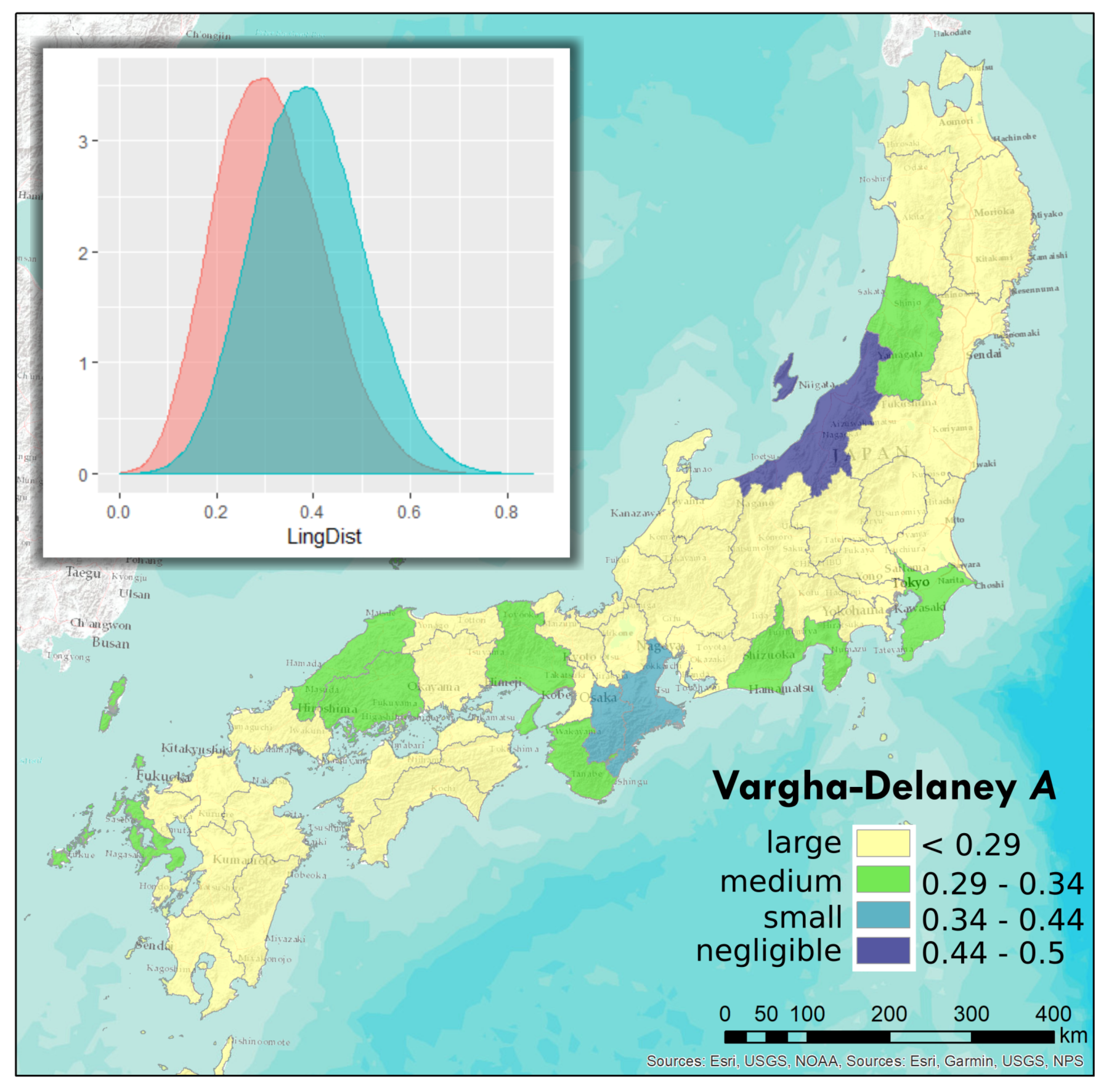
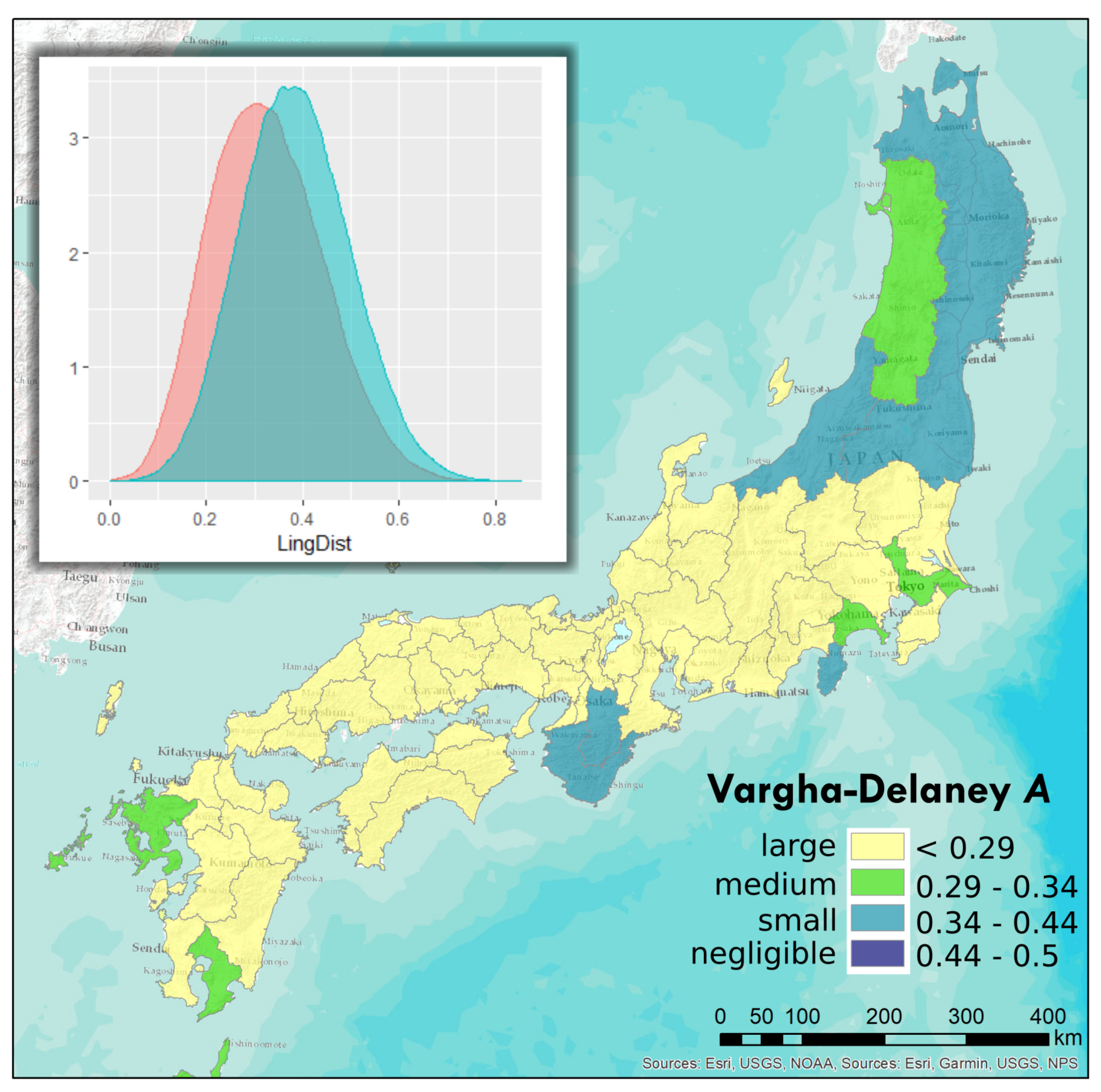
Table 1.
Correlation coefficients expressed as Pearson’s r. For each set the number of localities included are given in parentheses. means the survey location pairs with no missing values, i.e., where all spatial distances can be calculated. HSK stands from the set composed of Honshu, Shikoku and Kyushu. * Travel distance has a missing value proportion of 29.27% while ** Travel times have a missing value proportion of 3.14%, Okinawan location pairs have very few non-missing values for TD and TT.
| Entire Area (2400) | L | Hokkaido (83) | Honshu (1666) | HSK (2125) | Shikoku (141) | Kyushu (318) | Okinawa (82) | |
|---|---|---|---|---|---|---|---|---|
| GCD | 0.6462 | 0.6672 | 0.2487 | 0.6488 | 0.6673 | 0.7391 | 0.7237 | 0.6999 |
| log(GCD) | 0.6714 | 0.7048 | 0.2339 | 0.6876 | 0.7037 | 0.7824 | 0.7544 | 0.7718 |
| TD * | 0.6613 | 0.6613 | 0.2564 | 0.6713 | 0.6606 | 0.7602 | 0.7246 | 0.3902 |
| log(TD) * | 0.7058 | 0.7057 | 0.2441 | 0.7126 | 0.7055 | 0.7943 | 0.7561 | 0.4139 |
| TT ** | 0.5322 | 0.6681 | 0.1773 | 0.5023 | 0.6675 | 0.5456 | 0.5493 | 0.7573 |
| log(TT) ** | 0.6717 | 0.7087 | 0.2782 | 0.6622 | 0.7072 | 0.6923 | 0.7357 | 0.7454 |
| HT | 0.5836 | 0.6718 | 0.2177 | 0.6605 | 0.6719 | 0.7548 | 0.6786 | 0.5739 |
| log(HT) | 0.6078 | 0.6834 | 0.2115 | 0.669 | 0.6845 | 0.7693 | 0.664 | 0.6848 |
| TLGI1975 | −0.5078 | −0.5188 | −0.3539 | −0.4919 | −0.5182 | −0.6454 | −0.5498 | −0.6078 |
| TLGI2005 | −0.4695 | −0.4862 | −0.3407 | −0.4627 | −0.4855 | −0.606 | −0.4966 | −0.584 |
Table 2.
Global results of testing the effect of administrative boundaries. The density plots for 150 km distance cut-off cases are presented in Figure 12 and Figure 13.
| Boundary Type | Distance Cut-off (km) | Vargha-Delaney A | Interpreted Effect Size |
|---|---|---|---|
| Prefectures (47) | 200 | 0.2607 | large |
| Prefectures (47) | 150 | 0.3045 | medium |
| Prefectures (47) | 100 | 0.3473 | small |
| Prefectures (47) | 50 | 0.3793 | small |
| Domains (68) | 200 | 0.5387 | negligible |
| Domains (68) | 150 | 0.3513 | small |
| Domains (68) | 100 | 0.3725 | small |
| Domains (68) | 50 | 0.4079 | small |
© 2019 by the authors. Licensee MDPI, Basel, Switzerland. This article is an open access article distributed under the terms and conditions of the Creative Commons Attribution (CC BY) license (http://creativecommons.org/licenses/by/4.0/).
Share and Cite
MDPI and ACS Style
Jeszenszky, P.; Hikosaka, Y.; Imamura, S.; Yano, K. Japanese Lexical Variation Explained by Spatial Contact Patterns. ISPRS Int. J. Geo-Inf. 2019, 8, 400. https://0-doi-org.brum.beds.ac.uk/10.3390/ijgi8090400
AMA Style
Jeszenszky P, Hikosaka Y, Imamura S, Yano K. Japanese Lexical Variation Explained by Spatial Contact Patterns. ISPRS International Journal of Geo-Information. 2019; 8(9):400. https://0-doi-org.brum.beds.ac.uk/10.3390/ijgi8090400
Chicago/Turabian StyleJeszenszky, Péter, Yoshinobu Hikosaka, Satoshi Imamura, and Keiji Yano. 2019. "Japanese Lexical Variation Explained by Spatial Contact Patterns" ISPRS International Journal of Geo-Information 8, no. 9: 400. https://0-doi-org.brum.beds.ac.uk/10.3390/ijgi8090400
Note that from the first issue of 2016, this journal uses article numbers instead of page numbers. See further details here.