Multistage Cascade Predictor of Structural Elements Movement in the Deformation Analysis of Large Objects Based on Time Series Influencing Factors

Abstract

Hydropower dam displacement is influenced by various factors (dam ageing, reservoir water level, air, water, and concrete temperature), which cause complex nonlinear behaviour that is difficult to predict. Object deformation monitoring is a task of geodetic and civil engineers who use different instruments and methods for measurements. Only geodetic methods have been used for the object movement analysis in this research. Although the whole object is affected by the influencing factors, different parts of the object react differently. Hence, one model cannot describe behaviour of every part of the object precisely. In this research, a localised approach is presented—two individual models are developed for every point strategically placed on the object: one model for the analysis and prediction in the direction of the X axis and the other for the Y axis. Additionally, the prediction of horizontal dam movement is not performed directly from measured values of influencing factors, but from predicted values obtained by machine learning and statistical methods. The results of this research show that it is possible to perform accurate short-term time series dam movement prediction by using machine learning and statistical methods and that the only limiting factor for improving prediction length is accurate weather forecast.

1. Introduction

The dams are very important for production of electric energy, water supply, and irrigation. However, at the same time they pose a great danger for the area situated downstream. To prevent any hazardous influence of the dam, it is important to perform constant monitoring. Lombardi [1] formulated the objectives of dam monitoring by posing four questions:

• Does the dam behave as expected/predicted?
• Does the dam behave as in the past?
• Is there any trend which could impair dam’s safety in the future?
• Was any anomaly detected in the behaviour of the dam?

Although Lombardi specified that these questions are intended for dam monitoring, they could also apply to any other large infrastructural object. Many authors from various professions use different methods and approaches to answer these questions, but they all have the same goal—to get precise and reliable information about the object’s behaviour and health.

The main goal of this research is to develop an approach that can provide accurate assessment of the current state of a dam and better understand the relationship between influencing factors and the dam movement. The secondary goal is to use this knowledge to make accurate short-term time series prediction of dam displacements based on predicted values of influencing factors.

Accurate prediction of object movement would notably increase object safety and the object maintenance would be much easier. Object monitoring has been and remains in the focus of scientific research, while instruments and technologies are changing over the time. Our main focus is on analysing and prediction horizontal dam movement by machine learning and statistical methods. Horizontal dam movement prediction is conducted by applying two approaches:

• Every influencing factor is predicted independently and predicted values are used for short-term dam movement prediction.
• Influencing factors are predicted considering their interconnectedness and then short-term dam movement prediction is performed.

Therefore, this research is a synthesis of two complementary study areas: structural health monitoring (SHM) and time series prediction (TSP). Considerable amounts of research on SHM related to infrastructure objects and natural phenomena (tunnels, bridges, dams, big buildings, landslides, soil and rock masses) has been conducted in recent years. The main focus is on the analysis and prediction of dam movement. Conventional geodetic measurements still play major role in dam stability monitoring. However, recent studies show that researchers are increasingly using Global Navigation Satellite System (GNSS) and remote sensing methods, as the gap in accuracy between these methods and conventional geodetic measurements is steadily decreasing. GNSS and remote sensing methods are now able to achieve accuracy, which satisfies strict demands of dam monitoring.

Yigit, Alcayb and Ceylanb (2015) evaluate the horizontal movements of the Ermenek Dam (Turkey) based on periodic conventional geodetic measurements during the first filling of the reservoir. Dam displacements are correlated to water level in reservoir and seasonal temperature changes. Their analysis reveals that the periodicity and linear trend in the time series are related to seasonal concrete temperature fluctuations increasing linearly with reservoir level. Measured deformations by geodetic methods are in line with the predicted deformation obtained by the Finite Element Method (FEM) analysis [2]. Xiao et al. (2019) investigate performance of GNSS measurements in South-to-North Water Diversion Project in China. GNSS measurements meet temporal and accuracy requirements for deformation monitoring. The study reveals high correlation between the water level in the reservoir and the deformation of the dam surface [3]. Due to a lack of specific models describing the behaviour of earthen dam, Dardanelli and Pipitone (2017) tested several hydraulic models and FEM. To additionally support their research, GNSS measurements over 2 years (2011–2013) are also performed. The best prediction results are obtained by the PoliMi model and the deterministic model (difference between measured and observed data are in a range of a few millimetres). By comparing data obtained by GNSS and traditional geodetic measurements, it is evident that satellite survey has great potential for SHM [4]. Teng et al. (2011) propose permanent scatterer application and quasi permanent scatterer time-series Interferometric Synthetic Aperture Radar (InSAR) images for dam monitoring. The results of their proposed dam monitoring approach, by using time-series SAR images, are in line with those obtained by conventional methods. In conclusion, authors emphasised that the proposed approach does not require field work, as coverage of SAR images allows deformation monitoring on a large scale and due to density of observation number of observed points is much higher compared to conventional methods [5]. SAR images are employed in study at Svartevatn earth-rockfill dam (Norway) by Voege, Frauenfelder and Larsen (2012). By using SAR images dam displacements and mean ground velocity are calculated. Their results show that historic SAR data can be used to monitor deformations of the dam with a resolution comparable to conventional geodetic measurements [6]. Dardanelli et al. (2014) developed continuous GNSS system for earth-dam deformations monitoring in Sicily (Italy). Their research reveals that accuracy of post-processed GNSS measurements is comparable to conventional geodetic methods. Also, correlation between changes of reservoir surface, obtained by remote sensing methods, with obtained GNSS displacements was calculated in this study and results showed weak positive correlation between tested variables [7]. Levelling, GPS measurements and SAR images are used to evaluate stability of the Darbandikhan dam (Iraq) after high magnitude earthquake in research conducted by Al-Husseinawi et al. (2018). Their research concludes that SAR images of the post-seismic dam deformation are useful to inform maintenance plans, but terrestrial surveys are still essential in the case of large-gradient deformation during earthquakes [8].

Although, conventional dam deformation methods have very high accuracy, they are time consuming, labour intensive, and have high costs. On the other hand, GNSS measurements offer continuous monitoring of the dam, while remote sensing methods allow deformation monitoring on a large scale and higher density of observation points compared to conventional methods and GNSS. To take advantage of all of these methods, experts usually use integrated approach to obtain best possible monitoring results.

Statistical methods are traditionally used for dam stability analysis and prediction. Application of machine learning methods is also one of the common approaches in SHM. Among machine learning methods, the application of artificial neural networks (ANNs) has the leading role in dam deformation analysis and dam movement prediction. ANNs and statistical methods are used independently or jointly—either to complement each other or for comparison purposes.

Bui et al. (2016) propose application of swarm optimised neural fuzzy inference system (SONFIS) for modelling and forecasting of the horizontal displacement of hydropower dams. Time series monitoring data (horizontal displacement, air temperature, upstream reservoir water level and dam aging) of the Hoa Binh hydropower dam (Vietnam) are selected as a case study. SONFIS model outperforms support vector regression, multilayer perceptron neural networks, Gaussian processes, and Random forests that use the same data for model fitting and testing [9]. In the same case study, the multi regression model (MLR), SARIMA model and the back-propagation neural network (BPNN) merging models are tested for dam movement prediction by Zou et al. (2017). Authors conclude that SARIMA model and the SARIMA–BPNN merging model have great potential applications in the field of dam deformation analysis and prediction [10]. Liu et al. (2018) developed a self-diagnosis system for dam safety diagnosis. Their system is based on the gray model-genetic algorithm-BPNN model and can realise online fault diagnosis better than the traditional single models [11]. Application of an extreme learning machine (ELM), feedforward neural network with a single layer of hidden nodes with the weights connecting inputs to hidden nodes are randomly assigned, is proposed for displacement prediction of gravity dams by Kang et al. (2017). Proposed model is compared to BPNN, MLR and stepwise regression models and the results show that proposed model has better accuracy and requires less time for model fitting [12].

Time series prediction (TSP) provides a wide span of applications in engineering, energy production and management, tourism and stock exchange. Similarly to SHM, statistical methods and machine learning methods are commonly used in TSP. Autoregressive integrated moving average (ARIMA) with or without seasonal component (SARIMA) is very popular among researchers. Due to climate changes, there are numerous studies dealing with meteorological and hydrological prediction and one of the most popular methods is ARIMA. It is rather common to use different types of ANNs for TSP, especially recurrent dynamic networks with feedback connections such as: nonlinear autoregressive neural networks (NAR) and nonlinear autoregressive neural networks with exogenous inputs (NARX).

In research conducted by Murat et al. (2018), meteorological time series data from different climatic zones are used for fitting Box-Jenkins and Holt-Winters SARIMA, ARIMA with external regressors in the form of Fourier terms and the time series regression. The results show that chosen models cannot predict the exact air temperature and precipitation but they can give information that helps environmental planning and decision-making [13]. Chawsheen and Broom (2017) use SARIMA model for monthly mean temperature prediction in Erbil (IRAQ). The selected model is validated by predicting the mean temperature from January 2014 to November 2015 and the estimated forecast mean temperature is identical or very close to the actual temperature data. Authors conclude that proposed model could be also applied to accurately determine the need for electricity and water in the Kurdistan Region of Iraq [14]. In research conducted by Rizkina, Adytia and Subasita (2019), NAR networks and tidal harmonic analysis are used for sea level prediction in Semarang (India). NAR networks show better results compared to tide harmonic analysis, which is standard method for seal level prediction [15]. Cadenas et al. (2016) compare performance of univariate ARIMA and multivariate NARX model for short term wind speed prediction. The results show that multivariate NARX model gives more accurate results when compared to ARIMA model. Although, NARX model outperformed ARIMA model, authors point out that even univariate ARIMA model can give reasonable one step ahead wind speed prediction [16]. Hamzic et al. (2016) compared NAR networks and Feed Forward Back Propagation neural networks for short-term water level prediction in reservoir. The results showed that neural networks can provide quality water level prediction even if only water level data is used. The main weakness of univariate time series water level prediction is slow adjustment to sudden water level changes. [17].

Unlike standard daily surveying measurements, which can be performed by using standard geodetic equipment, dam monitoring demands very precise instruments and special conditions should be met to achieve the required accuracy and reliability of measurements. To obtain desired results it is necessary to [18,19,20]:

• Establish special control geodetic network whose accuracy is better than standard geodetic networks (e.g., state geodetic network). These control networks are used for displacement and deformation measurements. However, it is not enough just to determine the existence of displacements. It is also necessary to determine how reliable these measurements are. Special geodetic networks cover not only complete deformation area but also area where no deformations are expected (stable ground). Moreover, network shape should be carefully determined because only geometrically stable and reliable network enables high accuracy and reliability needed for deformation analysis.
• Use the best available instruments and measuring techniques. Instruments and other equipment are regularly inspected and rectified in authorised institutions to confirm their operational correctness. Modern instruments used for deformation monitoring are not only very precise and fast but also designed in such a way that occurrence of any type of error is minimised (automatic aiming and saving measurements directly in programs for data processing).
• Repeat every measurement in order to ensure reliability of results. Angle measurements are performed in two faces of total station to reduce systematic errors and distances are measured with every angle measurement.
• Measure atmospheric parameters (air temperature, air pressure and humidity) and use them later for measurement corrections. Earth shape and refraction is also considered when preparing data for processing.

Even with all precautions taken and above procedures followed, some errors do occur in measurements. These errors are removed with special statistic tests and only valid measurements are used for deformation analysis.

Dam monitoring by using precise geodetic surveying is very accurate but also time-consuming method for dam stability analysis. It gives global picture of the object’s health and is very highly regarded among the professionals. This method requires group of experts, using special instruments and methods. Hence it is usually performed only twice a year. The first annual monitoring series is conducted when the dam accumulates all the cold, which is at the end of winter and early spring, and second annual monitoring series is conducted when the dam accumulates all the heat which is at the end of summer and early autumn.

The main issue with modelling current state of the dam and dam movement prediction is general lack of dam monitoring data obtained by precise geodetic surveying and unfavourable data distribution—all measurements are performed at approximately the same time of the season and under similar conditions. Accordingly, there are no satisfactory quantities of dam monitoring data by precise surveying which may be used for detailed analysis and research. Although it is possible to automatise this process, it is very rarely implemented in practice due to high costs of needed instruments and equipment. Often less accurate methods are used for dam monitoring especially if they can be easily automated or performed quickly.

To overcome these above mentioned issues for the purpose of this research a total of 20 series of distance and angular measurements by precise robotic total station is conducted in period from 15 January 2015 to 7 April 2017 (approximately one measurement every 41 days). Of 20 measurement series, 18 were used for model fitting and two were used for external validation.

All geodetic measurements were carried out by using precise robotic total station in combination with Terrestrial Positioning System Control software and GNSS/LPS/LS based Online Control and Alarm System (GOCA) software was used for measurement processing [21,22]. All temperature measurements, water inflow/outflow and water level measurements are preprocessed and visualised by MS Excel. ANN training and ARIMA model fitting and prediction has been performed by MATLAB 2018. Time series data of influencing factors and measured dam displacements of the Jablanica hydropower dam were selected as a case study.

Even all data regarding dam monitoring were collected by carefully following regulations and procedures, some false readings and missing data still appear. Thus, the first step was “cleaning” the data from false readings and supplementing the missing data. The second step was to find optimal ANNs structures and ARIMA models for short-term prediction of influencing factors. In the third step, correlation between dam movements and influencing factors is determined by using localised approach—individual models are developed for every point strategically placed on the object. The final step was to perform short-term dam movement prediction by using predicted values of influencing factors. Predicted values are compared to the observed displacement to validate the proposed model.

The results prove it is possible to perform very accurate short-term dam movement prediction by using predicted values of influencing factors. Although, dam movement is complex and nonlinear, the results show that there is a strong linear correlation between influencing factors and dam movement in the direction of river flow for all object points distanced from dam foundations.

2. Materials and Methods

2.1. The Case Study

The dam in Jablanica is an arch-gravity concrete dam 85 m high with the crest length of 210 m. It was built on the river Neretva in 1955 approximately five kilometres north from the centre of Jablanica (Bosnia and Herzegovina). After the construction, it was the largest waterpower object in the former Socialist Federal Republic of Yugoslavia [23]. A network for physical and geodetic monitoring is installed on the dam in order to inspect a current state of dam’s health. The dam is equipped with sensors that measure: air temperature, water temperature, concrete temperature, displacements between dam blocks, dam blocks inclination, uplift water pressure and pressure of underground water. These sensors collect data in the form of time series.

Time series data is any data that is observed sequentially over time. The goal of time series prediction is to estimate future values based on present and historical data, or stated mathematically [24]:

$$\tilde{\mathrm{y}}(\mathrm{t}+\mathsf{\Delta }\mathrm{t})=\mathrm{f}\left(\mathrm{y}\right(\mathrm{t}-1), \mathrm{y}(\mathrm{t}-2), \mathrm{y}(\mathrm{t}-3),\dots ,\mathrm{y}(\mathrm{t}-\mathrm{n}\left)\right),$$

(1)

where $\tilde{\mathrm{y}}$ is the predicted value of a time series y, t is the current moment in time, $\mathsf{\Delta }\mathrm{t}$ defines how far in future is predicted and n is the total number of samples.

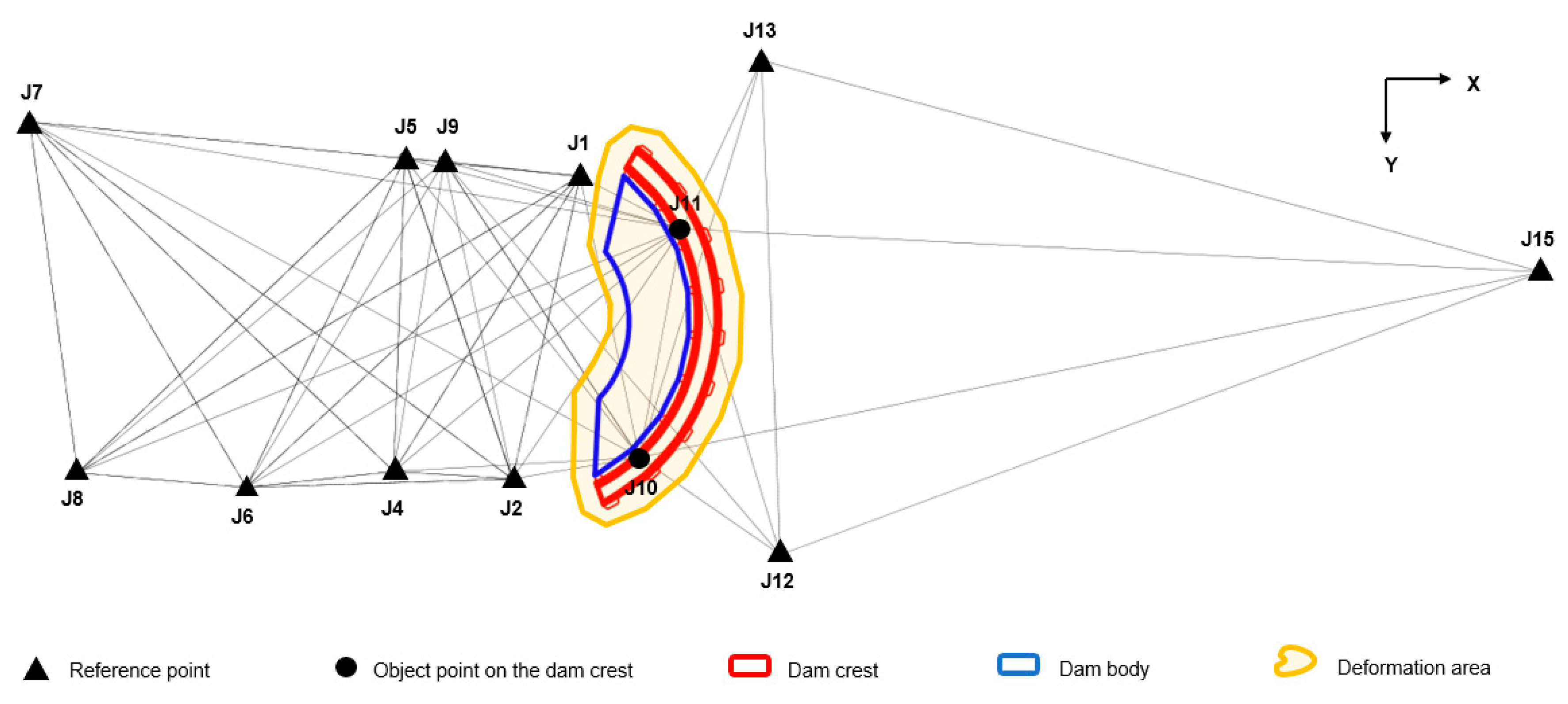
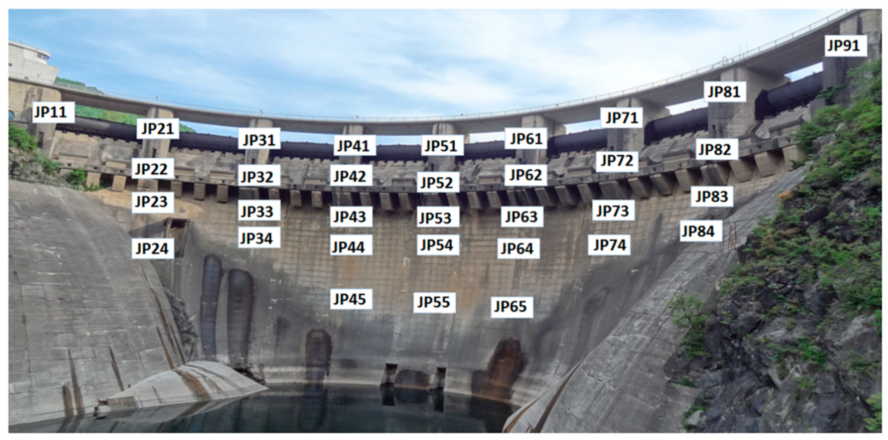
A geodetic network consisting of 11 reference points was used as a base for geodetic monitoring of the dam displacements and 34 object points were monitored. Two object points, geodetic pillars J10 and J11, are installed on top of the dam crest, while the remaining 32 points are installed on the downstream side of the dam body. The main function of points J10 and J11 is not dam deformation monitoring but to improve connection between upstream and downstream reference points, i.e., to enhance the quality of control geodetic network for dam monitoring. Object point JP84 is incorrectly installed and cannot be observed from any reference point, hence it is not included in the research. Reference points network and object points network used for dam monitoring are shown in Figure 1 and Figure 2.

Each geodetic pillar has special stainless steel plate installed on top of it, so a tribrach is directly fastened on the pillar. Hence, there is no instrumental centring error. Horizontal directions, zenith angles and distances are observed from each reference point toward all reference and object points that can be observed. Three sets of observations in two faces are performed from each reference point and atmospheric data are recorded for every set of measurements so measurement corrections can be applied in the post processing. Air temperature and pressure are measured on site while data regarding air humidity is taken from the web weather services.

All observations are performed by precise robotic total station Sokkia NET05 (0.8 mm + 1 ppm distance measurement accuracy, 0.5″ angle measurement accuracy). Leica GPR121 professional prism was used for observations on geodetic pillars and Sokkia Mini102 prisms with custom made holders are installed on the dam body.

Coordinate system for the dam monitoring is defined as follows:

• X axis passes through the geometric centre of the dam and the positive direction of X axis is upstream,
• Y axis is perpendicular on X axis and positive direction is towards left coast of the river Neretva,
• H axis-height.

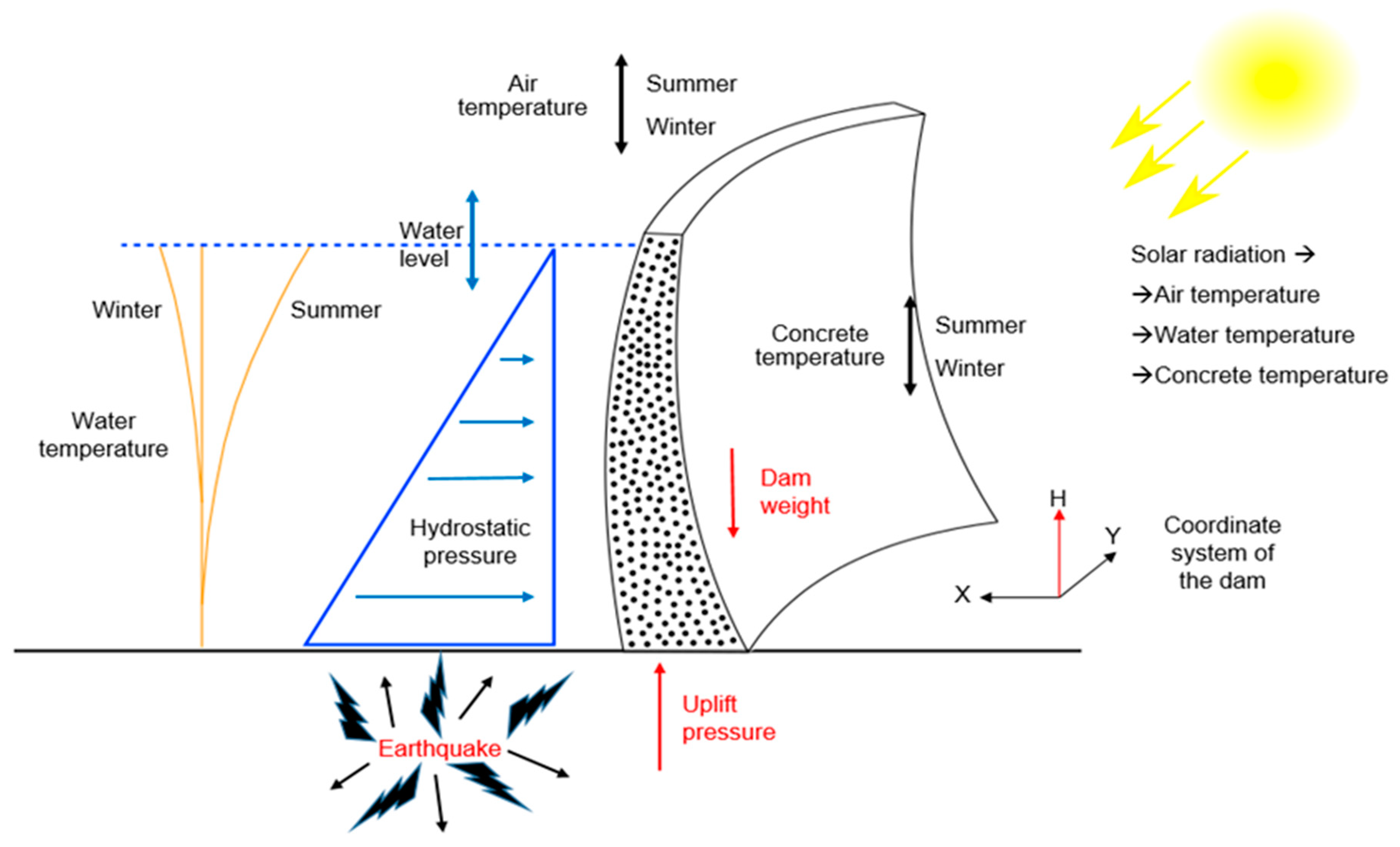
Dam movement is influenced by various factors and the most common factors are presented in Figure 3. Factors which are difficult to model (e.g., earthquakes), factors with insignificant influence (e.g., ice pressure) and factors that do not influence horizontal dam movements (dam weight, uplift pressure) are not considered. The main focus in this research is on four factors that are the main cause for horizontal dam movement: water level, air temperature, water temperature and concrete temperature. Dam ageing is not considered as an important factor since dam movement prediction is performed for a very short time period and the value of this impact factor would be insignificant in this particular case.

2.2. Dam Displacement Data

Dam monitoring with the use of geodetic methods started in 1954 (the initial monitoring series also known as “0” monitoring series) and is usually performed only twice a year. The main problem with geodetic measurements from 1954 to 2015 is that all measurements were performed with no regard to influencing factors, i.e., during these measurements, values of influencing factors were not measured simultaneously to geodetic measurements. Since 2012, the dam monitoring has been performed with the use of precise geodetic surveying by robotic total station and every measurement is accompanied by the appropriate atmospheric data (air temperature, humidity and air pressure) so every measurement can be corrected in accordance with these factors. Automatization of geodetic measurements improved speed of data collecting and also eliminated the majority of human errors from measurements (e.g., wrong data entry or reflector aiming error). Corrected measurements are processed by using GOCA software.

GOCA is a multi-sensor system which applies GNSS/GPS, terrestrial sensors (e.g., total stations, spirit levelling and hydrostatic levelling instruments) and local sensors for deformation monitoring and analysis. As a result, GOCA provides displacements, velocities, and accelerations in a three-dimensional coordinate system [21].

A certain number of measurements needs to be known in order to solve a mathematical model (to obtain coordinates of stable and object points). If more than necessary measurements are added for a solution (redundancy), a discrepancy in the model will occur. To eliminate these discrepancies it is necessary to adjust the mathematical model. Gauss and Legendre (1806) introduced least squares method to remove discrepancies as follows:

$${\mathrm{v}}^{\mathrm{T}}\mathrm{Pv}=\min ,$$

(2)

where $\mathrm{v}$ is n-dimensional residual vector (${\mathrm{v}}^{\mathrm{T}}$ is transposed residual vector) and $\mathrm{P}$ is weight matrix proportional to inverse variance-covariance matrix of measured variables. This method is used in geodesy to connect measurements and unknown parameters and can be stated by the following equation:

$$\mathrm{f}(\hat{\mathrm{x}},\hat{\mathrm{l}})=0,$$

(3)

where $\hat{\mathrm{x}}$ is n-dimensional vector of adjusted parameters, $\hat{\mathrm{l}}$ is n-dimensional vector of adjusted measurements and zero value on the right side of the equation indicates that there is no more discrepancies in the model.

After the adjustment of measurements, Gauss-Markov model is usually used for geodetic data analysis. This model represents a combination of deterministic and corresponding stochastic model:

$${\mathrm{l}+\mathsf{\epsilon }=\mathrm{Ax}}_{\mathrm{T}},\mathrm{and}$$

(4)

$$\mathrm{E}\left({\mathsf{\epsilon }\mathsf{\epsilon }}^{\mathrm{T}}\right){=\mathsf{\sigma }}_0^2{\mathrm{Q}}_{\mathrm{l}},$$

(5)

where l is n dimensional vector of measurements, $\mathsf{\epsilon }$ is vector of real errors, $\mathrm{A}$ is the first design matrix ($\mathrm{A}=\frac{\partial \mathrm{f}}{\partial \mathrm{x}}$), ${\mathrm{x}}_{\mathrm{T}}$ is vector of real values of unknown parameters, E is expected value, ${\sigma }_0^2$ is variance factor and ${\mathrm{Q}}_{\mathrm{l}}$ is cofactor matrix (${\mathrm{Q}}_{\mathrm{l}}{=\mathrm{P}}^{-1}$). For non-linear dependencies, vector l includes differences between observed and computed values of measurements and ${\mathrm{x}}_{\mathrm{T}}$ includes the improvements of parameter values with respect to a priori values of parameters.

Deformation analysis by GOCA consists of three steps [22]:

• Initialisation—free network adjustment in order to remove errors from measurements using Baarda’s iterative data snooping procedure. Only one error can be removed in every iteration and this process is repeated until all the errors from measurements are removed.
• Network adjustment based on refined measurements. Geodetic reference frame consisting of stable geodetic points, is defined in this step and then final adjustment is performed to determine object points coordinates.
• Deformation analysis—reference points stability testing and object points movement testing.

The data obtained by precise tachymetry measurements have very high accuracy and mean point error of object points never exceeds 0.5 millimetres. It is important to note, that all measurements are performed quickly so values of influencing factors cannot change significantly from the beginning to the end of measurements.

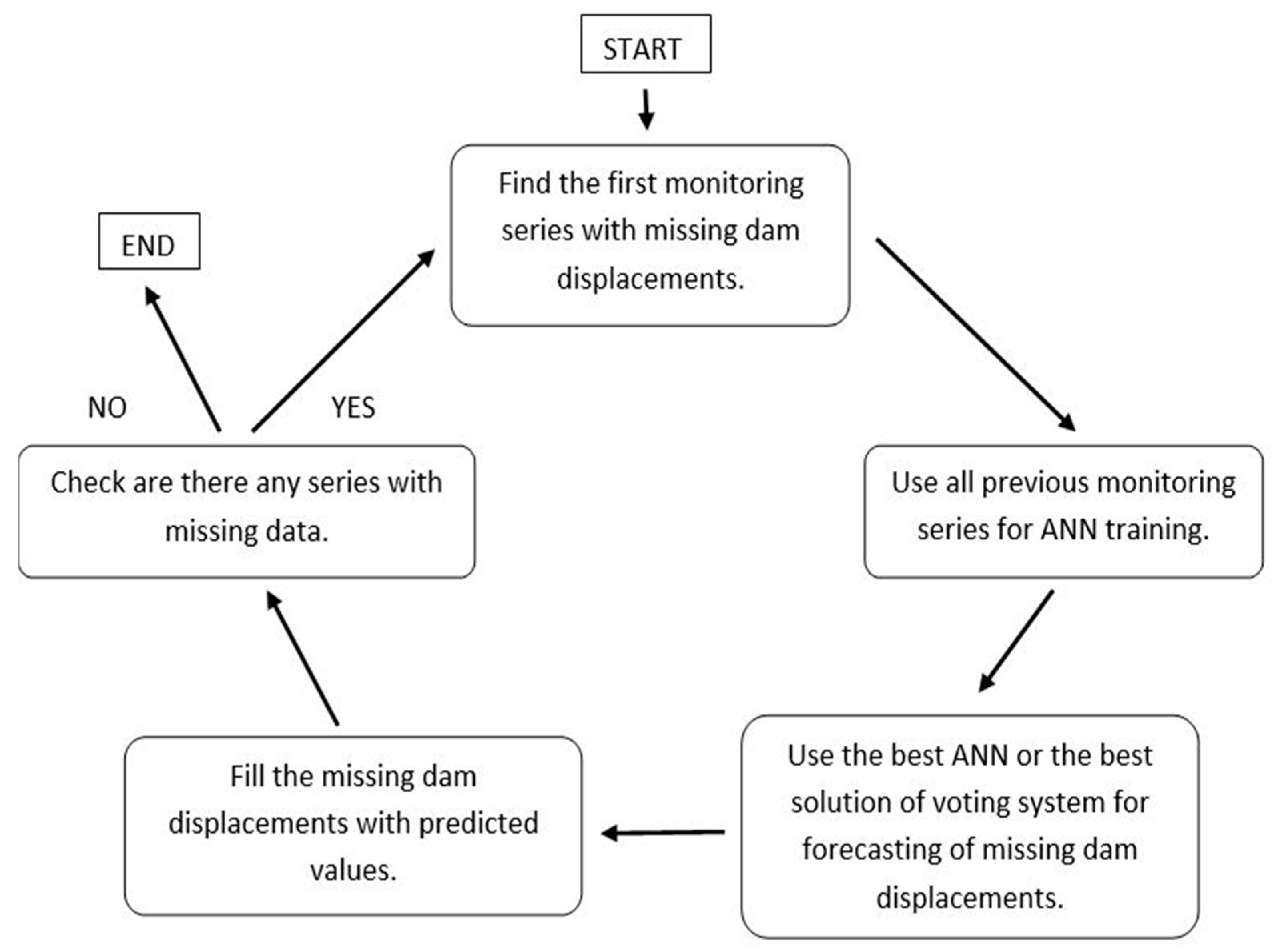
It is often the case that some object points cannot be monitored due to different obstacles (grown tree branch, heavy traffic) or equipment limitations (strong illumination, dirt on the monitoring prisms, tilting terrain). In that case, dam displacements cannot be calculated based on direct observations, but can be interpolated using ANNs prediction [25]. In this research, dam displacements for object point JP24 were interpolated using ANNs prediction for 3 series with missing data (0.48% dam displacement data).

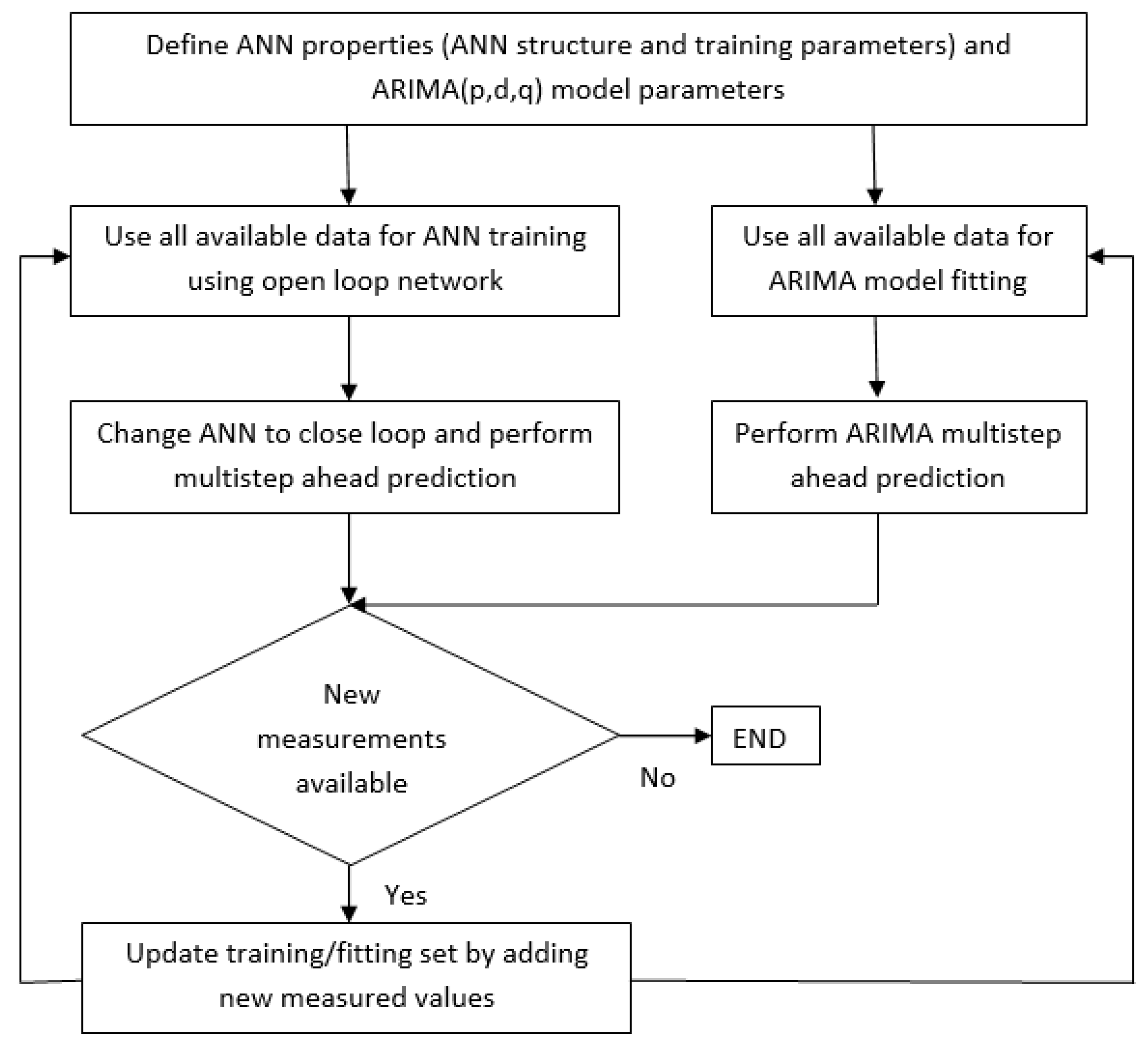
Three types of ANNs (Cascade forward backpropagation, Feed forward backpropagation and Layer recurrent backpropagation) and a voting system with four functions (MIN, MAX, “Mean of closest 2” and “Mean of 3”) were used for the interpolation of missing dam displacements using prediction. Flow chart of proposed model is shown in Figure 4.

The missing data interpolation approach combines spatial and temporal aspects of the data and uses it for its benefits to achieve good results using ANN prediction. It also provides the best results in cases when missing data have a long monitoring history and in cases when there are many neighbouring points near the point with the missing data. Another benefit of this approach is that it can handle missing data at the end of the data intervals. However, the shortcomings of this approach become apparent when a combination of small number of monitoring series and small number of neighbours of the missing object points appears [25].

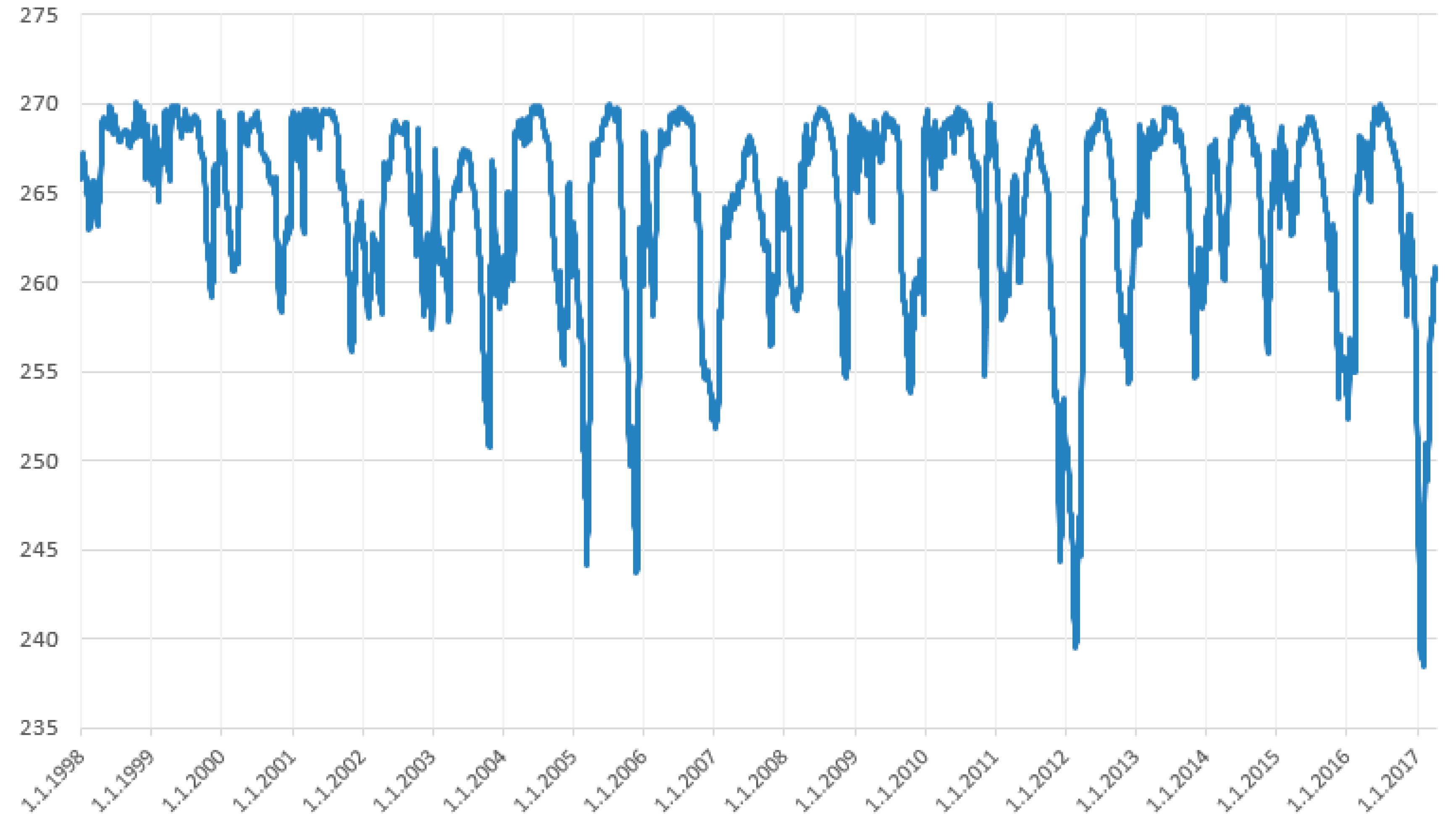
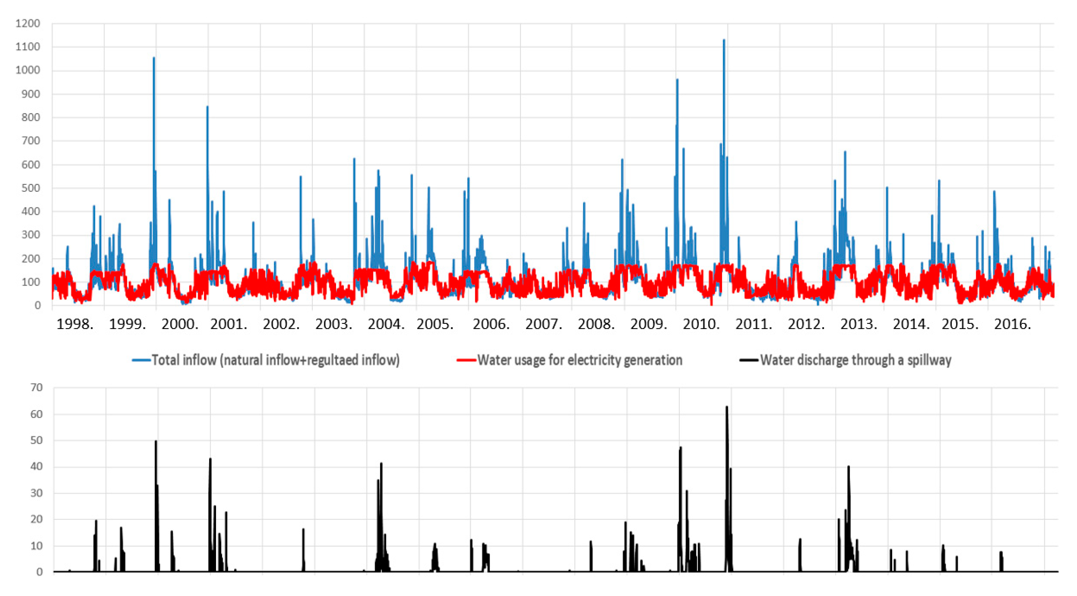
2.3. Water Level Data

Water level in the reservoir is influenced by various factors, such as: inflow, upstream rainfall, discharge of water from reservoir, evaporation and water seepage. We used daily measurements of water level, water inflow, water consumption for the production of electric energy and water discharge over the spillway from 1 January 1998 to 7 April 2017 for ARIMA and ANNs prediction. Since ANNs work better with smaller values, all measured water level values were normalised to values between 0 and 1 for the purpose of ANN training. Collected data is visualised by line graph, shown in Figure 5 and Figure 6, to investigate trends and patterns in water behaviour.

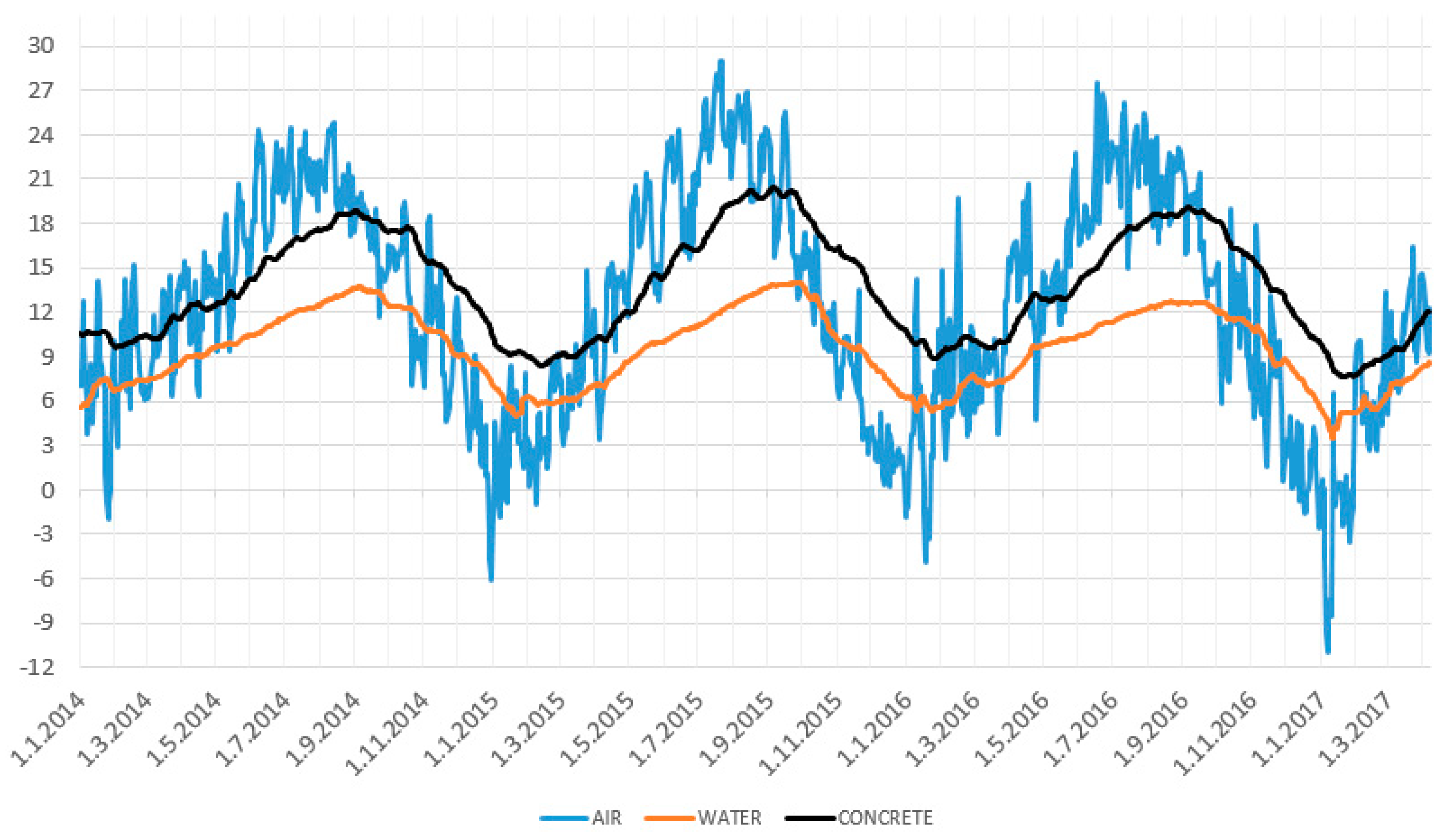
2.4. Air, Water and Concrete Temperature Data

Air, water and concrete temperature data is collected by sensors positioned on the dam and inside of the dam’s structure. Air temperature is measured by one automatic thermometer and one manual mercury thermometer. Water temperature is measured automatically in three vertical levels: 227 m, 240 m and 250 m above sea level (top of the dam’s crest is at 275 m and maximal water level is at 270 m). Measurements were excluded from research in cases when water level was below sensor level. Concrete temperature is measured by numerous sensors evenly distributed inside of the dam’s concrete walls. Values of 9 concrete thermometers positioned on the downstream side of the dam, where geodetic object points are installed, were used. The other sensors are installed inside dam’s galleries walls and their values are almost constant hence these measurements were not taken into account. Measured values of air, water and concrete temperature are shown in Figure 7.

Data from sensors are recorded every 30 min, and we used daily mean values. As presented in

Table 1. Air, water and concrete temperature – maximal, minimal and average values (unit: °C).

Max. Air temp.	Min. Air temp.	Average Air temp.	Max. Water temp.	Min. Water temp.	Average Water temp.	Max. Concrete temp.	Min. Concrete temp.	Average Concrete temp.
29.0	−10.9	12.4	14.0	3.5	9.4	20.4	7.7	13.7

, there are significant differences in air, water and concrete temperature between seasons. It is important to note that the air temperature sensor is installed in a way so that it is not directly exposed to sun radiation and measured value does not accurately depict temperature on the surface of the dam—the real difference between maximal and minimal value is even larger.

2.5. Prediction of Influencing Factors

Prediction of influencing factors is performed by means of machine learning and statistical methods suitable for time series data. A total of three methods was used in this research: ARIMA, NAR network and NARX network.

Autoregressive integrated moving average (ARIMA) model was introduced by Box and Jenkins in 1970 and it is one of the most popular approaches for prediction in various fields (economy, weather, engineering). ARIMA model uses linear combination of the past values and the past errors of a variable to determine future values of that variable. The general form of ARIMA model is given by the following equation:

$${\mathrm{y}}_{\mathrm{t}}^{\prime }=\mathrm{c}+{\mathsf{\varphi }}_1{\mathrm{y}}_{\mathrm{t}-1}^{\prime }+\dots +{\mathsf{\varphi }}_{\mathrm{p}}{\mathrm{y}}_{\mathrm{t}-\mathrm{p}}^{\prime }{+\mathsf{\theta }}_1{\mathsf{\epsilon }}_{\mathrm{t}-1}{+\dots +\mathsf{\theta }}_{\mathrm{q}}{\mathsf{\epsilon }}_{\mathrm{t}-\mathrm{q}}{+\mathsf{\epsilon }}_{\mathrm{t}},$$

(6)

where ${\mathrm{y}}_{\mathrm{t}}^{\prime }$ is a stationary stochastic process, c is the constant, ${\mathsf{\varphi }}_{\mathrm{i}}$ (I = 1, …, p) is the autoregression coefficient, ${\mathsf{\theta }}_{\mathrm{k}}$ (k = 1, …, q) is the moving average coefficient and ${\mathsf{\epsilon }}_{\mathrm{t}}$ is the error term. This model is usually denoted as ARIMA (p,d,q) model where p is the order of the autoregressive part, d is the degree of differencing and q is the order of the moving average part [26].

The Box-Jenkins methodology is a method of identifying, fitting, checking and using ARIMA time series models. This method refers to the iterative application of three steps: identification, estimation, and diagnostic checking. The process is repeated until the model cannot be further improved.

Makridakis et al. in [27] added two more steps in the Box-Jenkins methodology: preliminary step of data preparation and final step of ARIMA model application. By adding these two steps in the original method, an extended Box-Jenkins methodology has the following form:

• Data preparation includes data transformations and differencing. Transformations are used to stabilise the variance while differencing is used to remove obvious patterns from data (trends and seasonality).
• Model selection includes inspecting of time-series graphs of original data but also autocorrelation and partial autocorrelation graphs in order to determine potential model for data fitting.
• Parameter estimation includes finding values of model coefficients which provide the best data fitting.
• Model checking—the fitted model is checked for inadequacies by considering the autocorrelations of the residual series. If it is concluded that the chosen model is inadequate then it is necessary to go back to the step 2.
• Prediction by using chosen model.

To perform time series ARIMA prediction it is necessary for time series to be stationary. Stationarity is examined by augmented Dickey-Fuller test (ADF) and Kwiatkowski-Phillips-Schmidt-Shin test (KPSS). KPSS test considers as null hypothesis that the series is stationary and ADF test considers that the series possesses a unit root and hence is not stationary. Both used tests verified that used time series were stationary, so ARIMA models were not differenced (d = 0 in all models).

The Ljung-Box test [28] is commonly used to test the quality of the fit of a time series model. The null hypothesis of the test is that the model does not exhibit lack of fit. The test is based on the statistic:

$$\mathrm{Q}=\mathrm{T}(\mathrm{T}+2){\sum }_{\mathrm{k}=1}^{\mathrm{h}}\frac{{\mathrm{r}}_{\mathrm{k}}^2}{(\mathrm{T}-\mathrm{k})},$$

(7)

where T is the length of the time series, r_k is the k-th autocorrelation coefficient of the residuals and h is the number of lags to test. The test rejects the null hypothesis if:

$${\mathrm{Q}>\mathsf{\chi }}_{1-\mathsf{\alpha },\mathrm{m}}^2,$$

(8)

where ${\mathsf{\chi }}_{1-\mathsf{\alpha },\mathrm{h}}^2$ is the chi-square distribution table value with $\mathrm{m}=\mathrm{h}-(\mathrm{p}+\mathrm{q})$ degrees of freedom (DOF) and significance level $\mathsf{\alpha }$, p and q indicate the number of parameters from the ARIMA(p,q) model fit to the data.

The Akaike Information Criterion (AIC) and Bayesian information criterion (BIC) are often used for choosing the best model from a number of tested models. These criteria try to find optimal balance between number of parameters in model and good fit. AIC and BIC are defined by:

$$\mathrm{AIC}=-2\ln \left(\mathrm{L}\right)+2\mathrm{p},\mathrm{and}$$

(9)

$$\mathrm{BIC}=-2\ln \left(\mathrm{L}\right)+\mathrm{p}*\ln \left(\mathrm{n}\right),$$

(10)

where L is maximum likelihood function, p is the number of estimated parameters and n is the number of observations.

The AIC tries to select the model that most adequately describes reality—lower value of AIC means a model is considered to be closer to the truth. On the other side, BIC is an estimate of a function of the posterior probability of a model being true, under a certain Bayesian setup, so a lower BIC means that a model is considered more likely to be the true model [29]. The model with the least value of AIC and BIC is considered as the best model.

ARIMA practitioners, just like ANN practitioners, often find that ARIMA model selection is partly art and partly science. In this research, we relied on statistics to choose models for prediction of time series influencing factors. The following algorithm was used for model selection:

• The number of differences $0\le \mathrm{d}\le 2$ is determined using repeated ADF and KPSS tests.
• A constant is included in a model if d = 0.
• Fit models while $\mathrm{p}\le 8$ and $\mathrm{q}\le 8$.
• The model with the smallest combination of AIC and BIC value fitted in step 3 is tested by Ljung-Box test. If it is declared that a model passed the test, then set model to be the “optimal model”. Otherwise, test the next model according to chosen criteria until a model pass the test.
• Use optimal model for time series prediction of influencing factors.

NAR Network enables the prediction of future values of a time series, supported by its historical background, by means of a re-feeding mechanism, in which a predicted value may serve as an input for new predictions at later points in time [30]. NAR model can be defined by the following equation [31]:

$$\mathrm{y}\left(\mathrm{t}\right)=\mathrm{f}(\mathrm{y}\left(\mathrm{t}-1\right),\mathrm{y}\left(\mathrm{t}-2\right),\dots ,\mathrm{y}(\mathrm{t}-n_y\left)\right).$$

(11)

If the value of output signal $\mathrm{y}\left(\mathrm{t}\right)$ is regressed on previous values of the output signal and previous values of an independent (exogenous) input signal $\mathrm{u}\left(\mathrm{t}\right)$ then this model is called NARX. The equation of NARX model is [31]:

$$\mathrm{y}\left(\mathrm{t}\right)=\mathrm{f}(\mathrm{y}\left(\mathrm{t}-1\right),\mathrm{y}\left(\mathrm{t}-2\right),\dots ,\mathrm{y}(\mathrm{t}-n_y),\mathrm{u}\left(\mathrm{t}-1\right),\mathrm{u}\left(\mathrm{t}-2\right),\dots ,\mathrm{u}\left(\mathrm{t}-{\mathrm{n}}_{\mathrm{u}}\right)).$$

(12)

Dynamic networks with feedback, such as NARX and NAR neural networks, can be transformed from open-loop to closed-loop modes and vice versa. Open-loop networks make one step predictions and closed-loop networks make multistep predictions. In other words, closed-loop networks continue to predict when external feedback is missing, by using internal feedback [31].

Different researchers offer various methods to determine ANN structure. The most common used rule of thumb methods and equations to determine ANNs structure are summed in papers by Heaton in [32] and Lu et al. in [33]. Network without hidden layers is only capable of representing linear separable functions or decisions. Network with one hidden layer can approximate any function which contains a continuous mapping from one finite space to another, while two hidden layers can represent an arbitrary decision boundary to arbitrary accuracy with rational activation functions and can approximate any smooth mapping to any accuracy [32].

In [32] it is stated that:

• The number of hidden neurons should be in the range between the size of the input layer and the size of the output layer,
• The number of hidden neurons should be 2/3 of the input layer size, plus the size of the output layer,
• The number of hidden neurons should be less than twice the input layer size.

Authors in [33] tested equations for choosing the exact number of neurons in hidden layer. They collected and tested various equations suggested by ANN practitioners and researchers, i.e., Equations (13)–(16):

$$\mathrm{N}=2*\mathrm{i}+1,$$

(13)

$$\mathrm{N}=\sqrt{\mathrm{i}*\mathrm{o}},$$

(14)

$$\mathrm{N}=\sqrt{0.43*\mathrm{i}*\mathrm{o}+0.12{*\mathrm{o}}^2+2.54*\mathrm{i}+0.77*\mathrm{o}+0.35}+0.51,\mathrm{and}$$

(15)

$$\mathrm{N}=\sqrt{\mathrm{i}+\mathrm{o}}+\mathrm{A}.$$

(16)

In Equations (13)–(16), N is the number of neurons in hidden layer, i is number of input nodes, o is number of output nodes and A is the constant between 1 and 10.

Above mentioned rules and equations were used to determine the starting ANN architectures for ANN training. Method of trial and error was used to determine exact ANN architecture. This method is more time-consuming compared to all of the previously mentioned methods but it also gives better chance of finding optimal ANN structure.

2.6. Horizontal Dam Movement Prediction

A total of five types of ANNs were used for the prediction of influencing factors and dam displacement prediction. Two types of time series prediction ANNs were used for influencing factors prediction: NAR network and NARX network. Three types of classical ANNs and a statistical method were used for dam displacement prediction: Cascade Forward Back Propagation (CFBP), Feed Forward Back Propagation (FFBP), Layer Recurrent Back Propagation (LRBP) and multiple linear regression (MLR).

FFBP network consists of series of layers. The first layer is connected to inputs and each following layer is connected to the previous layer. The first layer has weights coming from the input and each subsequent layer has a weight coming from the previous layer. The last layer is the network output. Unlike FFBP networks, CFBP networks have layers connected to the input and all previous layers. In the LRBP networks, there is a feedback loop with a single delay around each layer of the network except for the last layer. This allows the network to have an infinite dynamic response to time series input data [31].

The basic concept of the MLR is that predicted value y has linear relationship with two or more independent variables. The general form of multiple regression model is:

$${\mathrm{y}}_{\mathrm{t}}{=\mathsf{\beta }}_0{+\mathsf{\beta }}_1{\mathrm{x}}_{1,\mathrm{t}}{+\mathsf{\beta }}_2{\mathrm{x}}_{2,\mathrm{t}}{+\dots +\mathsf{\beta }}_{\mathrm{k}}{\mathrm{x}}_{\mathrm{k},\mathrm{t}}+{ϵ}_{\mathrm{t}},$$

(17)

where $\mathrm{y}$ is the variable to be predicted and ${\mathrm{x}}_1{,\dots ,\mathrm{x}}_{\mathrm{k}}$ are the k predictor variables. The β coefficients measure the effect of each predictor after taking into account the effects of all the other predictors in the model [34].

MATLAB “dividerand” function was used for analysis and prediction in all trained ANNs. This function divides data in the three subsets where default ratios for training, testing and validation are 0.70, 0.15 and 0.15, respectively. For ANNs training Levenberg-Marquardt algorithm was chosen which is known for its fast convergence ability [35]. Additionally, all tested ANNs contained one hidden layer and for ARIMA models ADF and KPSS tests determined that there is no need for differencing of time series, hence d = 0. After starting ANN structure was determined, the number of neurons and number of delays were increased and decreased until there was no more progress.

2.7. System Modelling

In this research, dam movement prediction is not performed directly from measured values of influencing factors. Influencing factors are rather predicted by means of machine learning and statistical methods and only then predicted values are used for the dam movement prediction. The main focus is on time series prediction methods: NAR network, NARX network and ARIMA. Two approaches are used:

• Every influencing factor is predicted independently by using NAR networks and ARIMA – independently predicted values are used for dam movement prediction.
• Influencing factors are predicted using NARX network by taking into account their interconnections, e.g., water temperature is dependent on air temperature, concrete temperature is dependent on air and water temperature, while water level is dependent on water inflow, water outflow and water used for the production of electric energy. This approach addresses these interdependences among influencing factors, which is often neglected in researches.

Influencing factors do not have the same impact on every part of the dam, hence one model cannot precisely describe behaviour of every part of the dam. Therefore, a localised approach for analysis and prediction is introduced, i.e., for every object point on the dam two models were designed: the first model is built to analyse and predict dam movement in direction of X axes (+X is directed upstream, −X is directed downstream), and the second model is built to analyse and predict dam movement in direction of Y axes (+Y is directed toward left river bank, −Y is directed toward right river bank).

Dam monitoring was performed in different periods of a year hence dam’s state was captured in various conditions including extreme water levels, very low and very high temperatures. Date of each monitoring series and values of influencing factors at the moment when series took place are presented in

Table 2. Measured values of influencing factors during geodetic dam monitoring series (date format: day/month/year; water level unit: m; temperature unit: °C).

Series 1	Date	Water Level 2	Air temp.	Water temp.	Concrete temp.
1	15.–16.01.2015.	263.56	4.0	5.5	9.2
2	17.02.2015.	265.86	2.7	5.9	8.5
3	23.03.2015.	262.69	9.4	6.6	9.6
4	22.–23.04.2015.	266.69	14.4	8.0	11.5
5	24.–25.05.2015.	267.97	13.4	9.9	14.6
6	26.–27.06.2015.	269.08	19.0	11.0	16.2
7	13.–14.07.2015.	268.51	23.9	11.7	17.7
8	19.–20.08.2015.	266.31	19.6	13.2	20.0
9	12.–13.09.2015.	263.96	20.2	13.9	19.9
10	30.11.–01.12.2015.	256.03	3.9	8.6	13.5
11	28.–29.01.2016.	255.38	2.0	6.4	10.9
12	04.–05.04.2016.	267.84	16.5	7.8	10.8
13	14.–15.06.2016.	269.64	12.8	10.0	13.0
14	11.–12.02.2017.	269.29	25.8	11.8	17.4
15	15.–16.10.2016.	262.10	20.5	12.7	18.5
16	22.–23.12.2016.	255.57	1.8	6.6	10.4
17	11.–12.02.2017.	250.56	3.9	5.7	8.4
18	01.–02.04.2017.	260.68	14.3	8.3	11.6
Val. 1	23.02.2017.	249.40	7.1	5.9	8.8
Val. 2	07.04.2017.	260.09	12.3	8.6	12.1

¹ Val. 1 and Val. 2 are validation series, these series were not included in model fitting; ² Maximal water level is 270.00 m.

.

To determine relationships between influencing factors and dam movements two methods are used. The first method is machine learning with the use of three types of classical ANNs: FFBP, CFBP and LRBP. After ANNs training the value of regression coefficient gives information about correlation between influencing factors and dam movements. The second method is MLR which is used after ANNs training is performed. MLR has two functions: the first is to determine the existence of correlation between influencing factors and dam movements and the second is to determine the type of these relationships. If value of MLR coefficient is not significant, it still does not mean there is no significant relationship between dam movement and influencing factors—it only means that this relationship is not linear. We do not consider the exact type of this relationship.

Only short-term prediction is performed due to limitations caused by the accuracy of weather prediction for longer periods. Air temperature and precipitation are two main factors influencing the prediction of dam movement. Thus, without accurate prediction of these factors there is no accurate prediction of dam movements. Any significant difference of measured displacements and predicted displacements implies that there is an anomaly in the behaviour of the dam. The complete flowchart of proposed approach for dam behaviour analysis and short-term dam movement prediction based on time series influencing factors is presented in Figure 8.

If we denote ${\mathrm{y}}_{\mathrm{i}}$ as i-th measurement and ${\stackrel{-}{\mathrm{y}}}_{\mathrm{i}}$ as prediction of ${\mathrm{y}}_{\mathrm{i}}$, then the prediction error ${\mathrm{e}}_{\mathrm{i}}$ is:

$${\mathrm{e}}_{\mathrm{i}}={\mathrm{y}}_{\mathrm{i}}-{\stackrel{-}{\mathrm{y}}}_{\mathrm{i}}.$$

(18)

To evaluate prediction performance mean absolute error (MAE) was used. MAE is defined as:

$$\mathrm{MAE}=\frac{{\sum }_{\mathrm{i}=1}^{\mathrm{n}}\left|{\mathrm{e}}_{\mathrm{i}}\right|}{\mathrm{n}},$$

(19)

MAE gives general sense about prediction accuracy and maximum error is used as a measure of prediction reliability, e.g., gives an answer to the question: “What is the result of the worst-case scenario?”

To measure predictive power of a model multiple correlation coefficient R was used, which is defined as follows:

$$\mathrm{R}=\sqrt{1-\frac{{\sum }_{\mathrm{i}=1}^{\mathrm{n}}({\mathrm{Y}}_{\mathrm{i}}-\widehat{{\mathrm{Y}}_{\mathrm{i}}}{)}^2}{{\sum }_{\mathrm{i}=1}^{\mathrm{n}}({\mathrm{Y}}_{\mathrm{i}}-\overline{\mathrm{Y}}{)}^2}},$$

(20)

where Y is measured variable, $\hat{\mathrm{Y}}$ represents the estimated value and $\overline{\mathrm{Y}}$ is the mean of Y.

The multiple correlation coefficient R can be regarded as the square root of the ratio of the variation in the estimated value $\hat{\mathrm{Y}}$ (that is the variation explained by the model) to the variation in the response variable Y. If the model estimates ${\mathrm{Y}}_{\mathrm{i}}$ well without dispersion, the value of R approaches 1. Thus, we regard the multiple correlation coefficient as a reasonable measure of predictive power [36].

3. Results and Discussion

Dam displacement data was incomplete due to the missing data of point JP24 in series 13, 14 and 15. The missing data was interpolated by ANN prediction and the results are presented in

Table 3. Interpolation of missing dam displacement data (unit: mm).

Axes	Point	Series	Method	Value	Validation MAE
X	JP24	13	Voting system “MAX” function	−2.64	0.36
Y	JP24	13	Voting system “MAX” function	−1.97	0.47
X	JP24	14	LRBP prediction	−3.12	0.19
Y	JP24	14	Voting system “Mean of closest 2” function	−1.40	0.93
X	JP24	15	Voting system “Mean of 3” function	−2.12	0.16
Y	JP24	15	Voting system “MAX” function	−1.53	0.79

.

External validation results show that it is possible to accurately interpolate missing dam displacement data (MAE under 1 mm). Also, displacements in direction of X axes had significantly smaller mean absolute error of prediction compared to displacements in direction of Y axes. The completed dam displacement data set was later used for the calculation of regression coefficients by ANNs and MLR.

Water level in reservoir was predicted by using 3 methods: two methods use single variable for time series prediction (NAR and ARIMA) and the third method that uses multiple variables for time series prediction (NARX). The main goal was to find ANN structure and ARIMA model which can accurately predict short-term water level, which is needed for dam movement prediction. The secondary goal was to inspect how adding new variables impact prediction accuracy in periods of sudden water level change. 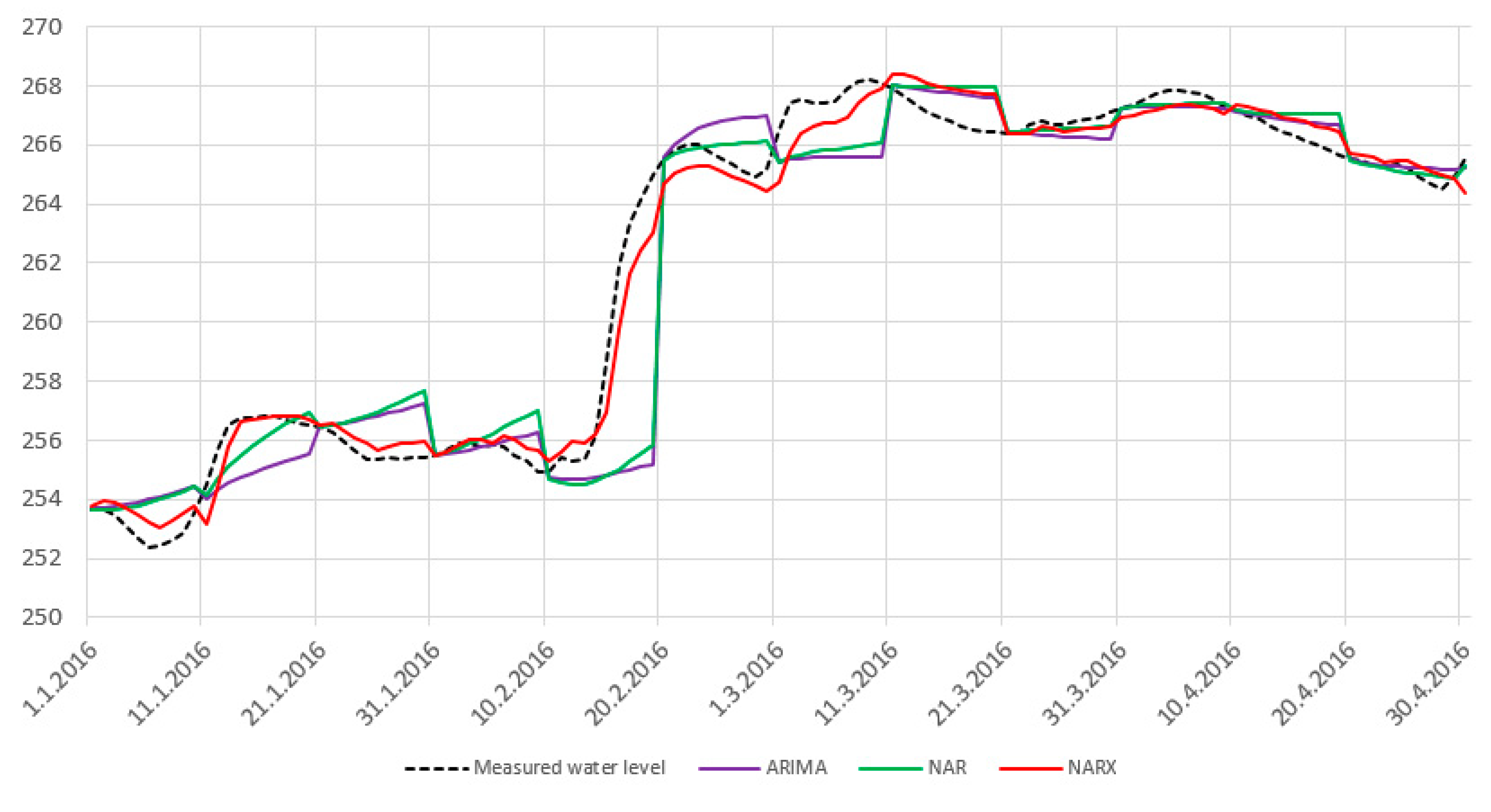In [17] it was concluded that the main weakness of single variable time series water level prediction by NAR networks and FFBP networks is slow adjustment to sudden water level changes. This weakness causes large maximal errors in this prediction method.

External validation is performed to compare the prediction power of three used methods. The data from 1 January 1998 to 7 April 2017 was used for ANN training and ARIMA model fitting and external validation is performed sequentially ten by ten days on the data from 1 January 2016 to 4 January 2017 (37 sequential validations in total). In every sequential step of external validation training/fitting set of data was updated by adding new measured data. The basic principle of sequential approach for short-term prediction is presented in Figure 9.

Among all tested ARIMA models and ANNs structure the best results were obtained by ARIMA (3,0,4) model, NAR network with seven neurons in hidden layer and three delays and NARX network with four neurons in hidden layer and one delay. The results of external validation are presented in

Table 4. External validation results of water level prediction (unit: m).

Method	Input	MAE	MAE 10th Day 1	MAX
ARIMA	Water level	0.90	1.59	9.79
NAR	Water level	0.87	1.57	8.60
NARX	Water level, total water inflow, water discharge, water consumption for the production of electric energy	0.48	0.63	2.13

¹ “MAE 10th day” disregards prediction errors of all the days prior 10th day in sequential approach for short-term prediction.

.

According to data in Table 4, NARX networks outperformed ARIMA and NAR networks in predicting water level in the reservoir. By analysing graph of measured and predicted values of water level by every method it is obvious that this advantage for NARX networks comes in periods when sudden water level occurs. In periods when water level is slowly changing there is no significant difference in prediction quality among tested methods, as presented in Figure 10.

For the prediction of water level for the dam displacement prediction validation series, i.e., for prediction of water level for 23 February 2017 and 7 April 2017 training/fitting data set was updated and three best models/structures of every used method were used for prediction. The mean value of three predictions of every method was used. Results are presented in

Table 5. Water level prediction (unit: m; date format: day/month/year).

Method 1	Prediction for 23.02.2017.	Method	Prediction for 07.04.2017.
ARIMA (3,0,4)	251.72	ARIMA (3,0,4)	260.30
ARIMA (2,0,1)	251.47	ARIMA (2,0,1)	260.23
ARIMA (6,0,1)	251.75	ARIMA (6,0,1)	260.29
NAR (n = 7, d = 3)	250.52	NAR (n = 7, d = 3)	260.56
NAR (n = 6, d = 5)	251.10	NAR (n = 6, d = 5)	260.74
NAR (n = 5, d = 3)	250.87	NAR (n = 5, d = 3)	260.74
NARX (n = 4, d = 1)	250.63	NARX (n = 4, d = 1)	260.57
NARX (n = 5, d = 1)	250.11	NARX (n = 5, d = 1)	260.35
NARX (n = 7, d = 1)	250.36	NARX (n = 7, d = 1)	260.64

¹ n—number of neurons in hidden layer, d—number of delays.

.

Measured water level on 23 February 2017 was 249.40 m and on 7 April 2017 was 260.09 m. Although, all three tested methods showed good results, NARX networks performed somewhat better, especially in the first validation measurement. These results are in agreement with results obtained in external validation presented in Table 4.

Air temperature has direct and indirect influence on dam movements. Direct impact is only on the dam’s surface due to absorbed solar radiation and indirect impact is through water and concrete temperature due to long-term air temperature’s influence on water and concrete.

Weather forecasters use very sophisticated software, algorithms and various sources of weather data (historical data, satellite imagery) to forecast weather. Even with all these tools, weather forecasters struggle to give accurate forecast for period longer than three days. There is no consensus among weather forecasting professionals about what the maximum number of days is which can be reliably forecasted but most of the practitioners agree that accurate weather forecast is not possible for ten or more days, as shown in Figure 11 [37].

Due to the above-mentioned facts, we did not forecast air temperature but air temperature forecasts are taken from web weather services: AccuWeather [38] and The Weather Channel [39]. The results of air weather forecast for ten days ahead in the first validation series and eight days ahead in second validation series are presented in

Table 6. The results of air temperature forecast (unit: °C, date format: day/month/year).

Date	Measured Air Temperature	accuweather.com Forecast	weather.com Forecast
23.02.2017.	7.1	7.0	9.5
07.04.2017.	9.2	8.0	12.0

.

To compare the prediction power of used methods for water temperature prediction external validation is performed on the data from 1 January 2016 to 4 January 2017. The approach for external validation was the same as for water level data. The results of external validation for short-term water temperature prediction are shown in

Table 7. External validation results of water temperature prediction (unit: °C).

Method	Input	MAE	MAE 10th Day 1	MAX
ARIMA	Measured water temperature	0.2	0.4	1.6
NAR	Measured water temperature	0.2	0.3	1.1
NARX	Measured water temperature, measured air temperature	0.2	0.3	1.0

¹ “MAE 10th day” disregards prediction errors of all the days prior 10th day in sequential approach for short-term prediction.

.

The results of external validation showed that there is no significant difference in short-term water temperature prediction among three tested methods. Due to the slow pace of water temperature change, univariate methods are able to adapt and accurately predict future values of water temperature. Hence, no significant difference was detected in accuracy among univariate and multivariate methods when the value of predicted variable changes slowly.

Water temperature prediction is performed by two approaches: the first approach is a simple univariate TSP based on historical water temperature data (ARIMA and NAR networks) and the second approach is multivariate TSP—water temperature is predicted by using measured air temperature, water temperature data and weather forecast air temperature (NARX networks). To predict water temperature on 23 February 2017 and 7 April 2017 three models of each method which showed best results in external validation were used. The mean value of three predictions of every method was used as the final result. Results are presented in

Table 8. Water temperature prediction (unit: °C; date format: day/month/year).

Method 1	Prediction for 23.02.2017.	Method	Prediction for 07.04.2017.
ARIMA (2,0,6)	6.1	ARIMA (2,0,5)	8.7
ARIMA (2,0,7)	6.1	ARIMA (2,0,6)	8.8
ARIMA (7,0,3)	5.9	ARIMA (2,0,7)	8.8
NAR (n = 2, d = 7)	6.3	NAR (n = 2, d = 7)	8.0
NAR (n = 3, d = 7)	5.5	NAR (n = 3, d = 7)	7.9
NAR (n = 4, d = 5)	6.2	NAR (n = 4, d = 5)	8.7
NARX (n = 7, d = 1)	5.7	NARX (n = 7, d = 1)	7.4
NARX (n = 8, d = 1)	6.7	NARX (n = 8, d = 1)	8.2
NARX (n = 9, d = 1)	5.7	NARX (n = 9, d = 1)	8.6

¹ n—number of neurons in hidden layer, d—number of delays.

.

All three used methods predicted accurately measured water temperature on 23 February 2017 (5.9 ℃) and 7 April 2017 (8.6 ℃). Although, prediction errors are small these results are not surprising because water temperature changes slowly and it is not hard to perform short-term prediction.

External validation for concrete temperature is performed on the data from 1 January 2016 to 4 January 2017 by using the same approach as for water level and water temperature data. Results are presented in

Table 9. External validation results of concrete temperature prediction (unit: °C).

Method	Input	MAE	MAE 10th Day 1	MAX
ARIMA	Measured concrete temperature	0.2	0.2	1.1
NAR	Measured concrete temperature	0.2	0.4	1.1
NARX	Measured concrete temperature, measured water temperature, measured air temperature	0.2	0.3	0.7

¹ “MAE 10th day” disregards prediction errors of days prior to 10th day in sequential approach for short-term prediction.

.

The results of concrete temperature prediction were very similar to those from water temperature prediction. These variables change slowly hence univariate prediction had similar accuracy as multivariate prediction.

Concrete temperature prediction was performed by two approaches: the first approach is simple univariate time series prediction based on historical measured concrete temperature data (ARIMA and NAR networks) and the second approach is a two-step cascade approach (NARX networks). Two-step cascade approach has the following form:

• In the first step, water temperature is predicted by using measured and weather forecast air temperature data and measured water temperature data,
• In the second step, measured air temperature, water temperature and concrete temperature, weather forecast air temperature and predicted water temperature from the first step is used for concrete temperature prediction.

For prediction of concrete temperature for two dam displacement prediction validation series (ten days ahead and eight days ahead prediction), training/fitting data set was updated and three best models/structures of every used method were used for prediction. The mean value of three predictions of every method is used as the final result as presented in

Table 10. Concrete temperature prediction (unit: °C; date format: day/month/year).

Method 1	Prediction for 23.02.2017.	Method	Prediction for 07.04.2017.
ARIMA (2,0,1)	8.9	ARIMA (2,0,1)	11.8
ARIMA (2,0,2)	8.9	ARIMA (2,0,2)	11.8
ARIMA (2,0,8)	8.8	ARIMA (2,0,8)	12.0
NAR (n = 4, d = 5)	8.4	NAR (n = 4, d = 5)	12.0
NAR (n = 4, d = 15)	9.1	NAR (n = 4, d = 15)	11.8
NAR (n = 10, d = 7)	8.7	NAR (n = 10, d = 7)	11.8
NARX (n = 2, d = 2)	8.9	NARX (n = 2, d = 2)	11.6
NARX (n = 4, d = 2)	8.9	NARX (n = 4, d = 2)	11.6
NARX (n = 5, d = 1)	8.7	NARX (n = 5, d = 1)	11.6

¹ n—number of neurons in hidden layer, d—number of delays.

.

Measured concrete temperature on 23 February 2017 was 8.8 °C and on 7 April 2017 was 12.1 °C. All three tested methods accurately predicted concrete temperature and additionally, all models had consistent results.

The completed dam displacement data for every object point was matched with the corresponding values of influencing factors for the days when geodetic measurements were performed. These data sets were then used for ANN training and MLR fitting for each point independently. Additionally, separate models for each object point were developed for dam movements in direction of X and Y axes. The main criteria for choosing optimal model for prediction of dam displacements was multiple correlation coefficient R. Correlation test results are presented in Figure 12.

This figure indicates that there is a strong correlation between dam displacements and values of water level in reservoir, air temperature on the dam, reservoir water temperature and dam’s concrete temperature. Additionally, these influencing factors have a larger impact on dam displacements in the direction of X axes (+X upstream, −X downstream) compared to displacements in the direction of Y axes. Also, the results showed that this relationship is not linear for majority of dam object points but if we consider only dam movements in direction of X axes for all object points distanced from dam foundations there is a strong linear correlation between influencing factors and dam movement.

To test predictive power of ANNs and MLR for short-term dam movement prediction based on time series prediction of influencing factors two validation measurements were used. Predicted values of influencing factors were used as an input for trained ANN models with highest R values. A total of 12 combinations were tested, three inputs (ARIMA, NAR and NARX predictions of influencing factors) and four models of displacement prediction (FFBP, CFBP, LRBP and MLR), to investigate the existence of superior combination for prediction. Prediction results for all 12 tested combinations is presented in Appendix A. The results of external validation for short-term dam movement prediction based on time series prediction of influencing factors are presented in

Table 11. External validation for dam movement prediction in direction of X axes (unit: mm).

Method	Input 1	1st Validation MAE	1st Validation MAX Error	2nd Validation MAE	2nd Validation MAX error
CFBP	ARIMA	0.8	1.7	0.5	1.4
CFBP	NAR	0.8	1.9	0.5	1.6
CFBP	NARX	0.8	1.9	0.5	1.5
FFBP	ARIMA	0.7	1.4	0.6	2.1
FFBP	NAR	0.7	1.6	0.7	1.9
FFBP	NARX	0.8	2.0	0.7	1.9
LRBP	ARIMA	0.7	1.6	0.6	1.9
LRBP	NAR	0.7	1.8	0.7	2.1
LRBP	NARX	0.8	1.9	0.7	2.0
MLR	ARIMA	0.4	1.2	0.3	0.9
MLR	NAR	0.5	1.3	0.4	1.1
MLR	NARX	0.6	1.4	0.5	1.1

¹ Method used for prediction of influencing factors which are later used as inputs for the dam movement prediction.

and

Table 12. External validation for dam movement prediction in direction of Y axes (unit: mm).

Method	Input 1	1st Validation MAE	1st Validation MAX Error	2nd Validation MAE	2nd Validation MAX Error
CFBP	ARIMA	0.6	2.1	0.9	2.0
CFBP	NAR	0.7	2.1	0.9	2.4
CFBP	NARX	0.7	2.1	1.0	2.4
FFBP	ARIMA	0.5	1.3	0.9	2.0
FFBP	NAR	0.5	1.5	0.9	2.4
FFBP	NARX	0.6	1.7	1.0	2.4
LRBP	ARIMA	0.5	1.5	1.0	2.5
LRBP	NAR	0.6	1.7	1.1	2.5
LRBP	NARX	0.6	1.7	1.0	2.5
MLR	ARIMA	0.7	1.5	0.8	1.5
MLR	NAR	0.7	1.6	0.9	1.6
MLR	NARX	0.7	1.6	0.9	1.5

¹ Method used for prediction of influencing factors which are later used as inputs for the dam movement prediction.

.

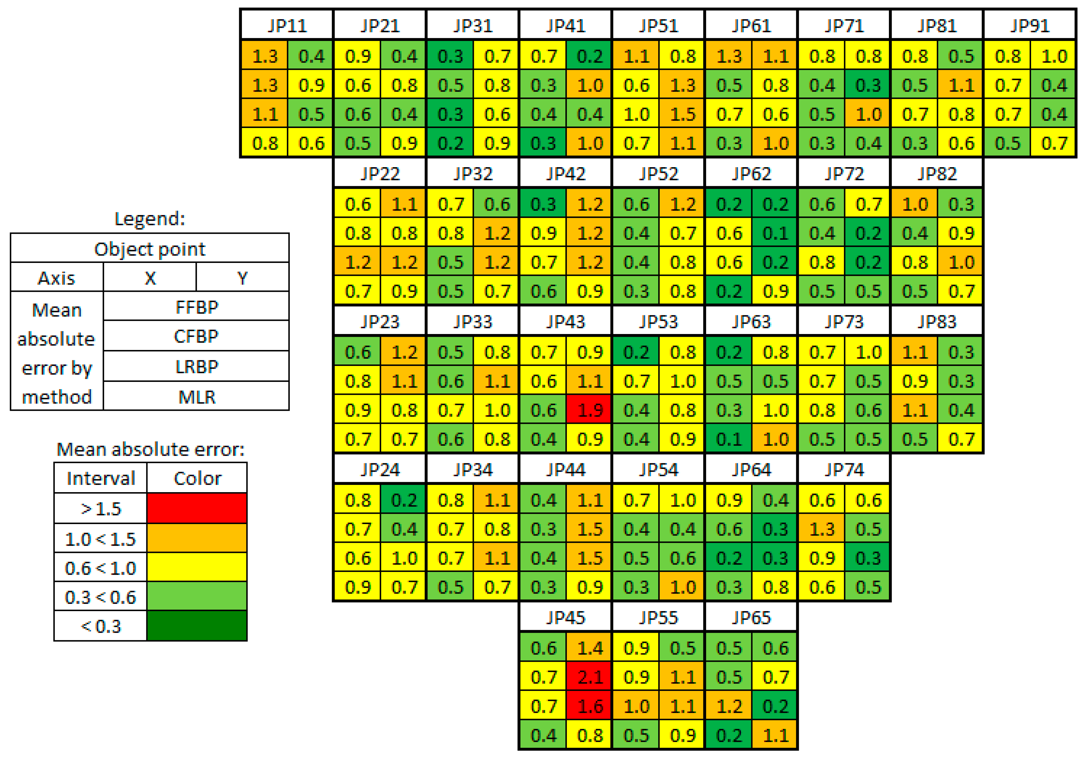
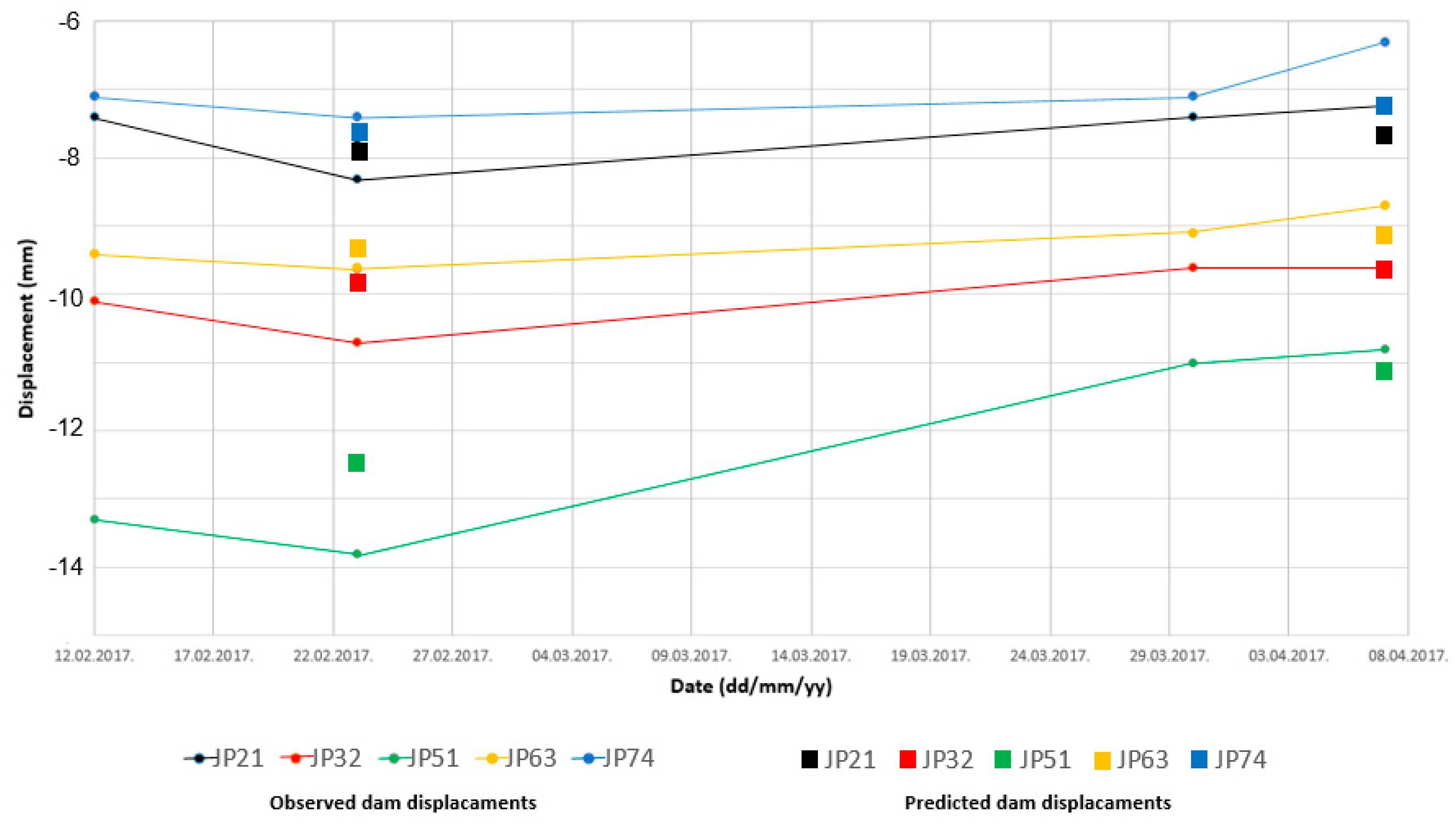
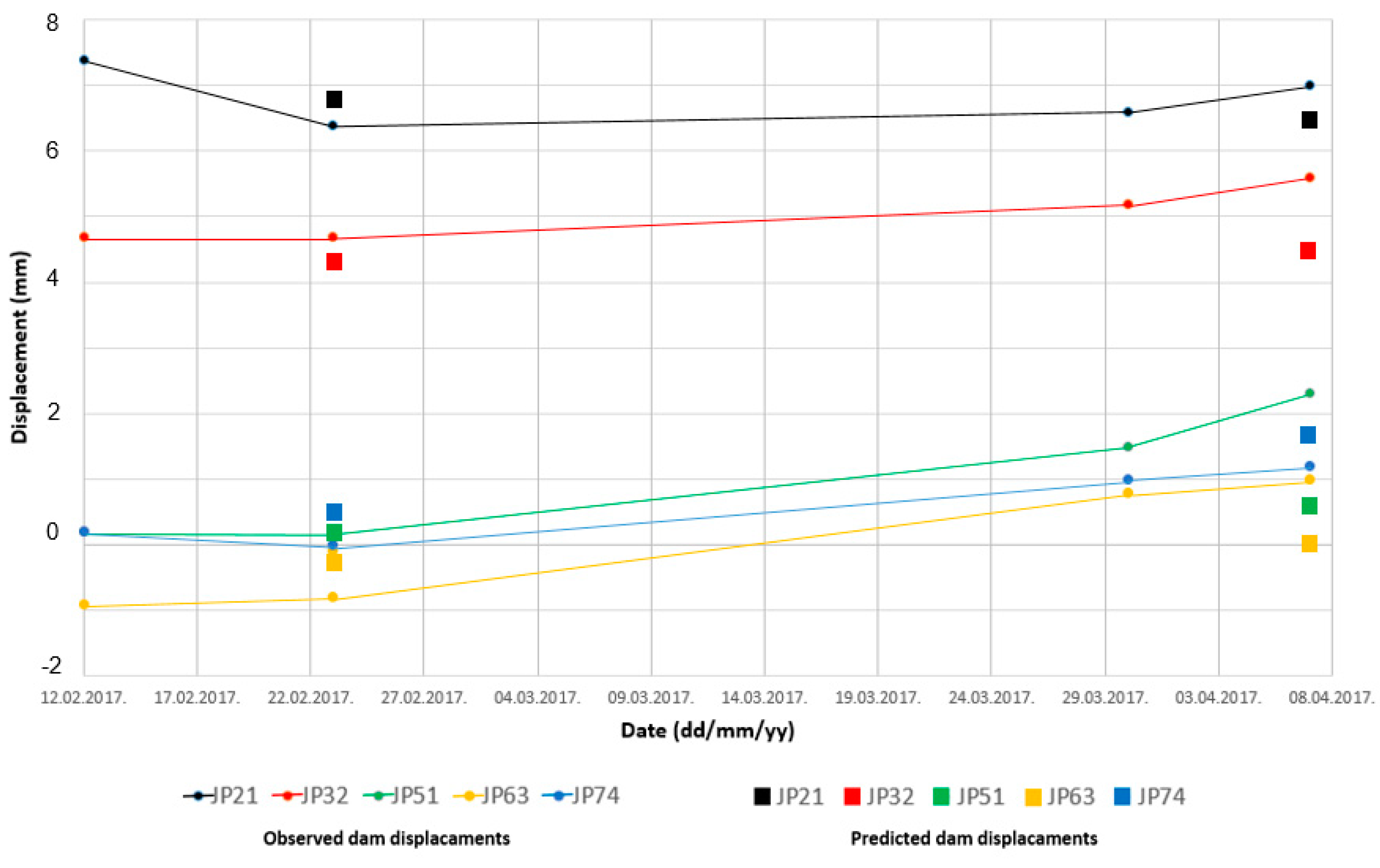
The spatial distribution of the prediction quality for all object points on the dam body is presented in Figure 13. If we consider only dam movements in the direction of the X axes (direction of river flow) it can be concluded that object points distanced from dam foundations have smaller prediction errors compared to those close to the foundations. When considering dam movements in direction of Y axes there is no clear rule that can explain spatial distribution of prediction errors. Additionally, even when correlation coefficients are not very high, for example point JP24, prediction accuracy is still good. Relationship between observed and predicted deformations for five selected object points in four consecutive measurement series is presented in Figure 14 and Figure 15. Predicted dam displacement is mean value of predictions from all used methods.

As it can be seen from Figure 14 and Figure 15, the proposed approach for dam movement prediction can accurately estimate dam movement on every part of the object. Also, predicted values of dam displacements often follow the current trend of dam movements in directions of X and Y axes.

By analysing all obtained results, it can be concluded that by using proposed approach it is possible to accurately predict short-term dam movement based on predicted values of influencing factors. There was no single combination which showed superior prediction results compared to other tested methods but MLR showed somewhat better results compared to ANNs in both validation series for prediction of dam movement in direction of X axes. This result is counterintuitive because ANNs performs better (scored higher R values) when testing ANNs and MLR models.

4. Conclusions

In this research, complete process of data acquisition, data processing and dam stability analysis by means of geodetic measurements are presented. Four major influencing factors for short-term dam movement are identified and later used for short-term movement prediction.

A method based on ANNs for the interpolation of missing dam displacement data is presented and used for the completion of missing dam displacement data. This unique method had sufficient accuracy for predicting missing dam displacement data which is confirmed by external validation on four known object points.

Time series prediction of influencing factors is performed by a statistical method (ARIMA) and two machine learning methods (NAR network and NARX network). Two approaches were presented for the prediction of time series influencing factors. The first approach uses only historical data of predicted variable. The second, multivariate method, approach which cascade prediction taking in account interdependence of influencing factors. External validation was performed to compare used methods and approaches sequential. The results show that multivariate prediction of water level is superior to univariate prediction. This superiority is especially noticeable in periods of sudden changes in water level. In periods when water level changes slowly univariate and multivariate prediction shows very similar results. Water temperature in reservoir and concrete temperature of the dam changes slowly and in these particular examples there was no significant difference in prediction accuracy among three tested methods.

To inspect the existence of correlation between influencing factors and dam displacements three types of classical ANNS (FFBP, CFBP and LRBP) and a statistical method (MLR) were used. As a measure of predictive power multiple regression coefficient (R) is used. The results show that there is significant relationship between selected influencing factors and dam movements. Calculated R coefficient from MLR proved that this relationship is not linear for most of object points but at the same time this simple statistical method shows good results for short-term prediction of dam displacements based on predicted values of influencing factors.

Very high values of R for all three tested ANNs show that ANNs can correctly generalise dam movement based on values of influencing factors. This is the most important result of this research because object health state can be determined by comparing measured values of dam displacements and predicted values obtained by ANNs prediction based on measured influencing factors. Measured and compared values must agree with low residuals, otherwise some external factor (geological instability, internal erosion, dam material decay) caused unexpected dam movement.

All four used methods for short-term dam movement based on predicted values of influencing factors indicated good prediction results. The main limiting factor for extending prediction length is accurate long-term weather forecast, especially accurate precipitation which exerts a direct influence on water level and air temperature that further influence water and concrete temperature.

The results obtained in this research could be improved by adding new data in used models, e.g., new monitoring series of measurements. A good chance of improving prediction of water level data exists by calculating water catchment area for all rivers and streams that influence total water inflow in reservoir. This could be accomplished by using digital terrain model. By adding measured precipitation and forecasted precipitation data water level prediction could be improved. This is significant factor for dam movement prediction and if calculated with high accuracy these data could also be used for planning production of electric energy. Additionally, remote sensing data (historical and actual) could be used to better understand dam behaviour in relation with influencing factors. By installing GPS receivers on the dam crest, it would be possible to assess state of the dam’s health in real time and investigate how influencing factors effect dam’s movement. These could be future tasks for the research and guidelines for improving dam monitoring system.