Article

Quantitative Evaluation of Spatial Differentiation for Public Open Spaces in Urban Built-Up Areas by Assessing SDG 11.7: A Case of Deqing County

School of Geomatics and Urban Spatial Information, Beijing University of Civil Engineering and Architecture, Beijing 102616, China
*
Author to whom correspondence should be addressed.
ISPRS Int. J. Geo-Inf. 2020, 9(10), 575; https://0-doi-org.brum.beds.ac.uk/10.3390/ijgi9100575
Submission received: 20 May 2020 / Revised: 16 September 2020 / Accepted: 28 September 2020 / Published: 30 September 2020

Abstract

:
Urban public open spaces refer to open space between architectural structures in a city or urban agglomeration that is open for urban residents to conduct public exchanges and hold various activities. Sustainable Development Goal (SDG) 11.7 in the 2030 UN Agenda for Sustainable Development clearly states that the distribution characteristics of public open spaces are important indicators to measure the sustainable development of urban ecological society. In 2018, in order to implement the sustainable development agenda, China offered the example of Deqing to the world. Therefore, taking Deqing as an example, this paper uses geographic statistics and spatial analysis methods to quantitatively evaluate and visualize public open spaces in the built area in 2016 and analyzes the spatial pattern and relationship of the population. The results show that the public open spaces in the built-up area of Deqing have typical global and local spatial autocorrelation. The spatial pattern shows obvious differences in different parts of the built area and attributes of public open spaces. According to the results of correlation analysis, it can be seen that the decentralized characteristics of public open spaces have a significant relationship with the population agglomeration, and this correlation is also related to the types of public open spaces. The assessment results by SDG 11.7.1 indicate that the public open spaces in the built-up area of Deqing conform to the living needs of residents on the whole and have a humanized space design and good accessibility. However, the per capita public open spaces of towns and villages outside the built area are relatively low, and there is an imbalance in public open spaces. Therefore, more attention should be paid to constructing urban public open spaces fairly.

1. Introduction

In 2015, the UN Development Summit approved and adopted the 2030 Agenda for Sustainable Development, which sets out 17 Sustainable Development Goals (SDGs) covering three major areas, economic, social, and environmental, charting a course for the development of countries and international cooperation. The primary task of a comprehensive assessment of the practice of SDGs in a region is to localize the UN SDGs global indicator framework. At the first United Nations World Geospatial Information Congress in 2018, China released a quantitative assessment report “Deqing Practice Report on the Implementation of the 2030 Sustainable Development Agenda (2017)”. The report shows that most indicators of Deqing, Zhejiang, are close to the UN 2030 Sustainable Development Goals. Based on the SDG global indicator framework and geographic statistical information, the project team carried out a localized evaluation and analysis of the implementation of Deqing County, combining quantitative, qualitative, and localization data [1,2], and offered the Deqing sample to the international community.
The 2030 Agenda for Sustainable Development aims to comprehensively address the three dimensions of development (social, economic, and environmental) from 2015 to 2030, and shift to a sustainable development path. Especially, SDG 11 promotes the construction of tolerant, secure, disaster-proof, and sustainable cities and human settlements, with a focus on improving living conditions, optimizing the habitable environment, and ensuring the safety of houses. In Deqing, the aspects of inclusivity, sustainability, and disaster resistance comprehensively reflect the county’s progress in the practice of creating a sustainable city and human settlements. SDG 11 contains 10 quantitative indicators, of which indicator 11.7 is the universal provision of safe, inclusive, accessible, and green public spaces to all people, especially women, children, the elderly, and people with disabilities. The aim of SDG 11 is to analyze the proportion of public spaces per capita to reflect livable environmental conditions. Combining SDG 11.7 with the actual situation of Deqing, and considering the availability and quantitative characteristics of the data, this paper focuses on urban built-up areas, analyzes the average proportion of public open spaces used by all, and provides a guarantee for the construction of urban public open spaces that can meet everyone’s needs.
Having enough public space enables cities and regions to function efficiently and fairly [3]. Reduced public space has a negative impact on quality of life, social inclusion, infrastructure development, environmental sustainability and productivity. It has been recorded that good design and maintenance of streets and public spaces can reduce crime and violence, improve the quality of residents’ lives and the overall appearance of the city, and play a very important role in beautifying the image of the city [4]. At the same time, the ratio of urban streets to public spaces is an important feature of urban space planning, and cities with sufficient streets and public spaces and greater connectivity are more livable and productive [5]. Planning sufficient space for critical infrastructure sites such as water resources, sewers and waste collection, recreational spaces, green spaces and parks can help strengthen social cohesion and protect green, ecologically sustainable development. Making enough space to support formal and informal economic activities [6], actively restoring and maintaining public spaces for various users, and providing services and opportunities for marginalized residents are all conducive to enhancing social cohesion and economic security.
Considering the impact of urban public open spaces on sustainable development, many scholars have conducted qualitative and quantitative analyses of urban public spaces at different levels and from multiple perspectives [7]. Scholars have made extensive studies on modern urban planning and landscape design [8,9], social perspectives [7], spatial distribution and quality assessment [10], etc. Qualitatively and quantitatively, different suggestions have been put forward for creating popular and ecological urban public open spaces, which enriches the construction concept of urban public spaces. Other scholars have conducted many studies on the equity of public space allocation [11,12,13]. They evaluated and analyzed urban income, race, social economy, and other aspects, and advocated for the importance of environmental equity, which contributes to reducing the inequality of urban public spaces. However, few scholars have carried out spatial differentiation law analysis of all components of urban public open spaces, and most studies were confined to parts of public spaces, such as parks, squares, and green spaces, to carry out spatial distribution analysis and environmental assessment separately [3,14]. The spatial distribution of public open spaces in terms of society, history, transportation, economy, and population was studied from multiple perspectives, but faced with the rapid development of urbanization today, solving the problem of public spaces in crowded areas has become a hot spot. There is an urgent need to improve residents’ quality of life, and all elements of public open spaces for the overall analysis to improve the safe and healthy life of residents are important.
According to the existing research results, the important index for evaluating urban public open spaces is the spatial pattern and formation mechanism. Generally speaking, evaluating the spatial pattern mainly involves quantitative analysis of the distribution form, agglomeration degree, and agglomeration mode of urban elements in order to describe the spatial clustering and stratum distribution characteristics of the space. The formation mechanism of urban public open spaces is related to the urban spatial structure system, public facilities factors, and distribution and intensity of human activities. Therefore, we want to use geographic information system (GIS) spatial autocorrelation analysis to describe the differences in urban public open spaces distribution, and use hot spot and overlay analysis to explore the driving factors that affect the formation of urban public open spaces.
In recent years, many scholars have used GIS spatial analysis to carry out research on urban spatial pattern analysis. Shirowzhan [15] proposed two classification algorithms that are based on spatial autocorrelation statistics, such as the Local Moran’s I and the Getis-Ord Gi*, which are computed over sample urban areas including complex terrain with diverse building characteristics, and used these algorithms to airborne lidar point clouds over the complex urban areas in order to generate highly accurate DEMs and classify the lidar points. Aghajani [16] proposed a road accident analysis method, which operates through the use of the GIS spatial and temporal patterns in urban road accident prone locations; he also used the hot spot analysis with identification and data generation to help decision makers to take appropriate measures to decrease road accidents. Fan [17] used the local spatial autocorrelation to characterize urban landscape fragmentation, and he compared two local spatial autocorrelation indices, the Getis statistic and the local Moran’s I, to evaluate the landscape pattern. Xia [18] used the local indicator of spatial association to analyze the spatial relationships between urban land use intensity and urban vitality, and they found that there is a significant positive spatial autocorrelation between urban land use intensity and urban vitality according to global statistics. Shen [19] used both global and local spatial autocorrelation analyses to demonstrate how urban sustainability was spatially distributed across neighborhoods and what patterns (random, dispersed, or clustered) could be statistically identified. Majumdar [20] used the local Moran’s I to recognize the pattern of statistically significant LST increase by detecting clusters of localized hot spots. Some scholars also used the spatial autocorrelation analysis in the field of river network monitoring [21], spatial variations analysis of NPP [22], and agricultural spatial relationship analysis of drought propagation [23]. According to these kinds of research results, we found that GIS spatial analysis methods can help us to identify the spatial pattern among kinds of urban objects, but most of their research only used the local indicators of spatial association (LISA) to judge the relationship between these events (such as road accident, land use classification, river network monitoring, and soon on) in urban environment, and lacked a quantitative description of the causes of these events. The aim of our research is not only to find the spatial pattern, but also to quantitatively analyze the formation of urban public open spaces.
Above all, public space is an indispensable component in the city. In view of all elements of public space being integral to the analysis, this paper is based on SDG 11.7, in combination with the practical situation of Deqing and existing data, adopting the method of geographic statistics and GIS spatial analysis of Deqing public open spaces for spatial differentiation pattern. Furthermore, the population data are analyzed to provide a quantitative assessment of and technical support for the sustainable development goal of building safe, inclusive, barrier-free, and green public open spaces in Deqing. It provides decision support for the management and planning of public open spaces.

2. Materials and Methods

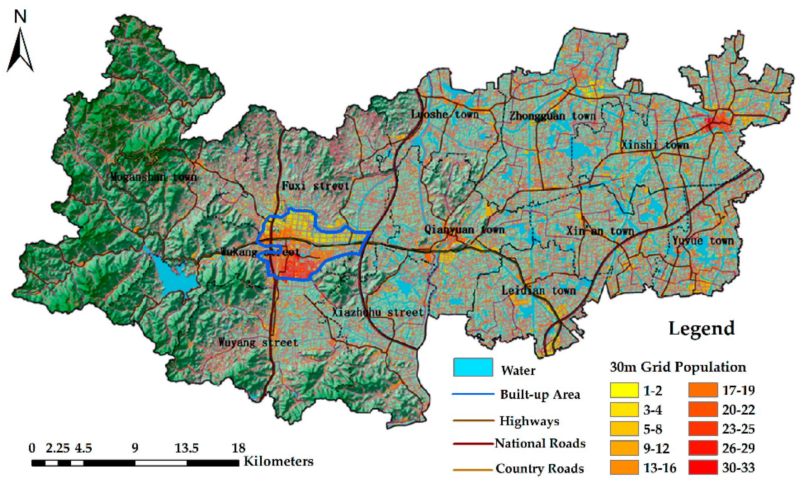
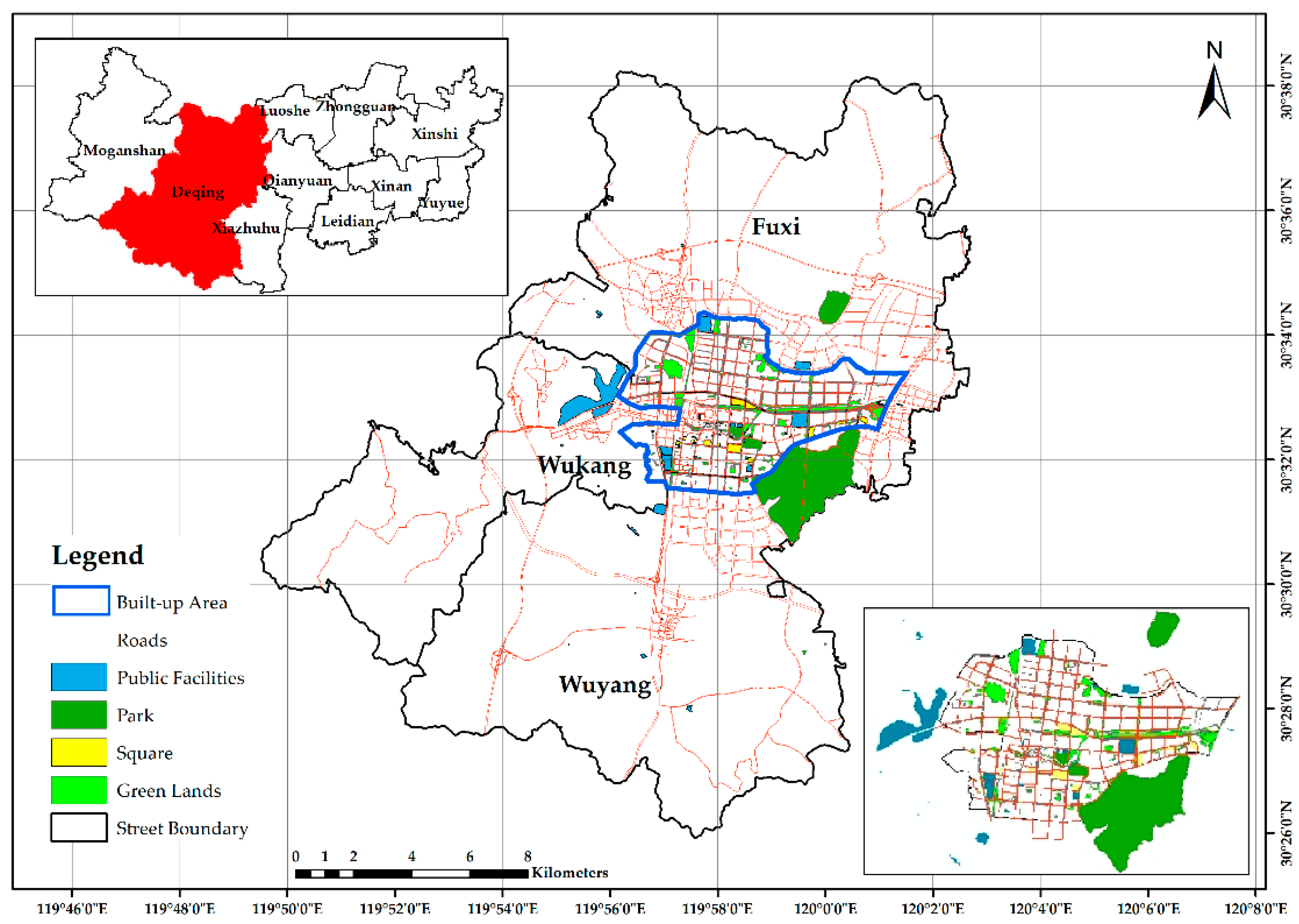
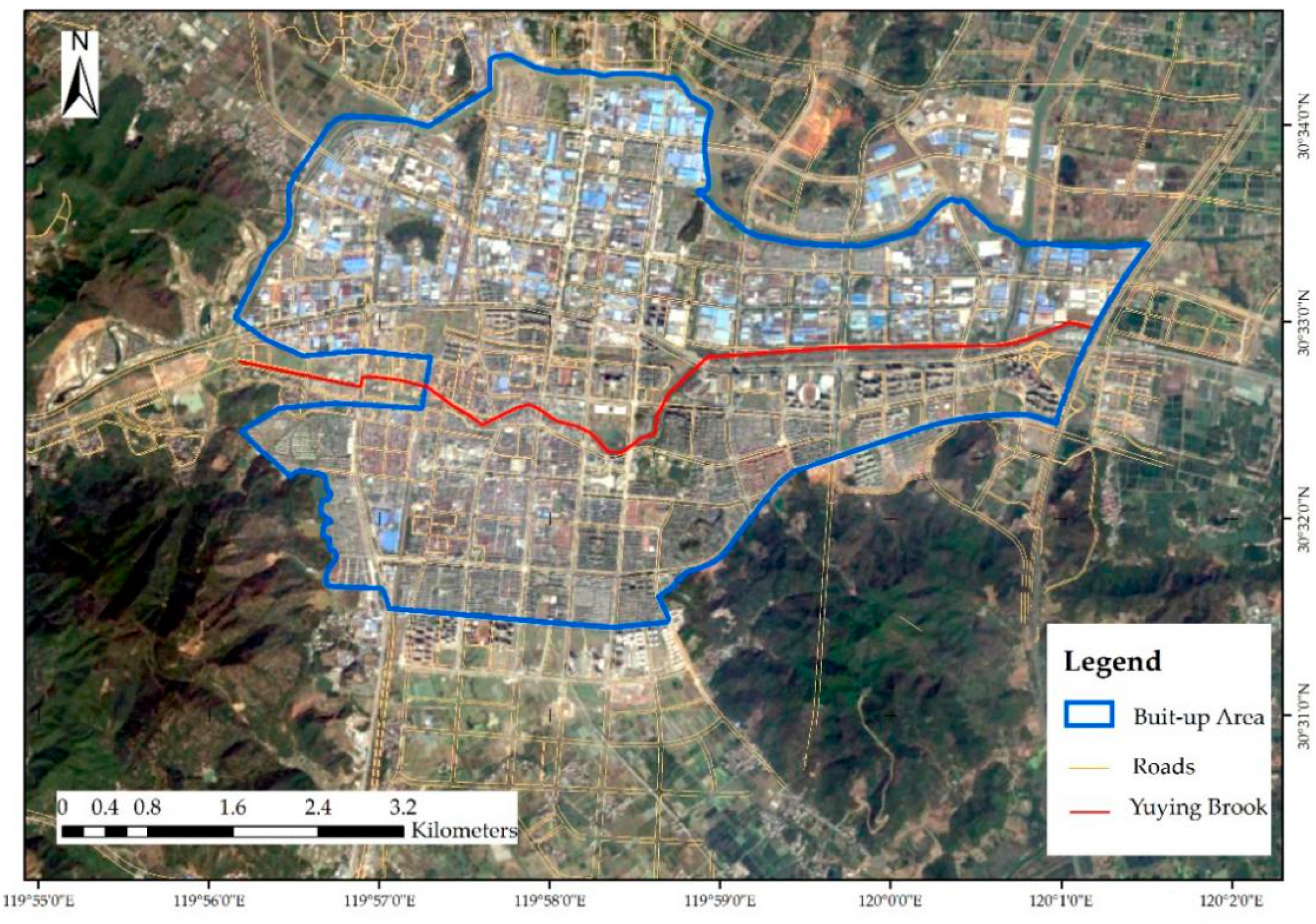
2.1. Study Area and Data

Deqing is a small county in Huzhou City, Zhejiang Province, China. It is located in the north of Zhejiang and consists of 9 towns and 2 townships, and the total area is 937.92 km2 (Figure 1). In 2016, Deqing County was listed among the top 100 counties with the highest comprehensive strength of China’s small and medium-sized cities. The public open spaces of built-up areas and 3 streets or districts (Wuyang, Fuxi and Wukang) were extracted from the remote sensing images taken in 2016, with 0.5m spatial resolution (Figure 2). Yuying brook runs though the downtown of Deqing (red line in Figure 2). The remote sensing image presents true color synthesis product data provided by the Geomatics Center of Deqing. It was made based on Google Earth, and it was shot on 11th, March 2017.
There are four types of public open spaces in Deqing, which are park, square, green land, and public facilities. Because urban public spaces in Deqing are mainly distributed in the built-up area (the blue polygon in Figure 1), what we are mostly concerned with is also the built-up area in Deqing. It needs to be pointed out that there are large forest parks and a golf course in the southeast and west of the built-up area, respectively. These two areas are not within the built-up area, but it is also worthwhile to analyze their autocorrelation effect on the distribution of public space in the built-up area, so we called these areas ‘edge areas’ in this paper. In the autocorrelation analysis of public open spaces in Deqing, we will analyze the whole area and the built-up area separately.
The population of Deqing in 2016 is 440,000 (The population data is from the “Urban Construction Statistical Yearbook of Zhejiang Province (2016)”) and these data were gridded into a raster layer by the Geomatics Center of Deqing (Figure 3), and these data were used to analyze the correlation between the urban public space distribution and population aggregation in Section 3.3 and Section 4.3.

2.2. Methods

Spatial autocorrelation analysis is a technique to test whether the observed values of an element with spatial location are significantly correlated with the observed values at adjacent spatial points, and it is a technique for calculating the degree of spatial unit attribute aggregation [24,25]. In this paper, we analyzed the spatial distribution characteristics and formation mechanism of urban public open spaces at the global and local levels. Global autocorrelation analysis mainly describes the overall distribution of urban public open spaces and determines whether the phenomenon has aggregation characteristics within the city, but it does not indicate exactly where the aggregation areas are. Local autocorrelation analysis mainly judges whether there is a significant aggregation area or spatial hot spot, and calculates the range of the spatial hot spot. In addition, we used population data as the main influence factor, combined with hot spot analysis and geographically weighted regression methods, to analyze the relationship between public open spaces and the population.

2.2.1. Global Spatial Autocorrelation Analysis

Global spatial autocorrelation refers to the degree of spatial autocorrelation of a single attribute value in the whole research area. The most commonly used correlation indicator is Moran’s I [26,27,28]. In this paper, the global Moran’s I was used to test and determine the global autocorrelation of public open spaces in the built-up area of Deqing and surrounding streets. The calculation formula is as follows:
I G l o b a l M o r a n s = n i = 1 n j = 1 n ω i j ( P i P m e a n ) * ( P j P m e a n ) ( i = 1 n j = 1 n ω i j ) i = 1 n ( P i P m e a n ) 2
where pi and pj are the category i and j areas of public open spaces, respectively, and i and j cannot be equal; ωij represents the space weight matrix between space units i and j; and n is the number of public open spaces.
The variation range of Moran’s I index is (−1,1). If the spatial process is irrelevant, the expected value of I is close to 0; when I is negative, it means negative autocorrelation; and when I is positive, it means positive correlation.
Moran’s I cannot fully reflect the distribution pattern of spatial variables, so it needs to be compared with the I index (expectation and variance) in the random pattern, and then used to construct the z-statistic, which follows the normal distribution, is constructed to test the significance of the spatial autocorrelation of the research variables. The expression of the z-statistic is:
Z = I obs E ( I ) D ( I )
where E(I) and D(I) are the expectation and variance of I, and Iobs is the Moran’s I value calculated from the actual data.

2.2.2. Local Spatial Autocorrelation Analysis

Local spatial autocorrelation is the degree of correlation between a spatial unit and an attribute of its adjacent units. The global autocorrelation index determines the distribution of public spaces, but because of the space data heterogeneity, global autocorrelation data may exist in the local randomness; there is also a global random distribution data of partial correlation, so we used the local indicators of spatial association (LISA) [29] to measure the local correlation of urban public spaces. The calculation formula is:
I i = n ( x i x ¯ ) j = 1 n ω i j ( x j x ¯ ) i = 1 n ( x i x ¯ ) 2
where ωij is the spatial weight coefficient matrix, which is used to express the spatial position relationship between research objects, and can reflect the contribution degree of a public space to an adjacent public space.
In this paper, the area of public space was taken as the spatial weight matrix. The value range of local Moran’s I was not limited to (−1, 1). The spatial association model can be subdivided into 4 types: HH, HL, LH, and LL. HH is the focal point associated with high value and high value, indicating that the public space and a surrounding public space occupy a large area; LL is the focal point of the correlation between low value and low value, indicating that the public space and a surrounding public space occupy a relatively small area. LH and HL have outlined correlation regions, indicating that there is strong heterogeneity between the attributes of public open spaces and the surrounding public space. As in other statistics, the value of local Moran’s I needed to be compared to the expectation and tested with its standardized Z-value.

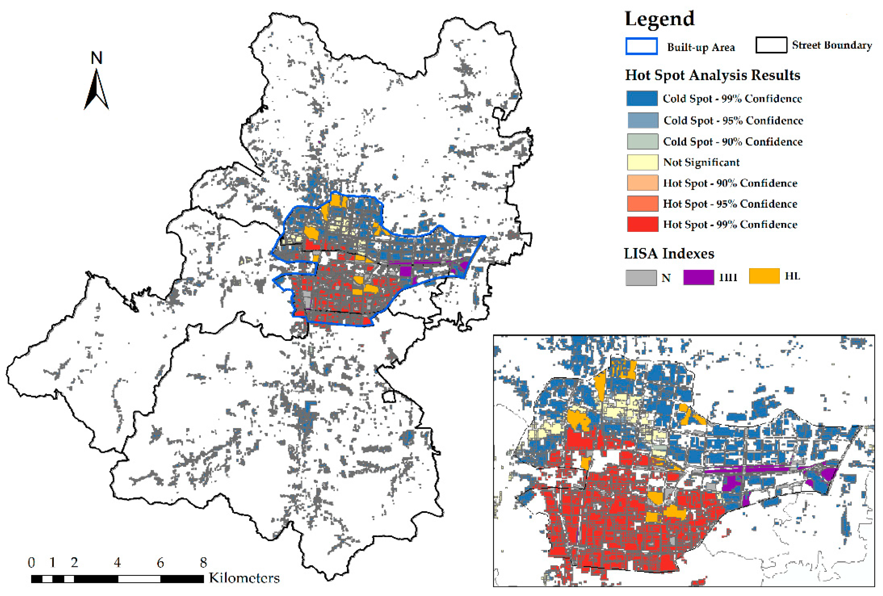
2.2.3. Hot Spot Analysis

Hot spot analysis is used to identify the spatial clustering of high values (hot spots) and low values (cold points) with statistical significance, and a new output factor class is created for each element in the input element class by using z-score, p-value, and confidence interval (Gi_Bin) [30]. If the factor’s z-score is high and p-value is small, then spatial clustering with a high value is indicated. If the z-score is low and negative and the p value is small, there is a spatial clustering with low value. The higher (or lower) the z-score, the greater the clustering degree. If the z-score is close to zero, there is no obvious spatial clustering [31].
In this paper, spatial analysis of population data in the built-up area of Deqing and the surrounding 3 streets (Wuyang, Fuxi, and Wukang) was conducted by using hot spot analysis to judge whether there was an obvious correlation between the clustering characteristics of population distribution and the spatial distribution characteristics of public open spaces in the study area.

2.2.4. Statistics and Evaluation Methods of Urban Public Open Spaces by SDG 11.7

In terms of SDG 11.7 in the UN 2030 Agenda, it said that “By 2030, provide universal access to safe, inclusive and accessible, green and public spaces, in particular for women and children, older persons and persons with disabilities”, and it also provided the assessment indicator of SDG 11.7.1, which is “average share of the built-up area of cities that is open space for public use for all, by sex, age and persons with disabilities”. Area of public open spaces as a proportion of total city space, including the land allocated to streets. The indicator was calculated by integrating two metrics: (a) land allocated to public open spaces; (b) land allocated to streets. The proportion of urban area allocated to public open spaces, including street and sidewalks, was calculated by the following formula:
p = S p + S l S b × 100 %
where P is the proportion of total public open spaces, Sp is the total surface are of public open spaces, Sl is the total surface of land allocated to streets, Sb is the total surface area of the built-up area of the urban agglomeration. So, the method to estimate the area of public open spaces is based on three steps: (1) spatial analysis to delimit the built-up area of the city; (2) estimation of the total public open spaces and; (3) estimation of the total area allocated to streets. Considering that green land is the major part of urban public open spaces, and it could reflect the intensity of urban development, we also recognize the ratio of green land as an indicator of assessment of urban public space.
Ratio of green land (G) in the built-up area is:
G = S g S b × 100 %
where Sg is the total surface area of green land in the built-up area. We used these indicators to measure the sustainable development level of public open spaces in Deqing, and to compare with UN 2030 goals.

2.2.5. Geographically Weighted Regression Model

The geographically weighted regression (GWR) model is a spatial analysis technology—it explores the spatial changes and related driving factors of the research object by establishing a local regression equation at each point, and can be used to predict the future results [32]. In this paper, we used the GWR to show the relation between population and four types of public open spaces.
The general regression model is:
y i = k β 0 + β k x i k + ε i
where y is the dependent variable, x is the independent variable, β is the regression coefficient, and ε is the random error. The GWR is an extension of the traditional regression model so that its parameters can be estimated locally, so the GWR model is:
y i = β 0 ( u i , v i ) + k β k ( u i , v i ) x i k + ε i
where (ui,vi) is the coordinates of the i-th point, and βk(ui,vi) is the value of the continuous function βk(u,v) at i.

3. Results

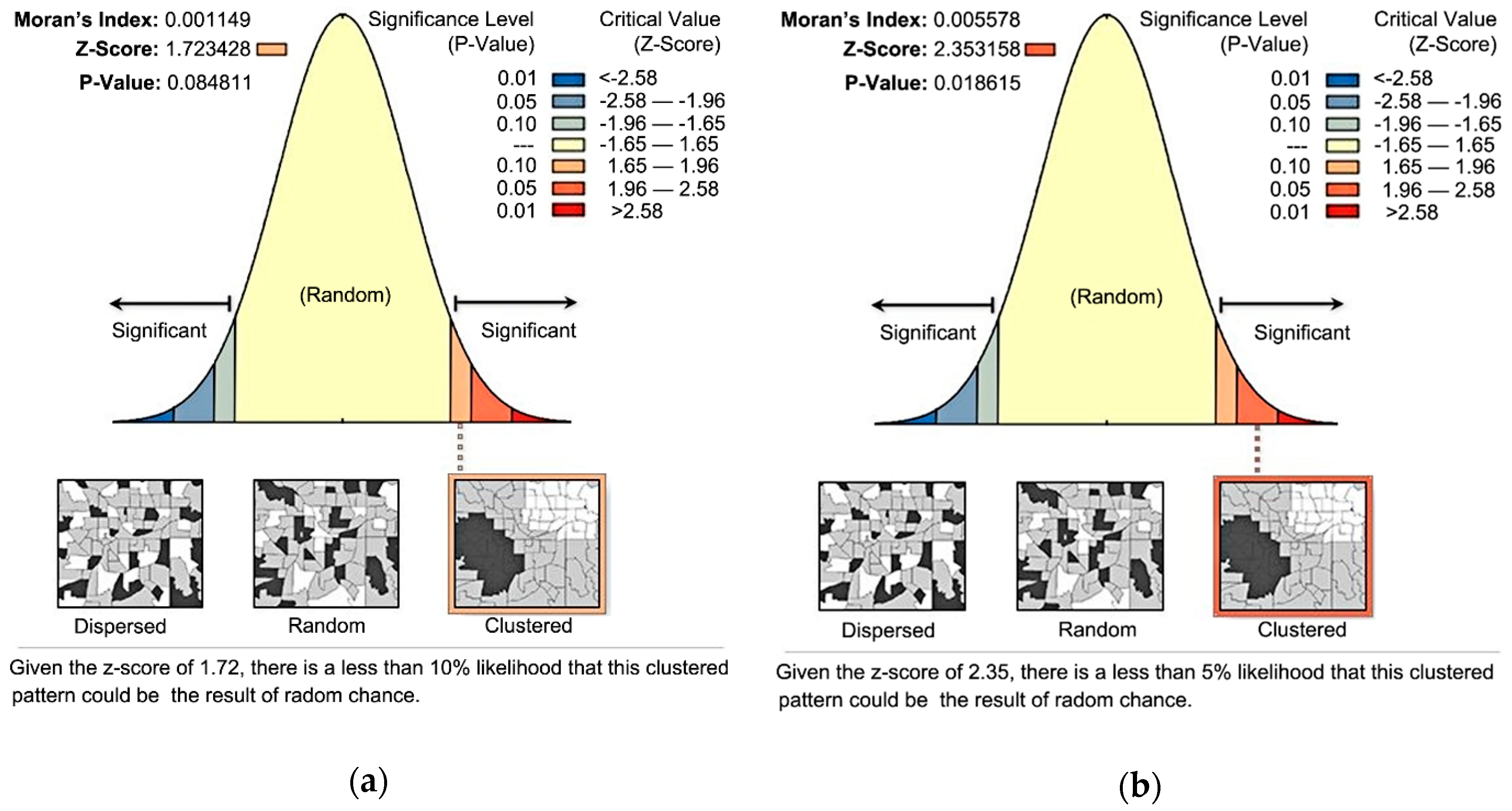
3.1. Analysis of Global Differentiation Pattern

In this paper, global spatial autocorrelation is used to analyze the public open spaces in the built-up area and edge area of Deqing. We analyzed the spatial autocorrelation of the three attributes of urban public space in Deqing, including area, length, and type. The results are shown in Figure 4 and Table 1.
According to the Table 1, we found that the global autocorrelation of public spaces is positive in terms of area, length, and type. Taking the area as an example, the Moran’s I of the whole area is just 0.001149, and one of built-up area has increased to 0.005578, as shown in Figure 4b. The Z-values of the whole area and the built-up area were 1.72 and 2.47, respectively. Z did not fall into the confidence interval [−1.96,1.96], that is, when the significance level was set at 0.05, the public space distribution showed positive spatial autocorrelation. Meanwhile, we found that the autocorrelation of public spaces is more positive and significant in terms of length and type. The Moran’s I and Z-value also increased by removing the edge area from the whole area. It can be seen that the edge area has a great influence on the autocorrelation of public spaces of the built-up area, especially for the analysis of area and length.
The results show that the z-value changes from 1.72 to 2.35 and the spatial autocorrelation of public space is significantly improved after removing the edge area, in terms of area. These two types of public space cover significantly larger areas than other public spaces. This takes advantage of the local regional features in developing tourism and promoting the rapid development of the economy at the same time, but the autocorrelation of the whole public open spaces is weakened due to its distance from the public space in the city. In addition to the edge factors, the public open spaces have obvious clustering characteristics, mainly because Yuying brook runs through the downtown of Deqing, and especially in the downtown area, parks and squares for recreation have been built around the lake. Many green spaces are distributed along the beach of the lake, and the green space beside the park and the built-up area covers the largest area. Public facilities are mainly distributed in the vicinity of residential areas. As can be seen from Figure 1, the further away from the built-up area, the less public space there is. Except for some small public facilities, such as community health centers and temples, parks and squares are rarely distributed. On the whole, there is significant spatial autocorrelation in the public open spaces of the built-up area of Deqing. Setting large leisure areas at the edge of built-up areas not only expands the scope of public space in Deqing City, but also provides enough public open spaces for residents in built-up areas and surrounding towns, and alleviates the crowding of public spaces in built-up areas. This provides a guarantee for a healthy and green life for residents and promotes the sustainable development of the ecological economy in Deqing.

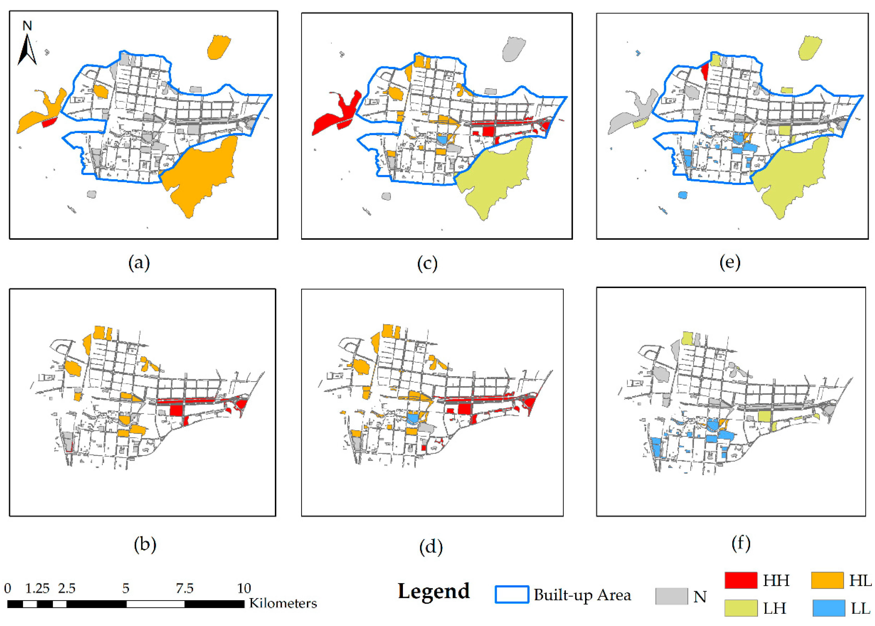
3.2. Analysis of Local Differentiation Pattern

In this paper, the LISA index was used to conduct local spatial autocorrelation analysis of public open spaces in built-up areas and the surrounding edge area in Deqing. The LISA map is shown in Figure 5. The local spatial distribution of public open spaces is characterized by five types, HH (High-High) is a cluster of high values, HL (High-Low) is an accumulation of high and low values, LH( Low-High) is an accumulation of low and high values, and LL (Low-Low) is a cluster of low values, N (Not Significant) represents no significant feature. The HH (LL) area indicates that public spaces with high (low) values have aggregation characteristics, and the HL (LH) area represents the abnormal area caused by public space with a high (low) value surrounded by public space with a low (high) value.
According to the actual situation, due to the existence of public space occupying a large area at the edge area, the local spatial autocorrelation within the built-up area is not normally expressed, as shown in Figure 5a,c,e. Therefore, edge factors were removed for local spatial autocorrelation analysis, and the results are shown in Figure 5b,d,f. From the figure, it can be seen that the red area is the cluster of high values. From the property sheet, it can be seen that the green space with high values has aggregation characteristics. According to the analysis of the geographic environment, the north bank of Yuying brook is mainly a development zone, while the south bank is mainly a development zone and villa area. In terms of traffic, the built-up area is close to the Changshen expressway in the west, where the Linmo line and Changshen expressway are interlinked, and the green space around the traffic line is widely distributed, so it has an obvious high-value clustering feature in the west of Deqing. Under this spatial feature, convenient transportation facilities promoted the rapid economic development of Deqing, and the green land along the river on both sides was conducive to promoting the green and ecological image of the city. The yellow and orange areas are characterized by high and low values, mainly because these areas represent the park and square in the city center and the scenic area near the city. It is surrounded by other public spaces, such as the green belt of the residential area and public facilities, which results in clustering characteristics of high and low values. This distribution feature indicates that the public space design in the built-up area of Deqing is humanized, meets the needs of the public, and is conducive to green, safe, and sustainable healthy living space. The gray areas are mainly urban roads and residential green areas, which are scattered randomly and have no obvious local clustering characteristics. On the whole, public open spaces in the built-up area of Deqing are mainly distributed in the western part of the city (mainly green space), as well as the parks and squares in the inner part of the city and scenic spots on the edge. However, there is very little distribution in other towns outside the built area. This distribution shows the imbalance of public open spaces in the research area. It is necessary to make an equitable improvement plan to promote the overall, balanced and sustainable development of Deqing. Additionally, the length of public open spaces has a similar aggregation with the area, and the aggregation of type is lower than other attributes.
The results of global and local spatial autocorrelation analysis indicate that public open spaces have positive and significant spatial correlation and spatial agglomeration characteristics in space pattern. In addition, different attributes of public space have shown different relevance and aggregation. The type has the most positive and significant global autocorrelation, but it also has the worst local aggregation.

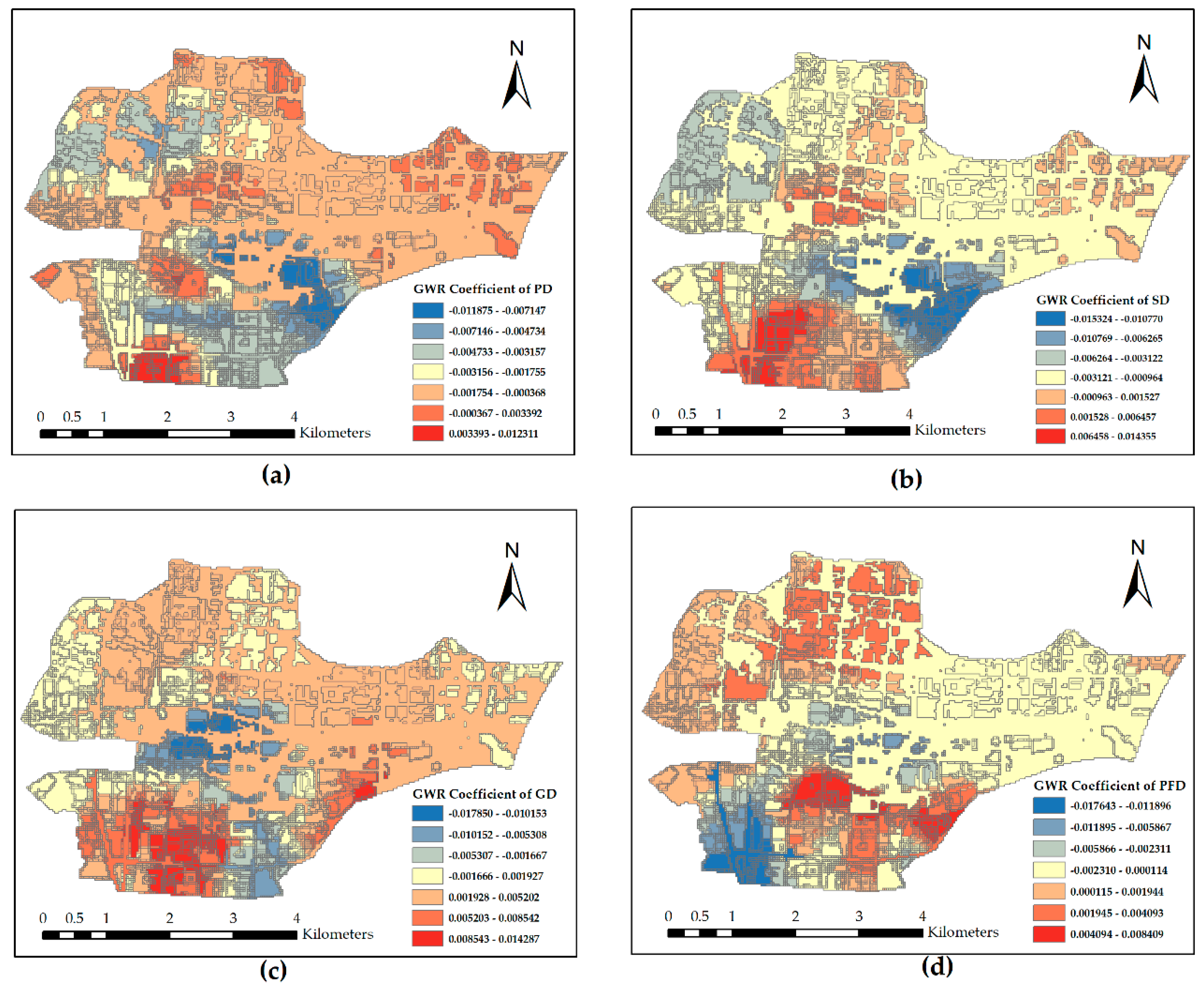
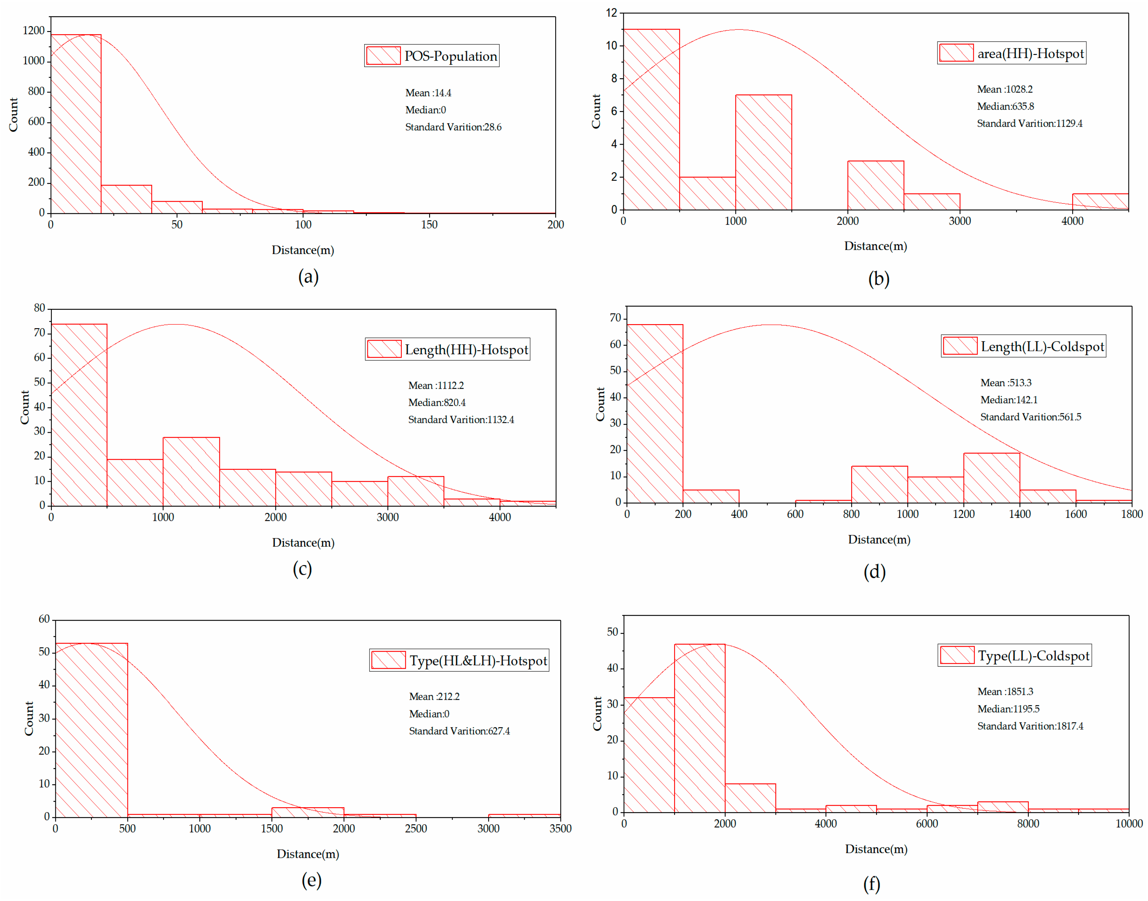
3.3. Correlation Analysis between Population and Public Open Spaces

With the rapid economic and social development, many people are crowding into the city. Considering the fact that urban public open spaces cannot meet the activity needs of the highly dense population, it is of great research value to quantitatively analyze public open spaces with population as an influence factor [33,34]. In this paper, high/low clustering analysis (Getis-Ord General G) was first used to analyze the distribution characteristics of population data in the study area. The results show that the spatial autocorrelation of population distribution is significant, and the spatial clustering is high. Then hot spot analysis was used to further analyze the population distribution characteristics. We superimposed the population hot spot analysis results with the local autocorrelation results of public open spaces area, as shown in Figure 6.
The population of the built-up area is characterized by the spatial sub-bureau with Yuying brook as the boundary. The southern part of the lake is concentrated with high values, which are distributed near public facilities such as parks, squares, and shopping malls in the center of the built area and the south. In the north and west, there are low-value clusters, because the north and west are mainly development zones. In the southwest, there are places that only high-income people can afford, such as villas and mansions. However, in the three street areas outside the built-up area, the low-value clustering feature only appeared in the town center and the vicinity of important traffic lines, and there was no high-value clustering feature distribution. Therefore, the characteristics of population distribution have an obvious correlation with the spatial differentiation of public open spaces. To validate the results of correlation analysis, we calculated the polygons distance between the population cluster area and the aggregation areas of public open spaces, as shown in Figure 7.
We calculated the distance between public open spaces and population by using the neighborhood analysis, and this distance refers to the closest distance of these polygons. The smaller the distance, the closer the polygons are, and the closer the relationship between public open spaces and population. So, we could calculate the histogram of the distance between these polygons to judge their correlation. It should be noted that what is measured here is the relationship between the aggregation of these factors, which means that what we analyzed is the spatial relationship between the local autocorrelation analysis results and hot spot analysis results. According to Figure 7a, we found that distances of these polygons are mostly close to 0, the mean value is just 14.44, which means they are all close to each other. However, we should note that it does not fully indicate that they have a significant correlation, because there are many polygons with no significant aggregation, and there is no distinction between high-value and low-value aggregation areas. Therefore, we need to analyze the correlation between high-value clusters in LISA results of public open spaces and hot spots of population, and the correlation between the low-value clusters and the cold spots. According to Figure 7b–f, we found that the distance between polygons of length (LL) and polygons of cold spot is the shortest, which means that the low-value cluster of the length of public open spaces has a significant correlation with cold spots of population, and the same is true for the high-value cluster of type of public open spaces and hot spots of population.
In conclusion, the experimental results are in line with the actual situation. Taking population as the factor, the spatial distribution characteristics of public spaces are further analyzed from the perspective of the geographic environment and transportation facilities. This shows that the design of public open spaces in the built-up area of Deqing meets the needs of residents. However, the further away from the built-up area, the less space there is for public activities. Combined with the results of SDG 11.7, the per capita public open spaces and the rate of green land in urban built-up areas were 8.63 m2 and 38%, respectively, which are higher than the SDG index, the index value of the dashboard, and the target of the country plan in 2030. However, in other townships, except for built-up areas, the per capita public open spaces are relatively low. The results of the index align with the results of this study and provide a scientific basis for the discovery of problems in the construction of public open spaces in Deqing, in order to further optimize the construction and provide certain technical support and construction guidance and balanced and sustainable economic development between urban and rural areas.

4. Discussion

The results indicate that GIS spatial autocorrelation analysis can help us to describe the different spatial pattern of urban public open spaces, and to identify the causal relationship with population.

4.1. Understanding Global and Local Spatial Pattern of Urban Public Open Spaces

In line with early research by Cybriwsky [35], Johnson [36] and Mitchell [37] that highlighted the importance of understanding spatial pattern and formation mechanism of urban public open spaces in the field of urban planning and urban sustainability evaluation, the findings from this case study demonstrate that the formation of urban public space is positively associated with the urban population. In addition, the results show that global spatial autocorrelations are significant and this kind of autocorrelation has obvious local aggregation characteristics. Different from the research by Fan [17] and Xia [18], which just used local spatial autocorrelation analysis to find the relationship or evaluate the spatial pattern, the current work further found that there are both global and local differentiation characters of spatial pattern for urban public open spaces, and the main factor causing this difference is the population by hot spot analysis. In addition, our results indicate that the local spatial relationships are associated with urban public open spaces. This finding can further verify the spatial justice evaluation of public open spaces, which was also proven by previous studies [38].

4.2. Assessment of Urban Public Open Spaces by SDG 11.7.1

Meanwhile, according to the assessment of SDG11.7, it can be seen that the per capita public open spaces area and green space rate of Deqing’s urban built-up areas in 2016 have reached the goals of the UN 2030 Agenda for Sustainable Development. According to the Section 2.2.4, we calculated these indicators for Deqing and compared the results with the UN 2030 goals. Table 2 shows the calculation and comparison results of Deqing in 2016.
According to the Table 2, the value of most indicators of Deqing in 2016 surpassed one of UN goals in 2030, which means that Deqing already has a high level of sustainable development in terms of urban public open spaces, especially in the built-up area.

4.3. The Relationship between Population Agglomeration and the Types of Public Open Spaces

According to the analysis results in Section 3.3, we have shown that the distribution of public open spaces has a significant relationship with the population, and the relationship represented by different attributes of public open spaces is also different. As shown in Figure 7, high-value cluster of type of public open spaces is related to the high-value cluster of population, and a low-value cluster of length is related to the cold spots. So, the population agglomeration should also have a relationship with the different types of public open spaces, but how does this correlation present? We tried to use the GWR model [39] to analyze this correlation.
Since we are concerned about the relationship between population agglomeration and various types of public open spaces, we have used PD (distance to park), SD (distance to square), GD (distance to green land) and PFD (distance to public facilities) as the influencing factors of population distribution through multicollinearity diagnostic analysis.
Let the number of populations be yi, and the coordinates of the i-th point be (ui,vi), then the GWR model of populations is:
y i = β 0 ( u i , v i ) + j = 1 , k x i , j ( P D ) ( u i , v i ) + j = 1 , k x i , j ( S D ) ( u i , v i ) + j = 1 , k x i , j ( G D ) ( u i , v i ) + j = 1 , k x i , j ( P F D ) ( u i , v i ) + ε i
By calculating the regression coefficient corresponding to each factor, the minimum, upper quantile, median, lower quartile, maximum and average of the regression coefficient of the adjusted spatial kernel were calculated. Then we used the Monte Carlo method to perform a significant test on the spatial variability of each factor, and estimated the p-value of the regression coefficient, as shown in Table 3 and Figure 8.
A comparative analysis of the p-value shows that PFD exhibits significant spatial instability, and their regression coefficients change with spatial location. Most of these coefficients are negative numbers, which means that the concentration of population decreases as the distance to public open spaces increases. Comparing and analyzing the mean of coefficients, it can be seen that the absolute value of the coefficient of PD is the largest, and it has the largest impact on the degree of population aggregation, followed by SD, GD, and PFD. From Figure 8, we can also see that the difference in the distribution of the coefficients of PFD is the most obvious (Figure 8d), while the distribution of the coefficients of PD is more even, and the high values are more concentrated (Figure 8a). Therefore, the park has the most significant correlation with population agglomeration.

5. Conclusions

This paper obtained data of public open spaces in the built-up area and surrounding streets of Deqing based on remote sensing interpretation. Based on the ideas of geographic statistics and spatial analysis, spatial statistical models such as spatial autocorrelation and correlation analysis were used to analyze the spatial distribution characteristics of public open spaces in the built-up area of Deqing in 2016 and its relationship with the population. The area LISA results show that high-value aggregation in public spaces is mainly distributed in the development zone in the west of the built-up area. The clustering of HL is mainly distributed in the center and edge of the built-up area. The edge area shows scattered distribution of low values of public space and has no spatial autocorrelation, but it still influenced the autocorrelation of public open spaces in the built-up area significantly. In addition, different attributes of public open spaces have shown different LISA results—the type has the most positive and significant global autocorrelation, but it also has the worst local aggregation, and the length of public open spaces has the similar local aggregation with the area.
Based on the result of correlation analysis, it is found that the spatial differentiation pattern of public open spaces is significantly related to population agglomeration. The further away from the built-up area, the less public space there is, and lower population agglomeration. The high-value cluster of type of public open spaces is related to the high-value cluster of population, and a low-value cluster of length is related to its cold spots. The results of geographically weighted regression show that different types of public open spaces have different relationships with the population, and the park has the most significant correlation with population agglomeration.
In addition, the assessment results of SDG 11.7.1 indicate that the per capita public open spaces area and green lands rate of Deqing’s built-up areas in 2016 have reached the goals of the UN 2030 Agenda for Sustainable Development. Therefore, it shows that an excellent livable environment and high level of sustainable development in Deqing’s built-up area, but the balance of urban and rural public open spaces needs to be further improved. This study provides a scientific basis for the optimization and construction of public open spaces in Deqing. It also provides experience and a demonstration for other regions in China to carry out quantitative assessment of SDGs, contribute Chinese wisdom to the global implementation of the sustainable development agenda, and propose Chinese solutions.
The results from this study could identify the spatial pattern of urban public open spaces by GIS spatial autocorrelation analysis, but it is worthwhile to state that this kind of spatial pattern difference is very susceptible to policy intervention, especially in cities in China. Although Chinese urban planners now attach great importance to the impact of urban public open spaces, considering the mismatch between urban spaces and socio-economic activities, the autocorrelation of urban public open spaces may change in the future. So, we need more data from different time periods to explore the formation rules
Additionally, the formation mechanism of urban public open spaces is complex and diverse, and it is reliable to analyze the relationship of urban public open spaces with population as the main factor, but if we want to thoroughly understand the formation mechanism of urban public open spaces, we need to analyze more factors, such as public facilities, roads and traffic, government investment, human behavior, and other socio-economic factors. In addition, Deqing is an example of a high degree of urban sustainable development worldwide, so the experimental results of this case are more ideal, but they may not necessarily applicable to other cities with low sustainable development. We need more cases to verify or obtain more general research conclusions. However, limited by data availability, selecting all the cities of different characteristics and development patterns is unachievable. In future studies, more factors may be analyzed based on the current analytical framework, and the proposed method may be applied to other cities to further examine whether the findings of the present study are suitable for various city types.

Author Contributions

Conceptualization, Changfeng Jing and Mingyi Du; Methodology, Qiang Chen; Software, Qianhao Cheng; Validation, Qiang Chen; Formal Analysis, Qiang Chen; Investigation, Qianhao Cheng; Resources, Qiang Chen; Data Curation, Qiang Chen; Writing-Original Draft Preparation, Qiang Chen; Writing-Review & Editing, Mingyi Du; Visualization, Changfeng Jing; Supervision, Mingyi Du; Project Administration, Mingyi Du; Funding Acquisition, Mingyi Du. All authors have read and agreed to the published version of the manuscript.

Funding

This research was funded by National Natural Science Foundation of China (41801235 and 419306500) and National Key Research and Development Program of China (2018YFC0706003).

Acknowledgments

The authors gratefully acknowledge the Geomatics Center of Deqing for providing the original data.

Conflicts of Interest

The authors declare no conflict of interest.

References

  1. Chen, J.; Ren, H.; Geng, W.; Peng, S.; Fanghong, Y.E. Quantitative measurement and monitoring sustainable development goals (SDGs) with geospatial information. Geomat. World 2018, 25, 1–7. [Google Scholar]
  2. Liu, S.; Bai, J.; Chen, J. Measuring SDG 15 at the county scale: Localization and practice of SDGs indicators based on geospatial information. Int. J. Geo Inf. 2019, 8, 515. [Google Scholar] [CrossRef] [Green Version]
  3. Jalaladdini, S.; Oktay, D. Urban public spaces and vitality: A socio-spatial analysis in the streets of cypriot towns. Procedia Soc. Behav. Sci. 2012, 35, 664–674. [Google Scholar] [CrossRef] [Green Version]
  4. Xin, F. Construction of urban community public space under the view of “three governance integration”—Based on the exploration of d community in Shanghai. J. Soc. Sci. 2018, 3, 21–28. [Google Scholar]
  5. Luo, S.; Zhen, F. How to evaluate public space vitality based on mobile phone data:An empirical analysis of Nanjing’s parks. Geogr. Res. 2019, 38, 1594–1608. [Google Scholar]
  6. Pietrzyk-Kaszyńska, A.; Czepkiewicz, M.; Kronenberg, J. Eliciting non-monetary values of formal and informal urban green spaces using public participation GIS. Landsc. Urban Plan. 2017, 160, 85–95. [Google Scholar] [CrossRef]
  7. Xu, L. A review of urban public space research in contemporary China from a sociological perspective. Theory Mod. 2017, 6, 122–128. [Google Scholar]
  8. Yu, L.I.; Zhu, W. An introduction of active design guidelines: Promoting physical activity and health in design of New York city and thinking of urban sapce in Beijing city. World Archit. 2013, 9, 125–128. [Google Scholar]
  9. Nielsen, C.S. The democratic potential of artistic expression in public space: Street art and graffiti as rebellious acts. In Street Art of Resistance; Springer: Berlin/Heidelberg, Germany, 2017; pp. 301–323. [Google Scholar]
  10. Zhang, F.; Xiao, Y.; Yin, W.U. Spatial layout of public sports venues in urban communities—Based on yangpu district of Shanghai. J. Shanghai Univ. Sport 2014, 1, 80–83. [Google Scholar]
  11. Bahrini, F.; Bell, S.; Mokhtarzadeh, S. The relationship between the distribution and use patterns of parks and their spatial accessibility at the city level: A case study from Tehran, Iran. Urban For. Urban Green. 2017, 27. [Google Scholar] [CrossRef] [Green Version]
  12. Alessandro, R.; Matthew, B.; Viniece, J. Inequities in the quality of urban park systems: An environmental justice investigation of cities in the United States. Landsc. Urban Plan. 2018, 178, 156–169. [Google Scholar]
  13. Florindo, A.A.; Barrozo, L.V.; Cabral-Miranda, W.; Rodrigues, E.Q.; Turrell, G.; Goldbaum, M.; Cesar, C.L.G.; Giles-Corti, B. Public open spaces and leisure-time walking in Brazilian adults. Int. J. Environ. Res. Public Health 2017, 14, 553. [Google Scholar] [CrossRef] [PubMed] [Green Version]
  14. Sun, K.; De Coensel, B.; Filipan, K.; Aletta, F.; Van Renterghem, T.; De Pessemier, T.; Joseph, W.; Botteldooren, D. Classification of soundscapes of urban public open spaces. Landsc. Urban Plan. 2019, 189, 139–155. [Google Scholar] [CrossRef] [Green Version]
  15. Shirowzhan, S.; Lim, S.; Trinder, J. Enhanced autocorrelation-based algorithms for filtering airborne lidar data over urban areas. J. Surv. Eng. 2016, 142, 4015008. [Google Scholar] [CrossRef] [Green Version]
  16. Mohammad, A.A.; Reza, S.D.; Abdolreza, R.A.; Mohammadreza, R. Applying GIS to identify the spatial and temporal patterns of road accidents using spatial statistics (case study: Ilam Province, Iran). Transp. Res. Procedia 2017, 25, 2126–2138. [Google Scholar]
  17. Fan, C.; Myint, S. A comparison of spatial autocorrelation indices and landscape metrics in measuring urban landscape fragmentation. Landsc. Urban Plan. 2014, 121, 117–128. [Google Scholar] [CrossRef]
  18. Xia, C.; Anthony, G.-O.Y.; Zhang, A. Analyzing spatial relationships between urban land use intensity and urban vitality at street block level: A case study of five Chinese megacities. Landsc. Urban Plan. 2020, 193, 103669. [Google Scholar] [CrossRef]
  19. Shen, L.; Guo, X. Spatial quantification and pattern analysis of urban sustainability based on a subjectively weighted indicator model: A case study in the city of Saskatoon, SK, Canada. Appl. Geogr. 2014, 53, 117–127. [Google Scholar] [CrossRef]
  20. Majumdar, D.D.; Biswas, A. Quantifying land surface temperature change from LISA clusters: An alternative approach to identifying urban land use transformation. Landsc. Urban Plan. 2016, 153, 51–65. [Google Scholar] [CrossRef]
  21. Ginebreda, A.; Sabater-Liesa, L.; Rico, A.; Focks, A.; Barceló, D. Reconciling monitoring and modeling: An appraisal of river monitoring networks based on a spatial autocorrelation approach—emerging pollutants in the Danube River as a case study. Sci. Total Environ. 2018, 618, 323–335. [Google Scholar] [CrossRef]
  22. Ren, H.; Shang, Y.; Zhang, S. Measuring the spatiotemporal variations of vegetation net primary productivity in Inner Mongolia using spatial autocorrelation. Ecol. Indic. 2020, 112, 106108. [Google Scholar] [CrossRef]
  23. Li, R.; Chen, N.; Zhang, X.; Zeng, L.; Wang, X.; Tang, S.; Li, D.; Niyogi, D. Quantitative analysis of agricultural drought propagation process in the Yangtze River Basin by using cross wavelet analysis and spatial autocorrelation. Agric. For. Meteorol. 2020, 280, 107809. [Google Scholar] [CrossRef]
  24. Tan, L.Y.; Li, Q.; Tan, L. Spatial statistics analysis of RJGDP fo Beijing Tianjin and Hebei based on R. J. North China Inst. Sci. Technol. 2015, 3, 105–110. [Google Scholar]
  25. Wang, W.; Chang, Y.; Wang, H. An application of the spatial autocorrelation method on the change of real estate prices in Taitung City. ISPRS Int. J. Geo Inf. 2019, 8, 249. [Google Scholar] [CrossRef] [Green Version]
  26. Blazquez, C.A.; Picarte, B.; Calderón, J.F.; Losada, F. Spatial autocorrelation analysis of cargo trucks on highway crashes in Chile. Accid. Anal. Prev. 2018, 120, 195–210. [Google Scholar] [CrossRef] [PubMed]
  27. Chen, Y. New approaches for calculating Moran’s index of spatial autocorrelation. PLoS ONE 2013, 8, e68336. [Google Scholar] [CrossRef] [Green Version]
  28. Waldhör, T. The spatial autocorrelation coefficient Moran’s I under heteroscedasticity. Stat. Med. 1996, 15, 887–892. [Google Scholar] [CrossRef]
  29. Anselin, L. Local indicators of spatial association—LISA. Geogr. Anal. 1995, 27, 93–115. [Google Scholar] [CrossRef]
  30. Kondo, K. Hot and cold spot analysis using Stata. Stata J. 2016, 16, 613–631. [Google Scholar] [CrossRef] [Green Version]
  31. Prasannakumar, V.; Vijith, H.; Charutha, R.; Geetha, N. Spatio-temporal clustering of road accidents: GIS based analysis and assessment. Procedia Soc. Behav. Sci. 2011, 21, 317–325. [Google Scholar] [CrossRef] [Green Version]
  32. Wheeler, D.C.; Páez, A. Geographically weighted regression. In Handbook of Applied Spatial Analysis; Springer: Berlin/Heidelberg, Germany, 2010; pp. 461–486. [Google Scholar]
  33. Dong, N.; Yang, X.; Huang, D.; Han, D. Spatialization method of demographic data based on urban public facility elements. J. Geo Inf. Sci. 2018, 20, 918–928. [Google Scholar]
  34. Gao, J.; Fu, J.; Ye, C. Spatial characteristics and causes of urban public service facilities in Guangzhou city. Areal Res. Dev. 2012, 31, 71–75. [Google Scholar]
  35. Cybriwsky, R. Changing patterns of urban public space: Observations and assessments from the Tokyo and New York metropolitan areas. Cities 1999, 16, 223–231. [Google Scholar] [CrossRef]
  36. Johnson, A.J.; Glover, T.D. Understanding urban public space in a leisure context. Leis. Sci. 2013, 35, 190–197. [Google Scholar] [CrossRef]
  37. Mitchell, D. Introduction: Public space and the city. Urban Geogr. 1996, 17, 127–131. [Google Scholar] [CrossRef]
  38. Izzy, Y.J.; Luo, J.; Chan, E.H.W. Spatial justice in public open space planning: Accessibility and inclusivity. Habitat Int. 2020, 97, 102–122. [Google Scholar]
  39. Brunsdon, C.; Fotheringham, A.S.; Charlton, M. Some notes on parametric significance tests for geographically weighted regression. J. Reg. Sci. 1999, 39, 497–524. [Google Scholar] [CrossRef]
Figure 1. Built-up areas and geographic location of Deqing County.
Ijgi 09 00575 g001
Figure 2. Remote sensing image of built-up area (true color synthesis, 2017-3-11).
Ijgi 09 00575 g002
Figure 3. Spatial distribution of population in Deqing County.
Ijgi 09 00575 g003
Figure 4. Global autocorrelation analysis results of public open spaces in terms of area: (a) whole area; (b) built-up area.
Ijgi 09 00575 g004
Figure 5. Local autocorrelation analysis results of public open spaces on: (a) area in whole area, (b) area in built-up area, (c) length in whole area, (d) length in built-up area, (e) type in whole area, (f) type in built-up area.
Ijgi 09 00575 g005
Figure 6. Hot spot analysis results of population and overlaid results with the local indicators of spatial association (LISA) of public open spaces area.
Ijgi 09 00575 g006
Figure 7. Statistic results of polygons distance between: (a) public open spaces and population; (b) area (HH) and hot spot; (c) length (HH) and hot spot; (d) length (LL) and cold spot; (e) type (HL and LH) and hot spot; (f) type (LL) and cold spot. * POS: Public Open Spaces.
Ijgi 09 00575 g007
Figure 8. GWR coefficient distribution of four types distances. (a) GWR coefficient of distance to park, (PD); (b) GWR coefficient of distance to square (SD); (c) GWR coefficient of distance to green land (GD); (d) GWR coefficient of distance to public facilities (PFD).
Ijgi 09 00575 g008
Table 1. Statistic results of spatial global autocorrelation analysis.
AttributesArea RangeSpatial Autocorrelation Analysis
Global Moran’IZ-Scorep-Value
AreaWhole area0.0011491.7230.085
Built-up area0.0055782.3530.018
LengthWhole area0.0333213.050.0021
Built-up area0.0464717.1170.0027
TypeWhole area0.1344849.090.0000
Built-up area0.151550.120.0000
Table 2. The assessment results of urban public open spaces by SDG 11.7.1 in Deqing’s built-up area.
IndicatorsDeqing in 2016UN Goals in 2030
Population440,000/
Built-up area (km2)34.64/
Area of public open spaces per capita (m2)8.63>1.5
Proportion of total public open spaces (%)16.515
Ratio of green lands (%)3838.9
Area of green lands per capita(m2)15.314.6
Table 3. The statists of regression coefficient and p value in geographically weighted regression (GWR) model.
FactorsMinimumUpper QuartileMedianLower QuartileMaximumMeanp-Value
Intercept1.4034256.6713958.5931210.9068515.178958.4650960.3656
PD−0.01187−0.00398−0.00207−0.000880.012311−0.002310.5132
SD−0.01532−0.00384−0.001730.0004580.014355−0.002050.2006
GD−0.01785−0.001220.001050.0048850.0142870.0011620.3245
PFD−0.01764−0.001540.0004830.0018780.008409−0.000420.0115

