Urban Population Distribution Mapping with Multisource Geospatial Data Based on Zonal Strategy


1
School of Geography and Remote Sensing, Guangzhou University, Guangzhou 510006, China
2
Institute of Land Resources and Coastal Zone, Guangzhou University, Guangzhou 510006, China
*
Author to whom correspondence should be addressed.
ISPRS Int. J. Geo-Inf. 2020, 9(11), 654; https://0-doi-org.brum.beds.ac.uk/10.3390/ijgi9110654
Submission received: 26 September 2020
/
Revised: 24 October 2020
/
Accepted: 28 October 2020
/
Published: 30 October 2020
(This article belongs to the Special Issue Measuring, Mapping, Modeling, and Visualization of Cities)
Abstract
:Mapping population distribution at fine resolutions with high accuracy is crucial to urban planning and management. This paper takes Guangzhou city as the study area, illustrates the gridded population distribution map by using machine learning methods based on zoning strategy with multisource geospatial data such as night light remote sensing data, point of interest data, land use data, and so on. The street-level accuracy evaluation results show that the proposed approach achieved good overall accuracy, with determinant coefficient (R2) being 0.713 and root mean square error (RMSE) being 5512.9. Meanwhile, the goodness of fit for single linear regression (LR) model and random forest (RF) regression model are 0.0039 and 0.605, respectively. For dense area, the accuracy of the random forest model is better than the linear regression model, while for sparse area, the accuracy of the linear regression model is better than the random forest model. The results indicated that the proposed method has great potential in fine-scale population mapping. Therefore, it is advised that the zonal modeling strategy should be the primary choice for solving regional differences in the population distribution mapping research.
1. Introduction
People are the main body of geographical environment and social activities, and their distribution pattern is an important subject in many research fields such as sociology, geography, environmental studies, and so on [1,2]. Common population data mainly include two forms: demographic data and spatialized data. Currently, using demographic data based on administrative units is the main way to obtain population distribution information. Although the census data have the advantages of being comprehensive, accurate, and authoritative [3,4], they have the disadvantages of low spatial resolution, excessively long statistical period, and low update frequency. Therefore, the low spatial and temporal resolution of census data is not conducive to effective urban governance. Compared with demographic data, spatialized population data can express the true population distribution more intuitively and on multiple scales, thereby effectively overcome the shortcomings of demographic data.
In recent years, the emergence of multi-source data such as point of interest (POI for short), location check-in data, sharing-bikes’ trajectories, floating car GPS, and night light remote sensing data provide time-efficient, fine-grained, and reliable data source for gridded population distribution estimation, while machine learning technologies provide advanced methods for simulating gridded population distribution. Hence, with the progress of data sources and research methods, it is possible to accurately understand the urban population distribution in multiple scales and recognize spatiotemporal patterns [5,6,7]. Guangzhou is one of the core cities of Guangdong-Hong Kong-Macao Greater Bay Area. Due to the fast urbanization process, it is facing several threats, such as large population, high population density, traffic congestion, and irrational allocation of resources. To solve the above problems, detailed population distribution information is essential basic information.
Research on the population distribution map can be traced back to 1930. American social geographer Wright J.K. proposed the dasymetric method, which combined population distribution with land use types to generate a population distribution map of Cape Cod, Massachusetts [8]. Based on the literature review, approaches used to map populations differ in techniques (disaggregation or aggregation), mapping unit (e.g., administrative units, enumeration units, geographical units, regular grid), ancillary data used (e.g., topographic maps, land use/land cover vector data-sets, cadastral data, satellite images, LIDAR data, etc.), and visualization methods (e.g., choropleth map, isolines, dasymetric map, 3D visualization) [9]. In this paper, we focus on the disaggregation mapping technique in grid unit. Regarding the gridded population distribution data research, existing studies can be divided into different scales such as global, country, city, and commune. In the 1990s, many global population datasets were developed, such as the Gridded Population of the World (GPW), the Gridded Rural Urban Mapping Project (GRUMP), LandScan, Worldpop, and so on. These global population datasets employed different ancillary datasets with various approaches. In spite of these, datasets are important for the data-poor regions; their accuracies in city or commune scale are still worth noting. The authors developed an automatic and powerful method to improve the mapping accuracy of GPW dataset, by detecting and mitigating major discrepancies and anomalies occurring in geospatial census data [10]. Their work illustrates the value and possible contribution of detailed, updated, and independent remote sensing data to complement and improve conventional sources of fundamental population statistics. In their work, global and consistent remote sensing-derived data reporting on built-up presence was used to revise census units deemed as ‘unpopulated’ and to harmonize population distribution along coastlines. The results show that the targeted anomalies were significantly mitigated and that the baseline census database has improved, potentially benefitting other uses of the same statistical base. There are also some scholars who tried to conduct high-resolution population research at the national level [11,12,13]. However, there are relatively few detailed studies on small-scale areas such as cities, due to the various urban fabric patterns and city complexity. As the basic unit of China’s economic activities and social management, cities urgently need precise and accurate population distribution information to improve the level of urban governance.
In summary, gridded population distribution is usually simulated in four different ways, including spatial interpolation method, land use inversion method, night lighting modeling method, and multi-source data fusion method. Each method has its advantages and drawbacks. The spatial interpolation method uses interpolation algorithm to obtain gridded population distribution data by taking census data as model input [14,15,16] and has been widely applied for the spatial decomposition of census data [17,18,19]. The gridded population data can be interpolated directly, or based on the information provided by other auxiliary data, thus it is divided into regional interpolation without auxiliary data and regional interpolation with auxiliary data. Commonly used spatial interpolation methods include point interpolation and area weight interpolation. The implementation steps of the point interpolation method are as follows. First, control points in the study area are selected and the density of the center point are used to symbolize the population density of each source area. Then, an appropriate interpolation algorithm (such as Inverse distance weighted (IDW), Kriging, etc.) is selected to generate population density raster map. Finally, the gridded population map is obtained by overlaying population density raster map and the administrative boundary. This method is relatively easy to implement, but it has severe limitations. First, the spatial resolution of model outputs is generally coarse, mostly at tens of kilometers. Second, the model’s error is difficult to quantify. Third, regional interpolation is affected by the error of the original region aggregation or decomposition operation, and its accuracy largely depends on how to define the original region and the target region, the degree of generalization during the interpolation process, and the characteristics of the partition surface [20]. Therefore, the ability of spatial interpolation method to describe the real population distribution is weak.
The principle of land use inversion method is to give different weights to each land use type according to the differences of population density between different land use types [18,21,22,23]. However, the land use inversion method fails to reflect the population distribution difference in the same type of land parcels, and ignores the randomness of population distribution. Since the launch of the DMSP/OLS satellite in 1970s, the night light modeling method has become one of the mainstream methods for simulation of gridded population distribution [24,25,26]. However, the application of DMSP/OLS data is relatively rare, because the sensor stopped working in 2013 and the spatial resolution is too low(1KM). The emergence of Suomi National Polar-Orbiting Partnership Visible Infrared Imaging Radiometer Suite (NPP-VIIRS) data effectively overcomes the shortcomings of DMSP-OLS data in spatio-temporal resolution [27], and such data are more suitable for the study of human social and economic activities [28,29]. Sutton K. et al. used DMSP/OLS night light data to estimate the global population based on a global scale, and found that the global population is about 6.3 billion [30]. However, spatial resolution of DMSP/OLS and NPP/VIIRS night light data sources are still to coarse for population modelling in local scale. Nowadays, the world’s first professional luminous remote sensing satellite designed by Wuhan University (Wuhan, China), Luojia 1-01 (LJ 1-01), was successfully launched in June 2018. Compared to NPP-VIIRS data, LJ 1-01 data have a significant improvement in spatial resolution and quantitative level, which provide a more refined data source for small-scale population distribution simulations [31,32,33]. In essence, the night light modeling method simulates the gridded population distribution in the study area by establishing a linear relationship between the night light intensity and population density. However, the problems in the night light data seriously affect the accuracy of the model outputs, such as pixel saturation, overflow, and low accuracy of population retrieval in weak light areas. In order to improve the simulation accuracy, some scholars have tried to combine night lighting data with land use data for research [34,35,36]. However, the improvement in accuracy was not significant. Then, some scholars attempted to improve the simulation accuracy by combining the night lights data, land use data, Point of interest (POI) data, and other types of data [37,38,39]. With the continuous enrichment of social sensing data, some scholars attempt to depict the dynamics of population distribution by using these data, such as taxi GPS data [40], mobile phone data [41], tencent location service data [42], baidu heat map data [43], and so on. The multi-source data fusion method has become one of the most popular method. Due to the limitations of these data, including poor data availability, data heterogeneity, and so on, the conditions for producing gridded population distribution dataset at a large-scale are not yet mature.
Essentially, the spatial decomposition of census data to grid unit is a regression process. Several regression models have been proposed to create the weight layer, such as linear regression (LR), geographically weighted regression (GWR), random forest regression, and so on [23,44]. In particular, the random forest (RF for short), one machine learning method which was first systematically proposed by Breiman [45], is becoming more and more popular in the study of models to produce the weighting layer of population data, as it has several advantages including suitable for collinearity, avoiding over-fitting, high calculation speed, and so on. The idea of RF algorithm is to use the bootstrap resampling method to extract multiple samples from the original sample, model the decision tree for each bootstrap sample, and then combine the results of multiple decision trees to obtain the final regression result by voting. For the first time, scholars obtained 100 m grid population mapping results in three undeveloped countries [46]. Due to the ease of training and interpretation, the random forest method has received increasing attention in the population mapping research [42,47,48]. In the process of random forest modeling, it is necessary to optimize several parameters for improving the performance and effect of learning, such as the max number of features and the max depth of trees, and so on [49,50]. In general, to avoid the impact of the initial data partition on the results, cross validation (CV) and grid search were usually performed to reduce the occasionality and ensure the validity and accuracy of the model training [51].
The uncertainty of modeling is also an important issue in the study of population distribution mapping, which includes ecological fallacy, modifiable areal unit problem (MAUP), and so on. The MAUP is a classic problem in the Geographical Information Sciences, which has been long acknowledged and explored. For any spatial resolution, as any set of boundaries, MAUP may seriously hamper the strength of statistical results [52]. Sensitivity Analysis is a useful method to explore the uncertainty of modelling. The authors tested the effect of different geometrical data aggregation schemas—administrative regions and hexagonal surface tessellation—on global spatial autocorrelation statistics, by using several datasets for two study-areas including Continental Portugal (mixed urban-rural) and the Lisbon municipality (urban), and raised an important point, i.e., inferences based on spatial analysis of areal data depend greatly on the method used to quantify the degree of proximity between spatial units [52].
As we know, the relationship between population distribution and influencing factors is an extremely complex nonlinear relationship. A variety of machine learning algorithms, including random forests, neural network, and so on, can handle nonlinear relationship fitting well, while a geographic detector model can handle the spatial heterogeneity of influencing factors. However, most existing studies use a single model to the whole area. For regions with large population density differences, a single or global model cannot accurately explain the mechanism of the spatial distribution of internal population. The zonal strategy can effectively solve the shortcomings of the single model, because it can perform secondary partition modeling on the study area according to the characteristics. To this end, this article intends to illustrated the population map of Guangzhou city based on the idea of zoning modeling and machine learning methods, by using multi-source spatial data such as land use, POI, night lights, and so on. This article attempts to improve the study of mapping population distribution, and provide important basic information for urban management.
2. Materials and Methods
In this section, the study area and data source are first introduced (see Section 2.1 and Section 2.2). Second, we needed to select the appropriate grid cell size to rasterize the initial influence factor data based on various calculation formulas (see Section 2.3.1). Third, we identified main factors affecting population distribution based on a geographic detector model (see Section 2.3.2). Finally, we simulated gridded population distribution information of study area based on machine learning algorithms and zonal strategy (see Section 2.3.3 and Section 2.3.4). Moreover, we further evaluated the model accuracy by using several metrics.
2.1. Study Area
Guangzhou, the capital of Guangdong province, lies between 112°57′ E to 114°3′ E longitude and 22°26′ N to 23°56′ N latitude, and has an area about 7434 km2. The study case was conducted in six central urban districts of Guangzhou city, including Yuexiu, Liwan, Tianhe, Haizhu, Huangpu, and Baiyun. In order to ensure consistency with the caliber of population statistics in 2013, the Huangpu district does not contain the street-level units of former Luogang district. These districts have the highest population densities in Guangzhou city and serve as the political, cultural, and economic centers of Guangzhou. According to the data provided by Guangzhou statistics bureau, the resident population of Guangzhou was 15.3059 million in 2019 and the population density of the city was close to 2059 person/km2. However, the study area covers approximately 20.9% of the total area of Guangzhou city, and the recorded permanent resident population comprising 63.18% of the total resident population of Guangzhou. The street-scale population density map of the study area in 2013 is shown in Figure 1.
2.2. Data and Preprocessing
The research data used in the article is shown in Table 1.
The spatial resolution of digital elevation model (DEM) data is 30 m, and the spatial reference is GCS_WGS_1984. The land use data include six major categories of cultivated land, forest land, grassland, water area, urban and rural, industrial and mining, residential land, and unused land, with a spatial resolution of 30 m. With consideration of the proportions and potential for contribution to population distribution, the urban construction and rural housing land use type was reclassified into three subtypes including urban Land, rural land, and the other construction land. Road data includes highways, national highways, provincial highways, urban roads, and county highways. There are thirteen types of POI data, including catering facilities, public facilities, companies and enterprises, shopping facilities, transportation facilities, finance and insurance, scientific, educational and cultural facilities, commercial housing, life service facilities, sports and leisure facilities, medical service facilities, government agencies and social groups, and accommodation facilities. After obtaining the POI data, it is necessary to perform data cleaning work such as deduplication and correction before it can be used normally. At last, all datasets were unified to the Albers project coordinate system. The reference ellipsoid is Krasovsky_1940 ellipsoid.
2.3. Methods
2.3.1. Rasterization of Initial Influence Factor Data
Grid cell size has an important influence on the quality of the population distribution simulation results. The gridded population data with appropriate cell size can reveal the spatial varieties of population distribution pattern more clearly. According to a previous research [53], the most appropriate grid size is almost 10% of the smallest street’s area. ShaMian street is the smallest one in our study case, and its area is 30,8348 square meters. Therefore, the cell size was set to 150 m in our study case. The initial impact factor datasets are rasterized into 150 m. The calculation methods of each factor in grid scale are shown in Table 2.
2.3.2. Identification of Main Factors Based on Geographic Detector Model
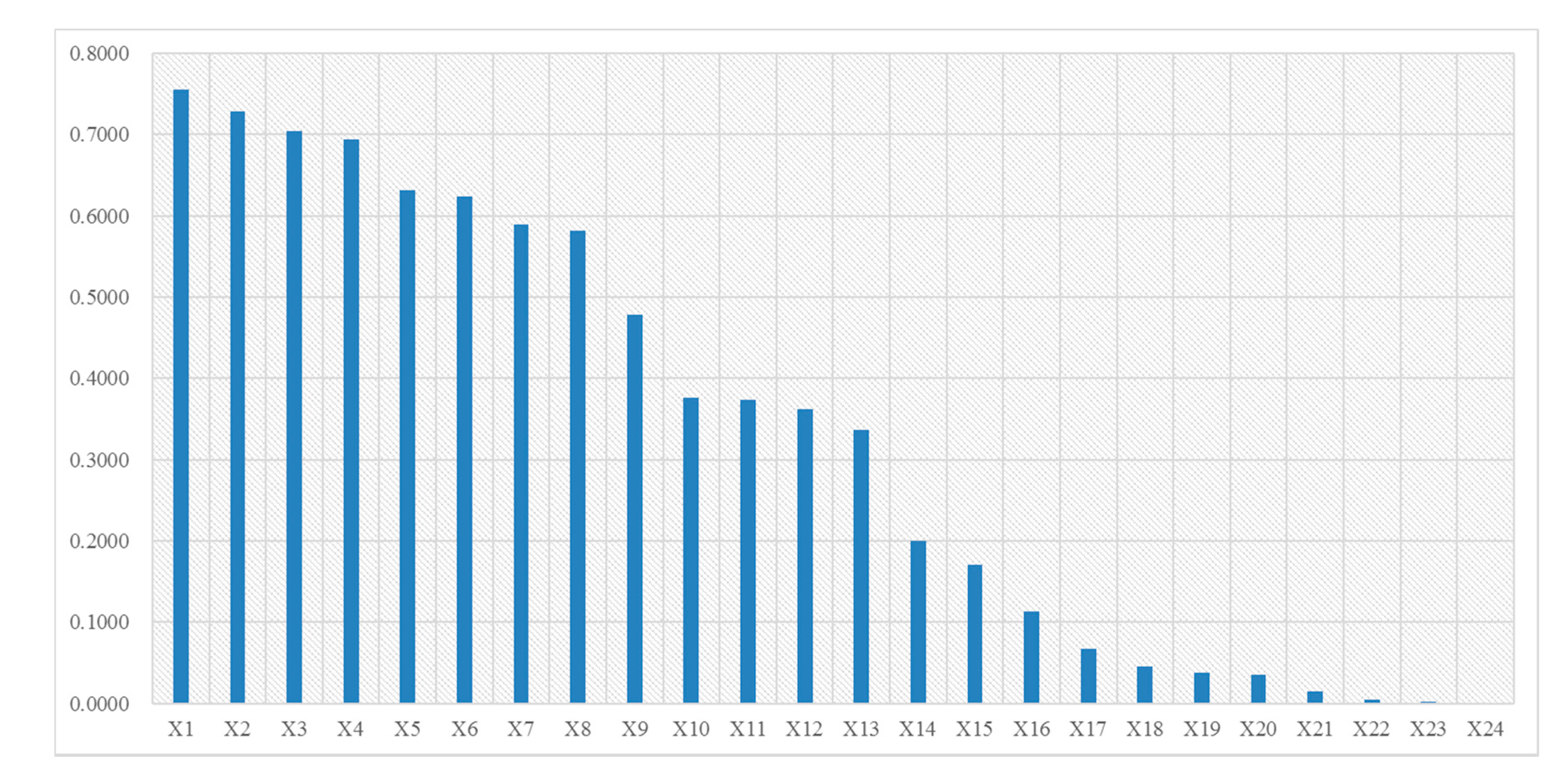
The geographic detector was developed by Wang Jinfeng et al. [54]. It is a statistical method for detecting spatial differentiation and revealing the driving factors behind it. Because this method does not require linear assumptions, and has an elegant form and clear physical meaning, it is widely used in the study of the influence mechanism of social economic, natural environment factors. The geographic detector mainly includes four sub-detectors: factor detector, interactive detection, risk detector, and ecological detector. This paper mainly uses the factor detector to calculate the explanatory power of the influence factor on the population distribution, which is denoted as q value to measure. The q value ranges from 0 to 1. The larger the q value, the stronger the explanatory power of the factor. The initial influence factors (X) include X1 (Government agencies and social organizations), X2 (Public utilities), X3 (Business residence), X4 (Medical service facilities), X5 (Financial insurance facilities), X6 (Transportation facilities), X7 (Science, education and cultural facilities), X8 (Sports and leisure facilities), X9 (Living service facilities), X10 (Catering facilities), X11 (Companies), X12 (Accommodation service facilities), X13 (Shopping facilities), X14 (Night light intensity), X15 (Index of urban land use), X16 (Altitude), X17 (Building area), X18 (Index of arable land), X19 (Index of wood land), X20 (Road network density), X21 (Index of rural land), X22 (Index of other construction land), X23 (Index of waters), and X24 (Index of grass land).
First, the Create Random Points tool in ArcGIS 10.2 (ESRI Inc., Redland, USA) was used to randomly generate 3000 sample points in the study area. Then, the extract multi values to Points tool was used to extract the population density values of the corresponding sample points and the index values of each factor. Finally, the GeoDetector2015 software (Wang Jinfeng et al. [54], Beijing, China) was used to calculate the explanatory power (q value) of the influence factor (X) for the population density (Y).
The analysis results of the geographic detector model are shown in Figure 2. The results show that, except for the water area index and grassland index, the significance level of remain factors is 0.05. In other words, except for the water area index and grassland index, remain factors have obvious impact on population density. From the explanatory power ranking results, socioeconomic factors have a greater impact on the spatial distribution of population in the study area than natural factors. Among socio-economic factors, except for building area and road network density, the explanatory power values of other impact factors are all above 0.1, indicating a significant impact on the population density. Among the natural factors, except for the urban land use index, the explanatory power q of other influencing factors is relatively small. To improve the model accuracy, five factors including grassland index, water area index, urban land index, rural land index, and other construction land indexes are removed. The final impact factors of population distribution include 20 indicators including cultivated land index, forest land index, night light intensity, elevation, POI impact intensity index, building area, road index, and so on.
The sample features are presented numerically, and the numerical ranges between some different features are quite different. In addition, the dimensions of different features are inconsistent. In order to eliminate the influence of non-uniform dimension and extreme value, the data are normalized. There are 106 records in the street sample dataset after min–max normalization, and each record includes 20 feature values. The grid sample dataset has a total of 48,648 records, and each record contains 20 feature values.
2.3.3. Simulation of Gridded Population Distribution with Single Modeling Strategy
Linear Regression Model
The linear regression model based on land use data and night light remote sensing data is currently a widely used method of spatialization of population data. For this reason, based on NPP/VIIRS night light data and land use data, this paper establishes a linear regression model of the population distribution grid in the study area to realize the spatialization of population data.
The model is built as follows:
where denotes the population data of the i-th street (town); represents the initial coefficient of population distribution for the j-th land use type; represents the j-th land use type index of the i-th street (town); represents the type of land use selected; represents the coefficient of night light intensity; represents the average night light intensity value of each street; and is the constant term.
Random Forest Regression Model
In this research, the street scale data set is used as the training set, and the grid scale data set is used as the development set. The machine learning library used for modeling is scikit-learn 0.21.3, which is a suit of free software released and maintained by scikit-learn international community. First, the model is training using the algorithms selected in the article, taking the population density of each street as the dependent variable, and the influence factors identified by the geographic detector model as the independent variable. During the training process, the best model parameters such as the maximum depth and features of the decision tree were obtained by GridSearchCV function in the scikit-learn which is conducted to try every possibility through loop traversal in all candidate parameter selections. To improve the predictive accuracy and control overfitting [55,56], K-fold cross validation (CV) was used to obtain model parameters. Therefore, 10-fold CV was performed, and the determinant coefficient (R2) score was used to determine the overall accuracy of the model. Then, the optimal model is applied to the grid scale dataset to predict the population density value of each grid cell. Next, the population density is multiplied by the cell area to obtain the population of each cell, and the populations of each cell are merged into the street administrative unit. Finally, the accuracy of model result is evaluated through error indicators such as mean relative error (MRE), root mean square error (RMSE), R2 and so on, taking the demographic data of each street as the true value.
2.3.4. Simulation of Gridded Population Distribution with Zonal Modeling Strategy
Using the population concentration division method, the study area is subdivided to improve the simulation accuracy. The calculation method of population concentration is shown in Equation (2):
where represents the population concentration degree of a certain street (town); and represents the population of the street (town) and the total population of the area respectively; and and represent the area of the street (town) and the total area of the area.
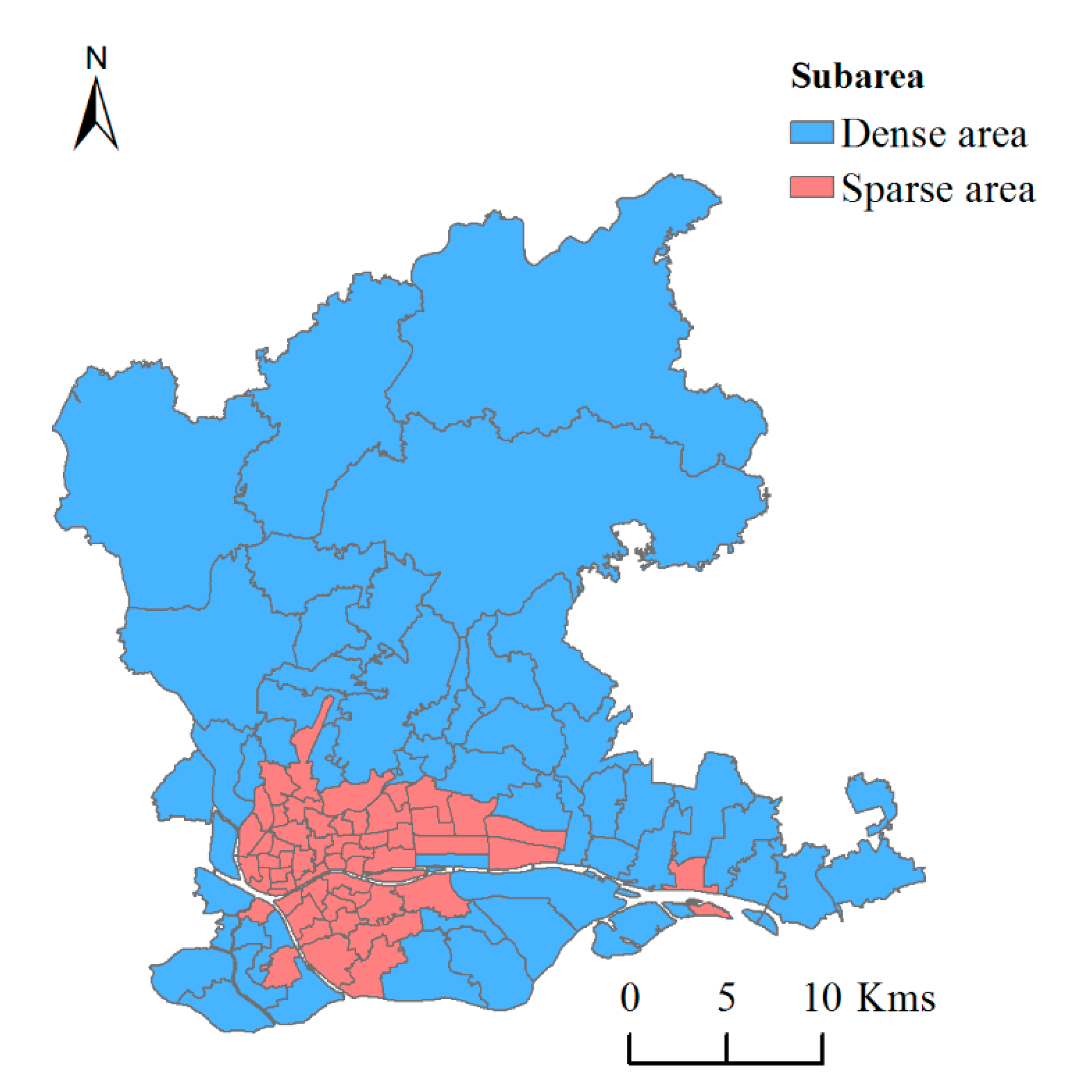
The study area is divided to two partitions according to the classification criteria of population concentration. In order to ensure that each region has a sufficient sample size for machine learning modeling, referring to the Chinese population agglomeration classification standard [57], the study area is divided into two subareas: dense area and sparse area. The dense area contains 54 streets and the average population density is 37,647 people/km2. The non-populated area contains 52 streets and the average population density is 3594 people/km2. The specific zoning results are as follows as shown in Figure 3.
Different model factors were selected for two subareas. For dense area and sparse area, linear regression model and random forest model are both executed. Models suitable for each subarea are selected according to the simulation accuracy and merged to population distribution map for the entire study area.
3. Results
3.1. Simulation Results Based on Global Linear Regression Model
The population density of each street (town) in the study area was taken as the dependent variable, while the urban land index (X1), arable land index (X2), forest land index (X3), rural land index (X4), other construction land index (X5), grassland index(X6), and the average night light intensity (X7) were selected as the independent variables. The model is calculated through linear regression analysis, and is shown in Equation (3):
The value of coefficient of determination (R2) is 0.59, which means that the population density in one street unit is explained in 59% by the land use indices and night light intensity index. The variance analysis results of model are shown in Table 3.
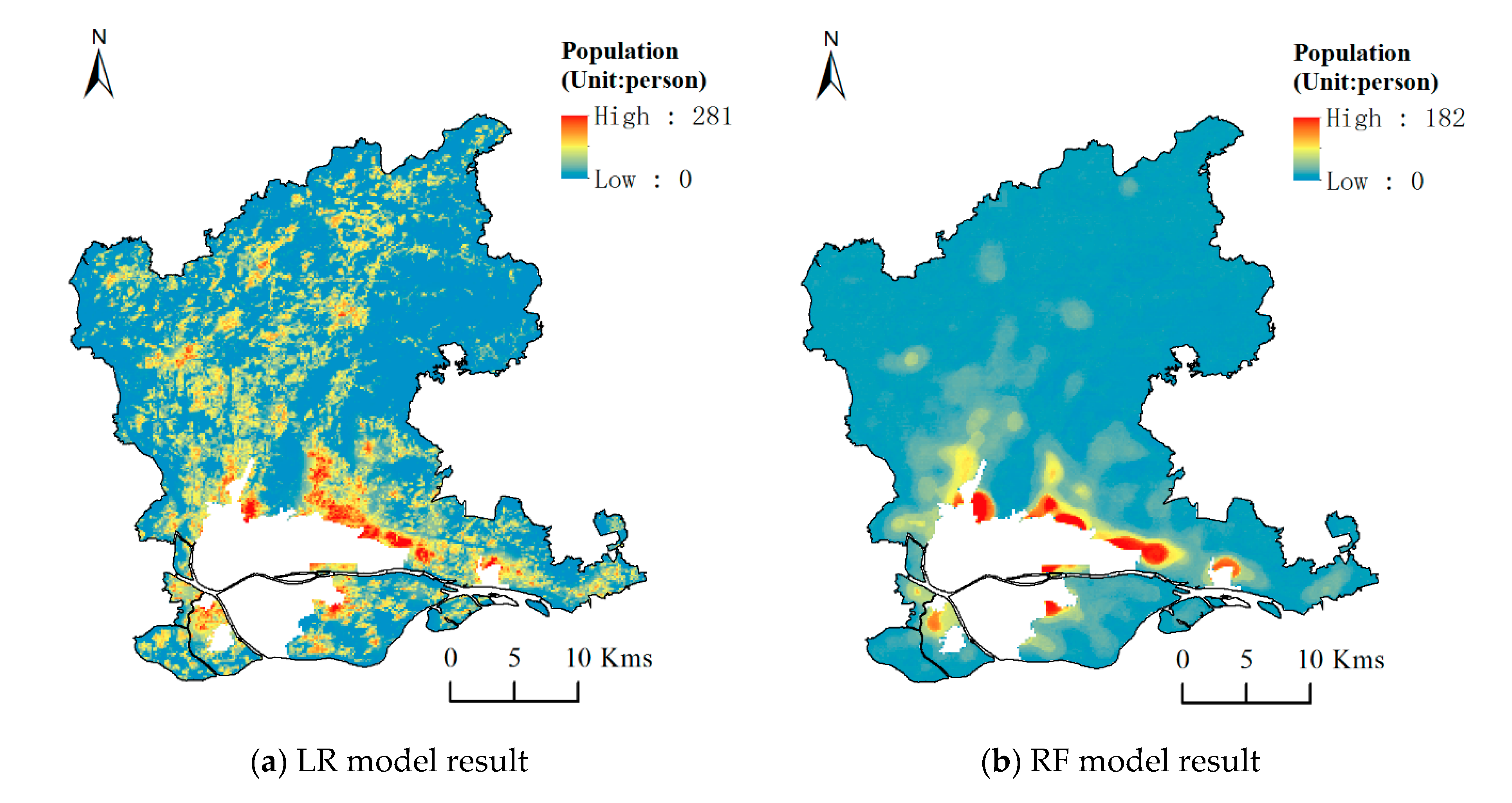
Based on the multiple linear regression Equation (3), the grid calculator in ARCGIS software is used to generate the population distribution data of the study area. The result is shown in Figure 4.
It can be seen from Figure 4 that the population is gradually decreasing from the center of the city to the surrounding area. Because the simulation results are too much affected by the spatial pattern of construction land and the intensity of night lights, the population of the construction land area is overestimated, and the spatial differentiation of population distribution is not obvious. In particular, the northern part of Renhe town is close to Guangzhou Baiyun International Airport (Guangzhou, China) and the industrial area is concentrated, resulting in obvious outliers in population estimates, which are inconsistent with the actual situation. In order to verify the accuracy of the simulation results, a linear fit was performed between the simulated population of the street (town) and the census data. It was found that the goodness of fit (R2) is only 0.0039, and the RMSE is 1,007,871.35. The simulation results in most of the street (town) had a huge deviation from the true value. In a word, the simulation accuracy is very poor. Through comparison of previous studies and analysis, it is found that the reasons for the large deviation of the model estimation may be roughly as follows:
- (1)
- The research area is the downtown area of Guangzhou city, where the factors affecting population distribution in the area are very complicated. It is impossible to accurately simulate the characteristics of population distribution only by relying on land use and night light data.
- (2)
- The spatial resolution of land use data is low, which is only 30 m. At the same time, the resolution of land use types in this study is not detailed enough, which has only five categories. Since the study area is the central urban area of Guangzhou city, the construction land is the dominant land use type in the area. Therefore, in the process of gridded population distribution mapping, simulation result is deeply affected by the spatial distribution pattern and area of the construction land, which easily leads to overestimation and large deviations from actual census data. As we known, previous studies also demonstrate that the higher the resolution of land use data and the more detailed land use types can improve the accuracy of population simulation.
- (3)
- The time of night light data, land use data, and statistical population data are inconsistent. The population census data used in this study case are from 2013, while the land use data and the night light data are from 2015 and from 2016, respectively. The inconsistency between the modeled data and the real data will inevitably lead to a decrease in model accuracy.
3.2. Simulation Results Based on Global Random Forest Model
In order to reduce the simulation error and improve the simulation accuracy, the selection of the factors affecting the spatial distribution of the population is optimized, and the random forest model is adopted to realize the spatialization of population data in the study area. Considering the error factors of the global linear regression model, the independent variables of random forest model were updated to 20 indicators including cultivated land index and woodland index, night light intensity, altitude, POI influence intensity, building area, road network density, and average house prices. Based on the street (town) scale, the training feature database was built. Due to the inconsistent dimensions of the influencing factors, the data was standardized to eliminate the influence of inconsistent dimensions and extreme values.
As the number of streets being used to fit the model is only 106, 10-fold CV was chosen. It means that 9-fold samples were adopted into the model to obtain the proper parameters and the accuracy was assessed using the remaining samples. The 10-fold cross validation and grid search were conducted to find the proper parameters in the RF model (Table 4). When the max depth of the decision tree was 9 and the number of estimators was 500, the determinant coefficient (R2) of the CV score reached the maximum value of 0.7250. Finally, we built a random forest model by setting the maximum depth of subtrees to 9, and the number of estimators to 500.
Based on the parameters set above, the model training was carried out with the street (town) data set as the training set. Subsequently, the generated random forest regression model is applied to each grid cell to predict the population density. Finally, the simulation result is obtained by multiplying the population density and cell area. The simulation result is shown in Figure 5.
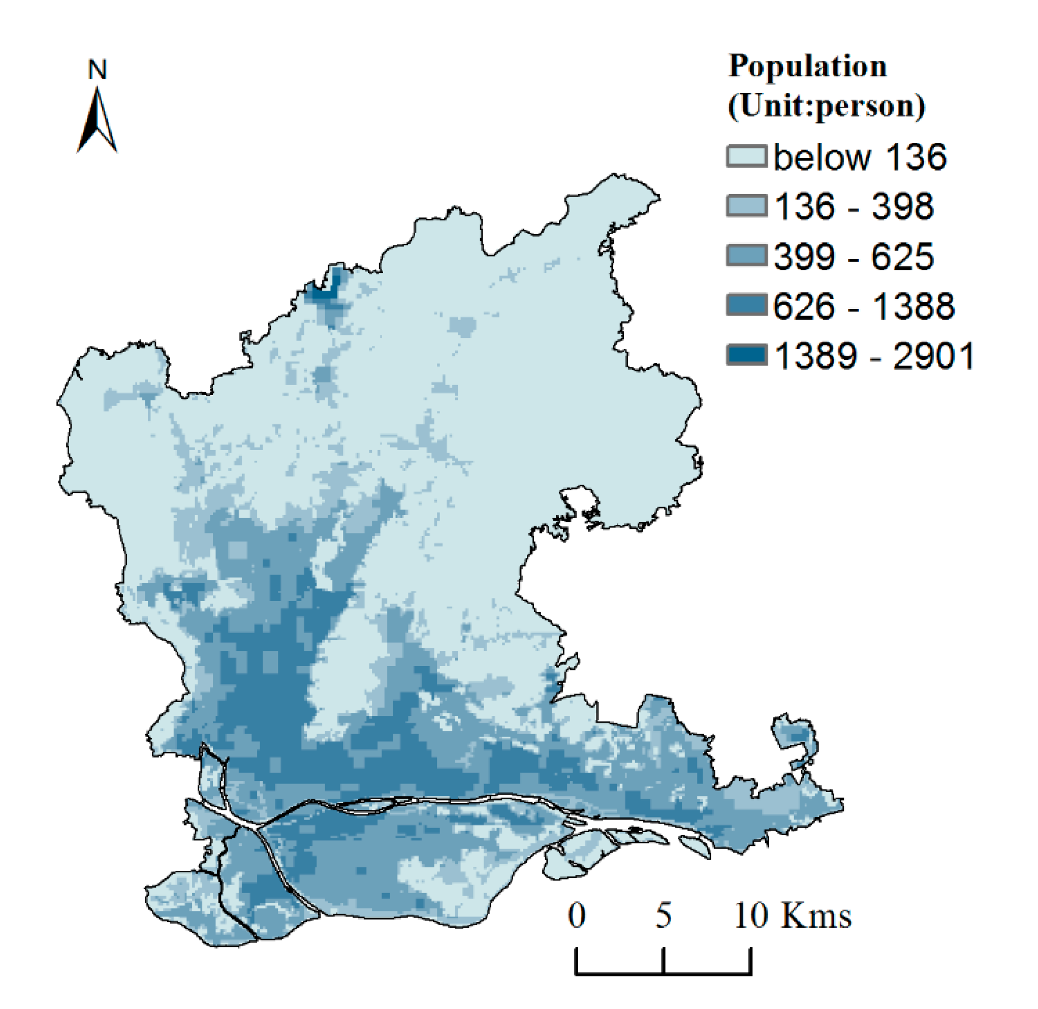
As shown in Figure 5, the population distribution in the study area presents an obvious “core-edge” pattern, i.e., the population is highly concentrated in the center of the study area, while the population density in the edge area is small. Among them, the northeast of Yuexiu district, Liwan district and Tianhe district has the largest population, and an aggregation effect is obvious. It is worth mentioning that the coefficient of determination (R2) of the random forest model result is 0.605, and the RMSE is 6497.02. At the same time, the average relative error of all streets (towns) in the study area is close to 32.16%. Compared with the global linear regression model, it can be seen that the simulation accuracy by using the random forest regression model has been significantly improved. However, for regions with large population density differences, a global model cannot accurately explain the mechanism of the spatial distribution of population.
3.3. Simulation Results by Using Zonal Strategy
3.3.1. Simulation Results for Dense Area
Dense area is located in the center of the city, and the population distribution is more affected by social and economic factors than natural environmental factors. To this end, sixteen impact factors were selected for population distribution modeling in dense area, including the road network density (X1), building area (X2), average house price (X3), catering facilities (X4), public facilities (X5), companies (X6), shopping facilities (X7), transportation facilities (X8), financial insurance (X9), scientific, educational and cultural facilities (X10), commercial residential buildings (X11), life service facilities (X12), sports and leisure facilities (X13), medical service facilities (X14), government agencies and society groups (X15), and accommodation facilities (X16).
The stepwise regression method was used to establish a multiple linear regression model for dense area. The model is shown as follows:
The random forest model was performed in the same way of global RF modelling as mentioned above. Ten-fold cross validation and grid search were conducted to find the proper parameters in the RF model for dense area. It is found that when the max depth of the decision tree was 10 and the number of estimators was 600, the determinant coefficient (R2) of the CV score reached the maximum value. Therefore, the random forest model was built, by setting the maximum depth of subtrees to 10, and the number of estimators to 600. Subsequently, the generated random forest regression model is applied to each grid cell to predict the population density in dense area. Finally, the simulation result is obtained by multiplying the population density and cell area. The two simulation results for dense area are shown in Figure 6, and their accuracy is shown in Table 5.
3.3.2. Simulation Results for Sparse Area
Compared with dense area, the factors affecting population density distribution in sparse area are more complex. On the one hand, it can be seen from the land use classification map that, due to the wide distribution and large area of cultivated land and forest land in sparse area, they should not be ignored in the modelling of population distribution. On the other hand, it can be seen from the digital elevation model that the elevation spatial differences in sparse area are obvious. Therefore, the natural environment and socio-economic factors should be fully considered in the process of selecting factors affecting the spatial distribution of population. Twenty impact factors are used as the main factors for spatial modeling of population in sparse area, including cultivated land index (X1), forest land index (X2), altitude (X3), building area (X4), road network density (X5), night light intensity (X6), housing price (X7), and point of interest (X8–X20).
The stepwise regression method was used to establish a multiple linear regression model for dense area. The model is shown as follows:
The random forest model was performed in the same way of global RF modelling as mentioned above. Ten-fold cross validation and grid search were conducted to find the proper parameters in the RF model for sparse area. It is found that when the max depth of the decision tree was 7 and the number of estimators was 600, the determinant coefficient (R2) of the CV score reached the maximum value. Therefore, the random forest model was built, by setting the maximum depth of subtrees to 7, and the number of estimators to 600. Subsequently, the generated random forest regression model is applied to each grid cell to predict the population density in sparse area. Finally, the simulation result is obtained by multiplying the population density and cell area. The two simulation results for sparse area are shown in Figure 7, and their accuracy is shown in Table 6.
3.3.3. Simulation Results for Whole Area
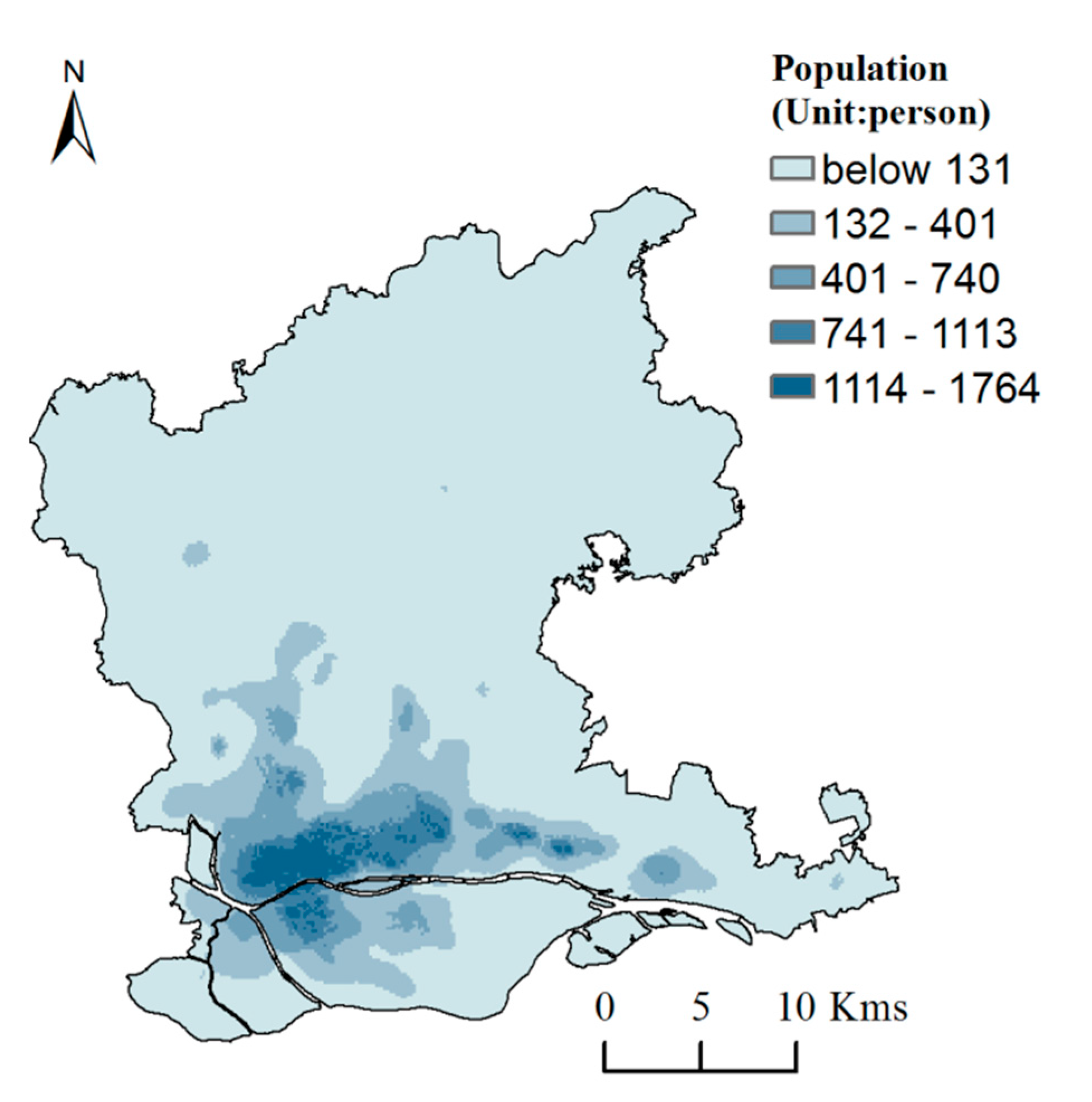
By merging the random forest simulation results of dense area and the linear regression simulation results of sparse area, the ultimate simulation result for whole study area is obtained (see Figure 8).
Comparing the simulation results by using the zonal model (Figure 8) with the simulation results by using the global LR model and global RF model (Figure 4 and Figure 5), it can be found that the simulation results based on zonal model strategy can reflect the spatial characteristics of the “core-periphery” population distribution in the study area more clearly. Taking the actual street population as the true value, the simulation accuracy of zonal model and global model were evaluated by using the goodness of fit. The results are shown in Table 7.
It can be seen from Table 7 that the simulation accuracy of zonal modeling is better than that of non-zonal models. Because the simulation accuracy of the single linear regression model is too low, it will not be discussed here. Next, the relative errors of the zonal model and the single random forest model were analyzed. The results are shown in Table 8.
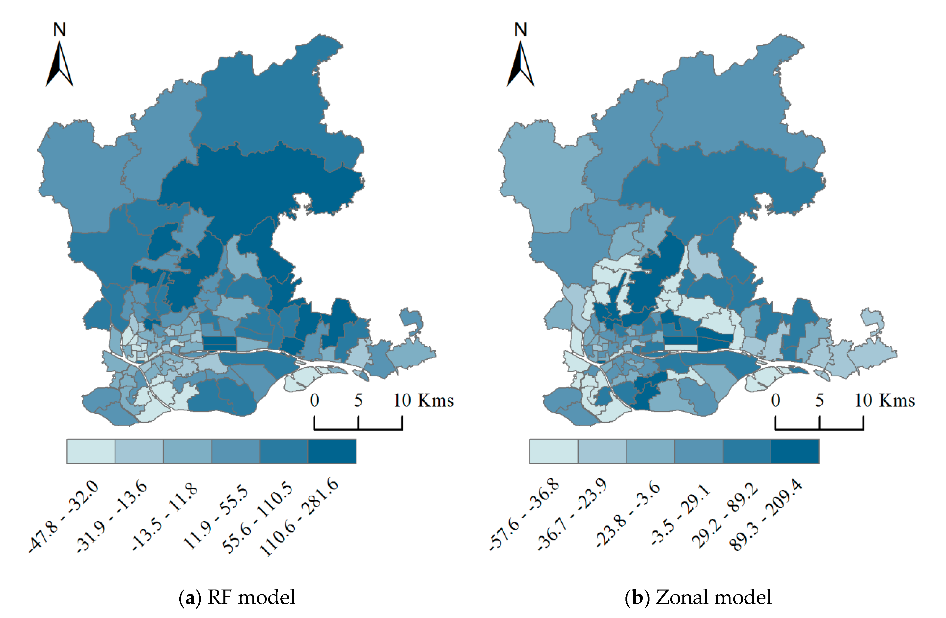
It can be seen from Table 8 that in the results of the zonal model, the proportion of streets with a simulation error within 30% is 51.89%, while the single random forest model is 49.06%. The difference between the two models is not obvious. However, in the modeling results, the proportion of streets with a relative error greater than 50% is 31.13% based on a single random forest model, which is obviously higher than the zonal model. Compared with the global random forest model, the proportion of streets with a relative error percentage greater than 50% in the zoning modeling results has decreased from 31.13% to 16.98%. In summary, the mapping results obtained based on the zonal modeling strategy are more in line with the actual situation, which can significantly improve the accuracy of population distribution mapping. Thematic maps are drawn for the relative error percentage values of each street produced by two models. The thematic maps are shown in Figure 9.
It can be seen from Figure 9 that, the accuracy of simulation results in the region including Baiyun district, the east of Tianhe district, and Huangpu district are lower than other regions. The relative error percentages of streets in these area are mostly exceeding 50%. Among them, Tonghe street in Baiyun district has the highest MRE in the global random forest model result, while Sanyuanli street in Baiyun district has the highest MRE in the zonal model result. Although different models were applied to different subareas in this paper, due to the obvious differences in the natural environment and social-economic development level between two subareas. However, in the dense area, whether global random forest or zonal model, the model accuracy is relatively low. A reasonable estimation is that as densely populated areas are areas are usually with rapid urbanization rate, the mismatch of temporal and spatial resolutions of different data sources may cause large deviations between model results and statistical data. This inadequacy may reduce the simulation accuracy of the model.
4. Discussion and Conclusions
4.1. Discussion
As for the census data of administrative units, it shows how many people are distributed in a certain spatial range (e.g., a county or a township), and where the specific distribution cannot be presented. That is, census data is not designed for the purpose of spatialization, and the mapping based on grid units can achieve the fine mapping of population distribution [41]. Therefore, the gridded population mapping is very important for urban management. However, previous studies on fine-scale population mapping are few, and the spatial resolutions of mapping results are mostly based on a grid with a 500 m or 1 km spatial resolution, which is difficult to meet the requirements of fine management. This study produced the 150 m gridded population data in central Guangzhou using the strategy of zoning modeling integrated two machine learning methods. The state-of-the-art random forest model and linear regression model were used to integrate multiple data and predict the population density distribution, which was used for the gridded population mapping. The results provide timely and important information to policy makers for city management and planning [51]. Obviously, the maps with grid units are visually coarse and cannot produce the information consisting of the geographical entities (i.e., the human residential settlements). On the contrary, our mapping result can provide fine population information by using homogeneous polygons with irregular boundaries. On the basis of the above experimental analysis, it is necessary to further discuss the following issues.
4.1.1. Principal Findings and Meaningful Implication
- (1)
- The geographic detector model is a very useful tool for identification of influence factor on population density distribution. As many concerned natural and socioeconomic variables were input in our modeling, the analysis of the geographic detector model has an obvious positive effect on understanding the mechanism of influencing population distribution in this study area. The experimental results of population distribution mapping show that the influence factors selected by the geographic detector model are reasonable. However, the impact factor selected by the geographic detector model is not the final modeling factors for linear regression model. The explanatory power ranking results demonstrated that socioeconomic factors have a greater impact on the spatial distribution of population in the study area than natural factors. This finding is consistent with previous studies.
- (2)
- The zoning modeling strategy using machine learning methods can improve the accuracy of fine-scale population mapping in urbanized areas. The results show that the goodness of fit for the zoning model result is close to 0.713, while the goodness of fit for single linear regression model and random forest regression model are 0.0039 and 0.605, respectively. We speculate that the poor accuracy of the single linear regression model is mainly due to the low spatial resolution of land use data and the insufficient classification of types, which leads to large deviations in the simulation results. Compared with zonal model, the reason for the lower accuracy of the global random forest model may be due to the neglect of the natural and human environment differences between dense area and sparse area. For dense area, the accuracy of the random forest model is better than the linear regression model. While for sparse area, the accuracy of the linear regression model is better than the random forest model. Compared with the linear regression model, although the random forest model has many advantages in theory, it does not guarantee that it has an accuracy advantage in population distribution mapping. Therefore, it is advised that the zonal modeling strategy should be the first choice for solving regional differences in the population distribution mapping research.
- (3)
- The application of random forest regression in fine-scale population mapping should be cautious. Despite the random forest model is popularized in many disciplines as its advantages, some major and crucial parameters can affect the results achieved by users [58,59], such as max depth of the decision trees, the max number of features, and so on. Therefore, tuning the parameters is a crucial work in random forest modelling. Grid search combined with K-fold cross-validation is an effective method to find the optimal parameters, especially when the number of sample is small. As the number of streets being used to fit the model is only 106, 10-fold CV was chosen in our study. The prediction result has a good effect with the goodness of fit value of 0.605 in the global random forest model.
4.1.2. Explanations for Further Research
Fine-scale population distribution mapping is a very complicated problem. This paper first uses the geographic detector model to select the influencing factors on population spatial distribution, and then realizes the population distribution mapping using the single model and zoning model, and finally compares the simulation results to prove that the accuracy of the zonal method implemented in this paper has been improved significantly. However, due to the limitation of personal scientific research ability, time, and other factors, there are still the following shortcomings in the research process of this article, which need to be gradually improved in the future.
- (1)
- The quality of data source for modeling can be improved. The spatial resolution of NPP/VIIRS night light data is nearly 500 m, which is too coarse for population mapping in city or commune scale. Compared to NPP-VIIRS data, spatial resolution and quantitative level of LJ 1-01 data have increased from 500 m to 150 m. Despite the finest resolution of the LJ 1-01 data, the complex urban fabric patterns and the uncertainty of the radiation calibration of Luojia1-01 constrain the application of the images in conducting accurate population estimations at a fine scale. Besides that, the spatial and type resolution of land use data used in this paper are also not detailed enough, which may affect the accuracy of the model obviously. Moreover, the time characteristics of the data source do not match. The street (town) demographic data used in the research is from 2013, while the land use, night lighting, POI, and other data used in the modeling are later than 2015. The mismatch of the time characteristics will inevitably affect the accuracy of the model. Therefore, application of more detailed and accurate dataset in population mapping should be further studied as soon as possible.
- (2)
- The issue of model uncertainty need be addressed in further studies. Similar to many studies, different model parameters produce different model results, especially in the field of geography science. For example, grid size may affect the model result. The gridded population data with appropriate cell size can reveal the spatial varieties of population distribution pattern more clearly. According to previous research experience, in order to prevent the smallest residential units from falling into the same grid, the grid size is set to 150 m in our study. However, whether there is a more suitable grid size for the model is still to be studied. As we know, sensitivity analysis is a useful method to explore the uncertainty of modelling. Consequently, the issue of uncertainty using sensitivity analysis method in the population mapping is another topic need to be explored.
- (3)
- There is still potential for improvement in the selection of modeling factors. In fact, the influence mechanism of population distribution is a tough topic. Although this paper identified the main influence factors by integrating previous experience with geographic detector model analysis, it is still difficult to fully reveal the inherent mechanism. For example, random forest model can also be used to distinguish the importance of different features [60]. Among the impact factors selected in this article, POI data accounted for the vast majority, which has an extremely important impact on the modeling of population distribution. Meanwhile, each category of POI may be correlated with each other, which may cause some feature importance bias. Further studies must deal with the independence of each feature or fitting the model by integrating all the POIs into one layer.
Besides that, only two classic machine learning methods such as linear regression and random forest are used in this paper. The applicability and accuracy evaluation of other machine learning methods such as neural networks, support vector machine, and so on, should to be further studied. In other words, more efforts are needed to apply alternative ways to build new models with proper parameters.
4.2. Conclusions
This study provided a zonal method for downscaling the census population to 30 m’ grid scale in central Guangzhou, China. Firstly, the geographic detector model is used to select the influencing factors on population spatial distribution. Then, the population distribution mapping with the single model and zoning model are realized respectively. Finally, the accuracies of different model result are compared. The street-level accuracy evaluation results show that, the proposed approach achieved good overall accuracy, with R2 being 0.713 and RMSE being 5512.9. Meanwhile, the goodness of fit for single linear regression model and random forest regression model are 0.0039 and 0.605 respectively. Our study demonstrated that the accuracy of the population distribution mapping can be effectively improved compared with mapping which does not use the zoning modeling strategy. The results indicated that the proposed method has great potential in fine-scale population mapping. For dense area, the accuracy of the random forest model is better than the linear regression model. For sparse area, the accuracy of the linear regression model is better than the random forest model. Therefore, it is advised that the zonal modeling strategy should be the first choice for solving regional differences in the population distribution mapping research.
Author Contributions
Conceptualization, Guanwei Zhao and Muzhuang Yang; Methodology, Guanwei Zhao and Muzhuang Yang; Software, Guanwei Zhao; Validation, Guanwei Zhao; Formal Analysis, Guanwei Zhao; Investigation, Guanwei Zhao; Resources, Guanwei Zhao and Muzhuang Yang; Data Curation, Guanwei Zhao; Writing—Original Draft Preparation, Guanwei Zhao and Muzhuang Yang; Writing—Review & Editing, Guanwei Zhao and Muzhuang Yang; Visualization, Guanwei Zhao and Muzhuang Yang; Supervision, Muzhuang Yang. All authors have read and agreed to the published version of the manuscript.
Funding
This research was funded in part by Natural Science Foundation of Guangdong Province, China: Grant Number 2017A030313240, Philosophy and Social Science Research Program of Guangzhou city, Guangdong Province, China: Grant Number 2020GZGJ183, and Guangzhou Science and Technology Plan Project—Joint Project Funding by City and University (The project name is fine simulation of population distribution in Guangzhou city considering scale effect, but the project number has not yet been announced).
Acknowledgments
The authors appreciate the work of the editor and the reviewers.
Conflicts of Interest
The authors declare no conflict of interest. The funders had no role in the design of the study; in the collection, analyses, or interpretation of data; in the writing of the manuscript, or in the decision to publish the results.
References
- Yang, X.; Yue, W.; Gao, D. Spatial improvement of human population distribution based on multi-sensor remote-sensing data: An input for exposure assessment. Int. J. Remote Sens. 2013, 34, 5569–5583. [Google Scholar] [CrossRef]
- Zhao, Y.; Ovando-Montejo, G.A.; Frazier, A.E.; Mathews, A.J.; Flynn, K.C.; Ellis, E.A. Estimating work and home population using lidar-derived building volumes. Int. J. Remote Sens. 2017, 38, 1180–1196. [Google Scholar] [CrossRef]
- Maantay, J.A.; Maroko, A.R.; Herrmann, C. Mapping Population Distribution in the Urban Environment: The Cadastral-based Expert Dasymetric System (CEDS). Cartogr. Geogr. Inf. Sci. 2007, 34, 77–102. [Google Scholar] [CrossRef]
- Martin, D.; Lloyd, C.; Shuttleworth, I. An evaluation of gridded population models using 2001 Northern Ireland census data. Environ. Plan. 2011, 43, 1965–1980. [Google Scholar] [CrossRef]
- Lung, T.; Lübker, T.; Ngochoch, J.K.; Schaab, G. Human population distribution modelling at regional level using very high resolution satellite imagery. Appl. Geogr. 2013, 41, 36–45. [Google Scholar] [CrossRef]
- Aubrecht, C.; Aubrecht, D.O.; Ungar, J.; Freire, S.; Steinnocher, K. VGDI—Advancing the Concept: Volunteered Geo-Dynamic Information and its Benefits for Population Dynamics Modeling. Trans. Gis 2017, 21, 253–276. [Google Scholar] [CrossRef]
- Jia, P.; Gaughan, A.E. Dasymetric modeling: A hybrid approach using land cover and tax parcel data for mapping population in Alachua County, Florida. Appl. Geogr. 2016, 66, 100–108. [Google Scholar] [CrossRef]
- Li, G.; Weng, Q. Using Landsat ETM+ Imagery to Measure Population Density in Indianapolis, Indiana, USA. Photogramm. Eng. Remote Sens. 2005, 71, 947–958. [Google Scholar] [CrossRef]
- Calka, B.; Nowak Da Costa, J.; Bielecka, E. Fine scale population density data and its application in risk assessment. Geomat. Nat. Hazards Risk 2017, 8, 1440–1455. [Google Scholar] [CrossRef]
- Freire, S.; Schiavina, M.; Florczyk, A.J.; MacManus, K.; Pesaresi, M.; Corbane, C.; Borkovska, O.; Mills, J.; Pistolesi, L.; Squires, J.; et al. Enhanced data and methods for improving open and free global population grids: Putting ’leaving no one behind’ into practice. Int. J. Digit. Earth 2020, 13, 61–77. [Google Scholar] [CrossRef] [Green Version]
- Azar, D.; Engstrom, R.; Graesser, J.; Comenetz, J. Generation of fine-scale population layers using multi-resolution satellite imagery and geospatial data. Remote Sens. Environ. 2013, 130, 219–232. [Google Scholar] [CrossRef]
- Reed, F.J.; Gaughan, A.E.; Stevens, F.R.; Yetman, G.; Sorichetta, A.; Tatem, A.J. Gridded Population Maps Informed by Different Built Settlement Products. Data 2018, 3, 33. [Google Scholar] [CrossRef] [Green Version]
- Ye, T.; Zhao, N.; Yang, X.; Ouyang, Z.; Liu, X.; Chen, Q.; Hu, K.; Yue, W.; Qi, J.; Li, Z.; et al. Improved population mapping for China using remotely sensed and points-of-interest data within a random forests model. Sci. Total Environ. 2019, 658, 936–946. [Google Scholar] [CrossRef]
- Flowerdew, R.; Green, M. Developments in areal interpolation methods and GIS. Ann. Reg. Sci. 1992, 26, 67–78. [Google Scholar] [CrossRef]
- Goodchild, M.F.; Anselin, L.; Deichmann, U.A. Framework for the Areal Interpolation of Socioeconomic Data. Environ. Plan. A Econ. Space 1993, 25, 383–397. [Google Scholar] [CrossRef]
- Mennis, J. Generating Surface Models of Population Using Dasymetric Mapping. Prof. Geogr. 2003, 55, 31–42. [Google Scholar]
- Tobler, W.; Deichmann, U.; Gottsegen, J.; Maloy, K. World Population in a Grid of Spherical Quadrilaterals. Int. J. Popul. Geogr. 1997, 3, 203–225. [Google Scholar] [CrossRef]
- Lin, J.; Cromley, R.G. Evaluating geo-located Twitter data as a control layer for areal interpolation of population. Appl. Geogr. 2015, 58, 41–47. [Google Scholar] [CrossRef]
- Shi, X.; Li, M.; Hunter, O.; Guetti, B.; Andrew, A.; Stommel, E.; Bradley, W.; Karagas, M.R. Estimation of environmental exposure: Interpolation, kernel density estimation or snapshotting. Ann. GIS 2019, 25, 1–8. [Google Scholar] [CrossRef] [Green Version]
- Lam, N.S.N. Spatial Interpolation Methods: A Review. Am. Cartogr. 1983, 10, 129–149. [Google Scholar] [CrossRef]
- Wu, C.; Murray, A.T. A cokriging method for estimating population density in urban areas. Comput. Environ. Urban. Syst. 2005, 29, 558–579. [Google Scholar] [CrossRef]
- Langford, M.; Unwin, D.J. Generating and mapping population density surfaces within a geographical information system. Cartogr. J. 1994, 31, 21–26. [Google Scholar] [CrossRef] [PubMed]
- Gaughan, A.E.; Stevens, F.R.; Linard, C.; Jia, P.; Tatem, A.J. High Resolution Population Distribution Maps for Southeast Asia in 2010 and 2015. PLoS ONE 2013, 8, e55882. [Google Scholar] [CrossRef] [PubMed]
- Jia, P.; Qiu, Y.; Gaughan, A.E. A fine-scale spatial population distribution on the High-resolution Gridded Population Surface and application in Alachua County, Florida. Appl. Geogr. 2014, 50, 99–107. [Google Scholar] [CrossRef]
- Townsend, A.C.; Bruce, D.A. The use of night-time lights satellite imagery as a measure of Australia’s regional electricity consumption and population distribution. Int. J. Remote Sens. 2010, 31, 4459–4480. [Google Scholar] [CrossRef]
- Briggs, D.J.; Gulliver, J.; Fecht, D.; Vienneau, D.M. Dasymetric modelling of small-area population distribution using land cover and light emissions data. Remote Sens. Environ. 2007, 108, 451–466. [Google Scholar] [CrossRef]
- Chen, Y.; Zheng, Z.; Wu, Z.; Qian, Q. Review and prospect of application of nighttime light remote sensing data. Adv. Earth Sci. 2019, 38, 205–223. [Google Scholar]
- Chen, Z.; Yu, B.; Hu, Y.; Huang, C.; Shi, K.; Wu, J. Estimating House Vacancy Rate in Metropolitan Areas Using NPP-VIIRS Nighttime Light Composite Data. IEEE J. Sel. Top. Appl. Earth Obs. Remote Sens. 2015, 8, 2188–2197. [Google Scholar] [CrossRef]
- Zhou, Q.; Zheng, Y.; Shao, J.; Lin, Y.; Wang, H. An Improved Method of Determining Human Population Distribution Based on Luojia 1-01 Nighttime Light Imagery and Road Network Data—A Case Study of the City of Shenzhen. Sensors 2020, 20, 5032. [Google Scholar] [CrossRef]
- Sutton, K.; Roberts, D.; Elvidge, C. Census from Heaven: An estimate of the global human population using night-time satellite imagery. Int. J. Remote Sensing 2001, 22, 3061–3076. [Google Scholar] [CrossRef]
- Li, X.; Zhao, L.; Li, D.; Xu, H. Mapping Urban Extent Using Luojia 1-01 Nighttime Light Imagery. Sensors 2018, 18, 3665. [Google Scholar] [CrossRef] [Green Version]
- Jiang, W.; He, G.; Long, T.; Guo, H.; Yin, R.; Leng, W.; Liu, H.; Wang, G. Potentiality of Using Luojia 1-01 Nighttime Light Imagery to Investigate Artificial Light Pollution. Sensors 2018, 18, 2900. [Google Scholar] [CrossRef] [Green Version]
- Li, F.; Yan, Q.; Bian, Z.; Liu, B.; Wu, Z. A POI and LST Adjusted NTL Urban Index for Urban Built-Up Area Extraction. Sensors 2020, 20, 2918. [Google Scholar] [CrossRef]
- Wu, T.J.; Luo, J.C.; Dong, W.; Gao, L.J.; Hu, X.D.; Wu, Z.F.; Sun, Y.W.; Liu, J.S. Disaggregating County-Level Census Data for Population Mapping Using Residential Geo-Objects With Multisource Geo-Spatial Data. IEEE J. Sel. Top. Appl. Earth Obs. Remote Sens. 2020, 13, 1189–1205. [Google Scholar] [CrossRef]
- Xiong, J.N.; Li, K.; Cheng, W.M.; Ye, C.C.; Zhang, H. A Method of Population Spatialization Considering Parametric Spatial Stationarity: Case Study of the Southwestern Area of China. ISPRS Int. J. Geo Inf. 2019, 8, 495. [Google Scholar] [CrossRef] [Green Version]
- Wang, L.T.; Wang, S.X.; Zhou, Y.; Liu, W.L.; Hou, Y.F.; Zhu, J.F.; Wang, F.T. Mapping population density in China between 1990 and 2010 using remote sensing. Remote Sens. Environ. 2018, 210, 269–281. [Google Scholar] [CrossRef]
- Bakillah, M.; Liang, S.; Mobasheri, A.; Jokar Arsanjani, J.; Zipf, A. Fine-resolution population mapping using OpenStreetMap points-of-interest. Int. J. Geogr. Inf. Sci. 2014, 28, 1940–1963. [Google Scholar] [CrossRef]
- Ma, Y.J.; Xu, W.; Zhao, X.J.; Li, Y. Modeling the Hourly Distribution of Population at a High Spatiotemporal Resolution Using Subway Smart Card Data: A Case Study in the Central Area of Beijing. ISPRS Int. J. Geo-Inf. 2017, 6, 128. [Google Scholar] [CrossRef] [Green Version]
- Song, J.C.; Tong, X.Y.; Wang, L.Z.; Zhao, C.L.; Prishchepov, A.V. Monitoring finer-scale population density in urban functional zones: A remote sensing data fusion approach. Landsc. Urban. Plan. 2019, 190, 103580. [Google Scholar] [CrossRef]
- Yu, B.; Lian, T.; Huang, Y.; Yao, S.; Ye, X.; Chen, Z.; Yang, C.; Wu, J. Integration of nighttime light remote sensing images and taxi GPS tracking data for population surface enhancement. Int. J. Geogr. Inf. Sci. 2019, 33, 687–706. [Google Scholar] [CrossRef]
- Shi, Y.; Yang, J.; Shen, P. Revealing the Correlation between Population Density and the Spatial Distribution of Urban Public Service Facilities with Mobile Phone Data. ISPRS Int. J. Geo Inf. 2020, 9, 38. [Google Scholar] [CrossRef] [Green Version]
- Yao, Y.; Liu, X.; Li, X.; Zhang, J.; Liang, Z.; Mai, K.; Zhang, Y. Mapping fine-scale population distributions at the building level by integrating multisource geospatial big data. Int. J. Geogr. Inf. Sci. 2017, 31, 1220–1244. [Google Scholar] [CrossRef]
- Li, J.; Li, J.; Yuan, Y.; Li, G. Spatiotemporal distribution characteristics and mechanism analysis of urban population density: A case of Xi’an, Shaanxi, China. Cities 2019, 86, 62–70. [Google Scholar] [CrossRef]
- Azar, D.; Graesser, J.; Engstrom, R.; Comenetz, J.; Leddy, R.M.; Schechtman, N.G.; Andrews, T. Spatial refinement of census population distribution using remotely sensed estimates of impervious surfaces in Haiti. Int. J. Remote Sens. 2010, 31, 5635–5655. [Google Scholar] [CrossRef]
- Breiman, L. Random Forests. Mach. Learn. 2001, 45, 5–32. [Google Scholar] [CrossRef] [Green Version]
- Gao, N.; Li, F.; Zeng, H.; Van Bilsen, D.; De Jong, M. Can More Accurate Night-Time Remote Sensing Data Simulate a More Detailed Population Distribution? Sustainability 2019, 11, 4488. [Google Scholar] [CrossRef] [Green Version]
- Deville, P.; Linard, C.; Martin, S.; Gilbert, M.; Stevens, F.R.; Gaughan, A.E.; Blondel, V.D.; Tatem, A.J. Dynamic population mapping using mobile phone data. Proc. Natl. Acad. Sci. USA 2014, 111, 15888–15893. [Google Scholar] [CrossRef] [Green Version]
- Stevens, F.R.; Gaughan, A.E.; Linard, C.; Tatem, A.J. Disaggregating census data for population mapping using random forests with remotely-sensed and ancillary data. PLoS ONE 2015, 10, e0107042. [Google Scholar] [CrossRef] [Green Version]
- Criminisi, A.; Shotton, J.; Konukoglu, E. Decision forests: A unified framework for classification, regression, density estimation, manifold learning and semi-supervised learning. Found. Trends Comput. Graph. Vis. 2011, 7, 81–227. [Google Scholar] [CrossRef]
- Boulesteix, A.-L.; Janitza, S.; Kruppa, J.; König, I.R. Overview of random forest methodology and practical guidance with emphasis on computational biology and bioinformatics. Wiley Interdiscip. Rev. Data Min. Knowl. Discov. 2012, 2, 493–507. [Google Scholar] [CrossRef] [Green Version]
- Zhou, Y.; Ma, M.; Shi, K.; Peng, Z. Estimating and Interpreting Fine-Scale Gridded Population Using Random Forest Regression and Multisource Data. ISPRS Int. J. Geo Inf. 2020, 9, 369. [Google Scholar] [CrossRef]
- Rodrigues, A.M.; Tenedório, J.A. Sensitivity Analysis of Spatial Autocorrelation Using Distinct Geometrical Settings: Guidelines for the Quantitative Geographer. Int. J. Agric. Environ. Inf. Syst. IJAEIS 2016, 7, 13. [Google Scholar] [CrossRef] [Green Version]
- Bai, Z.Q.; Wang, J.L.; Wang, M.M.; Gao, M.X.; Sun, J.L. Accuracy Assessment of Multi-Source Gridded Population Distribution Datasets in China. Sustainability 2018, 10, 1363. [Google Scholar] [CrossRef] [Green Version]
- Wang, J.F.; Li, X.H.; Christakos, G.; Liao, Y.L.; Zhang, T.; Gu, X.; Zheng, X.Y. Geographical Detectors-Based Health Risk Assessment and its Application in the Neural Tube Defects Study of the Heshun Region, China. Int. J. Geogr. Inf. Sci. 2010, 24, 107–127. [Google Scholar] [CrossRef]
- Oh, Y.J.; Park, H.S.; Min, Y. Understanding location-based service application connectedness: Model development and cross-validation. Comput. Hum. Behav. 2019, 94, 82–91. [Google Scholar] [CrossRef]
- Gholinejad, S.; Naeini, A.A.; Amiri-Simkooei, A.R. Robust Particle Swarm Optimization of RFMs for High-Resolution Satellite Images Based on K-Fold Cross-Validation. IEEE J. Sel. Top. Appl. Earth Obs. Remote. Sens. 2019, 12, 2594–2599. [Google Scholar] [CrossRef]
- Liu, R.; Feng, Z.; Yang, Y.; You, Z. Research on the Spatial Pattern of Population Agglomeration and Dispersion in China. Prog. Geogr. 2010, 29, 1171–1177. (In Chinese) [Google Scholar]
- Biau, G.; Scornet, E. A Random Forest Guided Tour. Test 2016, 25, 197–227. [Google Scholar] [CrossRef] [Green Version]
- Grömping, U. Variable Importance Assessment in Regression: Linear Regression versus Random Forest. Am. Stat. 2009, 63, 308–319. [Google Scholar] [CrossRef]
- Gregorutti, B.; Michel, B.; Saint-Pierre, P. Correlation and variable importance in random forests. Stat. Comput. 2017, 27, 659–678. [Google Scholar] [CrossRef] [Green Version]
Figure 1.
Population density map of the study area in 2013.
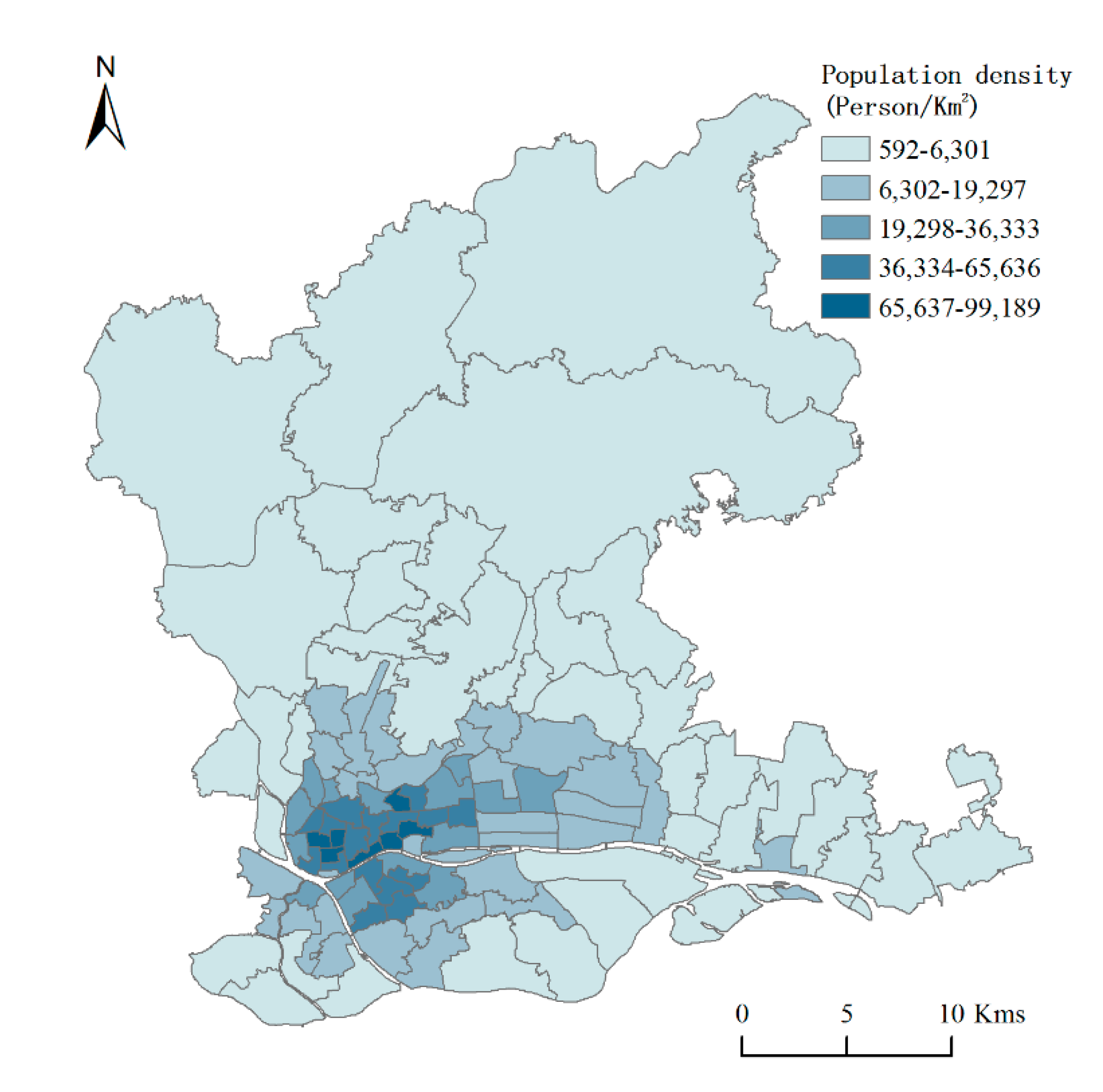
Figure 2.
Explanatory power of influencing factors on population density.

Figure 3.
Zoning map of the research area based on population congregation.

Figure 4.
Simulation result by using global linear regression model.

Figure 5.
Simulation result by using global random forest regression model.

Figure 6.
Population distribution maps in dense area.

Figure 7.
Population distribution maps in sparse area.

Figure 8.
Population distribution map in the study area.
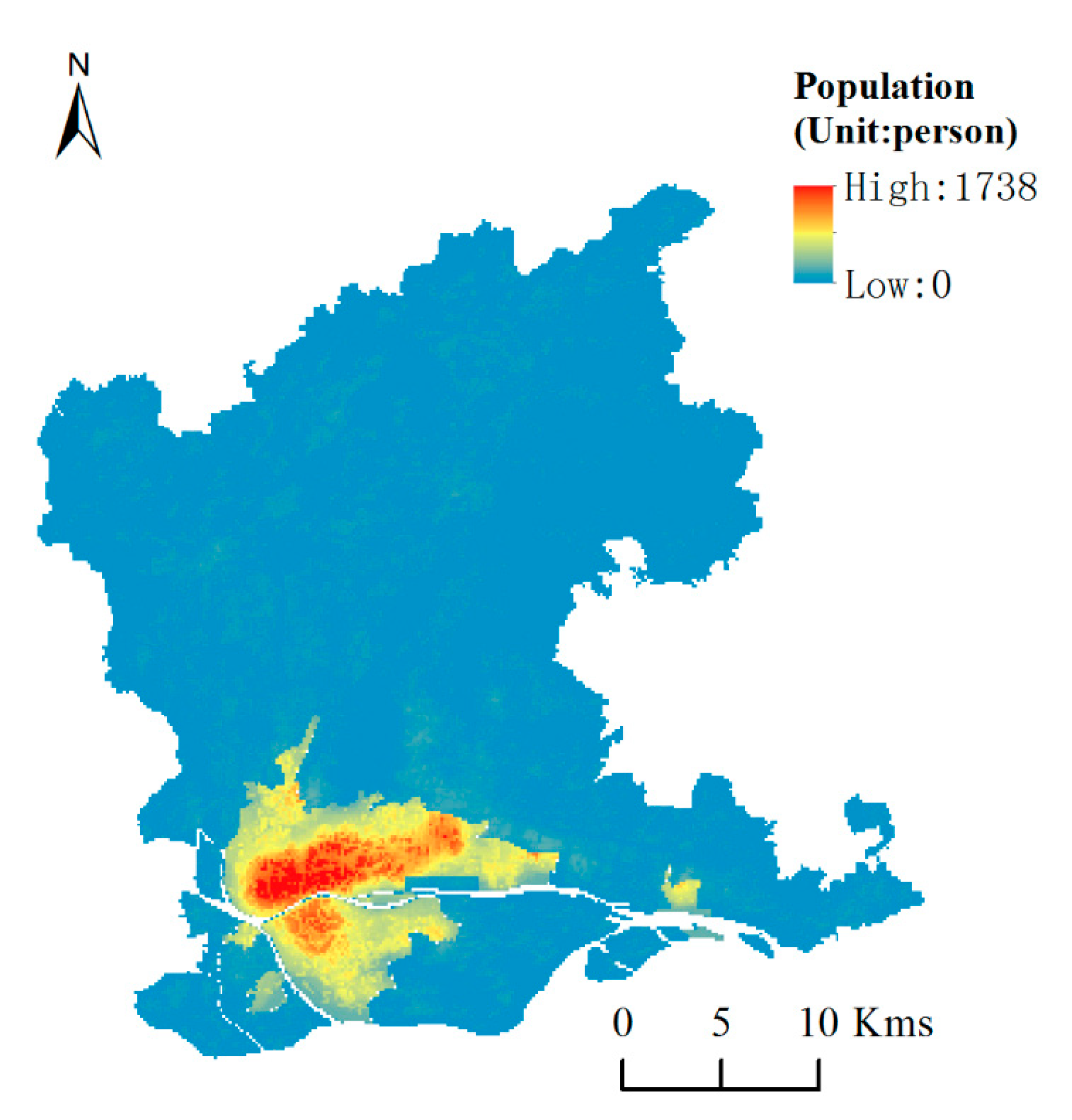
Figure 9.
Distribution map of mean relative error (MRE) in two models.


Table 1.
Data Source Information.
| Data | Acquisition Method | Year |
|---|---|---|
| Administrative boundaries data | Digitization based on Gaode map | 2014 |
| Census data | Provided by Guangzhou Municipal Public Security Bureau | 2013 |
| Digital elevation model (DEM) data | http://www.gscloud.cn/search | 2009 |
| Land use data | http://www.resdc.cn/ | 2015 |
| Roads data | Digitization based on Gaode map | 2014 |
| Point of interest (POI) data | Collected from Baidu Map | 2018 |
| Night light data | https://ngdc.noaa.gov/eog/viirs/download_dnb_composites.html | 2016 |
| Building area data | Collected from Baidu Map | 2015 |
| Housing price data | Collected from Lianjia’s website | 2018 |
Table 2.
Data Source Information.
| Data | Calculation Methods |
|---|---|
| Road Index () | denotes the road length in the grid cell i, denotes the area of grid cell i |
| Land use Index () | , denotes the area of land use type j in grid cell i, denotes the total area of land use polygons in grid cell i |
| Night light Index () | The average value of night light intensity of grid cell i |
| Elevation Index () | The average elevation value of grid cell i |
| Building Index () | , denotes the building area of grid cell i, is the area of grid cell i |
| POI Index () | The average density of each types of POI data in the grid cell i |
| House price index () | The average house price in the grid cell i |
Table 3.
Variance analysis results.
| df | SS | MS | F | Significance F | |
|---|---|---|---|---|---|
| Model | 7 | 62,369,873,618.10 | 8,909,981,945 | 19.7687925 | 2.74802 × 10⁻¹⁶ |
| Residual | 99 | 44,620,237,303.76 | 450,709,467.7 | ||
| Total | 106 | 1.0699 × 10¹¹ |
Table 4.
The ten-fold cross validation for the proper parameters in the random forest.
| n_estimators | max_depth | ||||||||
|---|---|---|---|---|---|---|---|---|---|
| 2 | 3 | 4 | 5 | 6 | 7 | 8 | 9 | 10 | |
| 200 | 0.6558 | 0.7189 | 0.7212 | 0.7215 | 0.7206 | 0.7210 | 0.7219 | 0.7204 | 0.7185 |
| 300 | 0.6558 | 0.7208 | 0.7197 | 0.7221 | 0.7201 | 0.7198 | 0.7199 | 0.7195 | 0.7180 |
| 400 | 0.6591 | 0.7217 | 0.7219 | 0.7239 | 0.7225 | 0.7212 | 0.7221 | 0.7222 | 0.7211 |
| 500 | 0.6599 | 0.7233 | 0.7236 | 0.7245 | 0.7245 | 0.7235 | 0.7239 | 0.7250 | 0.7227 |
| 600 | 0.6581 | 0.7210 | 0.7226 | 0.7219 | 0.7228 | 0.7213 | 0.7214 | 0.7234 | 0.7211 |
| 700 | 0.6586 | 0.7211 | 0.7222 | 0.7220 | 0.7226 | 0.7210 | 0.7211 | 0.7231 | 0.7213 |
| 800 | 0.6568 | 0.7203 | 0.7221 | 0.7213 | 0.7223 | 0.7212 | 0.7206 | 0.7218 | 0.7207 |
| 900 | 0.6567 | 0.7208 | 0.7219 | 0.7212 | 0.7220 | 0.7209 | 0.7206 | 0.7218 | 0.7208 |
| 1000 | 0.6554 | 0.7202 | 0.7220 | 0.7209 | 0.7214 | 0.7206 | 0.7201 | 0.7210 | 0.7203 |
Table 5.
Model accuracy in dense area.
| Model | R2 | MRE | RMSE |
|---|---|---|---|
| LR | 0.343 | 29.28% | 16,068.09 |
| RF | 0.445 | 26.12% | 12,385.07 |
Table 6.
Model accuracy in sparse area.
| Model | R2 | MRE | RMSE |
|---|---|---|---|
| LR | 0.847 | 13.09% | 692.45 |
| RF | 0.752 | 15.67% | 779.93 |
Table 7.
Model accuracy in the whole area.
| Model | R2 | MRE (%) | RMSE |
|---|---|---|---|
| Zonal Model | 0.713 | 12.87 | 5512.90 |
| Global Linear Regression | 0.004 | 235.98 | 1,007,871.35 |
| Global Random Forest | 0.605 | 32.16 | 6497.02 |
Table 8.
Error statistics for models in the whole area.
| Model | RE (%) | Amount of Street | Percentage (%) |
|---|---|---|---|
| Zonal Model | <−50% | 4 | 3.77 |
| −50%30% | 20 | 18.87 | |
| −30%0 | 35 | 33.02 | |
| 030% | 20 | 18.87 | |
| 30%50% | 13 | 12.26 | |
| >50% | 14 | 13.21 | |
| Random Forest | <−50% | 0 | 0 |
| −50%30% | 13 | 12.26 | |
| −30%0 | 31 | 29.25 | |
| 030% | 21 | 19.81 | |
| 30%50% | 8 | 7.55 | |
| >50% | 33 | 31.13 |
Publisher’s Note: MDPI stays neutral with regard to jurisdictional claims in published maps and institutional affiliations. |
© 2020 by the authors. Licensee MDPI, Basel, Switzerland. This article is an open access article distributed under the terms and conditions of the Creative Commons Attribution (CC BY) license (http://creativecommons.org/licenses/by/4.0/).
Share and Cite
MDPI and ACS Style
Zhao, G.; Yang, M. Urban Population Distribution Mapping with Multisource Geospatial Data Based on Zonal Strategy. ISPRS Int. J. Geo-Inf. 2020, 9, 654. https://0-doi-org.brum.beds.ac.uk/10.3390/ijgi9110654
AMA Style
Zhao G, Yang M. Urban Population Distribution Mapping with Multisource Geospatial Data Based on Zonal Strategy. ISPRS International Journal of Geo-Information. 2020; 9(11):654. https://0-doi-org.brum.beds.ac.uk/10.3390/ijgi9110654
Chicago/Turabian StyleZhao, Guanwei, and Muzhuang Yang. 2020. "Urban Population Distribution Mapping with Multisource Geospatial Data Based on Zonal Strategy" ISPRS International Journal of Geo-Information 9, no. 11: 654. https://0-doi-org.brum.beds.ac.uk/10.3390/ijgi9110654
Note that from the first issue of 2016, this journal uses article numbers instead of page numbers. See further details here.