A Fuzzy Spatial Region Extraction Model for Object’s Vague Location Description from Observer Perspective

1
Jilin Provincial Key Laboratory of Changbai Historical Culture and VR Reconstruction Technology, Changchun Institute of Technology, Changchun 130012, China
2
School of Computer Technology and Engineering, Changchun Institute of Technology, Changchun 130012, China
*
Author to whom correspondence should be addressed.
ISPRS Int. J. Geo-Inf. 2020, 9(12), 703; https://0-doi-org.brum.beds.ac.uk/10.3390/ijgi9120703
Submission received: 9 October 2020
/
Revised: 5 November 2020
/
Accepted: 23 November 2020
/
Published: 25 November 2020
Abstract
:Descriptions of the spatial locations of disappeared objects are often recorded in eyewitness records, travel notes, and historical documents. However, in geographic information system (GIS), the observer-centered and vague nature of the descriptions causes difficulties in representing the spatial characters of these objects. To address this problem, this paper proposes a Fuzzy Spatial Region Extraction Model for Object’s Vague Location Description from Observer Perspective (FSREM-OP). In this model, the spatial relationship between the observer and the object are represented in spatial knowledge. It is composed of “phrase” and “region”. Based on the spatial knowledge, three components of spatial inference are constructed: Spatial Entities (SEs), Fuzzy Spatial Regions (FSRs), and Spatial Actions (SAs). Through spatial knowledge and the components of FSREM-OP, an object’s location can be inferred from an observer’s describing text, transforming the vagueness and subjectivity of location description into fuzzy spatial regions in the GIS. The FSREM-OP was tested by constructing a group of observers, object position relationships and vague descriptions. The results show that it is capable of extracting the spatial information and presenting location descriptions in the GIS, despite the vagueness and subjective spatial relation expressions in the descriptions.
1. Introduction
Many eyewitness records, travel notes, and historical documents contain descriptions of the spatial location of objects that no longer exist, for example, the area of vanished historical sites, a possible crime location, and the location of special natural phenomena. In these descriptions, location and spatial relations are often the key evidence to the relevant content or event. Furthermore, the spatial objects are not isolated. Their location and spatial interactions are important to help to understand their value and function [1,2]. Therefore, it is necessary to extract the spatial location and regional information from the object’s vague location description from the observer’s perspective and express it in the geographic information system (GIS).
The crisp directions, coordinates, and areas can be expressed directly in the GIS using objects such as points, lines, and polygons [3]. However, in the real world, vagueness characters pervasively exist in the objects, especially at the boundary of the objects [4,5]. In addition to surveying and mapping data, different degrees of vagueness existing in describing the geographical location and spatial relations needs to be processed in the GIS [6,7,8].
In the field of mapping and ground object modeling, there is a vagueness and trade-off relationship between strict classification results and geographical representation of geographical regions. Therefore, it is necessary to introduce an analytical method to describe this characteristic of vagueness [9]. The main methods of dealing with the vagueness of ground objects include fuzzy sets, rough sets, similarity relation, statistical procedures, and prototype-based approaches [10,11,12,13,14]. By using fuzzy sets to process the boundary of forest mapping, Brown [15] transformed the expressions from the point of individual tree to a polygon of the types of trees. The ground object’s data may have double vagueness, the co-existence of dimension and spatial vagueness; this problem can be solved by fuzzy memberships at each scale and combined process [16]. Through statistical quantification of uncertainty, Rocchini [17] conducted the continuous deriving ecosystem-related mapping. Gorini [18] carried out DEM morphometric analysis through the fuzzification of morphometric classification rules. Based on the fuzzy set theory, coastal risks can be represented through ill-defined risk zone boundaries and the inherent uncertainty issues [19]. Guilbert [20] proposed a prototypical and object-oriented based approach to the identification of landforms with qualitative and inherent vagueness. Liu [21] proposed a categorization system to obtain appropriate fuzzy representation based on the analysis of the various vagueness characters of geographic objects.
In the field of natural language understanding and cognitive region and place, spatial localization information also exists widely in text messages and web documents. The collection of this massive spatial location information can facilitate the construction of the geographical analysis service [22,23]. Spatial location semantics in texts can be extracted through natural language processor and artificial intelligence (AI) methods [24,25]. The semantic location content of spatial objects can be extracted by measuring distance, direction, and topology similarity [26,27]. It also can be assessed between scenes or relations to other objects [28,29]. In natural language, the name of the places can be ambiguous or synonymous. Spatial information extracted from place descriptions can be achieved by the graph matching process [30]. The comprehension of the semantics of location, a multidisciplinary and multiparadigmatic field, depends on the social attributes of a person rather than the crisp geographic coordinates and boundaries [31,32]. Massive user-generated data from social networks can be used as a key data source to explore the relationship between people and places [33]. Vague name of the places can be better handled by using knowledge from the Web. The web-harvesting and crowd-sourcing can help to achieve the goal of unambiguous recognition and sufficient performance of spatial reasoning with the name of the places [34]. Based on web big-data, Gao [35] proposed a method realizing the direct correspondence between location semantics and regions to present vague cognitive regions of Northern California and Southern California. Wu [36] used fuzzy formal concept analysis to uncover the spatial hierarchies among vague places. Furthermore, text and images contained in Tweets can be applied to extract useful information about flood events [37]. In addition, human cognition of the relationship between spatial objects also contains uncertainty characteristics. This uncertainty can be defined through fuzzy topological representation methods [38]. Topological relations between regions can be used to handle vagueness in image interpreting, uncertainties of natural phenomena and uncertainty knowledge [39,40,41]. Liu [42] induced the fuzzy topology method to qualitative measure boundary between spatial objects. Zhang [43] proposed a spatial fuzzy influence diagram to support the decision-making process of tree-related electric outages. Dilo [44] defined vague objects representation and corresponding fuzzy operators to deal with the relationship between objects without crisp boundaries. Majic [45] defined fuzzy topological operations on all types of 2D spatial objects.
Although achievements have been made in the studies on the vagueness of boundary, region, location and the name of the places, they are still inadequate to deal with the spatial location extraction from the eyewitness records, travel notes, and historical documents. The spatial location extraction process has the following application value:
- It helps to locate disappeared historical objects. For example, it can obtain the location of ancient boundary monuments between the two countries. In particular, those vanished or may have been deliberately damaged or maliciously removed in history. When the physical monument is vanished, with the proposed model, the existing historical documents can help to locate the most possible location of these boundary monuments even though the descriptions do not contain mapping coordinate information. This derivation of location information is of importance in the determination of the boundary monuments. The extracted location can be used as the data basis for historical research, border policymaking, and state relations handling.
- It can be used to analyze the spatial information on the basis of the witness report. Based on the provided descriptions, we can extract the corresponding spatial locations and ranges of the objects under observation that are currently physically unavailable. Further, this spatial information helps to detect the authenticity of descriptions. For example, it can identify conflict descriptions of spatial information, a false report, or recorded observation from currently inaccessible locations. This application of the proposed model can assist investigations such as restore history/natural scenes and landscapes and the scene of a crime. The extracted spatial information of witnesses can provide supporting materials for the studies or practices mentioned above.
These texts are observer-centered descriptions with vague location expressions. They have the following characteristics:
- The observer’s perception of spatial relations and properties is subjective. It reflects the understanding and experience of space of specific groups. Therefore, the existing methods cannot directly transform the subjective spatial knowledge into the object expressions in a GIS.
- Object’s vague location expression does not contain clear coordinate information. Instead, it is observed. Its location needs to be determined by taking the observer as the referent.
To solve this problem, this paper proposes a Fuzzy Spatial Region Extraction Model for Object’s Vague Location Description from Observer Perspective (FSREM-OP). In this model, the spatial relationship between the observer and the object are represented as spatial knowledge that composed of “phrase” and “region”; based on the spatial knowledge, three components of spatial inference is constructed: Spatial Entities (SEs), Fuzzy Spatial Regions (FSRs), and Spatial Actions (SAs). Through knowledge and components of FSREM-OP, we can infer an object’s location from an observer’s describing text, and transform vagueness and subjectivity location description into fuzzy spatial regions, and these regions can be presented in the GIS directly. In the experiments, the FSREM-OP was tested by constructing a group of observers, object position relationships and vague descriptions. The results show that FSREM-OP has good spatial information extraction capability, and can represent descriptions in the GIS despite their contents have vagueness and subjective spatial relation expressions.
2. Methodology
2.1. Research Object and the Construction of Spatial Knowledge
The research objective of this research is: There is a description c that contains the spatial information/relation of observer p and object x; in c, the x’s location is not given directly but it is observed by p; we need to extract the possible location/region of the object x and represent it in GIS. A typical example of c is as follows:
“After walking forward for two minutes from position l, p sees the target object x not far to the front-left.”
In this description c, the observer is p whose initial position is the known coordinate l; the target object is x, whose position is not exactly described in c; however, the spatial relationship from the perspective of p implies its possible position of x. To obtain the possible area occupied by x, the following issues need to be considered:
- Relative position based on virtual perspective: there is no x position data in c, and x is “seen” in the virtual perspective by using p as the reference. The spatial position of x can be indirectly determined by the reference p.
- Character of vagueness: In c, although the spatial attributes such as forward, front-left, and not too far have spatial information, they cannot be represented by crisp direction and quantity variables. Therefore, relatively vague areas and ranges need to be used.
- Individual differences lead to differences in spatial features variation. In other words, the difference in physical status results in the variation of the different spatial features. Taking “walking forward for two minutes” as an example, of the same two minutes walking, the distance of two-meter tall basketball players will be greatly different from that of elderly people with poor physical fitness. Therefore, it is necessary to introduce individual characteristics when extracting the spatial position of x.
- Subjective properties: Some descriptions, such as “right side,” can be viewed by a “robot” as the result of clockwise π/2 rotation directly in front; but for “human” either the neck rotation π/2 or the measurement of an angle equal to π/2 is difficult. These directions and positions can be broadened to a range that is often determined by subjective opinion, experience, or feeling rather than by mathematical function; so we also need a method to embody this subjective knowledge to the spatial range.
To cope with the problems above, this paper proposes a Fuzzy Spatial Region Extraction Model for Object’s Vague Location Description from Observer Perspective (FSREM-OP). One key function of FSREM-OP is to transform the description of vagueness and subjectivity of spatial relationships into qualitative or quantitative objects (such as polygon or raster) that can be expressed within GIS.
To realize the quantitative or qualitative expression of vague and subjective content required by FSREM-OP, this paper constructed the knowledge set of spatial relations K = {k1, k2, …, kn}; Each ki in the K is corresponding to the rule of spatial relationships or features’ variation. The construction of K requires the introduction of context content or expert experience related to c. The expression of these experiences in this method is ki = {Phrases, Regions}. Phrases are the language description of a spatial relationship or attribute, such as “turn to the front-left” and “walking ahead for two minutes”. Regions are groups of spatial areas that Phrases correspond; the difference of this knowledge expression method to traditional Fuzzy methods in that:
- Greater description granularity: For the description corresponding to the knowledge, we used a larger granularity of phrases instead of keywords. For example, we used “near the front-left” as a single knowledge description, instead of trying to combine the three keywords of “near” + “left” + “front”. The significance of adopting this strategy lies in that this granularity can prevent the overlap of an overly broad area caused by combining too many fuzzy spatial words at one time. Moreover, the greater granular the easier to match meaning in c and facilitate to obtain the corresponding regions.
- More subjective spatial expression: In knowledge ki, Regions = {r1, r2, …, rn}, each ri corresponds to a polygon that can be expressed in the geographic information system. We choose polygon as the basic unit of expression because polygon corresponds to a region in GIS, which is easier to express the characteristics of vagueness than points and lines. Each polygon has a corresponding fuzzy membership t ∈ (0,1], 0 means no membership,1 means the full membership. Polygons represent the spatial knowledge of the corresponding phrases. The shape and size of the polygons in Figure 1 is different in the subsequent section of the article, but there is no conflict between them. Different phrases, group and cognitions will lead to different subjective cognitive results; this character just reflects the subjective viewpoints representation ability of our method. In Regions, neither strict membership function nor the requirement of all Regions’ integral to be 1 is needed in t. The only requirement is to subjectively and artificially specify the membership t of each ri.
The Region of ti is an area relative to Spatial Entities (SEs), it can be further divided into two types Regions ∈ (Rlocal ∨ Rglobal). Rlocal refers to local Regions and Rglobal refers to global Regions. The structure and coordinate transformation methods of the two kinds of Regions are shown in Figure 1:
It can be seen from Figure 1 that:
- Local regions: In Figure 1, local regions are a set of regions that the shape and membership depend on the location and direction of the SE. Rlocal = {r1, r2, …, rn} contains multiple polygon ri. All ri are defined in a local two-dimensional coordinate system. In this coordinate system, SE is at the coordinate position (0, 0), and the direction points to the north direction (Y-axis direction). When SE is put on the real map, each ri is adjusted and converted to the coordinates on the real map according to the actual coordinates of SE. The role of Rlocal is to describe the position and region that are relative to SE, such as the left side, front side, rear side, etc.
- Global Regions: In Figure 1, global regions are ground objects with different parts, and the shape and membership are determined by their own spatial features. For Rglobal = {r1, r2, …, rn}, where each ri is the object on the real map, and their content remains unchanged. The role of Rglobal is to describe the objects that p interacts in a real geographical environment. For example, the roads or buildings that p wants to reach. These objects have a certain influence on the spatial features of p.
The transformation algorithm for the spatial coordinates of Regions is represented in Algorithm 1:
| Algorithm 1: The CoordinateTransform algorithm |
| Input:Regions, SE |
| Ouput: Transformed regions R’ |
| Begin |
| if Regions is global regions |
| R’ = R; |
| return R’; |
| R’ = ø; |
| foreach ri in Regions |
| ri’ = Rotate ri in SE’s direction and move according to SE’s location; |
| R’←ri’; |
| return R’; |
| End |
By CoordinateTransform algorithm, the coordinates of Regions on the real map can be obtained by referring to the spatial position and direction of SE.
The definition of K will be easily facilitated based on the regions. For each spatial knowledge, such as “a person’s front-left”, the knowledge creator can construct a Phrase, then manually draw Regions within local SE coordinates, and assign weights to each polygons based on a subjective point of view or experience. This knowledge can be converted into regions according to the spatial attributes of SE in the actual map. In this way, the vague and subjective description of spatial relation is transformed into qualitative or quantitative polygons that can be expressed in the GIS.
2.2. The Overall Process of Obtaining Inference Results
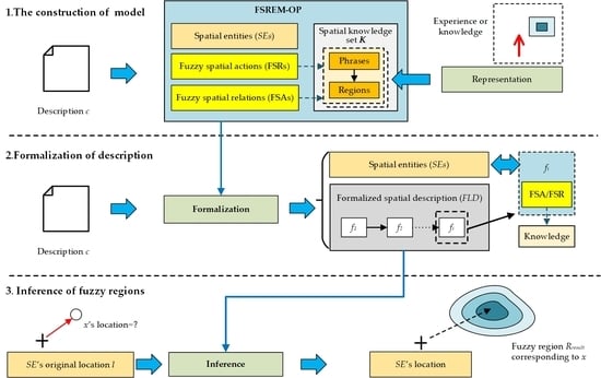
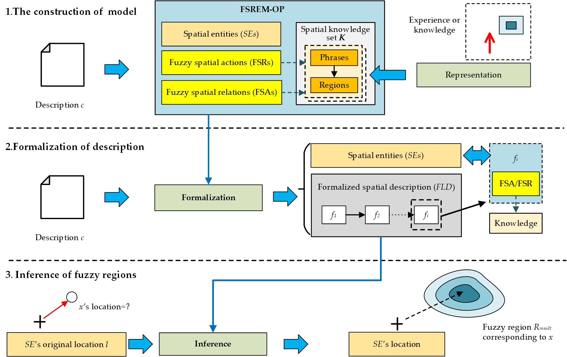
The overall process of FSREM-OP is shown in Figure 2:
Figure 2 shows that the context, experience, and knowledge related to c should be first introduced. This subjective knowledge is transformed into spatial knowledge set K. K expresses the spatial relations corresponding to c. It can be reused and support all the inference work under the same background as c (e.g., the expression of spatial relations of the same group of people). Based on the K, the whole process is divided into the following three steps:
- Model Construction: Set FSREM-OP = {SE, FSRs, FSAs} includes Spatial Entity (SE), its corresponding Fuzzy Spatial relations (FSRs) and Fuzzy Spatial actions (FSAs). In FSRs and FSAs, the process of spatial relationships is based on the content in K.
- Formalization of description: As to the description c: its content is analyzed to obtain the observer p; the instance corresponding spatial entity (SE) is built based on p, and form the formalized spatial description (FLD). FLD is a sequential structure {f1, f2, …, fn}, in which fi is an FSR or FSA. Each fi will exert an influence on the spatial position and direction of SE or output of certain spatial regions.
- Inference of fuzzy regions: Each fi in the FLD is successively executed to extract the fuzzy regions Rresult = {r1, r2, …, rn} where x is located; ri is polygon in Rresult that expresses the probability that x is in a particular area.
Through the above three steps, the spatial content of c can be extracted, and the possible regions of object x can be expressed as a set of polygon on the map to achieve fuzzy spatial region extraction.
2.3. Composition of FSREM-OP and Formalization of Description
The FSREM-OP model consists of the following three parts:
- Spatial entity (SE): SE indicates the position and direction of p on the real map, which can be expressed as SE = {lse, dse}, where lse is the spatial coordinate of p on the map. dse is the direction of p, and this direction is a clockwise angle with due north direction as angle 0.
- Fuzzy spatial relations (FSRs): FSREM-OP contains multiple spatial relations FSRs = {fsr1, fsr2, …, fsrn}, where each fsri corresponds to the knowledge in K. The function of the FSRs is to directly output a set of spatial regions according to the spatial description Phrase.
- Fuzzy spatial actions (FSAs): FSAs = {fsa1, fsa2, …, fsan}, where fsai also corresponds to the knowledge in K. Different from FSRs, the function of FSAs is to change the position and direction of SE.
With the support of the FSREM-OP model, a description c can be transformed and expressed as formalized spatial description (FLD) by sequential analysis using FSRs and FSAs. Its corresponding algorithm is represented in Algorithm 2:
| Algorithm 2: The FLDConstruction algorithm |
| Input: description c, FSREM-OP |
| Output: formalized spatial description FLD |
| Begin |
| klist = Filter and separate c into blocks according to all the phrases in K |
| FLD = ø; |
| foreach phrase in klist |
| if phrarse a description of the location |
| FLD←corresponding fsr; |
| else if phrase a description of the action |
| FLD←corresponding fsa; |
| return FLD; |
| End |
The FLD can be built by FLDConstruction algorithm. The internal FLD is composed of FSRs or FSAs. The position of x can be inferred by the sequential parsing of the FLD.
2.4. Inference of Fuzzy Regions
The inference of FLD is the process of successively analyzing each fi within the FLD to adjust the position and direction of SE or outputting regions. As for FSRs process, since FSRs represent spatial relations, a FSR only needs to output the regions in the corresponding knowledge.
For FSAs, the Regions in corresponding knowledge can bring certain fuzziness. For example, even if the same person walks for one minute, the distance traveled each time can be different. A single SE cannot express this fuzziness (one cannot be in two places at the same time), so this paper introduces the Reference CE List (listce) to express the fuzziness of different regions through the location and density of multiple CE. The specific pattern is shown in Figure 3:
In Figure 3, it is assumed that Regions is converted into the raster data of Rraster, each raster has a fuzzy membership degree; when performs random selection, the raster with a higher membership degree is more likely to be selected, whereas the opposite is less likely. In this paper, an algorithm is proposed to convert this selection idea into the selection of distances within a certain range. The corresponding algorithm is represented in Algorithm 3:
| Algorithm 3: The RandomSelect algorithm |
| Input:Rraster |
| Output: Selected raster rselected |
| Begin |
| length = 0; intervallist = ø; |
| foreach r in Rraster |
| intervallist←[length, length+r.t); |
| length = length+ r.t; |
| rand = gets a random number of [0,length); |
| postion = Find an interval that contain rand in intervallist, and obtain this inverval’s position in intervallist; |
| rselected = Rraster[postion]; |
| End |
RandomSelect algorithm is taken as the basis of the random selection mechanism. As shown in Figure 3, the FSAs inference is a process where a SE is transformed into a group of SE after the transformation of direction and position. Its corresponding algorithm is represented in Algorithm 4:
| Algorithm 4: The FSAInference algorithm |
| Input: Spatial entity SE, Region R, Number of reference CEs Nce |
| Output: list of CE listce |
| Begin |
| Rraster = transform R in to raster format; |
| listce = ø; |
| for i in 1: Nce |
| rselected = RandomSelect (Rraster); |
| SEcopy = clone a SE; |
| Adjusts the position and direction of SEcopy based on the rselected position |
| listce←SEcopy |
| return listce; |
| End |
Based on FSAInference algorithm, SE and R can be converted into a group of SE listce. In polygons of Regions, the CE density with a high membership will be higher, and vice versa. Based on this model, the expression of the fuzzy region of location and direction can be realized, and then the fuzziness of behavior can be quantified in the result. Based on the all above algorithms, the entire FLD inference process is represented in Algorithm 5:
| Algorithm 5: The FLDInference algorithm |
| Input: formalized spatial description FLD, Description c |
| Output: Result regions Rresult |
| Begin |
| SE = build initial direction and coordinates of SE based on c; |
| listce = ø; Rresult = ø; |
| listce←SE; |
| for fi in FLD |
| listtemp = ø; |
| foreach eCE in listce |
| R = CoordinateTransform(R of fi, eCE); |
| if fi is a FSR then |
| Rresult←R; listtemp←eCE; |
| else |
| listtemp←FSAInference(eCE, R, Nce); |
| listce = listtemp; |
| return Rresult; |
| End |
Since FSR and FSA are employed throughout the whole derivation of FLD inference, the CE is constantly created to describe the fuzzy action characteristics of p during the execution, and the final result is the Rresult outputted by FLD Inference.
2.5. Merger of Results
Because the result produced by FLD Inference is the list of regions, Rresult = {R1, R2, …, Rn}, where each Ri = {r1, r2, …, rn}. If the Rresult contains only one R, it means the final result of FLD Inference comes from the content of a single spatial knowledge, which can be outputted directly to the map as a result.
If the Rresult contains multiple regions, an overlapping of these regions will occur. The final processed output is illustrated in Figure 4:
The steps to combine the contents of Rresult into the final output are:
Firstly, all Ri in Rresult are combined based on coordinate positions. As shown from the result of the combination, each overlapping polygon is separately represented to form Runion = {r1, r2, …, rn} according to the different overlapping. For ri, its membership value is equal to the sum of the membership of all regions forming this region. At this point, if the number of polygons is too large, there will be too many fragmented polygons in Runion, to be conducive to people’s understanding of the final output result. Therefore, we need to perform transformation. Based on the Runion corresponding area we create Mcell = {r1,r2, …, rn}. In the area corresponding to Mcell, the whole area is divided into polygons ri which a width×width sized square; the membership value of ri equals to the highest membership value of polygons in Runion that intersects with it.
In the Runion, too many overlapped regions will lead to ri’s membership value higher than 1, which is not conducive to truly showing and comparing the membership of different regions. Therefore, this method also remaps the weights in ri.
The membership values are remapped from 0.1 to 1.0. After that, a filter parameter, Vfilter, is specified to filter out all the cells that are smaller than the parameter to get the final merging result.
3. Experiment
3.1. Algorithm Implementation and Construction of Spatial Knowledge Set
The FSREM-OP method in this paper was implemented by Python 3.6, and the geographic information access part was implemented by Arcpy extension package of ArcGIS Pro. The geographic environment in which the algorithm operates is a project based on ArcGIS Pro. The output of FSREM-OP adopted the layer-based output mechanism; the position and direction of SEs were output to the point-based layer, and all Regions were output to the polygon-based layer. All algorithms were run on Intel i9 9900K/64GB memory PC to obtain the results.
To create the knowledge set K more conveniently, an interactive mapping program was written based on C# 4.0. This program receives user input to draw polygons and specifies the weight value of each polygon and then stores them as spatial knowledge. Through investigation and analysis, a spatial knowledge set was constructed, which includes the information of students with average height and physical condition from Changchun Institute of Technology (CCIT). CCIT is located in Changchun City, Jilin Province, Northeast China. It is a higher education institution with more than 10,000 students. This knowledge shows the cognition of spatial attributes and spatial relations by the students of CCIT as observers. We created six groups of phrases: adjacent, not far, slightly far, walking a few paces, walking for one to five minutes, and real ground objects corresponding to observer. Although these phrases are vague, the distance and spatial relationship in these phrases are obviously different. We randomly selected 50 students; they drew polygons to describe their subjective views on these phrases, and based on union of the polygons, we obtained specific content, as shown in Table 1:
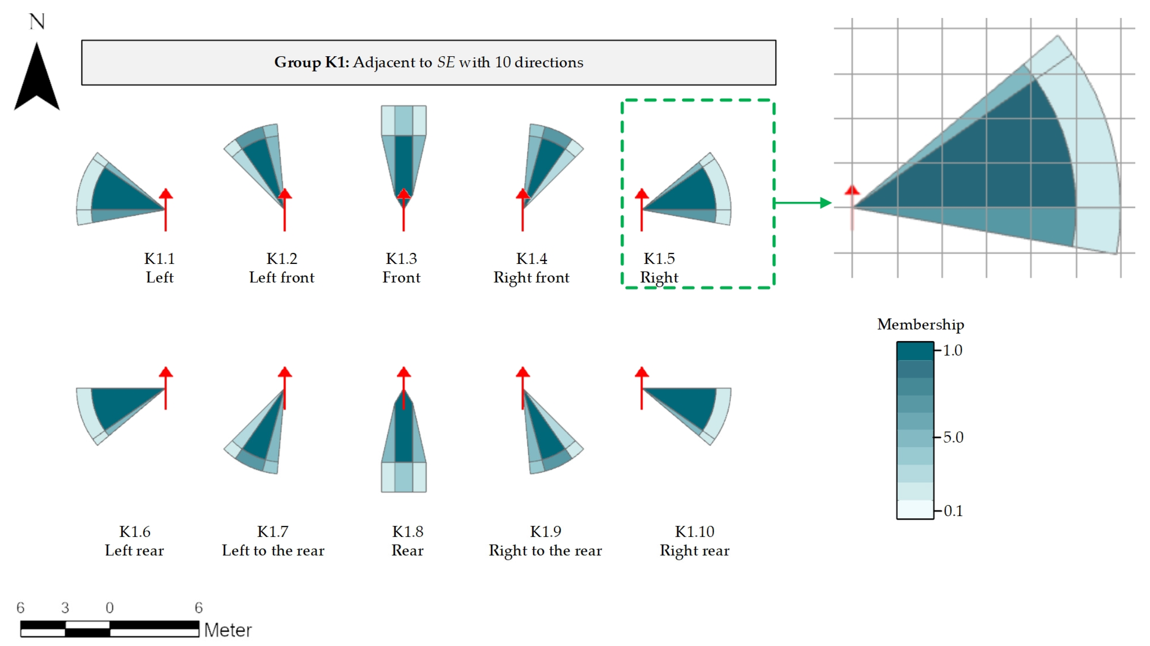
As shown in Table 1, this paper constructs a total of six groups of spatial location knowledge to form the knowledge set K, which defines the spatial knowledge adopted by the observers who are students from CCIT. In the “Phrase Description and its knowledge” column of Table 1; not only is each group of phrase described, but also the distance relationship between the phrase and the observer is quantitatively described. These quantitative values correspond to the union of results of polygons drawn by students. Taking the K1 group as an example, the spatial display effect of all knowledge in this group is shown in Figure 5:
In Figure 5, the red arrow is SE’s default direction (due north direction). Each spatial knowledge is composed of {Phrases, Regions}, in which Phrases correspond to the corresponding spatial description. Regions are composed of multiple polygons. Each polygon corresponds to membership value. Different from the traditional method, the spatial location and regional knowledge in this paper are the expressions based on the subjective viewpoint of the observers. For the expression of “Right” (the green dotted line focused), it can be seen that “left” is not the strict result of the rotation of 90° to SE, nor is it a uniformed distribution function of 45° to 135° in the traditional way. It is a combination of multiple spatial regions within a certain range. The membership between 60° and 90° is higher, but after 90° the region occupied is a smaller area with a smaller membership. These Regions correspond to an area that is more comfortable for the observers to “look” at an object on the right. Statistically speaking, the majority of students in our school are “right-handed”, so K1 tends to reflect the knowledge of “right-handed” students. Although “right-handed” and “left-handed” students are consistent in ability of spatial direction/distance representation, there may be slight differences in detail between them. Different group divisions will produce different knowledge structures. In further research, we will consider subdividing the groups and construction knowledge set with more detailed parameters. Based on the knowledge set K, a vague description c from our students can be translated into quantitative and qualitative polygons, and can be represented in GIS.
3.2. Spatial Regional Inference Tested in Real Geographical Scenarios
To test the effectiveness of the FSREM-OP method, this paper introduces the knowledge shown in Table 1 into the space of CCIT. The corresponding space on the campus of CCIT is shown in Figure 6:
In Figure 6a is the space scope corresponding to CCIT. Figure 6b is an object x inside a square. For this object, its location needs to be inferenced by the following descriptions:
(a) A student is positioned at p1 towards p2 and sees an object x in his right front.
(b) The position of a student is at p3 towards p4 and object x is in his left front.
(c) A student faces p6 at p5 and finds that object x is not far ahead of him.
(d) A student faces due north at p7, then he turns to the right.
(e) A student walks from p8 to p9 for a few seconds and finds object x on his right.
FSREM-OP method was used to conduct spatial inference on the above descriptions. FSR and FSA were used to analyze the spatial relationship. The FLD was obtained as shown in Table 2.
As Table 2 shows, different spatial knowledge was used to infer the spatial regions of object x from 1 to 5. Based on this knowledge, the inferred results are displayed on the map, as shown in Figure 7:
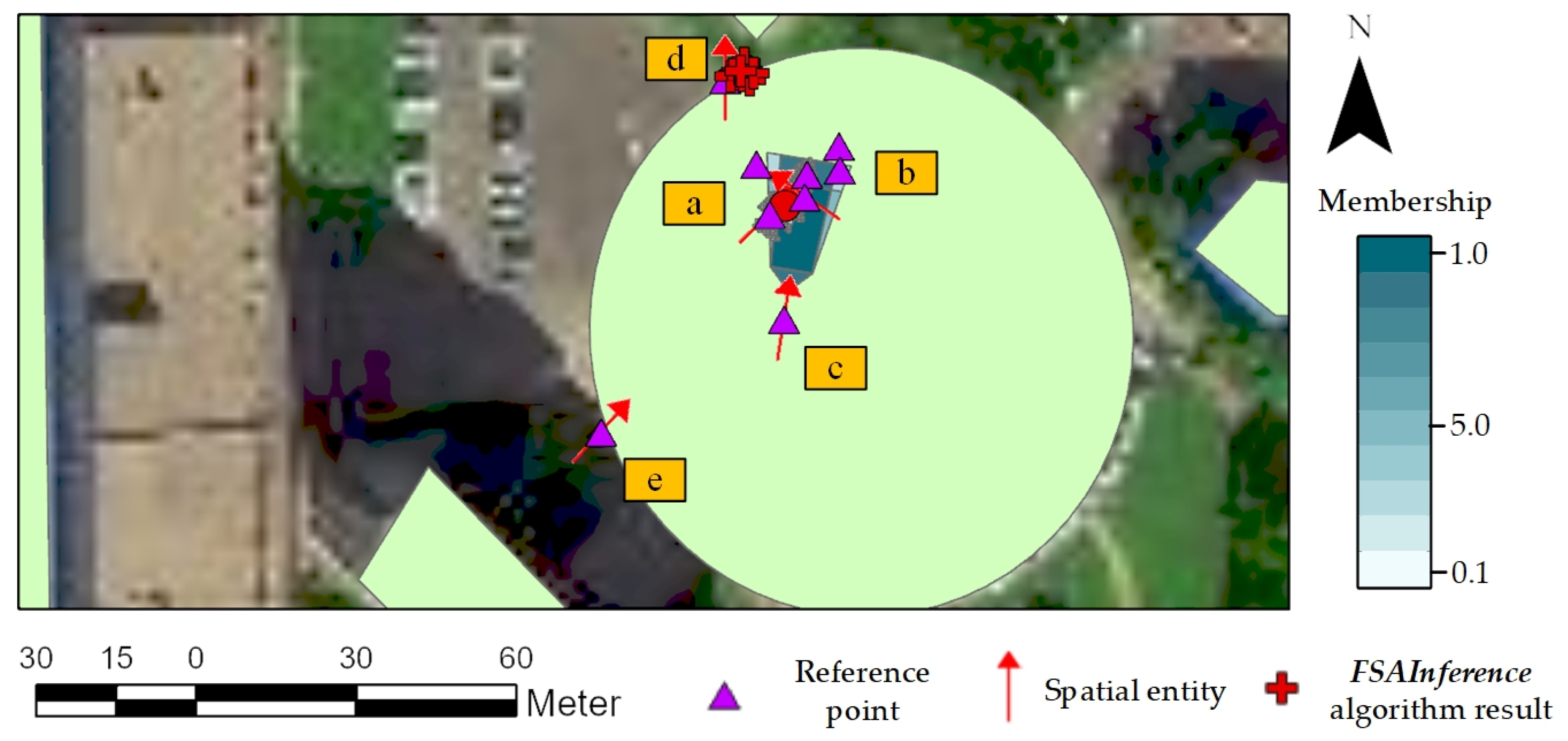
As Figure 7 shows, each description from (a) to (e) can obtain the corresponding Regions. These regions have different directions and polygons. Figure 8 shows the detail result of each description, respectively:
In Figure 8, the red circle is marked as the position of object x, the red arrow corresponds to the position and direction of SE, and the purple triangle is the reference point.
3.3. Discussion of the Spatial Regional Inference
In Figure 8a,b, it can be seen that FSREM-OP shows the space range corresponding to the descriptions (a) and (b). Object x is located in the region with high member value corresponding to the description (a) and (b); it shows that FSREM-OP and K can obtain the corresponding region of fuzzy description for the adjacent objects. For Figure 8c, because the description of “nearer” is larger in spatial range, the spatial range of K2.3 within spatial knowledge is significantly larger than that of K1 group. As a result, object x is in the region with a higher weight value in this larger region.
The operation in Figure 8d corresponds to the FSA that is based on knowledge K1.5. In the figure, the red sign of “+” corresponds to the running result of the FSAInference algorithm, whose parameter Nce is set as 10. It can be seen that the density of CEs obtained in the region of a high weight value is larger, while the density is smaller or to none in the region of low weight value. These CEs listce can be used as references for the CE steering. The yellow arrows in Figure 8d indicate the possible SE directions.
Figure 8e corresponds to the description e, which contains one FSA and one FSR and requires running multiple steps to get the result. First, FSA introduces knowledge K4.1 and uses FSAInference algorithm which Nce set to 10 to generate reference listce. Secondly, CEs in listce uses FSR to introduce knowledge K1.1 to product fuzzy spatial region. For listce, it can be seen that the more CEs appear in the region with higher weight value, the more knowledge K1.1 corresponding regions are produced on the map. Further, the overlap degree of the corresponding direction is also higher. Meanwhile, in the region with lower member value, CEs appear less and the overlap degree is lower. All CEs in listce merge result Runion can be seen in the last image of Figure 8e, the value of the parameter Vfilter is set at 0.0001 (filtering only cells with a member value of 0); in the result, the grid size of is set by 0.5 m × 0.5 m, and the weight of the corresponding grid is also high for regions with high overlap. It can be seen that object x is in the region with a high member value. The number of corresponding grids is 424, and the corresponding area is 424 × 0.25 = 106 m2. The low-probability cells can be filtered out by increasing the value of Vfilter to get more precise regions. However, as the distribution direction and quantity of the final results are affected by the characteristics of FSA and FSR, the simple improvement of Vfilter may not necessarily make the final results contain object x. From Figure 8f, it can be seen that the typical direction of the high-probability grids is consistent with the SE distribution direction in the original FSA. The continuous improvement of the value of Vfilter can reduce the scope of the obtained area. When Vfilter equals 0.6, the corresponding area of 42 areas is 42 × 0.25 = 10.5m2. However, when Vfilter equals 0.8, object x falls outside the result area.
3.4. Refining Regions by Merging Multiple Descriptions’ Results
As can be seen from the results in Section 3.2, for the location description of object x after the action FSA is performed, the area of inference results will be larger, which makes the regions of x highly vague. This vagueness is caused by the fuzziness of description itself (uncertainty of position, direction, and distance), which cannot be reduced simply by improving the method itself. It is also not appropriate to simply assume that object x must be in the region of highest weight value from just one description. For example, in Figure 8f, when Vfilter equals 0.8, object x falls out of the result region.
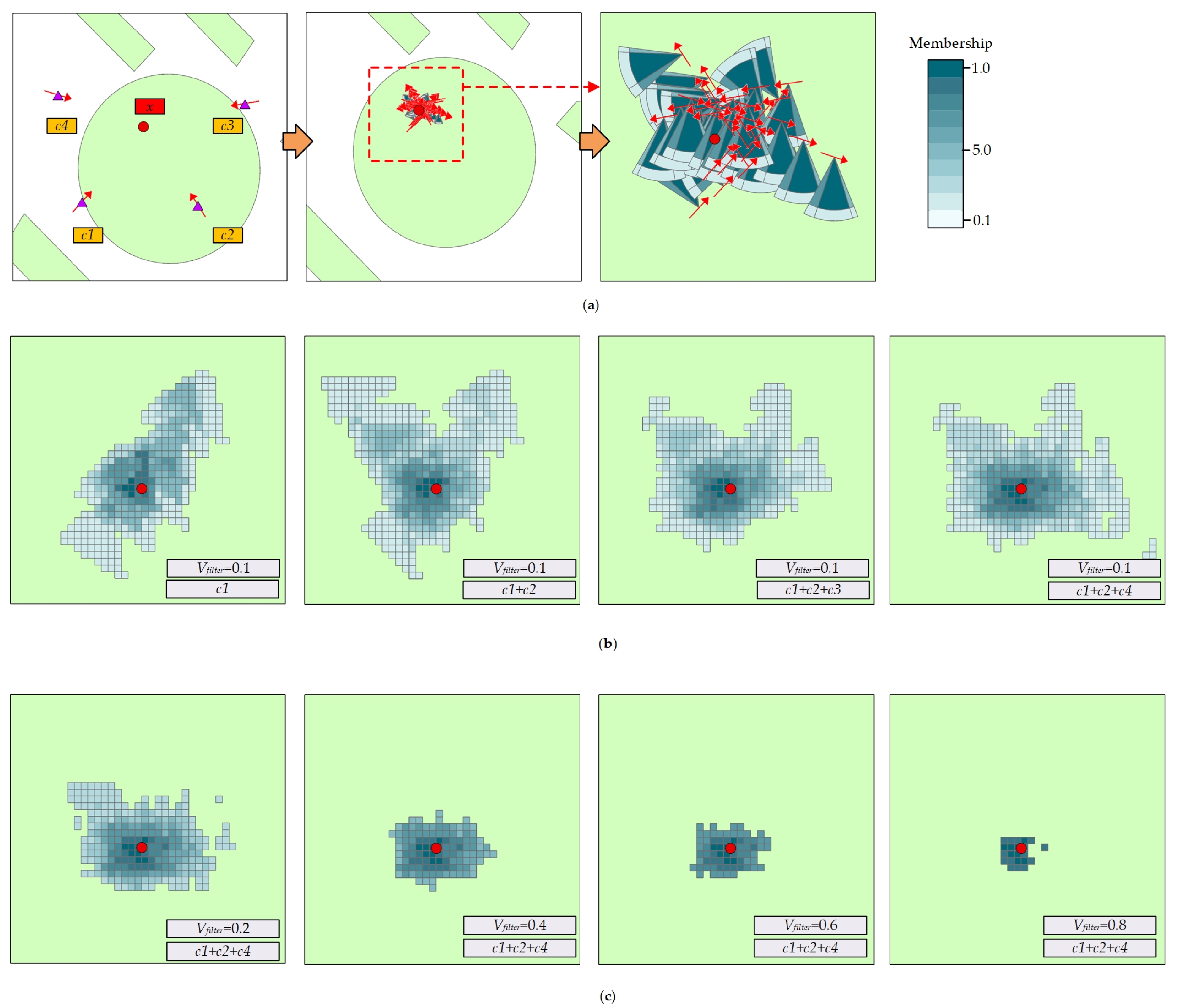
To reduce the range and fuzziness of the predicted location of object x and improve the accuracy of location determination, multiple multi-directional observation descriptions can be introduced (for example, multiple witnesses have seen object x at a certain location) and the method of result merging can be adopted. As shown in Figure 9, on the basis of describing (e), additional three directions can be introduced to describe and infer the results:
3.5. Discussion of the Merging of the Multiple Description Results
Figure 9a shows four added descriptions. c1 is the same as the description (e) in Section 3.2. c2 and c3 change directions. c4 not only changes direction but also object x at SE’s right side. The four descriptions will derive 40 groups of Regions, and each region contains six polygons, 240 polygons in total. Figure 9b shows that the four descriptions’ Rresult are gradually merged into Runion. It can be seen that with more Rresult, the regional weight division around object X gradually turns from certain direction into a circle. Object x is in the highest region of the weight value. With the increase of the distance from it, this weight value gradually decreases. Figure 9c shows that when more descriptions are added, the value of Vfilter is increased and the result area is obviously gradually reduced around object x. When Vfilter equals 0.8, the result only contains 22 cells with a size of 22 × 0.25 = 5.5 m2. It can be seen from this process that in inferring the objects of unknown locations, descriptions (or eyewitness description) introduced in multiple directions can be merged with the results in multiple directions to obtain more accurate positions.
4. Conclusions
The spatial location descriptions of objects in eyewitness records, travel notes and historical documents are often observer-centered, vague and subjective. Traditional methods of extracting location by the name or extracting topological relationship between objects can hardly process such descriptions. To extract spatial information from these descriptions effectively, this paper proposes the FSREM-OP method. The FSREM-OP can handle the regions and spatial information in the observer-centered descriptions, and represent corresponding vague locations in the GIS. The novel features of FSREM-OP are listed as follows:
- Spatial representation of the subjective viewpoints: FSREM-OP can transform subjective viewpoints to spatial regions. FSREM-OP introduces the form of {Phrase, Regions} to express spatial knowledge, and transforms the experiments or viewpoints of a group of observers on spatial relations into a group of polygons. These polygons can establish the relationship between vague spatial concepts and the qualitative/quantitative spatial data, so as to realize the expression of vague observer-center spatial location descriptions in the GIS.
- Vague spatial relation and region inference: FSREM-OP can progressively infer spatial relations and regions. For a description, FSREM-OP builds an FLD by splitting descriptions so that the original text description is transformed into a list of spatial relations and actions. For this list, FSR and FSA are used to process spatial information, respectively, in order to produce the merged spatial regions and complete the inference process. Through this process, the behavior and knowledge of the observer in descriptions can be gradually added to the final fuzzy region result.
In the experiment, the space knowledge based on specific groups was built and its inference capability was verified in a real place. The results show that FSREM-OP can transform the object’s vague location description into fuzzy spatial regions and present it to the GIS in the form of polygons with the weight value. This capability can establish the relationship between the spatial relationship of geographic information and the object’s fuzzy location description. As a result, FSREM-OP can be used as a bridge between vague location descriptions and quantitative/qualitative geographic information. It provides the data basis for a variety of applications that require objects’ spatial locations as evidence.
Author Contributions
Conceptualization, Jun Xu; data curation, Xin Pan; methodology, Jun Xu; supervision, Jun Xu; visualization, Xin Pan; writing—original draft, Xin Pan. All authors have read and agreed to the published version of the manuscript.
Funding
This research was jointly supported by the National Natural Science Foundation of China (41971193; 41871236) and the Natural Science Foundation of Jilin Province (20200403174SF; 20180622006JC; 20180101020JC; 20200403187SF).
Conflicts of Interest
The authors declare no conflict of interest.
References
- Liu, Y.; Liu, X.; Gao, S.; Gong, L.; Kang, C.; Zhi, Y.; Chi, G.; Shi, L. Social sensing: A new approach to understanding our socioeconomic environments. Ann. Assoc. Am. Geogr. 2015, 105, 512–530. [Google Scholar] [CrossRef]
- Zhuo, L.; Shi, Q.; Zhang, C.; Li, Q.; Tao, H. Identifying Building Functions from the Spatiotemporal Population Density and the Interactions of People among Buildings. ISPRS Int. J. Geo-Inf. 2019, 8, 247. [Google Scholar] [CrossRef] [Green Version]
- Goodchild, M.; Egenhofer, M.J.; Fegeas, R.; Kottman, C. Interoperating Geographic Information Systems; Kluwer Academic Publishers: Boston, MA, USA, 1999. [Google Scholar]
- Couclelis, H. Towards an Operational Typology of Geographic Entities with Ill-defined. In Geographic Objects with Indeterminate Boundaries; Taylor & Francis: London, UK, 1996; Volume 2, p. 45. [Google Scholar]
- Burrough, P.A. Natural Objects with Indeterminate Boundaries. In Geographic Objects with Indeterminate Boundaries; Taylor & Francis: London, UK, 1996; Volume 2, p. 3. [Google Scholar]
- Duckham, M. Keynote paper: Representation of the natural environment. In Representing, Modeling, and Visualizing the Natural Environment; CRC Press: Boca Raton, FL, USA, 2008; pp. 27–36. [Google Scholar]
- Zhang, J.; Goodchild, M.F. Uncertainty in Geographical Information; Taylor and Francis: New York, NY, USA, 2002. [Google Scholar]
- Fisher, P.; Cheng, T.; Wood, J. Higher order vagueness in geographical information: Empirical geographical population of type n fuzzy sets. Geoinformatica 2007, 11, 311–330. [Google Scholar] [CrossRef]
- Bittner, T. Vagueness and the trade-off between the classification and delineation of geographic regions–an ontological analysis. Int. J. Geogr. Inf. Sci. 2011, 25, 825–850. [Google Scholar] [CrossRef]
- Schmidt, J.; Hewitt, A. Fuzzy land element classification from DTMs based on geometry and terrain position. Geoderma 2004, 121, 243–256. [Google Scholar] [CrossRef]
- Ahlqvist, O.; Keukelaar, J.; Oukbir, K. Rough and fuzzy geographical data integration. Int. J. Geogr. Inf. Sci. 2003, 17, 223–234. [Google Scholar] [CrossRef]
- Burrough, P.A.; van Gaans, P.F.; MacMillan, R. High-resolution landform classification using fuzzy k-means. Fuzzy Sets Syst. 2000, 113, 37–52. [Google Scholar] [CrossRef]
- Arrell, K.; Fisher, P.F.; Tate, N.; Bastin, L. A fuzzy c-means classification of elevation derivatives to extract the morphometric classification of landforms in Snowdonia, Wales. Comput. Geosci. 2007, 33, 1366–1381. [Google Scholar] [CrossRef]
- Qin, C.-Z.; Zhu, A.-X.; Shi, X.; Li, B.-L.; Pei, T.; Zhou, C.-H. Quantification of spatial gradation of slope positions. Geomorphology 2009, 110, 152–161. [Google Scholar] [CrossRef]
- Brown, D.G. Classification and boundary vagueness in mapping presettlement forest types. Int. J. Geogr. Inf. Sci. 1998, 12, 105–129. [Google Scholar] [CrossRef]
- Wang, D.; Laffan, S.W.; Liu, Y.; Wu, L. Morphometric characterisation of landform from DEMs. Int. J. Geogr. Inf. Sci. 2010, 24, 305–326. [Google Scholar] [CrossRef] [Green Version]
- Rocchini, D.; Foody, G.M.; Nagendra, H.; Ricotta, C.; Anand, M.; He, K.S.; Amici, V.; Kleinschmit, B.; Förster, M.; Schmidtlein, S. Uncertainty in ecosystem mapping by remote sensing. Comput. Geosci. 2013, 50, 128–135. [Google Scholar] [CrossRef]
- Gorini, M.A.V.; Mota, G.L.A. Dealing with double vagueness in DEM morphometric analysis. Int. J. Geogr. Inf. Sci. 2016, 30, 1644–1666. [Google Scholar] [CrossRef]
- Jadidi, A.; Mostafavi, M.A.; Bédard, Y.; Shahriari, K. Spatial representation of coastal risk: A fuzzy approach to deal with uncertainty. ISPRS Int. J. Geo-Inf. 2014, 3, 1077–1100. [Google Scholar] [CrossRef]
- Guilbert, E.; Moulin, B. Towards a common framework for the identification of landforms on terrain models. ISPRS Int. J. Geo-Inf. 2017, 6, 12. [Google Scholar] [CrossRef]
- Liu, Y.; Yuan, Y.; Gao, S. Modeling the Vagueness of Areal Geographic Objects: A Categorization System. ISPRS Int. J. Geo-Inf. 2019, 8, 306. [Google Scholar] [CrossRef] [Green Version]
- Abdelkader, A.; Hand, E.; Samet, H. Brands in NewsStand: Spatio-temporal browsing of business news. In Proceedings of the 23rd SIGSPATIAL International Conference on Advances in Geographic Information Systems, Seattle, WA, USA, 3–6 November 2015; pp. 1–4. [Google Scholar]
- Adams, B.; McKenzie, G.; Gahegan, M. Frankenplace: Interactive thematic mapping for ad hoc exploratory search. In Proceedings of the 24th International Conference on World Wide Web, Florence, Italy, 18–22 May 2015; pp. 12–22. [Google Scholar]
- Li, T.J.-J.; Sen, S.; Hecht, B. Leveraging advances in natural language processing to better understand Tobler’s first law of geography. In Proceedings of the 22Nd ACM SIGSPATIAL International Conference on Advances in Geographic Information Systems, Dallas, TX, USA, 4–7 November 2014; pp. 513–516. [Google Scholar]
- VoPham, T.; Hart, J.E.; Laden, F.; Chiang, Y.-Y. Emerging trends in geospatial artificial intelligence (geoAI): Potential applications for environmental epidemiology. Environ. Health 2018, 17, 40. [Google Scholar] [CrossRef]
- Andrea Rodriguez, M.; Egenhofer, M.J. Comparing geospatial entity classes: An asymmetric and context-dependent similarity measure. Int. J. Geogr. Inf. Sci. 2004, 18, 229–256. [Google Scholar] [CrossRef]
- Yi, S.; Huang, B.; Chan, W.T. XML application schema matching using similarity measure and relaxation labeling. Inf. Sci. 2005, 169, 27–46. [Google Scholar] [CrossRef]
- Nedas, K.A.; Egenhofer, M.J. Spatial-scene similarity queries. Trans. Gis 2008, 12, 661–681. [Google Scholar] [CrossRef]
- Janowicz, K.; Raubal, M.; Kuhn, W. The semantics of similarity in geographic information retrieval. J. Spat. Inf. Sci. 2011, 2011, 29–57. [Google Scholar] [CrossRef]
- Kim, J.; Vasardani, M.; Winter, S. Similarity matching for integrating spatial information extracted from place descriptions. Int. J. Geogr. Inf. Sci. 2017, 31, 56–80. [Google Scholar] [CrossRef]
- Blaschke, T.; Merschdorf, H. Geographic information science as a multidisciplinary and multiparadigmatic field. Cartogr. Geogr. Inf. Sci. 2014, 41, 196–213. [Google Scholar] [CrossRef] [Green Version]
- Blaschke, T.; Merschdorf, H.; Cabrera-Barona, P.; Gao, S.; Papadakis, E.; Kovacs-Györi, A. Place versus space: From points, lines and polygons in gis to place-based representations reflecting language and culture. ISPRS Int. J. Geo-Inf. 2018, 7, 452. [Google Scholar] [CrossRef] [Green Version]
- MacEachren, A.M. Leveraging big (geo) data with (geo) visual analytics: Place as the next frontier. In Spatial Data Handling in Big Data Era; Springer: Berlin/Heidelberg, Germany, 2017; pp. 139–155. [Google Scholar]
- Vasardani, M.; Winter, S.; Richter, K.-F. Locating place names from place descriptions. Int. J. Geogr. Inf. Sci. 2013, 27, 2509–2532. [Google Scholar] [CrossRef]
- Gao, S.; Janowicz, K.; Montello, D.R.; Hu, Y.; Yang, J.-A.; McKenzie, G.; Ju, Y.; Gong, L.; Adams, B.; Yan, B. A data-synthesis-driven method for detecting and extracting vague cognitive regions. Int. J. Geogr. Inf. Sci. 2017, 31, 1245–1271. [Google Scholar] [CrossRef]
- Wu, X.; Wang, J.; Shi, L.; Gao, Y.; Liu, Y. A fuzzy formal concept analysis-based approach to uncovering spatial hierarchies among vague places extracted from user-generated data. Int. J. Geogr. Inf. Sci. 2019, 33, 991–1016. [Google Scholar] [CrossRef]
- Liu, X.; Kar, B.; Montiel Ishino, F.A.; Zhang, C.; Williams, F. Assessing the Reliability of Relevant Tweets and Validation Using Manual and Automatic Approaches for Flood Risk Communication. ISPRS Int. J. Geo-Inf. 2020, 9, 532. [Google Scholar] [CrossRef]
- Shi, W.; Liu, K. A fuzzy topology for computing the interior, boundary, and exterior of spatial objects quantitatively in GIS. Comput. Geosci. 2007, 33, 898–915. [Google Scholar] [CrossRef]
- Winter, S. Uncertain topological relations between imprecise regions. Int. J. Geogr. Inf. Sci. 2000, 14, 411–430. [Google Scholar] [CrossRef]
- Tang, X.; Kainz, W.; Fang, Y. Reasoning about changes of land covers with fuzzy settings. Int. J. Remote Sens. 2005, 26, 3025–3046. [Google Scholar] [CrossRef]
- Klajnšek, G.; Žalik, B. Merging polygons with uncertain boundaries. Comput. Geosci. 2005, 31, 353–359. [Google Scholar] [CrossRef]
- Liu, K.; Shi, W. Computing the fuzzy topological relations of spatial objects based on induced fuzzy topology. Int. J. Geogr. Inf. Sci. 2006, 20, 857–883. [Google Scholar] [CrossRef]
- Zhang, Z.; Demšar, U.; Wang, S.; Virrantaus, K. A spatial fuzzy influence diagram for modelling spatial objects’ dependencies: A case study on tree-related electric outages. Int. J. Geogr. Inf. Sci. 2018, 32, 349–366. [Google Scholar] [CrossRef]
- Dilo, A.; De By, R.A.; Stein, A. A system of types and operators for handling vague spatial objects. Int. J. Geogr. Inf. Sci. 2007, 21, 397–426. [Google Scholar] [CrossRef]
- Majic, I.; Naghizade, E.; Winter, S.; Tomko, M. RIM: A ray intersection model for the analysis of the between relationship of spatial objects in a 2D plane. Int. J. Geogr. Inf. Sci. 2020, 1–26. [Google Scholar] [CrossRef]
Figure 1.
The definition and coordinate transformation of local regions Rlocal and global regions Rglobal.
Figure 1.
The definition and coordinate transformation of local regions Rlocal and global regions Rglobal.
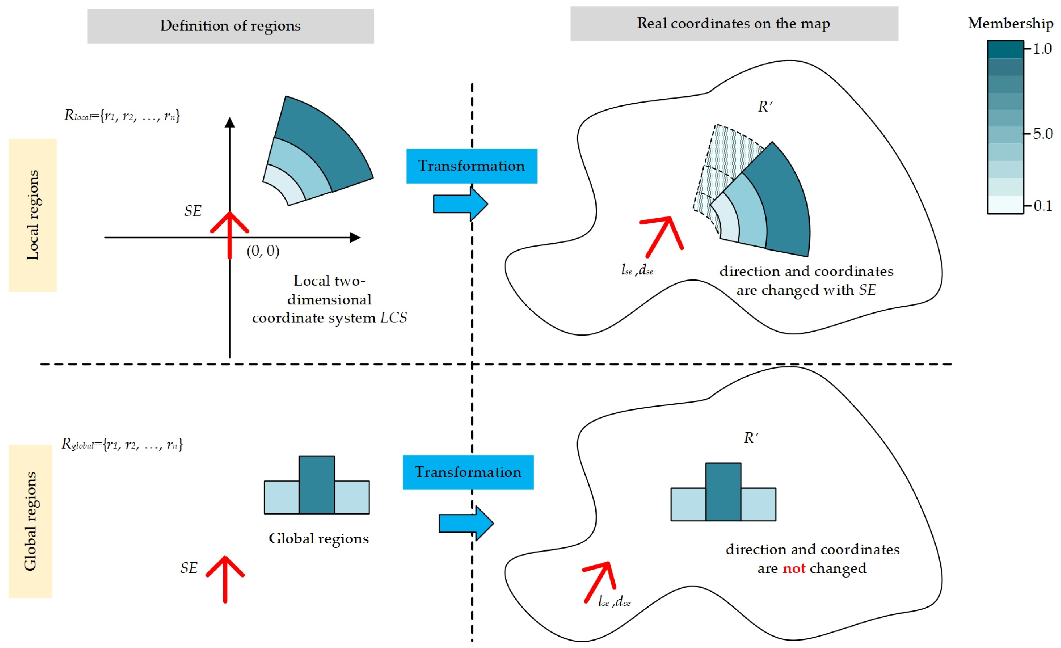
Figure 2.
The overall process of FSREM-OP.
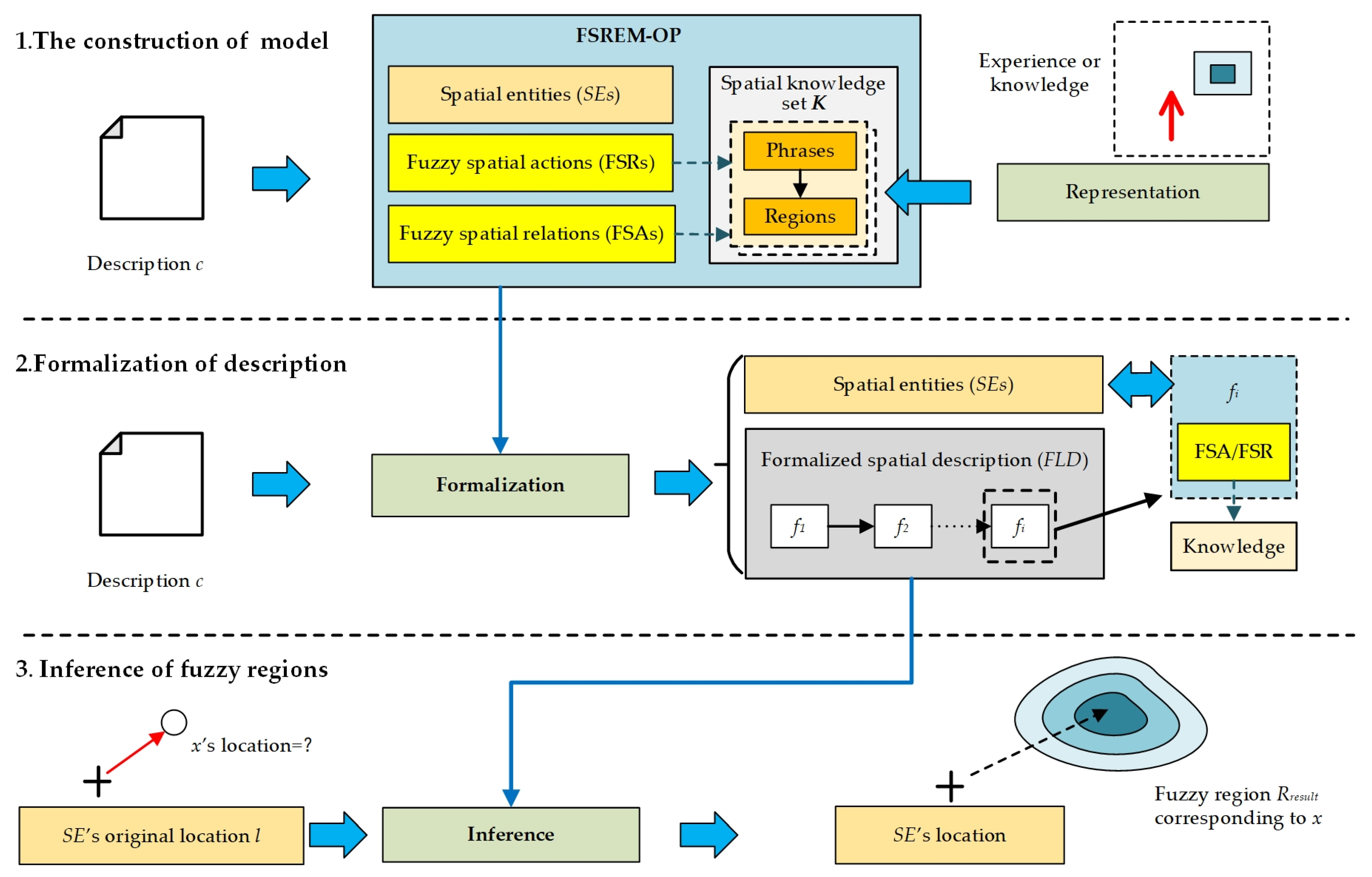
Figure 3.
Express the fuzziness of different regions by listce.
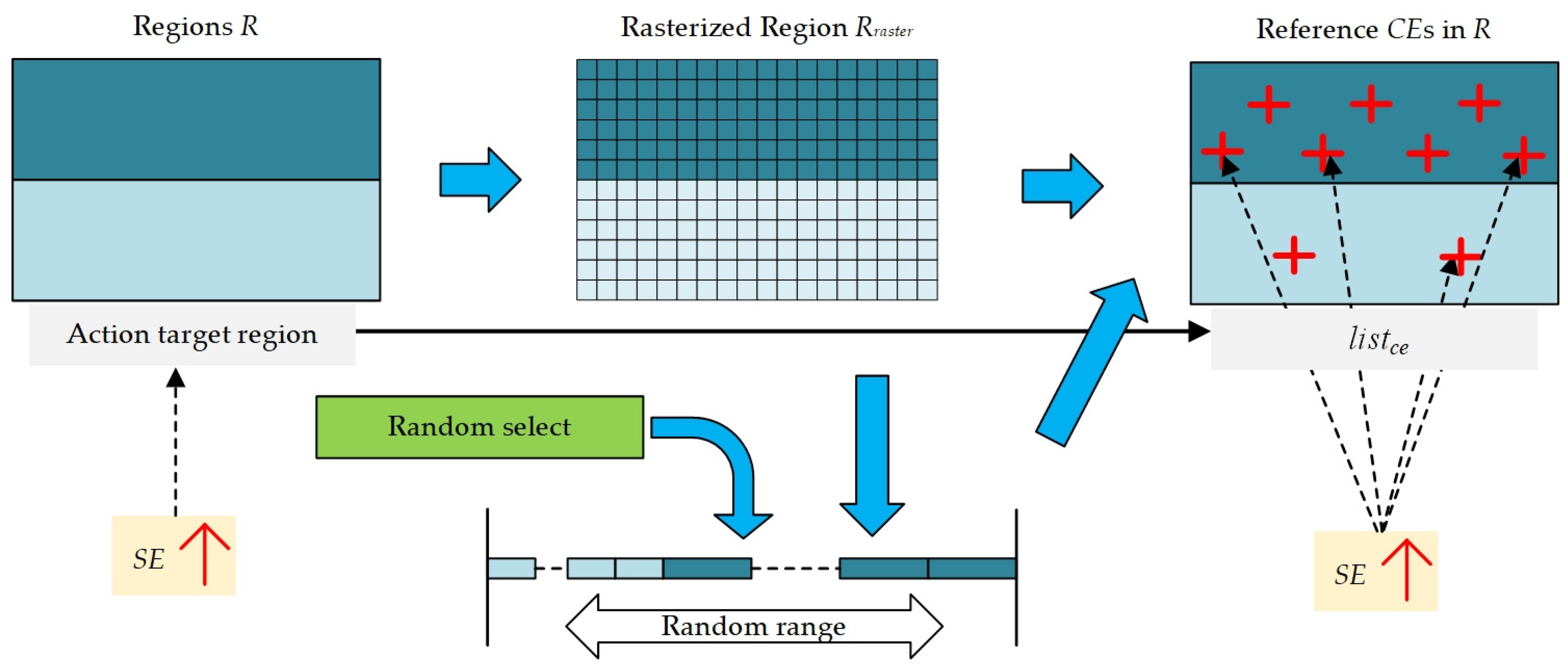
Figure 4.
Merging process of the results.
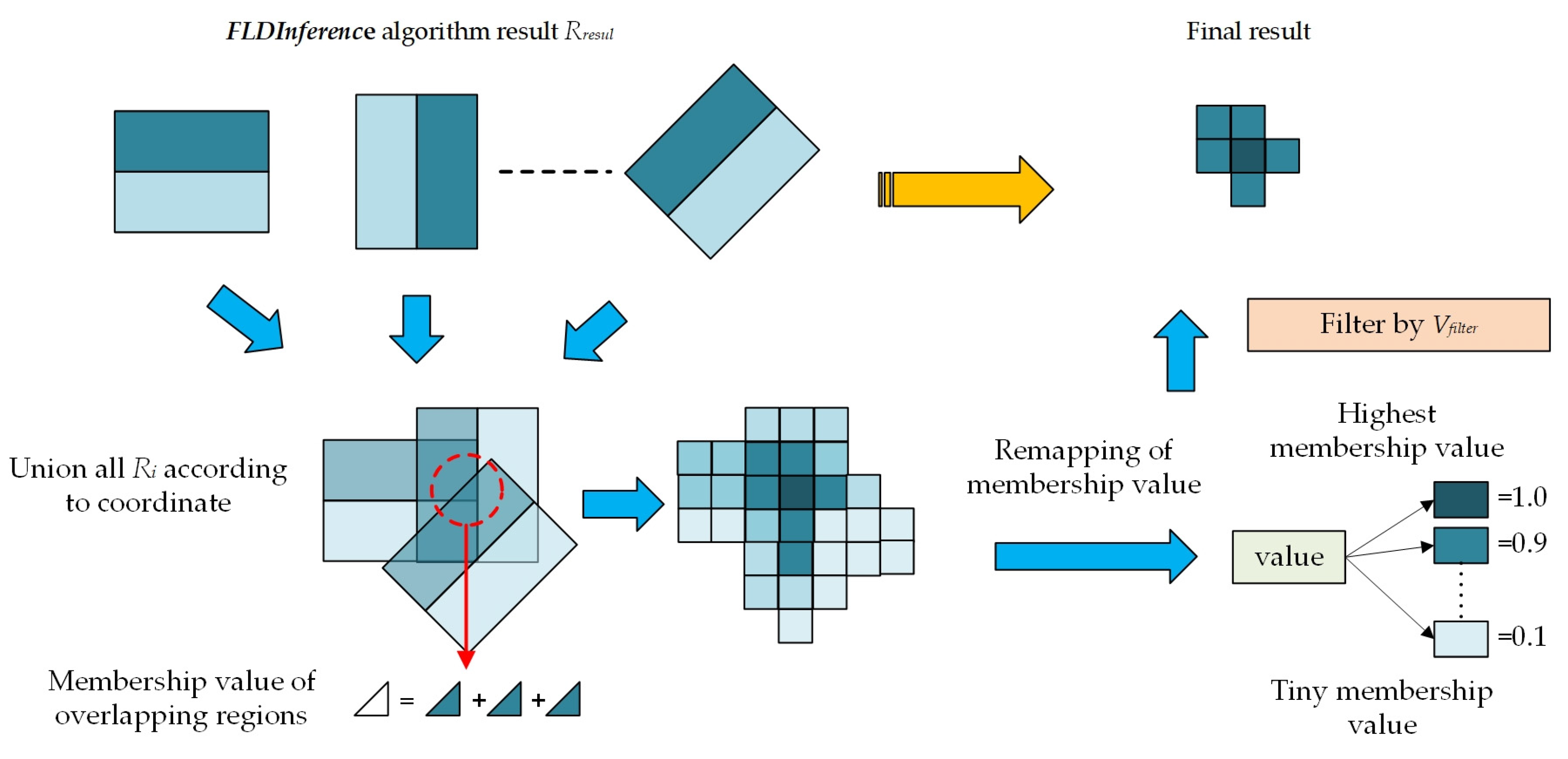
Figure 5.
The knowledge of group K1.

Figure 6.
Study area and target; (a) study area; (b) target object x and corresponding point.

Figure 7.
The results of FSREM-OP on description a to e.

Figure 8.
The amplification result of descriptions: (a) result of description a; (b) result of description b; (c) description c; (d) action result of description d; (e) detail result of description e; (f) the influence of Vfilter.
Figure 8.
The amplification result of descriptions: (a) result of description a; (b) result of description b; (c) description c; (d) action result of description d; (e) detail result of description e; (f) the influence of Vfilter.
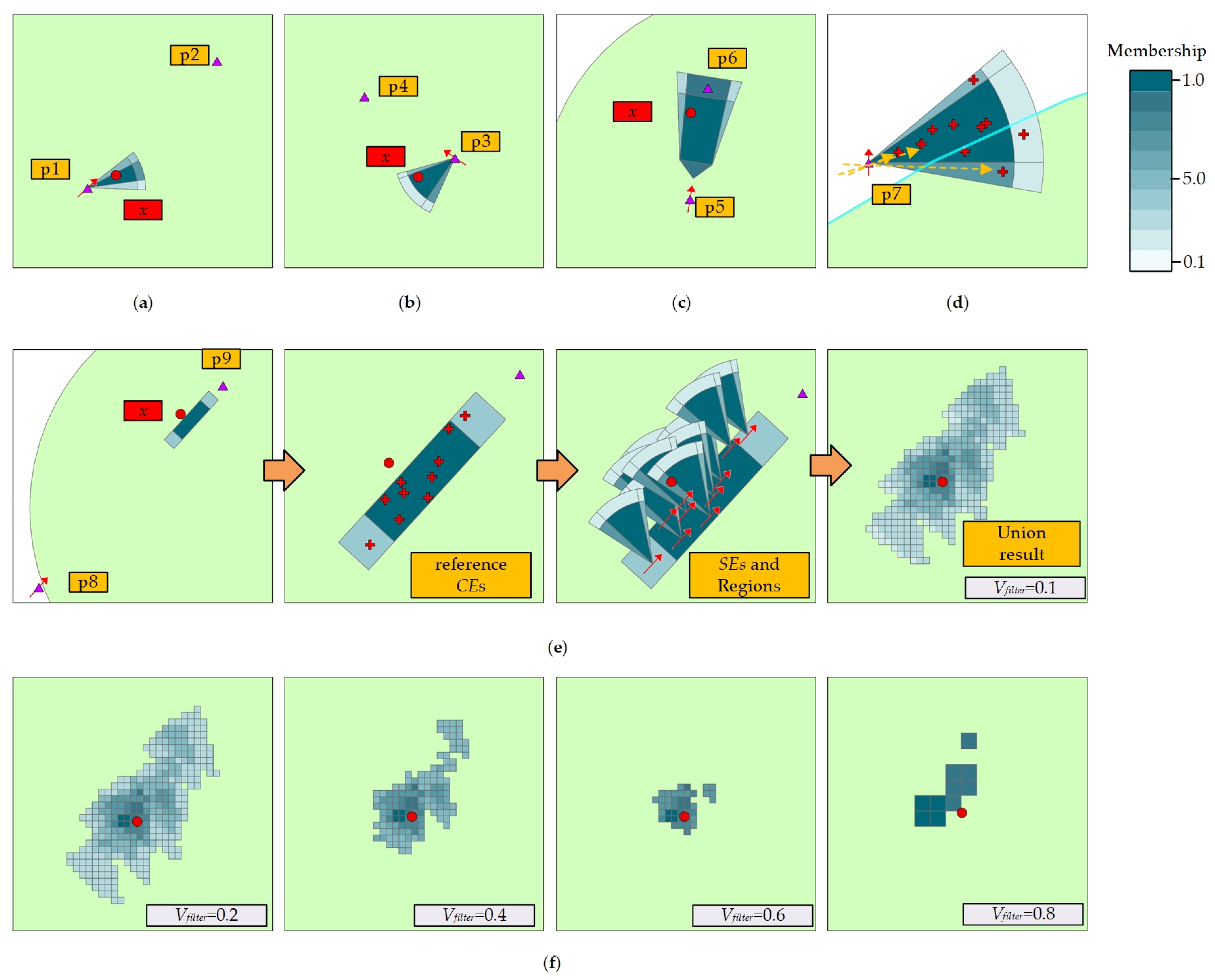
Figure 9.
Results after introducing multiple descriptions: (a) Four added descriptions and result; (b) four descriptions’ Rresult are gradually merged into Runion; (c) the influence of Vfilter.
Figure 9.
Results after introducing multiple descriptions: (a) Four added descriptions and result; (b) four descriptions’ Rresult are gradually merged into Runion; (c) the influence of Vfilter.


Table 1.
Observer’s spatial knowledge set K.
| Group No. | Phrase Description and Its Knowledge | Content and Number |
|---|---|---|
| K1 | The spatial region is adjacent to the observer, within 0 to 6 m with the observer-centered. | The knowledge ID from K1.1 to K1.10 represent the observer-centered left, left front, front, right front, right, right rear, right to the rear, back, and left to the rear and left rear. |
| K2 | Spatial region is not far from the observer, within 5 to 30 m. | The knowledge ID from K2.1 to K2.10 represent the left, left front, front, right front, right, right rear, right to the rear, back, left to the rear and left rear with a certain distance to the observer. |
| K3 | Spatial region that is slightly far from the observer within 25 to 150 m. | The knowledge ID from K3.1 to K3.10 represent the left, left front, front, right front, right, right rear, right to the rear, back, left to the rear and left rear with a far distance to the observer. |
| K4 | Walking a few paces ahead for a few seconds. Within 1–3 m of the observer. | The knowledge ID is K4.1, within the scope of an area in front of the observer. |
| K5 | Walking for one minute, two to five minutes. The distance to observer is [μ-σ, μ+σ], μ is the average walking speed, σ is the standard deviation of the speed of walking. | The knowledge ID from K5.1 to K5.5. |
| K6 | Rglobal type area built based on real ground objects. | According to the corresponding ground object. |
Table 2.
FSRs and FSRs in FLD.
| Description | FSR and FSR, and Their Corresponding Knowledge |
|---|---|
| a | 1. FSR(K1.4) |
| b | 1. FSR(K1.2) |
| c | 1. FSR(K2.3) |
| d | 1. FSA(K1.5) |
| e | 1. FSA(K4.1); 2. FSR(K1.1) |
Publisher’s Note: MDPI stays neutral with regard to jurisdictional claims in published maps and institutional affiliations. |
© 2020 by the authors. Licensee MDPI, Basel, Switzerland. This article is an open access article distributed under the terms and conditions of the Creative Commons Attribution (CC BY) license (http://creativecommons.org/licenses/by/4.0/).
Share and Cite
MDPI and ACS Style
Xu, J.; Pan, X. A Fuzzy Spatial Region Extraction Model for Object’s Vague Location Description from Observer Perspective. ISPRS Int. J. Geo-Inf. 2020, 9, 703. https://0-doi-org.brum.beds.ac.uk/10.3390/ijgi9120703
AMA Style
Xu J, Pan X. A Fuzzy Spatial Region Extraction Model for Object’s Vague Location Description from Observer Perspective. ISPRS International Journal of Geo-Information. 2020; 9(12):703. https://0-doi-org.brum.beds.ac.uk/10.3390/ijgi9120703
Chicago/Turabian StyleXu, Jun, and Xin Pan. 2020. "A Fuzzy Spatial Region Extraction Model for Object’s Vague Location Description from Observer Perspective" ISPRS International Journal of Geo-Information 9, no. 12: 703. https://0-doi-org.brum.beds.ac.uk/10.3390/ijgi9120703
Note that from the first issue of 2016, this journal uses article numbers instead of page numbers. See further details here.