Digital Soil Mapping over Large Areas with Invalid Environmental Covariate Data


1
State Key Laboratory of Resources and Environmental Information System, Institute of Geographic Sciences and Natural Resources Research, CAS, Beijing 100101, China
2
College of Resources and Environment, University of Chinese Academy of Sciences, Beijing 100049, China
3
Jiangsu Center for Collaborative Innovation in Geographical Information Resource Development and Application, Nanjing, Jiangsu 210023, China
4
Key Laboratory of Virtual Geographic Environment (Ministry of Education), Nanjing Normal University, Nanjing, Jiangsu 210023, China
5
Department of Geography, University of Wisconsin-Madison, Madison, WI 53706, USA
*
Author to whom correspondence should be addressed.
ISPRS Int. J. Geo-Inf. 2020, 9(2), 102; https://0-doi-org.brum.beds.ac.uk/10.3390/ijgi9020102
Submission received: 10 January 2020
/
Revised: 1 February 2020
/
Accepted: 5 February 2020
/
Published: 6 February 2020
(This article belongs to the Special Issue Advanced GIS and RS Applications for Soil and Land Degradation Assessment and Mapping)
Abstract
:Environmental covariates are fundamental inputs of digital soil mapping (DSM) based on the soil–environment relationship. It is normal to have invalid values (or recorded as NoData value) in individual environmental covariates in some regions over an area, especially over a large area. Among the two main existing ways to deal with locations with invalid environmental covariate data in DSM, the location-skipping scheme does not predict these locations and, thus, completely ignores the potentially useful information provided by valid covariate values. The void-filling scheme may introduce errors when applying an interpolation algorithm to removing NoData environmental covariate values. In this study, we propose a new scheme called FilterNA that conducts DSM for each individual location with NoData value of a covariate by using the valid values of other covariates at the location. We design a new method (SoLIM-FilterNA) combining the FilterNA scheme with a DSM method, Soil Land Inference Model (SoLIM). Experiments to predict soil organic matter content in the topsoil layer in Anhui Province, China, under different test scenarios of NoData for environmental covariates were conducted to compare SoLIM-FilterNA with the SoLIM combined with the void-filling scheme, the original SoLIM with the location-skipping scheme, and random forest. The experimental results based on the independent evaluation samples show that, in general, SoLIM-FilterNA can produce the lowest errors with a more complete spatial coverage of the DSM result. Meanwhile, SoLIM-FilterNA can reasonably predict uncertainty by considering the uncertainty introduced by applying the FilterNA scheme.
Keywords:
digital soil mapping; invalid data; environmental covariate; SoLIM; uncertainty; large areas; China1. Introduction
Soil information at high resolution, accuracy, and spatial coverage completeness over a large area is increasingly essential for geoscientific modeling applications, such as ecological modeling, hydrological modeling, agricultural management, and land use management [1,2,3,4]. Digital soil mapping (DSM, or predictive soil mapping) is currently the most efficient way to predict the spatial variation of soil over an area [5]. Normally, DSM first constructs a quantitative soil–environment relationship (or model) based on the soil samples (i.e., modeling points) to characterize the relationships between soil and environmental covariates (such as geological variates, climate variates, topographic variates, and so on), and then it applies the model to estimate the soil property values at unvisited locations [5,6,7]. The completeness and accuracy of environmental covariates over an area is needed to ensure the completeness and accuracy of the DSM result.
Although more and more data sources of diverse environmental covariates of DSM are available, it is still normal to have invalid values (also known as missing or void data, which are normally marked as NoData value or NA value) in individual environmental covariate in some regions over an area, especially over a large area. For example, covariate data derived from remote sensing observations might contain belt-shaped or block-shaped regions with invalid value, either because of sensor failures or cloud coverage during the observation. It is important to explore how to properly deal with invalid data of environmental covariates to conduct DSM over the whole area to obtain a complete soil map.
Currently, there are two main schemes for dealing with the NoData value of environmental covariates for DSM: the location-skipping scheme and the void-filling scheme. The location-skipping scheme is the easiest and also the most widely used one, by which the locations with NoData values of any environmental covariate under consideration will be simply skipped during DSM. This means that such an unvisited location waiting for prediction by DSM will be marked with the soil value of NoData in the predicted soil map. Many often-used DSM methods such as SoLIM [8] and random forest algorithm [9,10] use this scheme. However, for those cells with NoData values for a few covariates (e.g., only one covariate) and valid values for the other covariates, the location-skipping scheme completely ignores the potentially useful information provided by valid covariate values for these cells. Also, note that each of the environmental covariates may have NoData values for different regions or locations. This scheme may worsen the completeness of data layers, i.e., resulting in a larger area with NoData in the predicted soil map than that in any environmental covariate layer.
The void-filling scheme is adopted to make the most of valid covariate values and guarantee the completeness of the DSM result. To achieve this aim, the void-filling scheme assigns the cells with the NoData value of environmental covariate to be a valid value by interpolation and then conducts DSM on the void-filled dataset of environmental covariates. The commonly used interpolation algorithms for the void-filling scheme include assigning the NoData value of continuous covariate on a cell to be the average value of non-NoData values in its neighboring window of 3 × 3 cells (in an iterative manner for continuous area with NoData) or the average value of the non-NoData values of a whole continuous covariate in the study area, while assigning the NoData value of categorical covariate on a cell to be the mode [11]. An extended and DSM-specific algorithm with the void-filling scheme was presented by Hugelius et al. (2013), in which they built the Northern circumpolar soil organic carbon content database through developing a function between carbon concentration and soil bulk density, while the NoData value of soil bulk density was estimated based on the average value of soil bulk density over the whole study area [12].
The limitation of the void-filling scheme is that the accuracy of the DSM result will be affected because of the errors introduced by the average value estimation or interpolation algorithm used, particularly the propagated and accumulated errors during iterative interpolation applied to a continuous area with NoData [13]. Note that different interpolation algorithms are based on different assumptions of the distribution (and even sources) of NoData value in an environmental covariate, which may not often be true. The interpolation results for the same area and with the same dataset by different interpolation algorithms might be diverged. This situation also limits the practicability of the void-filling scheme, even before taking into account the additional cost of interpolation over a large area.
In this study, we propose a new method with a new scheme to overcome the above-mentioned limitations in the existing schemes for dealing with the NoData values of environmental covariates for DSM. The proposed method conducts DSM for each individual cell with NoData value of a covariate by using the valid values of other covariates on this cell and without interpolation of the NoData covariate value. By the proposed method, complete spatial coverage of the DSM result can be attained as much as possible, while there is no error introduced by interpolation of NoData values.
2. Methods
2.1. Basic Idea
If the environmental covariate set selected can thoroughly characterize environmental conditions co-varied with the spatial variation of soil in a study area (as the premise of conducting DSM), its subset, when removing NoData values and keeping with the valid values at this location, should be still available for characterizing the soil–environmental relationship and conducting soil prediction at this location to a certain degree. At such a location, soil can be predicted based on the covariate subset without NoData value. The soil prediction uncertainty introduced by ignoring environmental covariates with NoData value at each individual location can also be quantified at the location level. In general, the more environmental covariates are ignored due to the existence of NoData, the higher the corresponding uncertainty is. This scheme behaves like a filter for ignoring NoData (or NA) value of environmental covariates; thus, in this paper, we called it the FilterNA scheme for short.
The FilterNA scheme could overcome the limitations in existing schemes for dealing with the NoData value of environmental covariates for DSM. Unlike the location-skipping scheme, the FilterNA scheme can predict soil at every location having valid value for at least one environmental covariate. Thus, the spatial coverage completeness of the DSM result by this scheme can be guaranteed as much as possible, which includes all cells with valid values for any environmental covariate under consideration. Meanwhile, the FilterNA scheme does not interpolate the NoData area for any environmental covariate. This means that, unlike the void-filling scheme, the FilterNA scheme does not assume the distribution or source of NoData value in environmental covariates and also does not have additional costs of interpolation. This is particularly valuable for DSM over a large area.
The FilterNA scheme is implemented as a new method of dealing with the NoData value of environmental covariates for DSM, as described below. Several DSM methods have been used in soil property prediction over a large area, such as random forest [14,15,16], regression kriging [17,18], and random forest kriging [19,20]. These methods are based on statistics or machine learning, which require a large quantity of soil samples as modeling points. Meanwhile, it often requires the soil samples to have a certain distribution to sufficiently represent the soil–environmental relationship throughout the entire study area [5,21]. However, it is normal for the existing soil samples available for large-area DSM to not thoroughly meet the above-mentioned requirements.
2.2. Detailed Design of the Proposed Method
In this study, we designed a method based on the FilterNA scheme combined with a DSM method proposed originally by Zhu et al. (1997) (i.e., Soil Land Inference Model, SoLIM) [8], which can work with a few purposive or ad-hoc (i.e., without specific design in advance) soil samples [22,23,24]. SoLIM can predict the soil at each unvisited location based on environmental condition similarities to existing soil samples, which is founded on a basic assumption that the more similar the environmental conditions of two locations are (an unvisited location and a soil sample), the more similar the soil at these two locations is [24,25]. SoLIM can also quantify the prediction uncertainty at each location, computed based on the environmental condition similarity between the location and soil samples. It has been successfully applied to predictive soil mapping in diverse study areas [22,26,27]. In this study, the designed method of combining the FilterNA scheme with SoLIM is called SoLIM-FilterNA. While the original SoLIM adopts the location-skipping scheme for the NoData value of environmental covariates, the SoLIM-FilterNA method is designed to predict soil property distributions at those locations with NoData value for some of the environmental covariates.
When SoLIM-FilterNA conducts soil prediction the same as SoLIM at locations without NoData value for any environmental covariate, SoLIM-FilterNA adopts the FilterNA scheme to estimate the soil property distribution at locations with NoData value for one or more environmental covariates by following a similar manner as the SoLIM. At each of these locations, SoLIM-FilterNA estimates the soil property value to be those of soil samples weighted by environmental similarity, calculated based on environmental covariates with valid data at both the interest location and individual soil sample (i.e., excluding those covariates with NoData value at any of the involved locations).
The details of the SoLIM-FilterNA method are described as follows. Without loss of generality, consider an example that there is only one NoData value in the environmental covariate vector ei at an unvisited location i, and there is no NoData value in the environmental covariate vector ej at soil sample location j, as shown in Equation (1):
where n is the count of environmental covariates selected for DSM in the study area, and ei,m = NA indicates that the value of the m-th environmental covariate is NoData at the interest location i. The environmental similarity (Si,j) between locations i and j is calculated with the exclusion of the m-th environmental covariate, as shown in Equation (2):
where En(i,j) is the covariate-level similarity function for calculating the similarity of the n-th environmental covariate between locations i and j. The covariate-level similarity function is often a Gower distance function or a Gaussian function for continuous covariates (such as elevation, slope gradient, temperature, etc.), and a Boolean function for categorical covariates (such as parent material) [22,28,29]. P(…) is the environmental similarity function for integrating the covariate-level similarities of every individual environmental covariate between locations i and j to be an overall similarity of environmental conditions between i and j. P(…) often adopts a minimum operator [22,28]. The value range of Si,j is [0, 1].
After the overall similarity values of environmental condition between the interest location i and every soil sample have been calculated as the above design, the soil property value at location i (i.e., Vi) can be predicted by a weighted average equation used by SoLIM, as shown in Equation (3) [22]:
where k is the count of soil samples used as modeling points, Vj is the soil property value of the j-th soil sample, Sthreshold is a user-assigned threshold of environmental condition similarity in case that those modeling points with environmental condition being highly dissimilar to that of the interest location i were used to estimate Vi, and the function iif(Si,j ≥ Sthreshold, Si,j, 0) returns Si,j when Si,j ≥ Sthreshold, else it returns 0. Only those modeling points with environmental condition enough similar to that of the interest location be used to calculate the value of Vj. If none of the modeling points has environmental conditions similar to the interest location larger than the similarity threshold, the soil estimation for the location will be NoData by the proposed method, which is the same as what it is by SoLIM. When the soil property values at every unvisited location are estimated as mentioned above, a soil property map of the study area can be produced by the proposed method.
The uncertainty introduced by the FilterNA scheme at each individual location can be quantified based on the count of environmental covariates with NoData value at a location. The simplest equation potentially for calculating such an uncertainty should be the ratio between the count of the environmental covariates with NoData value and the count of environmental covariates under consideration (i.e., n). However, such an equation means that each environmental covariate has the same importance in DSM, which is questionable in practice. There are several environmental factors (e.g., climate, parent material, terrain, and vegetation) related to the spatial distribution of soil and could be considered in DSM to different degrees [5]. The count of environmental covariates that quantify individual environmental factors may change dramatically among environmental factors, where there often exists correlation among environmental covariates quantified the same one environmental factor [5]. For example, there are a large number of topographic covariates (e.g., slope gradient, curvatures, topographic wetness index, etc.) that quantify terrain factor and correlate with each other to some degree (e.g., the correlation between slope gradient and topographic wetness index), which are pervasively used in DSM, compared with covariates of other environmental factors [30]. In this situation, suppose the environmental covariate set commonly used in DSM applications includes one covariate (i.e., parent material type) for the parent material factor and many topographic covariates for the terrain factor. At a location, the uncertainty when ignoring the parent material type should be much larger than that when ignoring a topographic covariate (e.g., slope gradient or topographic wetness index).
Therefore, in this study the uncertainty introduced by the FilterNA scheme into the calculation of Si,j (i.e., Uncertainty_NAi,j)) is designed as the following Equation (4):
where N is the count of environmental factors selected for DSM in the study area, is the count of environmental covariates used for the u-th environmental factor at the interest location i, and is the count of environmental covariates used for the u-th environmental factor with NoData value at either the interest location i or the soil sample j. The value range of Uncertainty_NAi,j is [0, 1]. The higher Uncertainty_NAi,j is, the lower the reliability of the environmental covariate subset, ignoring covariates with NoData value, is in depicting the soil–environment relationship.
The prediction uncertainty of the proposed method at location i (i.e., Uncertaintyi in Equation (6) below) comes from both the uncertainty of prediction based on environmental condition similarities between location i and soil samples after processing by the FilterNA scheme and the uncertainty introduced by applying the FilterNA scheme to location i (i.e., Uncertainty_NAi,j in Equation (5) below). The former is a combination of the uncertainty of representativeness of soil samples to the interest location i in terms of environmental conditions (i.e., the prediction uncertainty defined in SoLIM [31]; Uncertainty_Repi in Equation (5) below) and the reliability that the environmental covariate subset ignoring those covariates with NoData value can still depict the soil–environment relationship:
The value range of Uncertaintyi is [0, 1]. Such produced maps of Uncertaintyi and Uncertainty_NAi can indicate the overall uncertainty of the soil property map produced by the proposed SoLIM-FilterNA method at each location and the corresponding uncertainty introduced by the FilterNA scheme, respectively.
3. Case Study
3.1. Study Area and Data
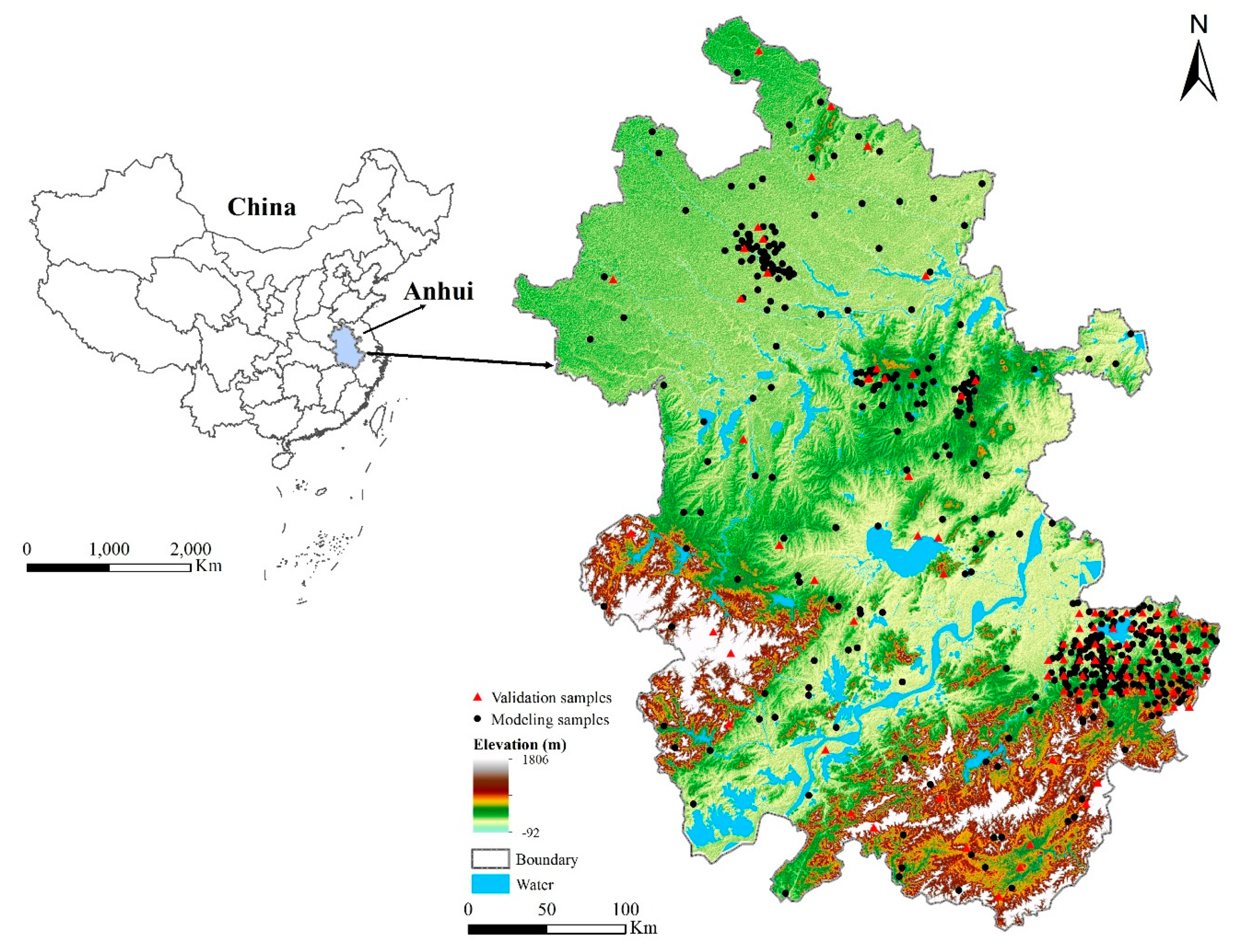
In this paper, the proposed method was applied in predictive mapping of soil organic matter (SOM) content in the topsoil layer in Anhui Province (29°23′44″N – 34°39′5″N, 114°52′35″E – 119°39′37 E″), China. This area was chosen as the case study, because it is a typical area with complex topography and climate conditions.
The study area (Figure 1) was about 1.34 × 10⁵ km2. The terrain was relatively undulating, with elevations ranging from −92 m to 1806 m, and slope gradients between 0° and 50°. The southern and southwestern regions of the study area were mountainous with a rough and variable terrain, while the northern region had a relatively gentle terrain and was mostly plains. The climate condition was in the transition zone between warm temperate and subtropical climates, which is warm and humid in summer and cool and dry in winter. The average annual precipitation ranged from 750 to 2000 mm, and the average temperature was between 14 and 16 °C. The soil parent materials in the study area were complicated and varied, which consisted of basalt, granite, perknite, diorite, schist, shale, sandstone, conglomerate, mudstone, limestone, tuff, and so on. Land use mainly included conifer-broadleaf forests, broadleaf forests, evergreen and deciduous forests, shrubs, and cultivated land mainly located in the northern region.
In this case study, 478 soil sample points collected from multiple sources with uneven distribution were used as the modeling points of DSM, while another 109 soil sample points collected from regular sampling (with a grid of about 10 km × 10 km) and random sampling were used as independent evaluation points (Figure 1).
The environmental factors and corresponding environmental covariates were selected based on domain knowledge and existing DSM studies in this area. For SOM, the climatic condition should have a high influence; meanwhile, SOM is also influenced by topography and parent material according to soil expert knowledge [5,25,27]. Therefore, the environmental factors of climate, terrain, parent material, and vegetation were considered in this case study. A total of nine environmental covariates were selected, including one categorical covariate (i.e., parent material type) and eight continuous covariates (i.e., annual averaged precipitation, annual averaged temperature, moisture index, elevation, slope gradient, planform curvature, profile curvature, and Normalized Difference Vegetation Index (NDVI)) (Table 1).
The covariates of the climate factor (i.e., annual average precipitation and annual average temperature) were generated by inverse distance weighting (IDW) with observation values at 35 weather stations (28 weather stations inside the study area and seven weather stations within 10 km distance to the boundary of study area) from the National Meteorological Information Center. The covariates of the terrain factor were obtained based on Shuttle Radar Topography Mission (SRTM) DEM with a resolution of 90 m. Slope gradient, planform and profile curvatures were derived from DEM with SimDTA [32], a terrain analysis software. NDVI was obtained from the Moderate Resolution Imaging Spectroradiometer (MODIS) vegetation index (with a resolution of 250 m) downloaded from the website (https://lpdaac.usgs.gov). The parent material data was from the 1:500 000 geological map of China. Only for parent material did the source data show NoData for some locations (near lakes). All environmental covariates were resampled to have the same spatial resolution (i.e., 90 m) (Figure 2). Moisture index and NDVI were resampled by the bilinear algorithm implemented in ArcGIS. Parent material data were resampled by the mode within a 3 × 3 window, which was conducted in MATLAB. The resulting original dataset had 16302679 cells with valid values on all covariates over the study area.
3.2. Experimental Design
To evaluate the performance of the proposed SoLIM-FilterNA method, different datasets with diverse distribution of NoData of environmental covariates (so-called test scenarios in this paper) were created based on the original dataset. Among the nine environmental covariates, four topographic covariates of terrain factor (i.e., elevation, slope gradient, planform and profile curvatures) were kept for free of NoData value in this experiment. This was due to the fact that DEM for deriving topographic covariates is increasingly available with high completeness (no NoData value) and accessibility. This setting also prevented the potential situation of having cells with NoData for all environmental covariates in the following experiment.
Test scenarios for the experiment were created by randomly selecting independent evaluation points for setting NoData value on one or several of the remaining five environmental covariates (with one categorical and four continuous covariates) at the individual cell level and the block level, respectively. Among the seven cell-level test scenarios (Table 2), one (continuous variable and categorical variable, respectively) and several (i.e., 2, 3, 4, 5, and 1–5, respectively) of the remaining five environmental covariates were randomly selected for setting NoData value for independent evaluation samples. Seven cell-level scenarios (i.e., T(V1C), T(V1T), T(V2), T(V3), T(V4), T(V5), and T(Vr); see Table 2) were created by setting NoData value for all 109 independent evaluation points, and they were used to compare the performance between the proposed SoLIM-FilterNA method and those methods that can predict the soil value for cells with NoData value for some of environmental covariates (see Section 3.3 below). Besides, one cell-level scenario (i.e., T(Vr-74cell)) was created by setting NoData value for randomly selected variables (1–5) among the five environmental covariates on 74 evaluation points randomly selected from all independent evaluation points (about 70% of the count). T(Vr-74cell) was used to compare the performance between the SoLIM-FilterNA and the method adopting the location-skipping scheme, which cannot predict soil property value on cells with NoData value of environmental covariate.
When cell-level test scenarios simulated the scattered distribution of NoData value in environmental covariates, block-level test scenarios simulated the distribution of blocks with NoData. Four block-level test scenarios (i.e., T(Vr-buffer5), T(Vr-buffer10), T(Vr-buffer15), and T(Vr-buffer25); Table 2) were created by extending the cell-level test scenario T(Vr) to set a buffer (i.e., 5, 10, 15, and 25 cells, respectively) for each of the 109 evaluation points in setting NoData value for the corresponding environmental covariates with NoData value. These block-level test scenarios were used to compare the performance between SoLIM-FilterNA and the methods that can predict soil value of cells with NoData value for part of the environmental covariates.
Note that in the test scenarios, all modeling points were kept without setting NoData value for environmental covariates. This is because normally the real DSM applications only design and adopt those modeling points without NoData value for environmental covariates. The proposed method can handle the modeling points with NoData value for environmental covariates in a similar way to processing the unvisited locations with NoData value for environmental covariates. We believe that current experimental design can appropriately evaluate the performance of the proposed method.
3.3. Evaluation Method
The performance of SoLIM-FilterNA was compared with those from the original SoLIM which takes the location-skipping scheme to simply skip prediction (by marking NoData) of cells with NoData value on any covariate, the SoLIM combining with the void-filling scheme which conducts prediction after (so-called the SoLIM-FillNA method for short), and random forest (RF), respectively.
The SoLIM-FillNA method conducted predictive SOM mapping after NoData value of each individual covariate in the used dataset were filled by interpolation based on a 3 × 3 neighboring window. For continuous covariates, the interpolation was conducted by replacing the NoData value with the average value of valid values in the 3 × 3 window in an iterative manner. For categorical covariates, the NoData value was similarly replaced with the mode in a 3 × 3 window.
Random forest [33], a widely used ensemble learning method, has been successfully used for classification, regression, and other tasks [34,35] and is increasingly applied to DSM. The RF algorithm trains a set of decision trees and generates class from the mode of the classes (classification) or mean prediction (regression) of the individual trees. RF can conduct prediction under the situation with missing data in the input layers. In this study, we used RF by calling the random forest package implemented with the R language. To deal with the NoData value issue, the rfImpute algorithm in the random forest package was first executed to initially impute the NoData as the mean value for continuous variables or the mode for categorical variables. Then, in an iterative manner, randomForest was called to obtain the proximity matrix from the processed input dataset without NoData. In turn, the imputed value for NoData is updated to be the weighted average of valid values with the proximities as weights for continuous covariates or the category with the largest average proximity for categorical covariates. After a given number iterations of this process, a dataset without NoData will be available for RF execution. This way of using RF has shown a good performance when there are missing data in application domains, such as epidemiologic [36] and land-cover classification [37]. To the best of our knowledge, the performance of RF in dealing with the NoData issue in DSM covariates has not been evaluated in detail.
The performance of each method under test was evaluated using quantitative statistics of differences between the SOM observations and the SOM prediction value of each independent evaluation point, including the root mean square error (RMSE; Equation (7)) and mean absolute error (MAE; Equation (8)):
in which and are the predicted value and the observed soil property value at location i, respectively. n is the number of evaluation samples. The comparative evaluations among the methods under test had the same modeling points and the same independent evaluation points. Note that the original SoLIM, taking the location-skipping scheme, simply marked NoData on those cells with NoData value for any environmental covariate. This means that the prediction error from the original SoLIM cannot be calculated for those independent evaluation samples with NoData value on any environmental covariate. Above, the quantitative statistics for the original SoLIM were calculated based on independent evaluation samples with valid values on every environmental covariate (i.e., with the cell-level test scenario T(Vr-74cell)).
Also note that the SoLIM-FilterNA method produced the same error (and thus the same value of individual quantitative statistics) on the same one independent evaluation sample, no matter that the scenario had cell-level NoData or block-level NoData. However, for SoLIM-FillNA or RF, the errors produced on the same one independent evaluation sample under the scenario of cell-level NoData and the block-level scenario, respectively, were different. Therefore, the SoLIM-FilterNA was compared with the original SoLIM in terms of error statistics only under the cell-level test scenario T(Vr-74cell). Based on the same evaluation points, SoLIM-FilterNA under the block-level test scenarios will produce the same RMSE and MAE as SoLIM-FilterNA under the cell-level test scenario T(Vr), while the SoLIM-FillNA or RF will not.
The prediction uncertainty produced by the proposed method was also analyzed quantitatively and qualitatively by comparing with those from the original SoLIM and the SoLIM-FillNA based on the evaluation samples. The prediction uncertainty from RF is usually calculated via confidence intervals and U-test statistics [38,39], which is different from the prediction uncertainty of the SoLIM method. In this experiment, we did not compare the prediction uncertainty from RF with the uncertainty from the SoLIM method.
3.4. Results and Discussion
3.4.1. Under the Cell-Level Test Scenarios
According to RMSE and MAE values from each method under the cell-level test scenarios based on independent evaluation samples (Table 3), the SoLIM-FilterNA method obtained the lowest errors in terms of RMSE among those under test, as well as the lowest MAE, except for the MAE of RF under the T(Vr) scenario. According to RMSE and MAE, the prediction errors from SoLIM-FilterNA increased with the count of covariates setting with NoData value at individual point in the cell-level test scenarios (i.e., the sequence of T(V1C)/T(V1T), T(V2), T(V3), T(V4), till T(V5)), while there was no such phenomenon in SoLIM-FillNA and RF. Such performance of SoLIM-FilterNA was reasonable and better than those of the other methods tested because, in general, the prediction errors should tend to be larger when less environmental covariates can provide valid data for prediction. Following this phenomenon, the RMSE and MAE from SoLIM-FilterNA under the scenario T(Vr) were reasonably between those from SoLIM-FilterNA under the scenario T(V2) and T(V3), while there was no such phenomenon in SoLIM-FillNA and RF. The SoLIM-FillNA method produced the largest RMSE and MAE under each cell-level test scenario because the error in the environmental covariate values was filled by the interpolation algorithm.
Under the cell-level T(Vr-74cell) scenario, SoLIM-FilterNA produced lower RMSE and MAE than that of the original SoLIM (Table 3). Meanwhile, SoLIM-FilterNA could predict soil property values on cells with NoData value for some of environmental covariates, where the original SoLIM produced NoData value in soil prediction. This suggests that SoLIM-FilterNA can guarantee both the completeness of spatial coverage and accuracy of the DSM result.
3.4.2. Under the Block-Level Test Scenarios
Under the block-level test scenarios, the SoLIM-FilterNA method produced the lowest RMSE and MAE compared with SoLIM-FillNA and RF (Table 4). RMSE and MAE from SoLIM-FillNA and RF increased with the buffer size adopted for setting NoData around each of the evaluation points. RMSE and MAE from SoLIM-FillNA were lower than those from RF under block-level test scenarios with smaller buffers (i.e., 5 and 10 cells), but they were larger than those from RF under block-level test scenarios with larger buffers (i.e., 15 and 25 cells) (Table 4). This phenomenon might be because the errors in the environmental covariate values in the center of a block of NoData filled by the interpolation algorithm should be smaller when the block is small. This suggests that SoLIM-FilterNA performed better than SoLIM-FillNA and RF when NoData value in environmental covariates were distributed as spatially continuous blocks.
3.4.3. Prediction Uncertainty
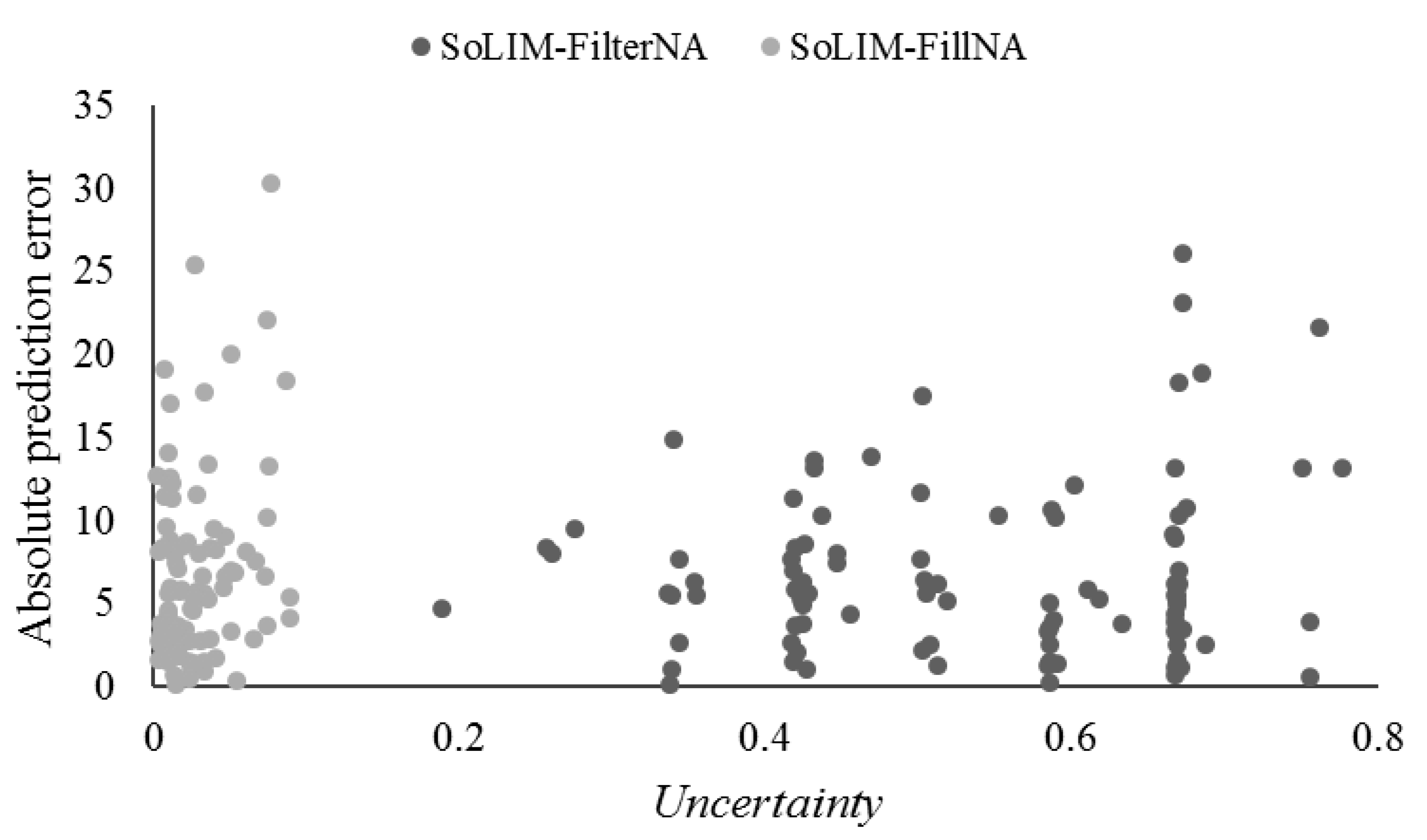
The uncertainty introduced by applying the FilterNA scheme (i.e., Uncertainty_NA as shown in Equation (5)) to SoLIM-FilterNA under the cell-level test scenario T(Vr) was analyzed by plotting against the absolute prediction errors of evaluation samples (Figure 3). In general, the absolute prediction errors increased with the Uncertainty_NA. This means that the uncertainty introduced by applying the FilterNA scheme can be reasonably quantified by SoLIM-FilterNA.
The prediction uncertainty (i.e., Uncertaintyi in Equation (6), which combines the uncertainty introduced by applying the FilterNA scheme and the uncertainty of prediction based on the environmental condition similarities after processing by the FilterNA scheme) produced by SoLIM-FilterNA and SoLIM-FillNA was compared based on 109 independent evaluation samples under the cell-level test scenario T(Vr) (Figure 4).
Generally, the prediction uncertainty from SoLIM-FilterNA could thoroughly depict that the absolute prediction error from SoLIM-FilterNA increased with the prediction uncertainty. Meanwhile, the prediction uncertainty from SoLIM-FillNA could not show similar and reasonable behavior because the uncertainty quantified in SoLIM-FillNA ignored the uncertainty introduced by interpolation for filling NoData value of environmental covariates. This suggests that the prediction uncertainty can be reasonably quantified by SoLIM-FilterNA.
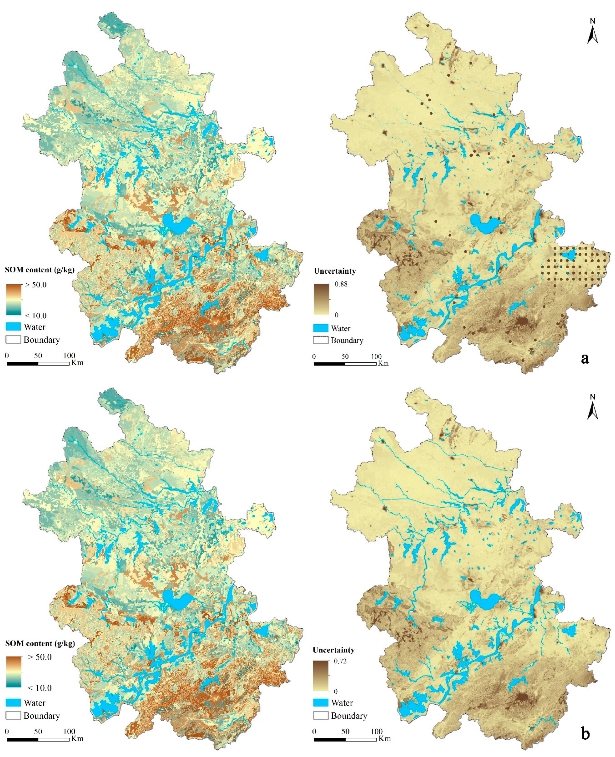
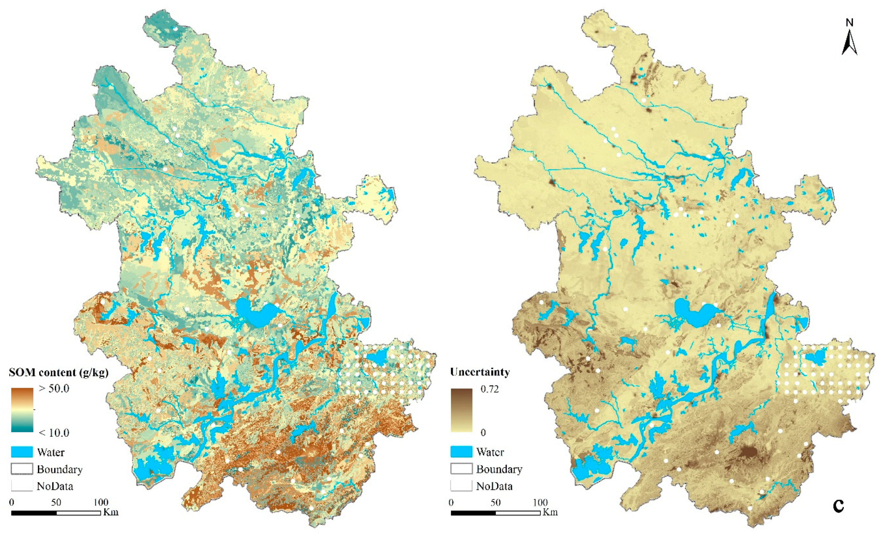
Figure 5 shows the map of SOM prediction and the prediction uncertainty map produced by SoLIM-FilterNA, SoLIM-FillNA, and the original SoLIM under the block-level test scenario T(Vr-buffer25).
By visual comparison of the blocks with NoData in the scenario, the prediction uncertainty values from SoLIM-FilterNA at locations with covariate NoData in the block-level scenario were notably larger than those produced by SoLIM-FillNA with environmental covariates without NoData value. The prediction uncertainty from SoLIM-FilterNA can provide more indicative information on the reliability of prediction (potentially the prediction accuracy) from SoLIM-FilterNA than SoLIM-FillNA, when the original SoLIM cannot predict at these locations.
4. Conclusions and Future Work
The SoLIM-FilterNA method designed based on the FilterNA scheme proposed in this paper can predict soil property values for each cell with NoData value for one or some environmental covariates by using the valid values of other covariates on this cell. The proposed method can guarantee that the spatial coverage of DSM results is as complete as possible. Meanwhile, the proposed method is free from assumptions of distribution or source of NoData value and has neither error nor extra calculation time introduced by interpolation of the NoData value. Thus, the limitations in the existing schemes for dealing with the NoData value of environmental covariates for DSM can be overcome. Furthermore, the prediction uncertainty produced by the proposed SoLIM-FilterNA method considers the uncertainty introduced by ignoring environmental covariates with NoData value at each individual location. Such uncertainty results can indicate the reliability of soil prediction by the proposed method. As shown in the experimental results, the proposed FilterNA scheme, as well as the proposed SoLIM-FilterNA method, can deal with the issue of NoData value of environmental covariates in DSM over a large area. Future work will focus on how to combine the proposed FilterNA scheme with other widely used DSM methods over large area.
Author Contributions
All authors gave substantial contributions to this work. Conceptualization was conducted by Nai-Qing Fan, A-Xing Zhu, and Cheng-Zhi Qin. Formal analysis, investigation, methodology, validation and result analysis were conducted by Nai-Qing Fan, Cheng-Zhi Qin, and Peng Liang. Writing—original draft preparation was conducted by Nai-Qing Fan. Writing—review and editing were conducted by all authors. Supervision, project administration and funding acquisition were conducted by A-Xing Zhu and Cheng-Zhi Qin. All authors have read and agreed to the published version of the manuscript.
Funding
This research was funded by the National Natural Science Foundation of China (No. 41431177, 41871300) and Chinese Academy of Sciences (Project No. XDA23100503).
Acknowledgments
We thank supports from the Priority Academic Program Development of Jiangsu Higher Education Institutions (PAPD), and the Outstanding Innovation Team in Colleges and Universities in Jiangsu Province, China. Supports to A-Xing Zhu through the Vilas Associate Award, the Hammel Faculty Fellow Award, and the Manasse Chair Professorship from the University of Wisconsin-Madison are greatly appreciated.
Conflicts of Interest
The authors declare no conflict of interest.
References
- Goodchild, M.F.; Parks, B.O.; Steyaert, L.T. Environmental Modeling with GIS; Oxford University Press: New York, NY, USA, 1993. [Google Scholar]
- Shani, U.; Ben-Gal, A.; Tripler, E.; Dudley, L.M. Plant response to the soil environment: An analytical model integrating yield, water, soil type, and salinity. Water Resour. Res. 2007, 43, W08418. [Google Scholar] [CrossRef]
- Grunwald, S.; Thompson, J.; Boettinger, J. Digital soil mapping and modeling at continental scales: Finding solutions for global issues. Soil Sci. Soc. Am. J. 2011, 75, 1201–1213. [Google Scholar] [CrossRef]
- Stoorvogel, J.J.; Bakkenes, M.; Temme, A.J.; Batjes, N.H.; ten Brink, B.J. S-world: A global soil map for environmental modelling. Land Degrad. Dev. 2017, 28, 22–33. [Google Scholar] [CrossRef]
- McBratney, A.B.; Santos, M.L.M.; Minasny, B. On digital soil mapping. Geoderma 2003, 117, 3–52. [Google Scholar] [CrossRef]
- Zhu, A.X.; Hudson, B.; Burt, J.; Lubich, K.; Simonson, D. Soil mapping using GIS, expert knowledge, and fuzzy logic. Soil Sci Soc. Am. J. 2001, 65, 1463–1472. [Google Scholar] [CrossRef] [Green Version]
- Minasny, B.; McBratney, A.B. Digital soil mapping: A brief history and some lessons. Geoderma 2016, 264, 301–311. [Google Scholar] [CrossRef]
- Zhu, A.X.; Band, L.; Vertessy, R.; Dutton, B. Derivation of soil properties using a soil land inference model (SoLIM). Soil Sci Soc. Am. J. 1997, 61, 523–533. [Google Scholar] [CrossRef]
- Ishioka, T. Imputation of missing values for semi-supervised data using the proximity in random forests. In Proceedings of the 14th International Conference on Information Integration and Web-based Applications & Services, Bali, Indonesia, 3–5 December 2012; pp. 319–322. [Google Scholar]
- Taghizadeh-Mehrjardi, R.; Minasny, B.; Sarmadian, F.; Malone, B. Digital mapping of soil salinity in Ardakan region, central Iran. Geoderma 2014, 213, 15–28. [Google Scholar] [CrossRef]
- Little, R.J.; Rubin, D.B. Statistical Analysis with Missing Data, 2nd ed.; John Wiley & Sons: Hoboken, NJ, USA, 2019. [Google Scholar]
- Hugelius, G.; Tarnocai, C.; Broll, G.; Canadell, J.; Kuhry, P.; Swanson, D. The Northern Circumpolar Soil Carbon Database: Spatially distributed datasets of soil coverage and soil carbon storage in the northern permafrost regions. Earth Syst. Sci. Data 2013, 5, 3–13. [Google Scholar] [CrossRef] [Green Version]
- Hengl, T.; Gruber, S.; Shrestha, D.P. Reduction of errors in digital terrain parameters used in soil-landscape modelling. Int. J. Appl. Earth Obs. Geoinf. 2004, 5, 97–112. [Google Scholar] [CrossRef]
- Grimm, R.; Behrens, T.; Marker, M.; Elsenbeer, H. Soil organic carbon concentrations and stocks on Barro Colorado Island - Digital soil mapping using Random Forests analysis. Geoderma 2008, 146, 102–113. [Google Scholar] [CrossRef]
- Hengl, T.; Heuvelink, G.B.; Kempen, B.; Leenaars, J.G.; Walsh, M.G.; Shepherd, K.D.; Sila, A.; MacMillan, R.A.; Mendes de Jesus, J.; Tamene, L.; et al. Mapping Soil Properties of Africa at 250 m Resolution: Random Forests Significantly Improve Current Predictions. PLoS ONE 2015, 10, e0125814. [Google Scholar] [CrossRef] [PubMed]
- Vågen, T.G.; Winowiecki, L.A.; Tondoh, J.E.; Desta, L.T.; Gumbricht, T. Mapping of soil properties and land degradation risk in Africa using MODIS reflectance. Geoderma 2016, 263, 216–225. [Google Scholar] [CrossRef] [Green Version]
- McBratney, A.B.; Walvoort, D.J.J. Generalised Linear Model Kriging: A generic framework for kriging with secondary data. In Proceedings of the Pedometrics 2001 4th Conference of the Working Group on Pedometric of the IUSS, Ghent, Belgium, 19–21 September 2001. [Google Scholar]
- Hengl, T.; de Jesus, J.M.; MacMillan, R.A.; Batjes, N.H.; Heuvelink, G.B.; Ribeiro, E.; Samuel-Rosa, A.; Kempen, B.; Leenaars, J.G.; Walsh, M.G.; et al. SoilGrids1km—global soil information based on automated mapping. PLoS ONE 2014, 9, e105992. [Google Scholar] [CrossRef] [PubMed] [Green Version]
- Vaysse, K.; Lagacherie, P. Evaluating digital soil mapping approaches for mapping GlobalSoilMap soil properties from legacy data in Languedoc-Roussillon (France). Geoderma Reg. 2015, 4, 20–30. [Google Scholar] [CrossRef]
- Hengl, T.; Mendes de Jesus, J.; Heuvelink, G.B.; Ruiperez Gonzalez, M.; Kilibarda, M.; Blagotic, A.; Shangguan, W.; Wright, M.N.; Geng, X.; Bauer-Marschallinger, B.; et al. SoilGrids 250 m: Global gridded soil information based on machine learning. PLoS ONE 2017, 12, e0169748. [Google Scholar] [CrossRef] [Green Version]
- Ließ, M. Sampling for regression-based digital soil mapping: Closing the gap between statistical desires and operational applicability. Spat. Stat. 2015, 13, 106–122. [Google Scholar] [CrossRef]
- Zhu, A.X.; Liu, J.; Du, F.; Zhang, S.J.; Qin, C.Z.; Burt, J.; Behrens, T.; Scholten, T. Predictive soil mapping with limited sample data. Eur. J. Soil Sci. 2015, 66, 535–547. [Google Scholar] [CrossRef]
- Qin, C.Z.; Zhu, A.X.; Qiu, W.L.; Lu, Y.J.; Li, B.L.; Pei, T. Mapping soil organic matter in small low-relief catchments using fuzzy slope position information. Geoderma 2012, 171–172, 64–74. [Google Scholar] [CrossRef]
- Zhu, A.X.; Qi, F.; Moore, A.; Burt, J.E. Prediction of soil properties using fuzzy membership values. Geoderma 2010, 158, 199–206. [Google Scholar] [CrossRef]
- Zhu, A.X.; Lü, G.N.; Liu, J.; Qin, C.Z.; Zhou, C.H. Spatial prediction based on Third Law of Geography. Ann. GIS 2018, 24, 225–240. [Google Scholar] [CrossRef]
- Yang, L.; Zhu, A.X.; Zhao, Y.G.; Li, D.C.; Zhang, G.L.; Zhang, S.J.; Band, L.E. Regional Soil Mapping Using Multi-Grade Representative Sampling and a Fuzzy Membership-Based Mapping Approach. Pedosphere 2017, 27, 344–357. [Google Scholar] [CrossRef]
- An, Y.M.; Yang, L.; Zhu, A.X.; Qin, C.Z.; Shi, J.J. Identification of representative samples from existing samples for digital soil mapping. Geoderma 2018, 311, 109–119. [Google Scholar] [CrossRef]
- Zhu, A.X.; Band, L.E. A knowledge-based approach to data integration for soil mapping. Can. J. Remote Sens. 1994, 20, 408–418. [Google Scholar] [CrossRef]
- Zhu, A.X. A personal construct-based knowledge acquisition process for natural resource mapping. Int. J. Geogr. Inf. Sci. 1999, 13, 119–141. [Google Scholar] [CrossRef]
- Minasny, B.; McBratney, A.B.; Malone, B.P.; Wheeler, I. Digital Mapping of Soil Carbon. Adv. Agron. 2013, 118, 1–47. [Google Scholar]
- Zhu, A.X. Measuring uncertainty in class assignment for natural resource maps under fuzzy logic. Photogramm. Eng. Remote Sens. 1997, 63, 1195–1202. [Google Scholar]
- Qin, C.Z.; Lu, Y.J.; Bao, L.L.; Zhu, A.X.; Qiu, W.L.; Cheng, W.M. Simple digital terrain analysis software (SimDTA 1.0) and its application in fuzzy classification of slope positions. J. Geo-Inf. Sci. 2009, 11, 737–743, (in Chinese with English abstract). [Google Scholar] [CrossRef]
- Breiman, L. Random forests. Mach. Learn. 2001, 45, 5–32. [Google Scholar] [CrossRef] [Green Version]
- Liaw, A.; Wiener, M. Classification and regression by randomForest. R News 2002, 2, 18–22. [Google Scholar]
- Genuer, R.; Poggi, J.-M.; Tuleau-Malot, C. Variable selection using random forests. Pattern Recognit. Lett. 2010, 31, 2225–2236. [Google Scholar] [CrossRef] [Green Version]
- Pantanowitz, A.; Marwala, T. Evaluating the Impact of Missing Data Imputation through the use of the Random Forest Algorithm. arXiv 2008, arXiv:0812.2412. [Google Scholar]
- Rodriguez-Galiano, V.F.; Ghimire, B.; Rogan, J.; Chica-Olmo, M.; Rigol-Sanchez, J.P. An assessment of the effectiveness of a random forest classifier for land-cover classification. J. Photogramm. Remote Sens. 2012, 67, 93–104. [Google Scholar] [CrossRef]
- Mentch, L.; Hooker, G. Quantifying Uncertainty in Random Forests via Confidence Intervals and Hypothesis Tests. J. Mach. Learn. Res. 2016, 17, 1–41. [Google Scholar]
- Vaysse, K.; Lagacherie, P. Using quantile regression forest to estimate uncertainty of digital soil mapping products. Geoderma 2017, 291, 55–64. [Google Scholar] [CrossRef]
Figure 1.
Map of the study area (Anhui Province) and soil samples.

Figure 2.
Maps of environmental covariates in the study area: (a) annual averaged precipitation; (b) annual averaged temperature; (c) moisture index; (d) elevation; (e) planform curvature; (f) profile curvature; (g) slope gradient; (h) NDVI; (i) parent material (legend of parent material: 1. acid plutonic, volcanic or metamorphic rocks, 2. pyroclastic rocks, 3. Sandstone, 4. psammite or arenite, 5. calcareous rocks, 6. fine-silt and sandy clay, 7. intermediate volcanic and plutonic rocks, 8. silt clay and clayey silt interbed, 9. basic metamorphic, volcanic or plutonic rocks, 10. fine-silt and clayey silt, 11. fine-silt and sandy gravel soils, 13. sandy clay, 14. wormlike boulder clay or gravelly clay, the gravel has abrasion faces and striations, 15. psephite or rudite, 16. top with silt clay and bottom with gravelly medium-fine sandy, silt clay).
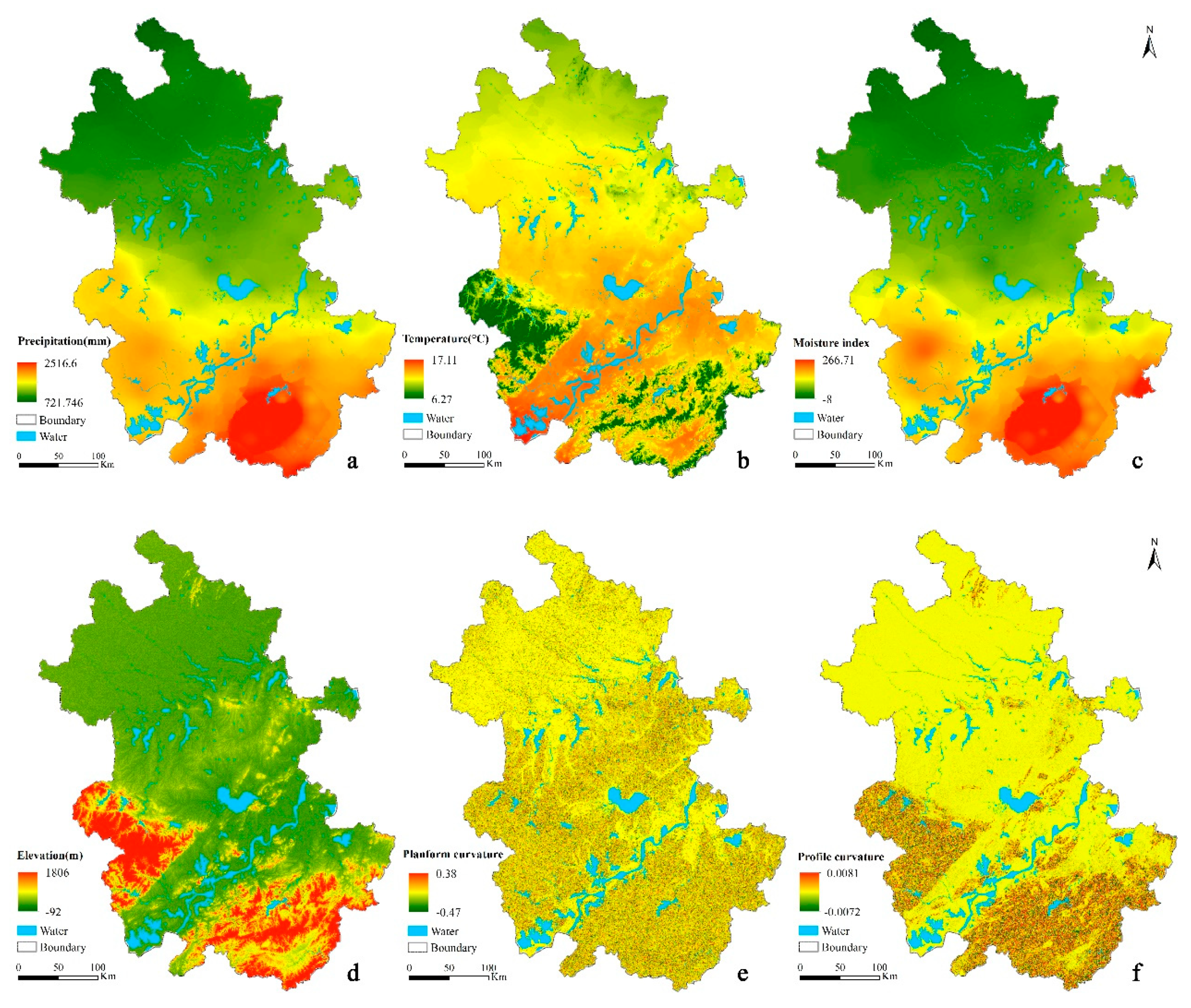
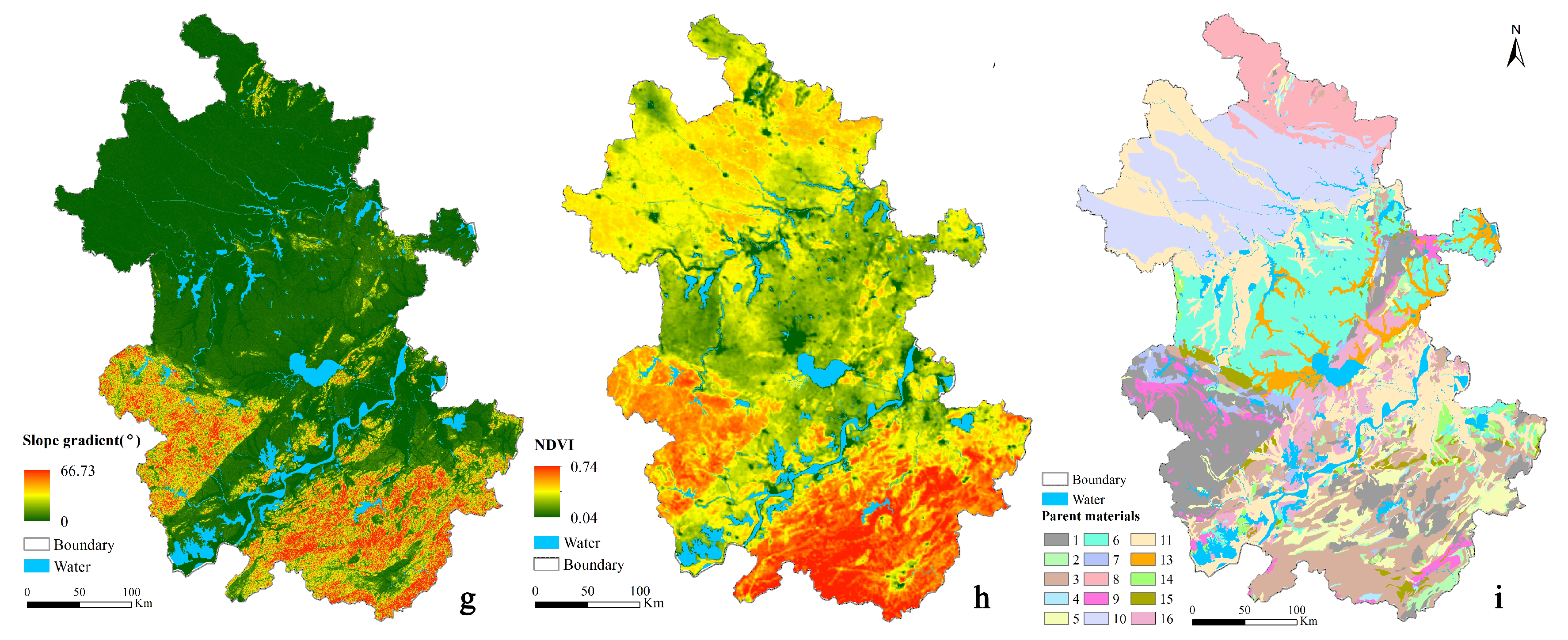
Figure 3.
Uncertainty_NA against the absolute prediction errors of evaluation samples by SoLIM-FilterNA under the cell-level test scenario T(Vr).
Figure 3.
Uncertainty_NA against the absolute prediction errors of evaluation samples by SoLIM-FilterNA under the cell-level test scenario T(Vr).
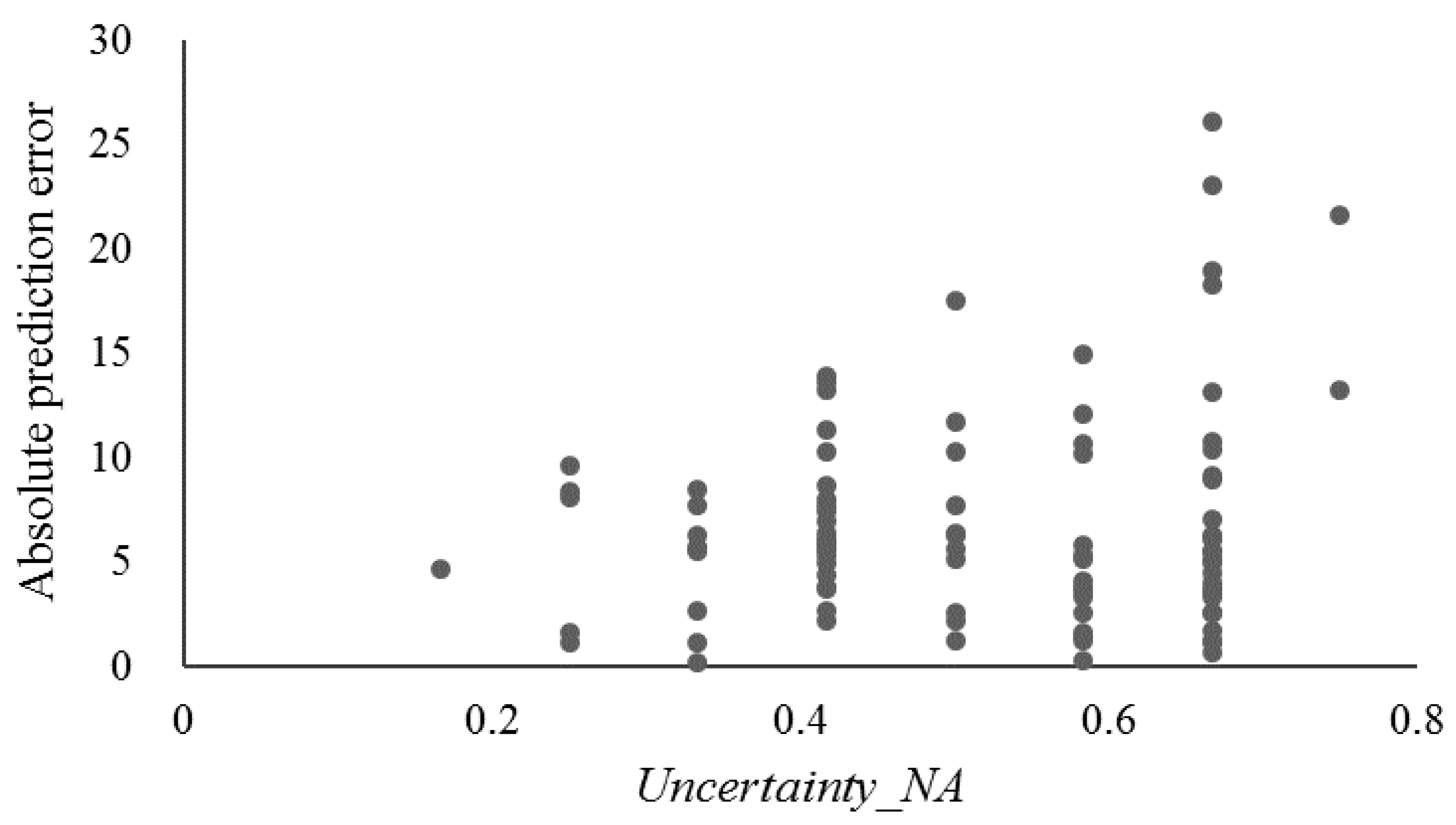
Figure 4.
Distribution of prediction uncertainty of evaluation samples derived from SoLIM-FilterNA and the original SoLIM under the cell-level test scenario T(Vr).
Figure 4.
Distribution of prediction uncertainty of evaluation samples derived from SoLIM-FilterNA and the original SoLIM under the cell-level test scenario T(Vr).

Figure 5.
Maps of the top-layer SOM (g/kg) prediction and the corresponding uncertainty under the block-level test scenario T(Vr-buffer25) by (a) SoLIM-FilterNA, (b) SoLIM-FillNA, and (c) the original SoLIM.
Figure 5.
Maps of the top-layer SOM (g/kg) prediction and the corresponding uncertainty under the block-level test scenario T(Vr-buffer25) by (a) SoLIM-FilterNA, (b) SoLIM-FillNA, and (c) the original SoLIM.


Table 1.
Environmental covariates used in the case study.
| Environmental Factor | Environmental Covariates | Data Type | Data Source | Original Resolution | Algorithm |
|---|---|---|---|---|---|
| Climate | Annual averaged precipitation | Continuous | Observations from National Meteorological station | Station | IDW |
| Annual averaged temperature | |||||
| Moisture index | Continuous | http://www.resdc.cn | 500 m | Resample | |
| Terrain | Elevation | Continuous | SRTM DEM | 90 m | -- |
| Slope gradient | Continuous | SRTM DEM | 90 m | SimDTA [32] | |
| Planform curvature | |||||
| Profile curvature | |||||
| Vegetation | NDVI | Continuous | MODIS | 250 m | Resample |
| Parent material | Parent material | Categorical | http://www.ngac.org.cn | 1:500,000 | Resample |
Table 2.
Test scenarios with NoData value randomly set for one or several of the five environmental covariates at the cell level and the block level, respectively.
Table 2.
Test scenarios with NoData value randomly set for one or several of the five environmental covariates at the cell level and the block level, respectively.
| Test Scenario | Level | Covariate Setting NoData | Count of Cells with NoData Set on at Least One Covariate | |
|---|---|---|---|---|
| Count | Date Type | |||
| T(V1C) | Cell-level | 1 | Continuous | 109 (i.e., all independent evaluation points) |
| T(V1T) | Cell-level | 1 | Categorical (Type) | 109 |
| T(V2) | Cell-level | 2 | Random | 109 |
| T(V3) | Cell-level | 3 | Random | 109 |
| T(V4) | Cell-level | 4 | Random | 109 |
| T(V5) | Cell-level | 5 | Random | 109 |
| T(Vr) | Cell-level | 1~5 | Random | 109 |
| T(Vr-74cell) | Cell-level | 1~5 | Random | 74 (evaluation points randomly selected) |
| T(Vr-buffer5) | Block-level | same as T(Vr) | 109 evaluation points with their buffer of 5 cells | |
| T(Vr-buffer10) | Block-level | same as T(Vr) | 109 evaluation points with their buffer of 10 cells | |
| T(Vr-buffer15) | Block-level | same as T(Vr) | 109 evaluation points with their buffer of 15 cells | |
| T(Vr-buffer25) | Block-level | same as T(Vr) | 109 evaluation points with their buffer of 25 cells | |
Note: Regarding the name of the test scenario T(V1C), “T(.)” means test scenario, “V1C” means that one continuous variable ("V1T” for one categorical variable, and “Vr” for randomly selected 1~5 variables) among the five environmental covariates was selected for setting NoData value. Other test scenarios are named in a similar way.
Table 3.
RMSE and MAE of the errors on the top-layer SOM (g/kg) predicted by different methods under cell-level test scenarios.
Table 3.
RMSE and MAE of the errors on the top-layer SOM (g/kg) predicted by different methods under cell-level test scenarios.
| Methods | Error Statistics | Test Scenario | |||||||
|---|---|---|---|---|---|---|---|---|---|
| T(V1C) | T(V1T) | T(V2) | T(V3) | T(V4) | T(V5) | T(Vr) | T(Vr-74cell) | ||
| SoLIM-FilterNA | RMSE | 8.334 | 8.253 | 8.447 | 8.654 | 8.666 | 8.681 | 8.556 | 9.052 |
| MAE | 6.786 | 6.580 | 6.727 | 6.850 | 6.916 | 6.982 | 6.877 | 7.179 | |
| SoLIM-FillNA | RMSE | 8.861 | 8.866 | 9.056 | 9.054 | 9.056 | 9.071 | 9.058 | – |
| MAE | 6.915 | 6.921 | 7.061 | 7.057 | 7.059 | 7.102 | 7.064 | – | |
| RF | RMSE | 8.414 | 8.602 | 8.682 | 8.703 | 8.710 | 8.727 | 8.660 | – |
| MAE | 6.641 | 6.897 | 7.057 | 7.027 | 6.975 | 6.733 | 7.038 | – | |
| original SoLIM | RMSE | – | – | – | – | – | – | – | 9.564 |
| MAE | – | – | – | – | – | – | – | 7.816 | |
Table 4.
Error statistics of the top-layer SOM (g/kg) predicted by different methods under block-level test scenarios, evaluated based on 109 independent evaluation samples.
Table 4.
Error statistics of the top-layer SOM (g/kg) predicted by different methods under block-level test scenarios, evaluated based on 109 independent evaluation samples.
| Methods | Error Statistics | Block-Level Test Scenario | |||
|---|---|---|---|---|---|
| T(Vr-Buffer5) | T(Vr-Buffer10) | T(Vr-Buffer15) | T(Vr-Buffer25) | ||
| SoLIM-FilterNA | RMSE | 8.556 | 8.556 | 8.556 | 8.556 |
| MAE | 6.877 | 6.877 | 6.877 | 6.877 | |
| SoLIM-FillNA | RMSE | 9.145 | 9.183 | 9.512 | 10.199 |
| MAE | 7.133 | 7.210 | 7.329 | 7.278 | |
| RF | RMSE | 9.262 | 9.325 | 9.470 | 9.655 |
| MAE | 7.532 | 7.619 | 7.793 | 8.254 | |
© 2020 by the authors. Licensee MDPI, Basel, Switzerland. This article is an open access article distributed under the terms and conditions of the Creative Commons Attribution (CC BY) license (http://creativecommons.org/licenses/by/4.0/).
Share and Cite
MDPI and ACS Style
Fan, N.-Q.; Zhu, A.-X.; Qin, C.-Z.; Liang, P. Digital Soil Mapping over Large Areas with Invalid Environmental Covariate Data. ISPRS Int. J. Geo-Inf. 2020, 9, 102. https://0-doi-org.brum.beds.ac.uk/10.3390/ijgi9020102
AMA Style
Fan N-Q, Zhu A-X, Qin C-Z, Liang P. Digital Soil Mapping over Large Areas with Invalid Environmental Covariate Data. ISPRS International Journal of Geo-Information. 2020; 9(2):102. https://0-doi-org.brum.beds.ac.uk/10.3390/ijgi9020102
Chicago/Turabian StyleFan, Nai-Qing, A-Xing Zhu, Cheng-Zhi Qin, and Peng Liang. 2020. "Digital Soil Mapping over Large Areas with Invalid Environmental Covariate Data" ISPRS International Journal of Geo-Information 9, no. 2: 102. https://0-doi-org.brum.beds.ac.uk/10.3390/ijgi9020102
Note that from the first issue of 2016, this journal uses article numbers instead of page numbers. See further details here.