Article

Slope Hazard Monitoring Using High-Resolution Satellite Remote Sensing: Lessons Learned from a Case Study

1
Lyles School of Civil Engineering, Purdue University, West Lafayette, IL 47907, USA
2
Virginia Department of Transportation, 530 Edgemont Road, Charlottesville, VA 22903, USA
*
Author to whom correspondence should be addressed.
ISPRS Int. J. Geo-Inf. 2020, 9(2), 131; https://0-doi-org.brum.beds.ac.uk/10.3390/ijgi9020131
Submission received: 3 December 2019 / Revised: 22 January 2020 / Accepted: 27 January 2020 / Published: 23 February 2020
(This article belongs to the Special Issue Geospatial Approaches to Landslide Mapping and Monitoring)

Abstract

:
In this study, a highway slope monitoring project for a section of US highway I-77 in Virginia was carried out with the InSAR technique. This paper attempts to provide insights into the complete and practical solution for the monitoring project, including two parts: what to consider for selecting the optimal satellites and configurations for the given area of interest (AoI) and budget; and how to best process the selected data for the monitoring purposes. To answer the first question, the simulated geometric distortion map, cumulative change detection map, intensity map, interferograms and coherence maps from all available historical datasets were generated. The satellite configuration that gives the best coherence and least geometric distortion with the given budget was selected for the monitoring project. For this project, it was the X-band COSMO stripmap with 3 m resolution and eight-days revisit time. To answer the second question, a multi-temporal InSAR (MTInSAR) was applied to retrieve the settlement time series of the slopes along the highway. Several special techniques were applied to increase the level of confidence, i.e., dividing AoI into smaller and independent areas, using a non-linear approach, etc. Finally, fieldwork was carried out for the interpretation and validation of the results. The AoI was overall stable, though some local changes were detected by the SAR signal which were validated by the fieldwork.

1. Introduction

One of the major safety concerns to traveling public is the slope stability along the roads. Particularly, in mountainous areas with steep slopes, landslides pose potential threats to public safety. Early detection of impending ground displacement may provide valuable insights to slope hazards assessment and result in improved safety along a transportation corridor.
The conventional way of detecting slope movement is performed with point-wise sensors (e.g., slope inclinometer or GPS receivers) at pre-identified locations that are considered geologically vulnerable. These measurements are accurate, but hardly sufficient over the entire area of interest (AoI).
A popular alternative is to use interferometric synthetic aperture radar (InSAR) and multi-temporal InSAR (MTInSAR) [1]. The technology stands out for its all-time, wide-area, high-accuracy monitoring capabilities as well as the good cost-benefit ratio. As early as 2006, the U.S. Department of Transportation (DOT) has reported using InSAR for monitoring slopes along the interstate highways [2]. In the recent decade, there have been advancements at both the hardware level and the algorithm level [1]. With the availability of high-resolution SAR satellites such as TerraSAR-X (TSX) and COSMO-SkyMed (COSMO), it is theoretically possible to turn every 2-meter-pixel inside a 1000   km 2 area (the approximate coverage of TSX or CSK stripmap mode) into a GPS measurement with millimeters accuracy [3,4]. This opens up numerous new possibilities in earth monitoring projects.
The number of ground monitoring applications with InSAR grew unprecedentedly in the last decade. Simply by looking at the published papers, InSAR and MTInSAR have contributed to a variety of fields [5]: geology, geophysics, oil and gas, mining, and most importantly, civil engineering. Among the civil engineering applications, the topics covered but not limited to buildings, railroads, pipelines, tunnels, and sinkholes. One factor that contributes to the success of the field is the advancements of SAR satellites and the accumulation of the archived imageries. Ten years ago when there were only less than a handful of SAR satellites in space, a civil engineering project such as monitoring a slope might only reach the phase of proof-of-concept with low-resolution data (both spatial and temporal). Nowadays, with more operational satellites, it is possible to monitor almost anywhere on earth with plenty of options.
Naturally, when more choices are available, an important question arises: what should the best satellite and the best configuration be for a given project? To expand into a few technical questions, we could have:
  • What is the most suitable wavelength, C, X or L band?
  • What is the best incidence angle?
  • What is the proper revisit frequency?
  • Ascending or descending?
  • What resolution can be accepted?
  • What acquisition mode is better, i.e., stripmap or spotlight?
  • What approach should be used for processing, i.e., differential InSAR (DInSAR) [6], MTInSAR [7], small baseline subset (SBaS) [8], or others [5]?
In an ideal case, it is desired to have all the available configurations (in addition, a decomposition can be performed to determine vertical and horizontal movement [9] by having both ascending and descending track). However, for a real-life engineering project that comes with a budget, the question of how to choose the best configuration(s) becomes important.
In the last decade, the U.S. DOTs initiated a number of InSAR monitoring projects, to name a few, see [10,11,12,13,14]. The awareness of using InSAR along with other conventional surveying techniques for the civil engineering and transportation industry has been growing ever since. As early as in 2006, the U.S. DOT provided guidance for the commercial use of InSAR data in highway slope stability monitoring [2]. The valuable part of [2] is its focus on the practical considerations in using InSAR data rather than just accentuating its theoretical advantages. The ideas in [2] also lead to part of this manuscript, with the consideration of the satellites that were launched after 2006. On the other side, most of the aforementioned DOT projects involving InSAR and MTInSAR applications focused on the processing methodologies and post-analysis. Very few focused on the step that came before all that: the efforts in selecting the most suitable satellite and the optimal configuration. For some of the projects, the reason behind the choice was usually straightforward: to use one or all available data (in most cases this meant only the free ones, i.e., Sentinel-1). However, for a live monitoring project where one can choose from all the available commercial satellites with a given budget, the “shopping” becomes especially important.
Therefore, for a big part of this study, the following open question is thoroughly discussed: for the purpose of monitoring the highway slopes, what is the optimal satellite configuration?
As far as InSAR technology is concerned, the following questions are raised:
  • What is the configuration that gives the best resolution for the AoI (both spatial and temporal)?
  • What is the configuration that gives the best sensitivity of the measurement to the satellite line of sight (LoS)?
  • What is the configuration that gives the best signal–noise ratio (SNR) for the AoI?
In this study, these questions are answered with respect to a monitoring project that involved a section of the U.S. interstate highway I-77 and the adjacent slopes. The project was divided into two parts:
  • Evaluate all available satellite sources, then decide the optimal satellite and configuration for this project;
  • Run MTInSAR for the given AoI and interpret the results.
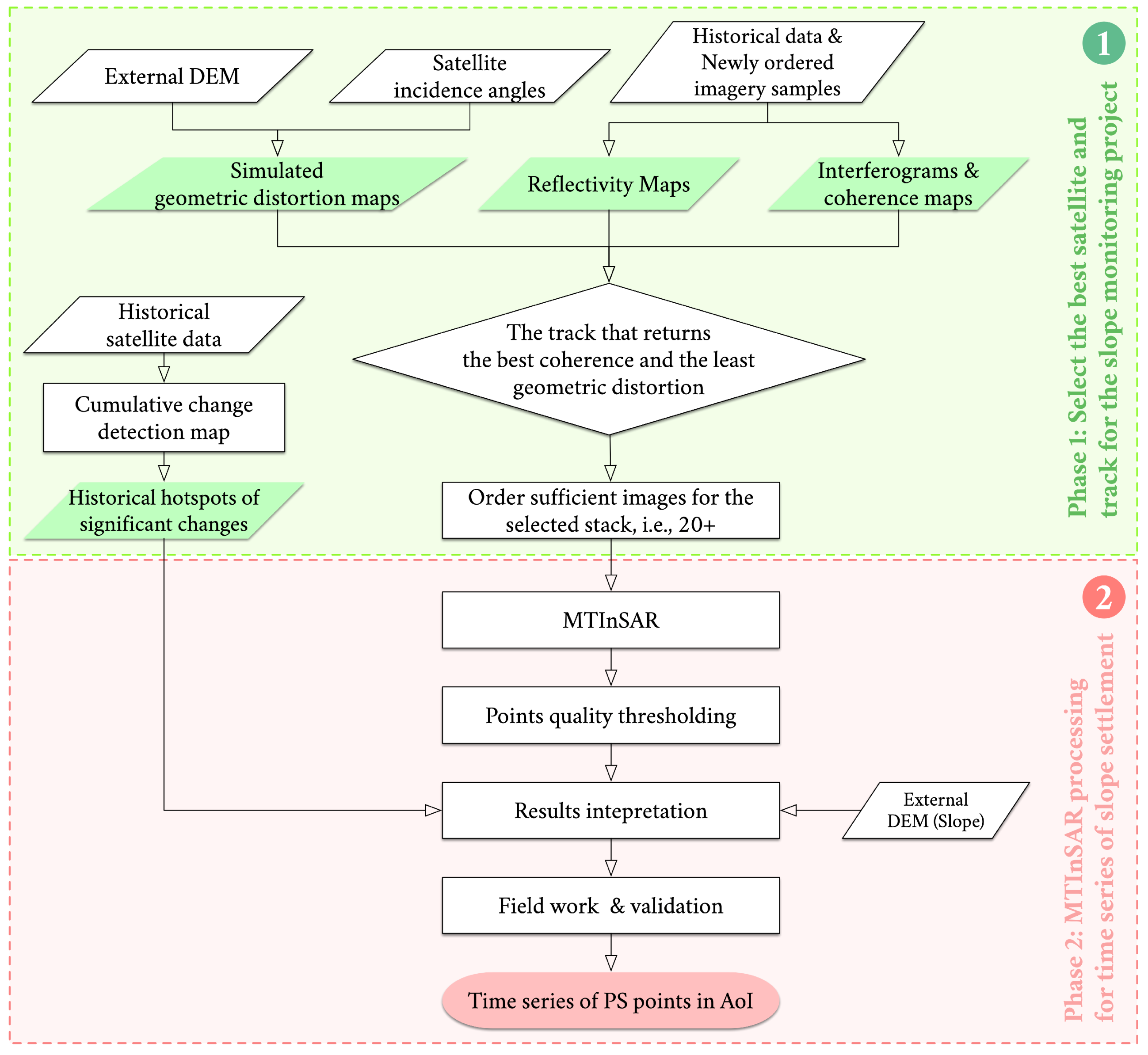
This article is divided into six sections. Section 2 discusses the workflow of the entire project. Section 4 reviews the key methodologies. Section 4 shows the area of interest and available dataset. Section 5 and Section 6 show the result and some interpretation. Section 7 and Section 8 give the discussion and conclusion.

2. Workflow

As shown in Figure 1, there are two phases for this study. Phase 1 is the evaluation of the best satellite configuration based on available options. Phase 2 is MTInSAR processing.

2.1. Phase 1: Evaluate the Most Appropriate Satellite and Configuration

Phase one selects the best configuration for the longer-term monitoring plan in phase 2. The steps are as follows:
  • Generate the simulated geometric distortion map from the external digital elevation model (DEM), satellite resolution and incidence angle;
  • Calculate the cumulative change detection map from historical data, and label a list of historical hotspots that require special attention for MTInSAR processing;
  • (If budget is available) Order a couple of images from the candidate satellite tracks and process the reflectivity maps, interferograms and coherence maps. Cross-check with the simulated geometric distortion map to understand if the results are consistent with the simulated geometric distortion map;
  • Select the satellite and track that: (a) has the suitable spatial resolution for the monitoring target; and (b) has the best coherence in the AoI and at the slopes of interests (SoI).

2.2. Phase 2: Multi-Temporal Analysis with the Selected Satellite Configuration

Phase 2 is the MTInSAR process. The steps are as folllows:
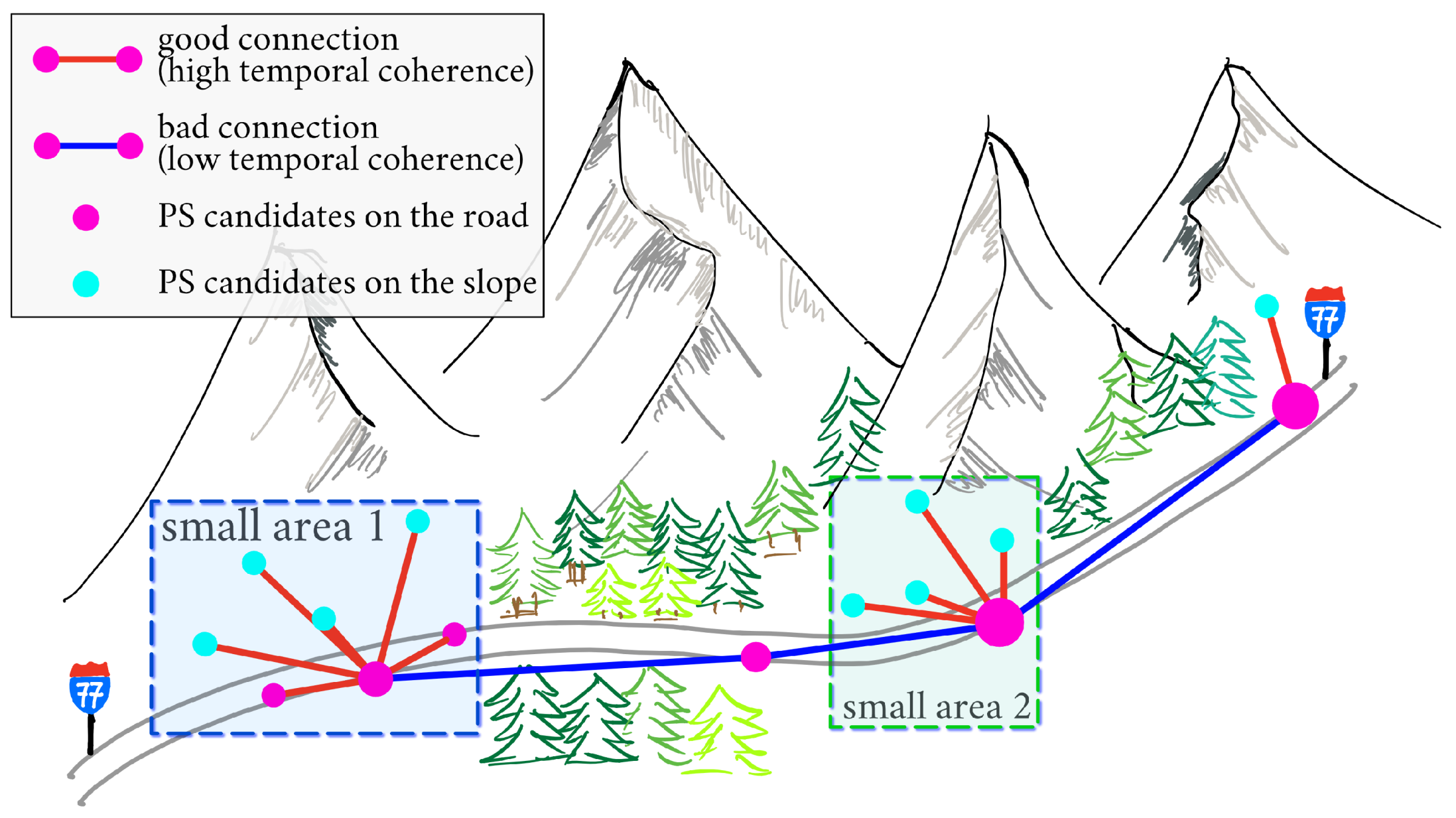
  • Divide the AoI into smaller areas. Each small area is at most 1 to 2 kilometers. Do the MTInSAR processing (Section 3.4);
  • Determine a suitable quality threshold based on the temporal coherence of the points (Section 3.4.3);
  • Inspect the time series of output points. Signs of strong deformation are carefully studied, including also fieldwork as part of the validation;
  • Deliver the result as the deformation map (to the Virginia Department of Transportation in this example).
The reason for dividing the AoI into smaller areas is the following. In the conventional MTInSAR processing [7], the construction and inversion of the network are done on the entire area of interest. One of the keys is the quality of the network connection. For example, if two smaller clusters of points in the whole network are connected badly (in terms of temporal coherence), then the network inversion is likely to go bad and propagate the error (Figure 2). For the inversion to be successful, the vertices should distribute densely and evenly in space to assure the quality of the arc and the redundancy of network inversion. However, in this project, the majority of the AoI is heavily vegetated. By the nature of persistent scatterers (PS), it is only possible to get PS points on the highway surface and at barren rock slopes. In other words, the connection between the slopes would be less than optimal due to the lack of points and the uneven distribution. The inversion of the network is thus more likely to be unsuccessful. The solution would be to perform the following. For each individual slope, a lot of PS candidates can be found with a relatively good connection to the nearby reference point located on the highway. We already knew from the Virginia Department of Transportation (VDOT) that the highway is relatively stable, and the slopes are the potential hazards to watch out for. Therefore, a practical approach would be dividing the entire 8-mile-AoI into smaller areas. For each area the MTInSAR process is done independently, and the point with the lowest amplitude dispersion [7] on the highway is used as the reference point for that small area. Figure 2 illustrates this approach.

3. Methodology

This section covers the important concepts and methods used in this project. Most are already well defined in previous research, so this chapter will focus on how these methods contribute to this particular project.

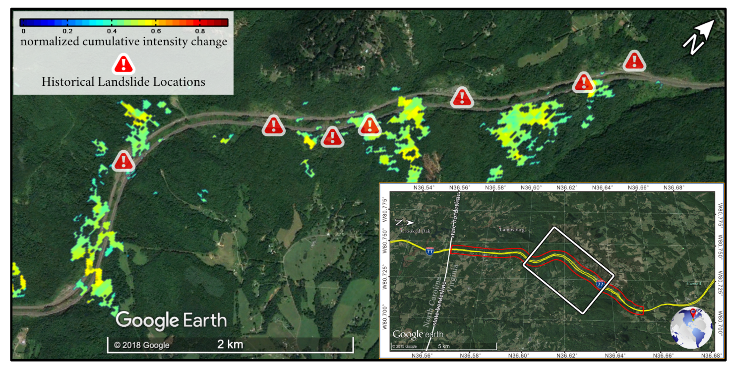
3.1. Cumulative Change Detection Map

The amplitude of SAR imagery depicts the intensity of the received signal from the ground object. The amplitude depends on many factors of the object, including the material, shape, inclination, roughness and etc. Landslides and rockfalls are usually the kinds of events that would largely change the surface characteristics and hence change the amplitude of the SAR imagery. A cumulative change detection map gives an overview of locations with significant changes in historical SAR imageries. These locations would then require special attention to the ongoing monitoring project.
For the purpose of running a quick check, a very simple method is used. For a stack of coregistered and normalized SAR imageries sorted in time, the cumulative change detection map is defined as:
T = 1 const · i = 1 N 1 | A i + 1 A i | ,
where A i is the amplitude of image i, const normalizes the cumulative changes to [ 0 , 1 ] . Location with larger value indicates more frequent significant changes in the past.

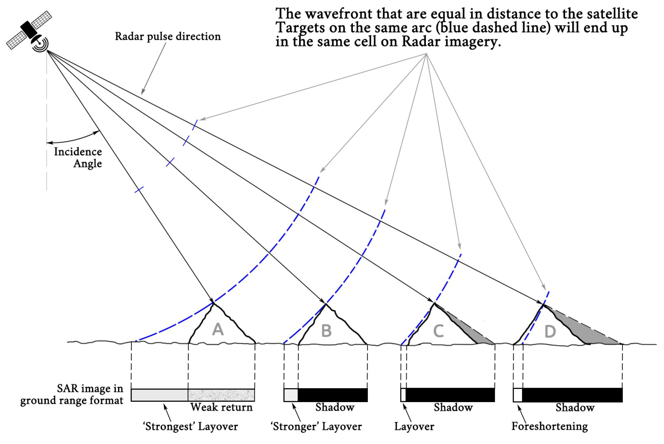
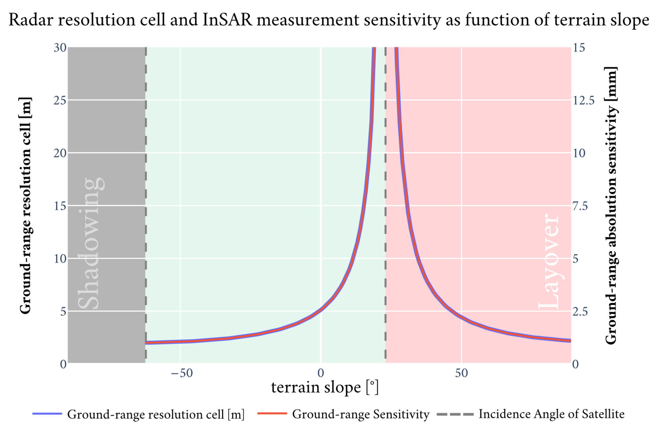
3.2. Geometric Distortion and Its Implication on InSAR

3.2.1. Why is Geometric Distortion Important for Monitoring Highway Slopes?

Geometric distortion [15] is part of the side-looking nature of the SAR satellite. The geometric distortion is a function of incidence angle, local topography (slope) and slant range resolution. Three common types of geometric distortion are illustrated in Figure 3, namely foreshortening, layover, and shadowing.
Geometric distortion is a particular concern for monitoring slopes. Figure 3 shows that the slope facing the satellite will be “squeezed" into fewer pixels in range direction SAR imagery, known as the foreshortening and layover effect. This also implies a lower spatial resolution for the satellite-facing side of the slope. The slope facing away from the satellite will have a better spatial resolution in theory, but depending on the steepness of the slope, the slope might either be completely shadowed by the mountain top (Figure 3) or give very weak return signals (Figure 4). Neither case is desired. For monitoring slope, we want to answer the three questions posed in Section 1, which is to give:
  • decent ground-range resolution;
  • decent sensitivity to movement in LOS direction;
  • decent backscattered signal, or equivalently, signal to noise ratio.
For a fixed terrain slope, the larger the difference between the incidence angle and the terrain slope (in range direction), the better the resolution and sensitivity (Figure 5) [15]. However, in terms of getting a good SNR for distributed scatterers, it is desired to have the inbound signal as orthogonal as possible to the surface of the slope (Figure 4) [17,18,19]. The final choice of the incidence angle should balance the SNR against the resolution.
Why do we need good SNR for InSAR results? It is because SNR is associated with InSAR measurement accuracy. The relationship between SNR and the dispersion of the displacement measurements along the line of sight (LoS) can be approximated as follows [20]:
σ L o S = λ 4 π · σ ϕ λ 4 π · 1 2 · SNR ,
where σ L o S is the dispersion of displacement along LoS, σ ϕ is the dispersion of phase, λ is the wavelength.

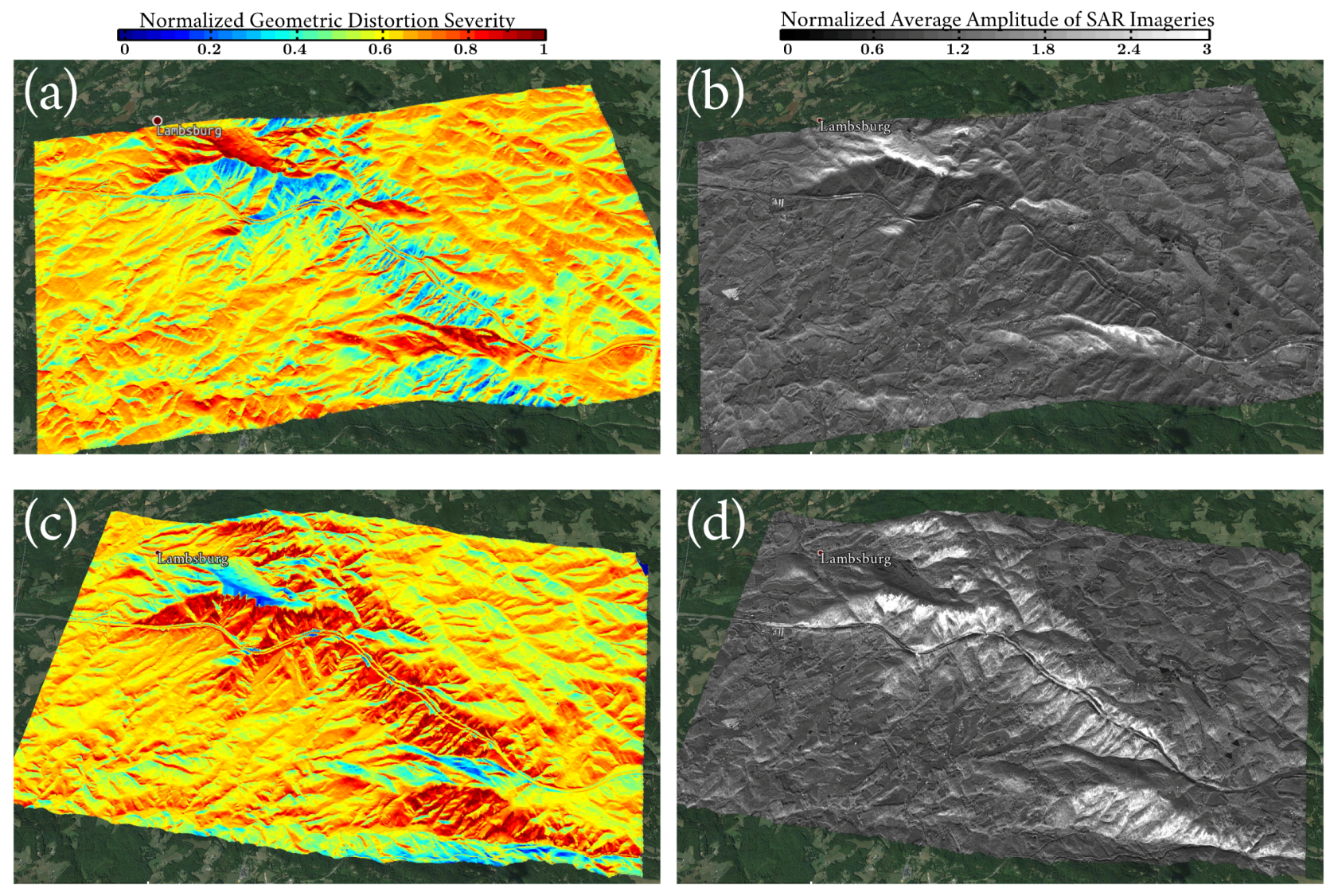
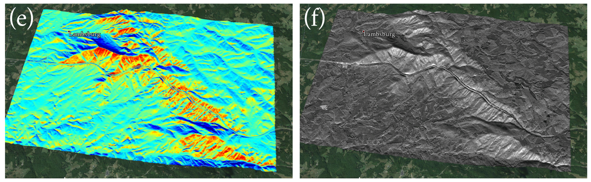
3.2.2. Simulation of Geometric Distortion

It is very useful to make a quick-and-simple simulation map of geometric distortion based on the available DEM and the incidence angle of the satellite. The simulation helped us better select the incidence angle to minimize the impact of geometric distortion for the given SoI [21,22]. According to Figure 3, the calculation on how much foreshortening and layover is easy, but calculating the shadowing area would be a little bit more complicated. However, for this project we would prefer the slope-facing track for guaranteeing enough SNR on the slope. Therefore, it is no longer necessary to precisely map the shadowing area. The following simple algorithm can thus be used for simulating the geometric distortion:
resampled_DEM = resample_from_latlon(DEM, resampled_coordinate=radar)
for line in resampled_DEM:
    for pixel in line:
     local_incidence_angle = incidence_angle - slope
normalized_local_incidence_angle = (90-local_incidence_angle) / 90
return normalized_local_incidence_angle
In this way, we simulate the geometric distortion by simply calculating the local incidence angle.

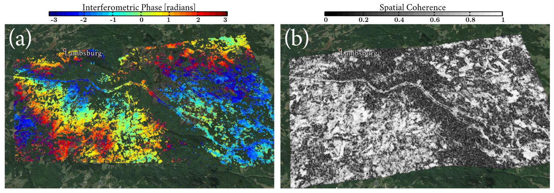
3.3. Quick Check with a Few Interferograms and Coherence Maps per Track

Interferogram and coherence map serves as a quick check before the MTInSAR processing. After the simulation of geometric distortion, and if the budget allows, it would be a nice-to-have to order a few pairs of SAR images per track. With real data we could check the following:
  • From the intensity map and coherence map, we could check the correctness of the simulated geometric distortion map;
  • From the interferogram and coherence map, we could check for the best coherence at the SoIs among all available options.

3.4. Multi-Temporal Time Series Analysis

After selecting the optimum satellite configuration, the MTInSAR will be performed. The method is already well discussed in [5] and will not be elaborated here. However, for this specific project, there are two steps that deviate from the classic algorithm that need to be elaborated on.

3.4.1. Ignore the Atmospheric Effect in a Small Area

It has been shown that the atmospheric phase screen (APS) is a long wavelength signal and has a decorrelation length of several hundred meters. We can assume its impact to be small in a relatively small area, say, a few hundred meters up to a kilometer, and neglect it [23]. Following this assumption, for a relatively small area, we would have the following:
Δ ϕ = Δ ϕ deformation + Δ ϕ height + Δ ϕ noise ,
where Δ ϕ is the double phase difference: the difference between the target and the reference pixel, the difference between the master and slave dates. When the atmosphere component is neglected, the problem becomes a simple optimization problem of finding the correct value of deformation and point height so that the noise level is minimized (temporal coherence is maximized) [23]:
deformation ^ , h ^ = arg max i = 1 N exp { j ( Δ ϕ Δ ϕ deformation Δ ϕ height ) } .
It should be mentioned here that deformation ^ is not necessarily the deformation rate. It could also be the deformation time series. If the expected movement can be well modeled by linearity, then we would have deformation ^ = v ^ · t . For non-linear movement, a non-parametric model could be used where no velocity is estimated (see Section 3.4.2 for details).
This optimization problem in Equation (4) does not necessarily converge, but we can define a search space to find the optimal solution. This is commonly referred to as the periodogram approach [7]. The maximized absolute value of the periodogram is usually referred to as the temporal coherence ( γ ) with respect to the reference:
γ = | 1 N i = 1 N exp { j ( Δ ϕ Δ ϕ deformation ^ Δ ϕ h ^ ) } | ,
where γ is a value between 0 and 1. 1 means that the model (estimated height and deformation) fits perfectly to the observed data and vice versa.
It should be noted that InSAR and MTInSAR are all relative measurements. Within each small area, we are measuring the relative deformation between each point and the selected reference point. For this purpose, the reference point should be stable. In this project, there is already a-prior information that the highway is in general stable. Hence, for each small area, we can select the reference point near the road and study the movement of the slopes with respect to this reference.

3.4.2. Non-Parametric Model for Non-Linear Movement

In the classic MTInSAR processing, the unwrapping of the points in time is done by assuming a parametric model in Equation (4). This assumption works great for motion that could be well modeled by a parametric model (i.e., linear, quadratic or seasonal), but for erratic behavior, this could lead to unwrapping errors and low level of confidence. A technique that could work well is a non-linear non-a-priori model. The non-a-priori model is done by estimate the low pass component using a five-samples temporal baseline weighted moving average and assume this residual phase term as an estimation of the non-linear motion contribution [24]. The non-linear model has been proved to work very well when there are adequate images that are sampled regularly in time [24].

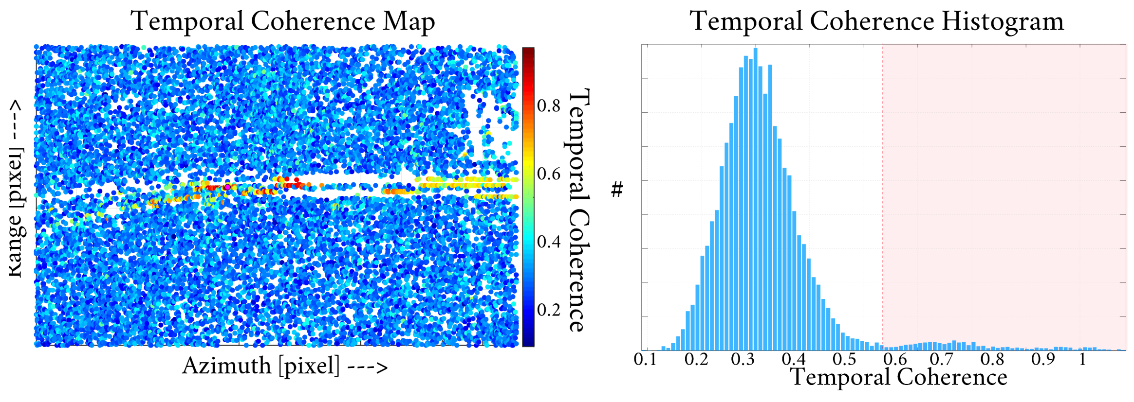
3.4.3. Selecting Temporal Coherence Threshold Value

After the MTInSAR process, we want to select only the points that are “informative”. Otsu’s thresholding method [25] is applied to this process.
First, we plot the histogram of temporal coherence for all points. With the presence of noisy points, the histogram would typically look bimodal, where the left “clutter” indicates the noisy points and the right “clutter” indicates the informative points. Otsu’s method finds the threshold that maximizes inter-class variance. An example is shown in Figure 6. In this example, the majority of points are noisy, but the bimodal shape in the histogram is explicit. In this project, the threshold is rounded up to the nearest 0.05.

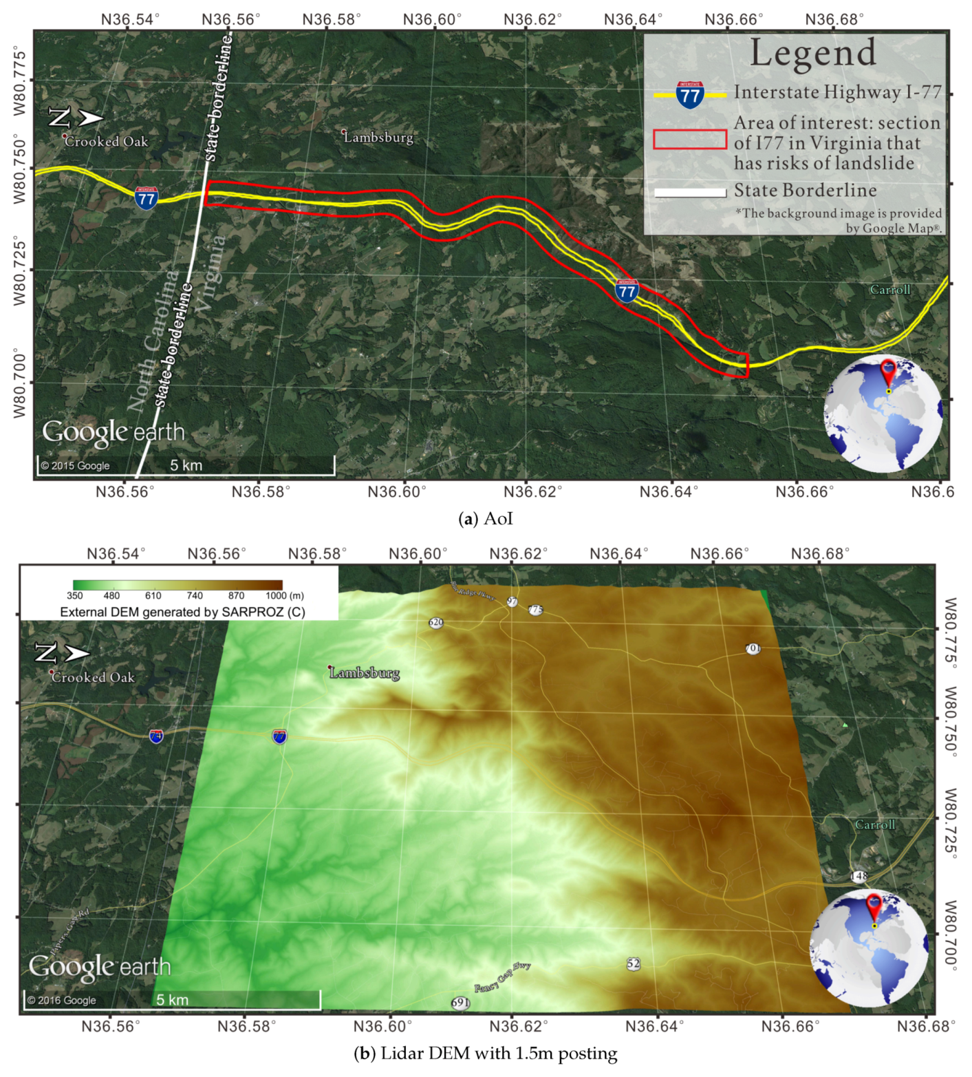
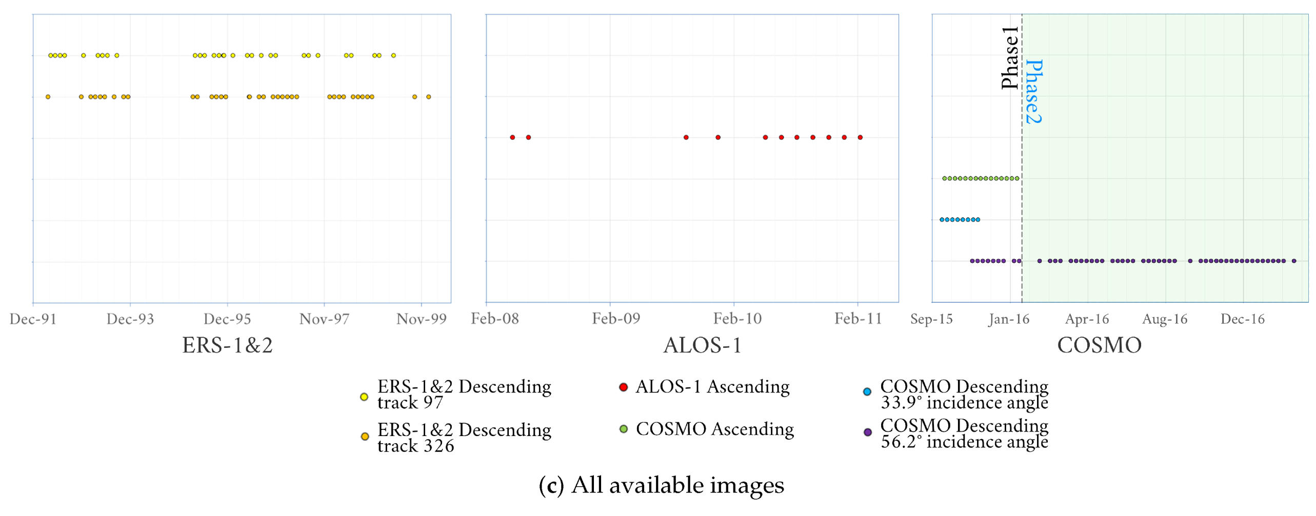
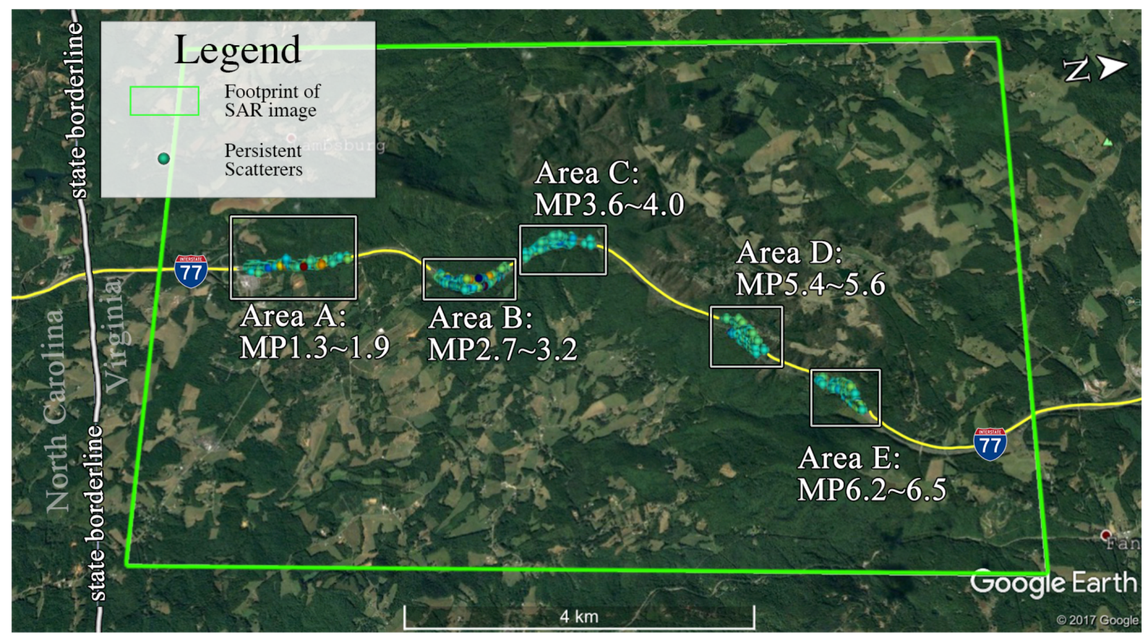
4. AoI and Available Images

The AoI is the section of US highway I-77 between milepost (MP) 0.0 and MP 8.0 in Carroll County, Virginia (VA). Due to dramatic changes in the terrain, numerous cut slopes were made along the road. The principal rock type is composed of metagraywacke. Since the geologic structure involves extensive faulting and complex folding, slope stability has long been a critical issue for past decades. Several slope instabilities have been reported over the years in this section. Therefore, VDOT has expended considerable resources dealing with the slope maintenance and remedial operations in this stretch [26,27].
The AOI is shown in Figure 7a. Our assessment focuses on the I-77’s slope as shown in the red box in Figure 7a, especially the slope to the west side of the highway since they are the ones that would pose risks to the road.
The local terrain height is obtained from a high resolution (1.5 m × 1.5 m) digital elevation model (DEM) (Figure 7b). The elevation of the I-77 increases from 450 m (MP 0.0) to 850 m (MP 8.0), with an average slope of 0.17:1. The steepest slope can reach 0.25:1 to 0.5:1. The slope orthogonal to the highway is between 0.2:1 to 0.5:1.
The available images that were used for this project are listed in Table 1.

5. Results

5.1. Phase 1: Analysis of Historical Data for Choosing the Best Configuration for the Monitoring Project

Phase 1 evaluated all the available images for choosing the best configuration. The evaluation focused on the performance of InSAR at the slopes of interests. The chosen configuration would have the least geometric distortion, meanwhile yielding a decent SNR. In this section, we show the cumulative change detection map, the geometric distortion simulation map, and a few interferograms. Based on the results we evaluate the best satellite and configuration for phase 2.

5.1.1. Intensity Change Map and Historical Landslide Locations

In this section, we show an example of the cumulative intensity change map from ERS-1&2 descending track 97. As shown in Figure 8, the cumulative change map provides intensity changes during the data acquisition period. Several locations with significant cumulative changes correspond well to historical landslides/rockfall locations. Even with the low spatial resolution and strong geometric distortion in ERS1&2 data, it is still possible to identify a number of locations of significant changes in the past. For ALOS-1, because of the limited number of available images, no significant change is observed.

5.1.2. Simulated Geometric Distortion Map and Intensity Map

This section shows the simulated geometric distortion map and the intensity map. The focus is on the slope on the west side of the highway. The first thing to notice is that the ascending pass does not have severe layover and foreshortening for our SoI (Figure 9a), but also we see relatively low backscatter there (Figure 9b). As for the descending passes, the larger incidence angle gives less geometric distortion. The intensity map at the SoI also supports the simulation results. The geocoded reflectivity map with the larger incidence angle also shows “finer details” (higher resolution) at the SoI. This corresponds well with Figure 5.
For choosing the best candidate, we rule out the ascending track first. The backscatter/SNR is too low at the SoI, and we risk getting the shadowing effect as well. Among the two descending tracks, the one with the larger incidence angle, 56.2 , gives less geometric distortion and better spatial resolution.

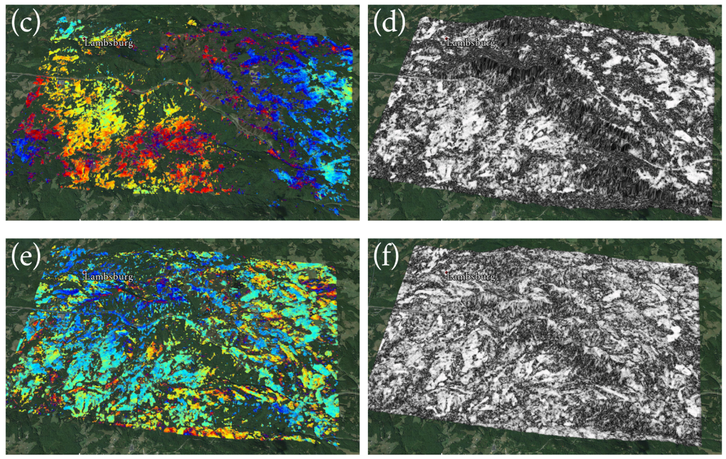
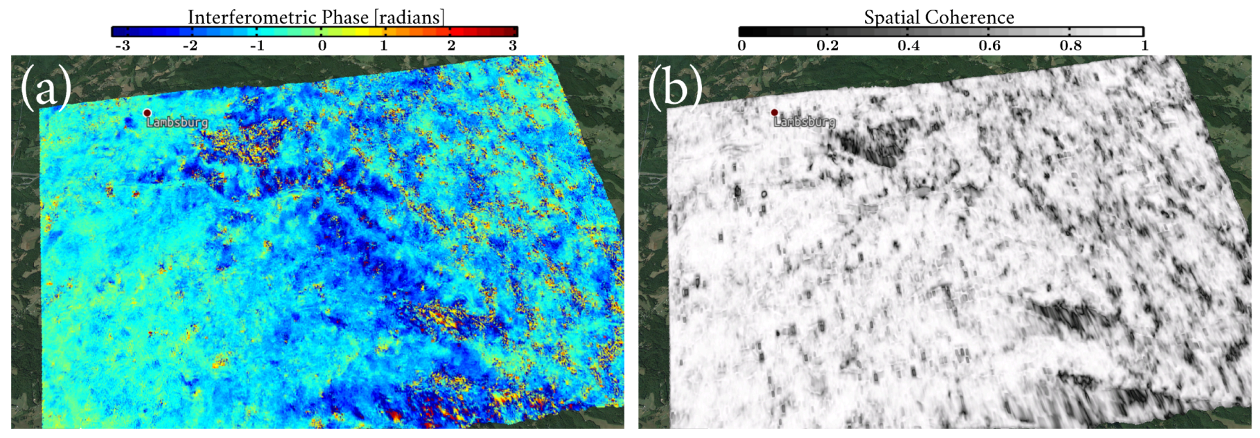
5.1.3. Interferograms and Coherence Maps

High Resolution X-band COSMO

Examples of interferograms and the corresponding coherence maps for COSMO are shown here. A coherence threshold of 0.6 is applied for plotting.
The descending track with the larger incidence angle gives the best result. The ascending track (Figure 10a) reveals the outline of the highway, but there is a very little coherent signal on the slopes, either due to the shadowing effect or low backscatter signal. The descending track with a 33.9 incidence angle (Figure 10c) shows neither coherence on the road nor on the slope, most likely due to the strong geometric distortion. This result agrees well with the previous inference from geometric distortion simulation.
It should be noted that there are more than one pair of interferogram available for each track by the end of phase 1. All of the interferogram pairs from an MST graph were processed. Only selected examples are included in this article. In addition, since the coherence of interferogram can be influenced by a lot of factors, we try to select interferograms with parameters as close as possible (i.e., spatial baseline, temporal baseline, time of the year, etc.) for comparison purposes. The exclusive conclusion is still to proceed with the descending track 56.2 incidence angle for getting the best coherence.

Alternative: L-band

Another option is L-band. As a matter of fact, since L-band performs much better than C and X band over vegetated areas, it should be the top candidate for this project. Figure 11 shows an example from ALOS-1 data. Even with a temporal baseline of 46 days and a spatial baseline of 675 m, the interferogram was highly coherent almost everywhere. Currently, ALOS-1 is no longer operative. The new generation, ALOS-2, has a better spatial resolution (3 m available) and a shorter revisit time (14 days). Based on the L-band signal characteristics and ALOS-2’s specifications, it should be the ideal candidate.

5.1.4. Assessment of Best Configuration

Now we have all elements to select the best configuration. We do so by reviewing the questions from the first chapter.
  • What is the most suitable wavelength? From the interferograms, it is clear that L-band gives the best coherence. C-band ERS data does not give coherent interferograms (and thus we did not show any in this article). For the X-band COSMO-SkyMed, the worst performances should be expected in terms of interferometric coherence. Surprisingly, the results in this work prove that, notwithstanding the properties of the terrain (vegetation and steep slopes), it is still possible to obtain coherent interferograms at certain locations, i.e., the highway and the bare-rock slopes. The reason for such performances is the high resolution and the very short revisit time of the COSMO constellation, where the shorter revisit time compensated for the temporal decorrelation effect.
    Nevertheless, another point to consider is that X-band is more sensitive to movement than L-band. When the expected deformation rate is at the scale of a few millimeters per year, then X-band would be more sensitive to such movement than L-band.
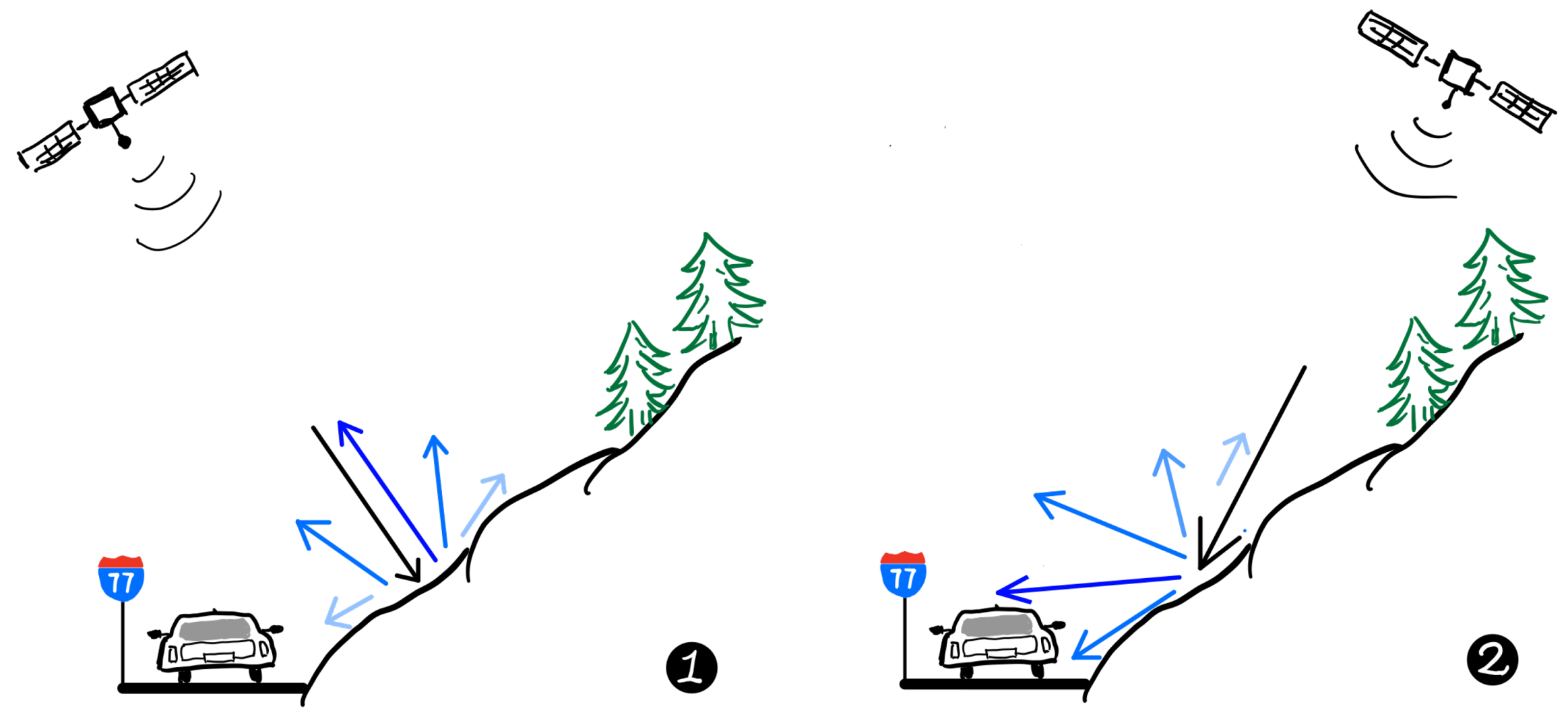
  • What is the best option for the incidence angle? Based on simulations, it is clear that the descending orbit with 56.2 degrees incidence angle yields the slightest geometric distortion among all the descending tracks.
  • What is a suitable revisit frequency? The coherence decay exponentially to revisit time [28]. L-band gives more coherence over vegetated areas, thus a longer revisit time could be accepted, i.e., 40 days or even longer. As for X-band, a much shorter revisit time is required to account for the temporal decorrelation. Based on the available interferograms, a suitable revisit time for the X-band should be much shorter than L-band. In this case, an 8-day-revisit-time for COSMO is proposed.
  • Should one use ascending or descending data? In the comparison between COSMO descending and ascending, It is then clear that the descending track should be selected for giving higher SNR and coherence on the SoIs.
  • What spatial/geolocalization resolution can be accepted for this project? This project monitors highways and the slopes. The scales of the two kinds are usually just a few meters to a few hundred. This means that the resolution should be at the scale of a few meters to give a sufficient number of points over the targets of interest. Out of all available dataset, the X-band high-resolution satellite (COSMO and TerraSAR-X) have the 3 m resolution, and the L-band ALOS-2 have the 3 to 10 m resolution.
  • What approach should be used for processing? The ideal approach is the persistent scatterers approach. SBaS approach usually does a spatial multilook and filtering [8], hence downgrading the spatial resolution of the final result. PS approach, on the other hand, does not trade SNR for spatial resolution. This project already monitors very small areas, hence a spatial resolution downgrade is not recommended.
To summarize, the best candidate for the next phase would be L-band, descending track with a relatively large incidence angle (i.e., 50 ), 3-m-resolution and 28-days revisit time preferred (or even 40+ days could do). ALOS-2 is the only one that could satisfy all the requirements with its stripmap ultra-fine (SM1) mode [29]. The runner-up would be COSMO or TerraSAR-X (the two have very similar specifications), also descending track with 3-m-resolution, 10-days revisit time or better. The shorter revisit time compensates for the temporal decorrelation.
We ended up selecting the COSMO purely due to budget consideration. The final configuration is COSMO descending track, stripmap mode, with 56.2 degrees incidence angle and 8-days revisit time.

5.2. Phase 2: Multi-Temporal InSAR process

This section shows the MTInSAR results. The entire AoI from MP0.0 to MP8.0 is divided into five smaller areas. Each small area includes a slope with bare rocks or soil that poses a potential hazard. Areas are selected based on past incidents. Figure 12 shows the location and size of each small area. In the following sections, they are referred to as small areas A, B, C, D and E.

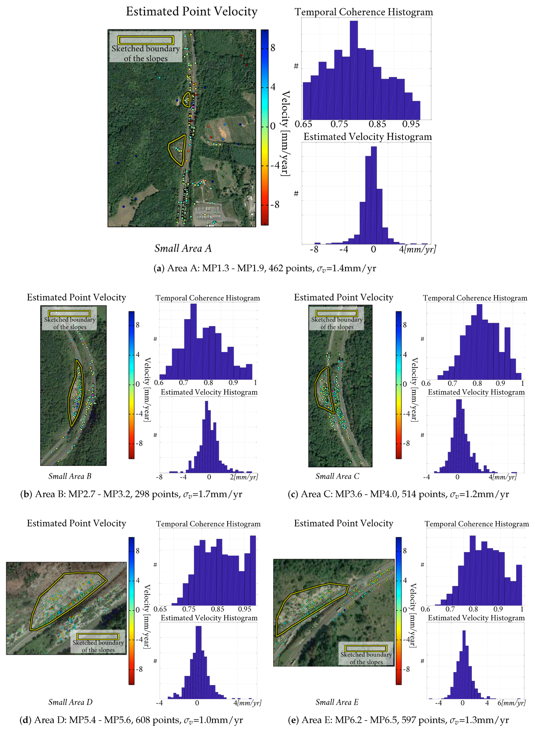
5.2.1. Overview of Small Areas

We start with an overview of all five small areas. Figure 13 reports three products for each small area: the estimated velocity map, the temporal coherence histogram, and the estimated velocity histogram. The estimated velocity standard deviation ( σ v ) also comes along with the histogram. The standard deviation is a good indicator of whether the estimated velocity of an individual point is statistically significant or not. For example, it would be worth checking points with an estimated velocity greater than two times the standard deviation (95% confidence level).
Figure 13 shows that the five small areas are overall stable. Around 95% of the points have a rate of less than 3mm/year along LoS (two times σ v ). For the most part, no signs of significant regional deformation could be observed on any of the slopes. There are some points on the slopes showing significant velocities, but these are mostly isolated cases, which means either the impact range is very small (just affecting a couple of meters) or the points are pure noise.

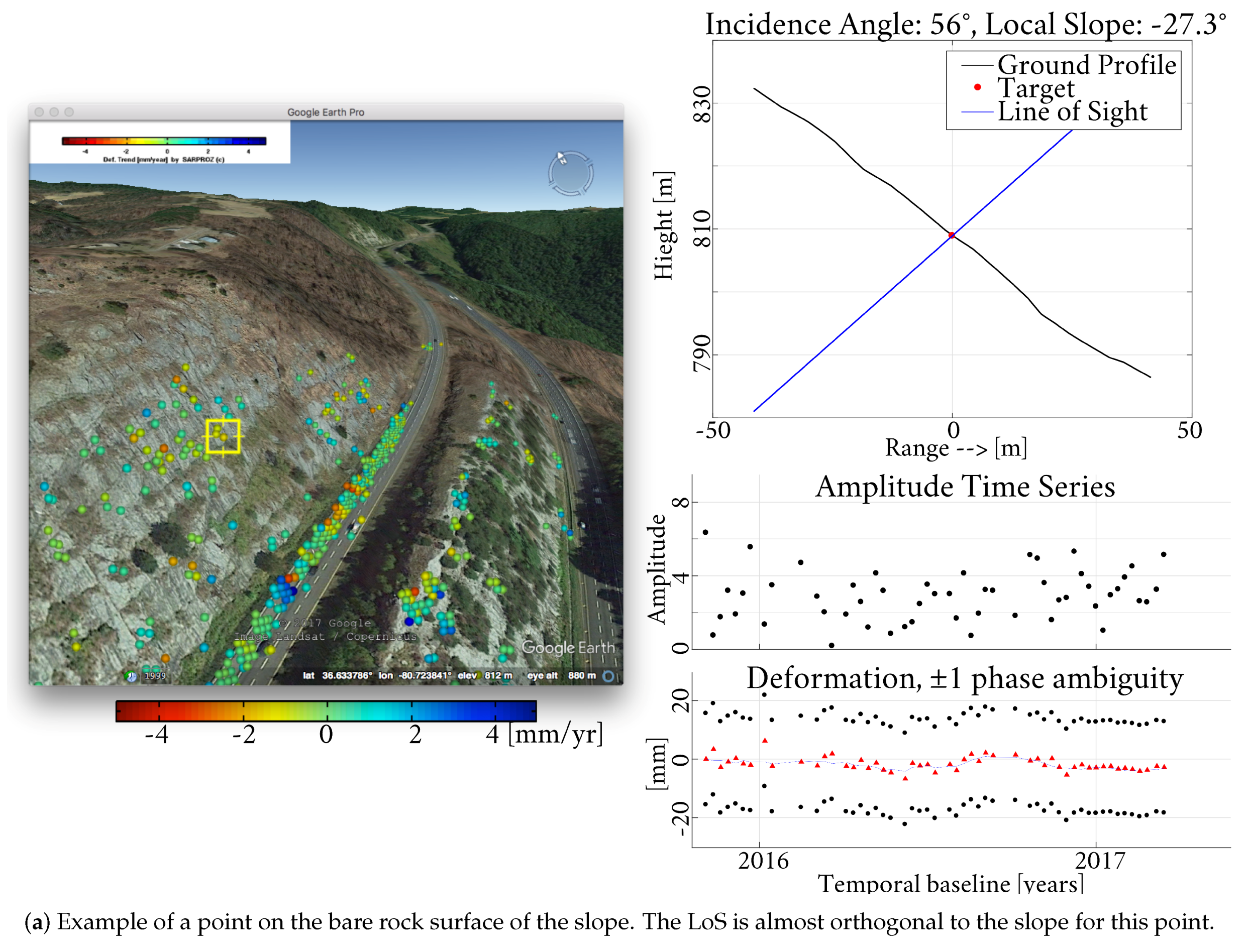
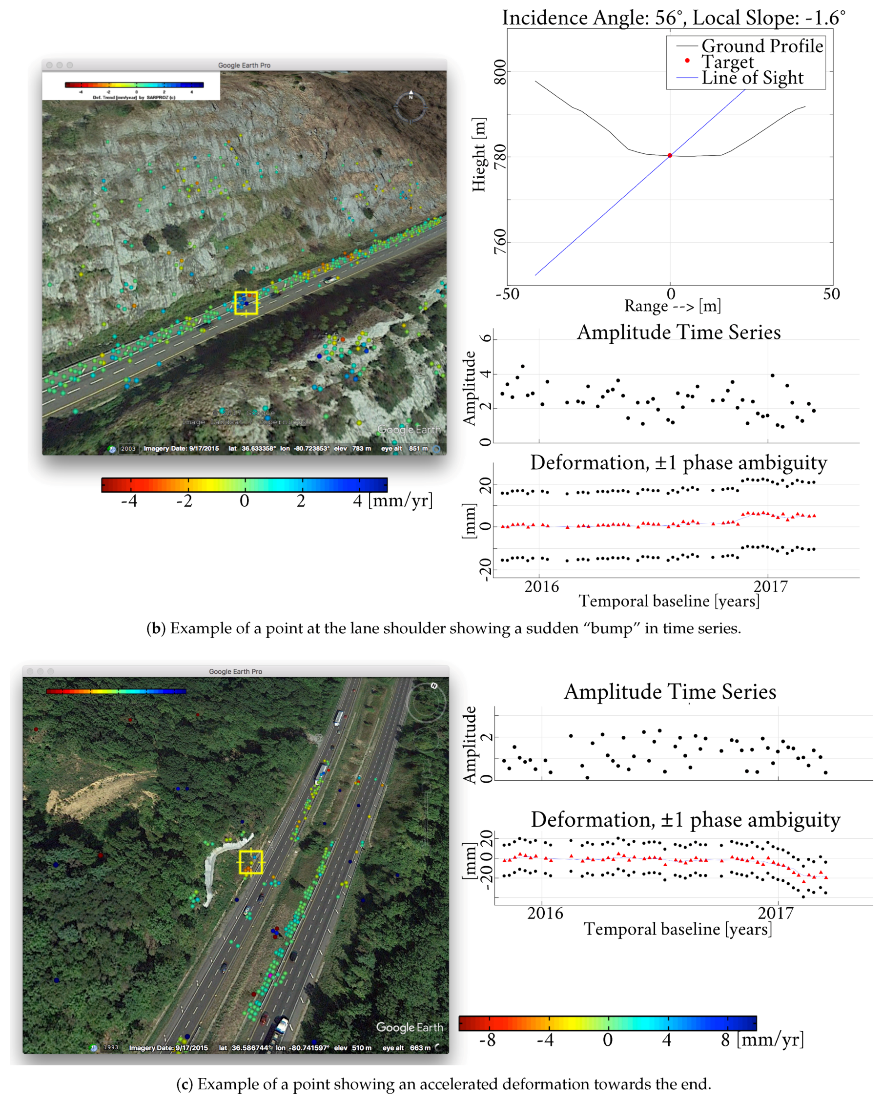
5.2.2. Some Representative PS Examples

This section shows four representative examples.
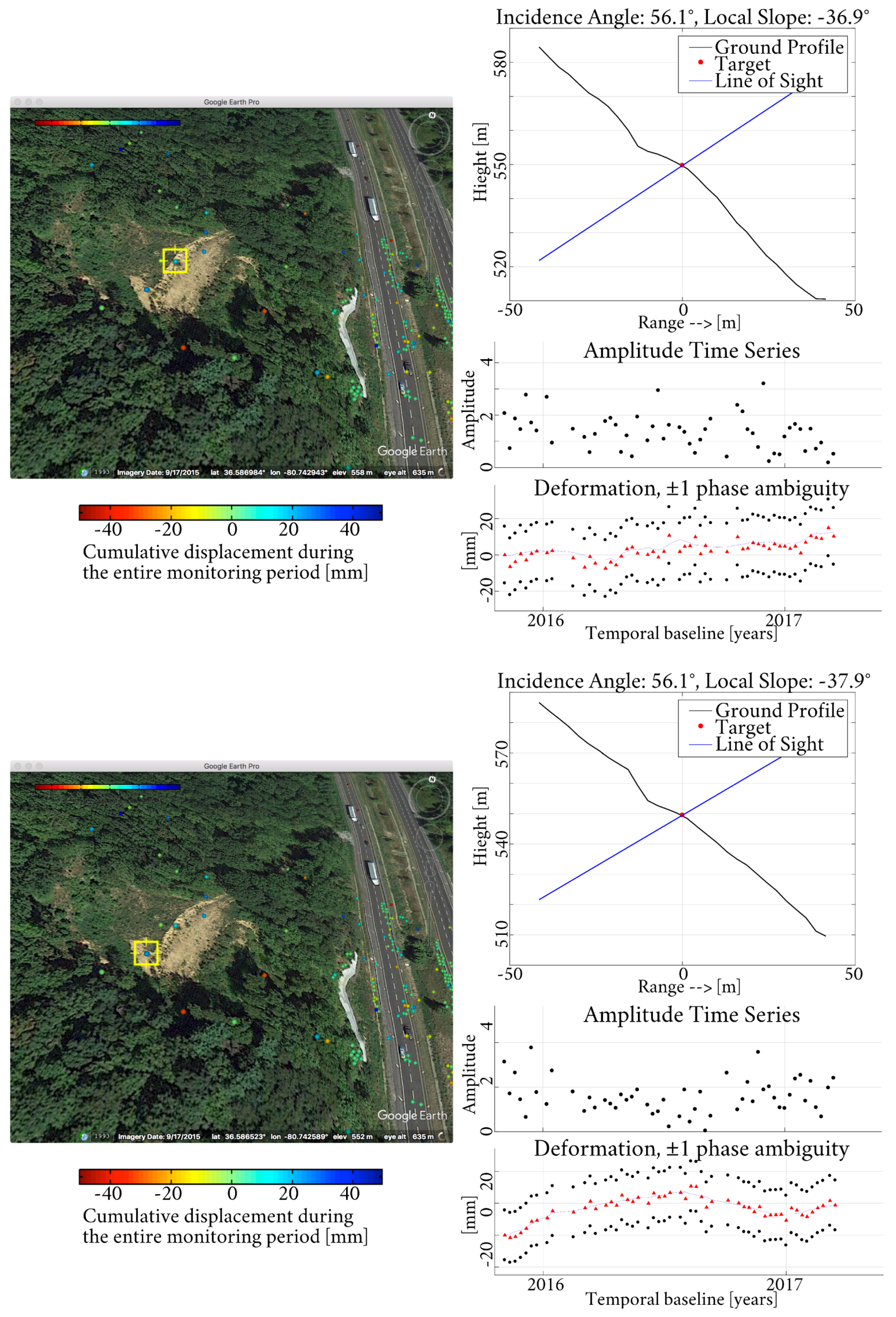
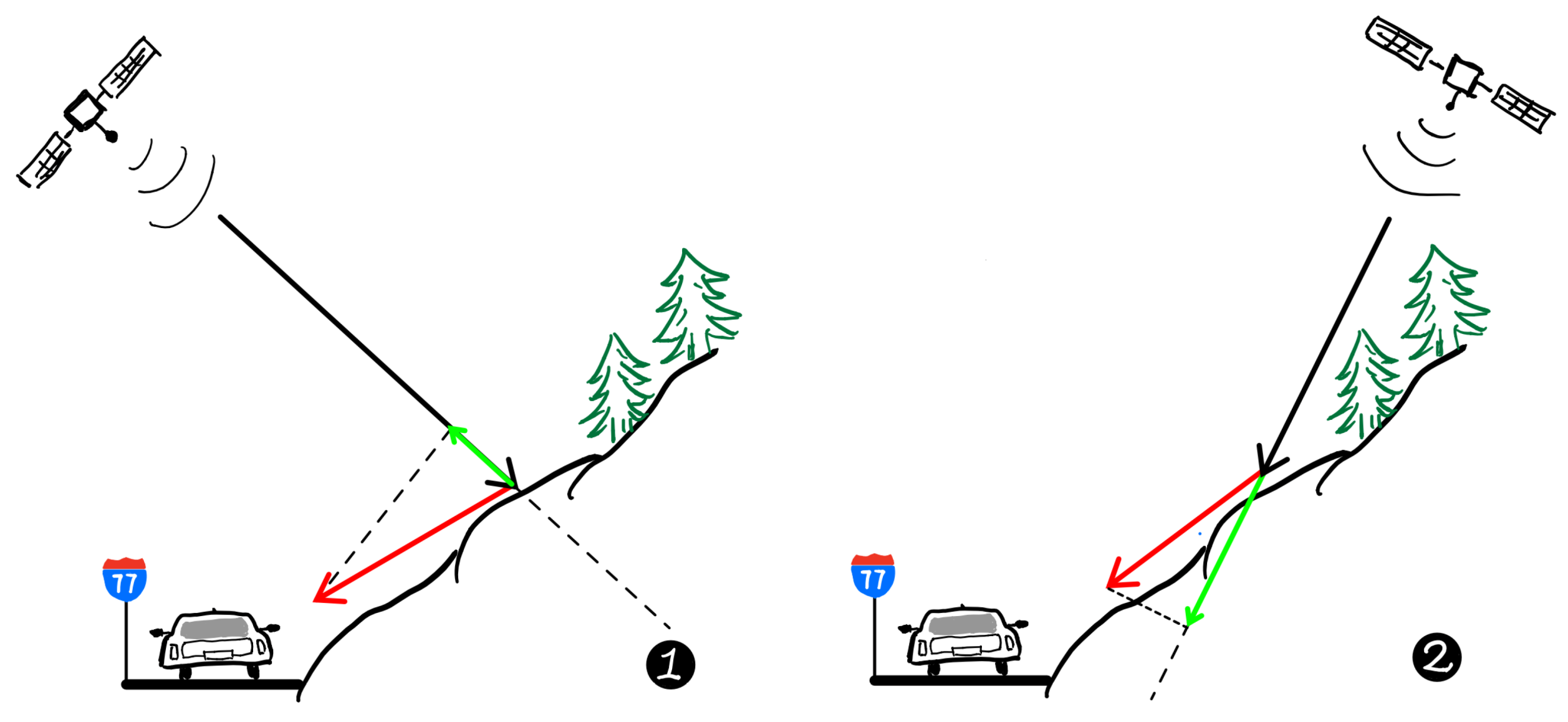
  • The first point in Figure 14a is located on the slope and appears to be stable along LoS. However, the upper right part of Figure 14a shows that the LoS direction is almost orthogonal to the slope, inferring that the selected geometry is insensitive to any settlement along the slope. While we chose an incidence angle to avoid geometric distortion as much as possible, it was hard to avoid geometric distortion everywhere.
  • The second point in Figure 14b is located at the foot of the hill. This point shows a sudden “bump” in time series but remains stable before and after the bump.
  • The third point in Figure 15c is also located at the foot of the hill. Thanks to the non-linear approach mentioned in Section 3.4.2, we are able to detect such non-linear movement of the point. According to the field survey, this acceleration towards the end of the monitoring period is likely to be caused by the cracks in the concrete ditch. The cracks may be associated with some movement at the toe of the slope, or they may be caused by water erosion of surface soils.
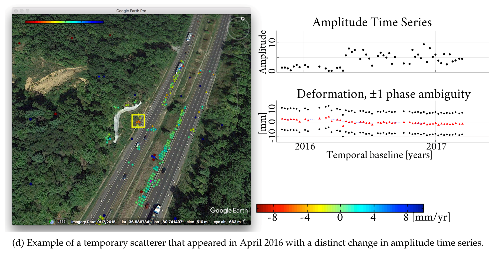
  • The last example in Figure 15d is a temporary scatterer that existed for only part of the monitoring period. A distinct change in amplitude time series is the characteristic of such temporary scatterers.

6. Interpretation and Field Works

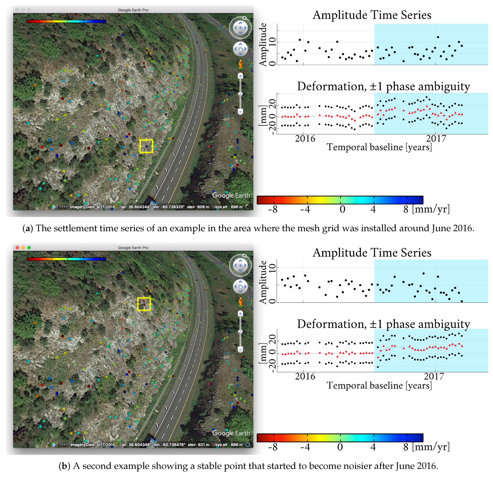
6.1. Case Study 1: Metal Mesh Installation Seen from InSAR

A number of points in area B exhibited similar behavior in their time series: very stable before June 2016, much noisier afterward. It turns out that a metal mesh was draped over the slope around June 2016 [30]. The entire rock face was protected with the steel wire mesh (secured with rock bolts) to prevent rocks from falling on the highway below.
Could the signal we see in Figure 15 originate from the installment of metallic mesh? Theoretically, the metallic mesh (typically a thin metallic grid) should not alter the SAR signal much, because radar signal should be able to penetrate the mesh grid (wavelength of X band is 31mm, while the size of the holes on the mesh should be at least a few decimeters). However, the process of installing the metallic mesh could interact with the local environment and subsequently cause some changes to the slope that is captured by SAR. The two examples in Figure 15e,f are likely the records of such sudden movement related to the mesh installment in June 2016. Specifically, both examples show a steady phase time series untill June 2016, followed by much noisier signals afterward. A few other points also show similar change patterns.

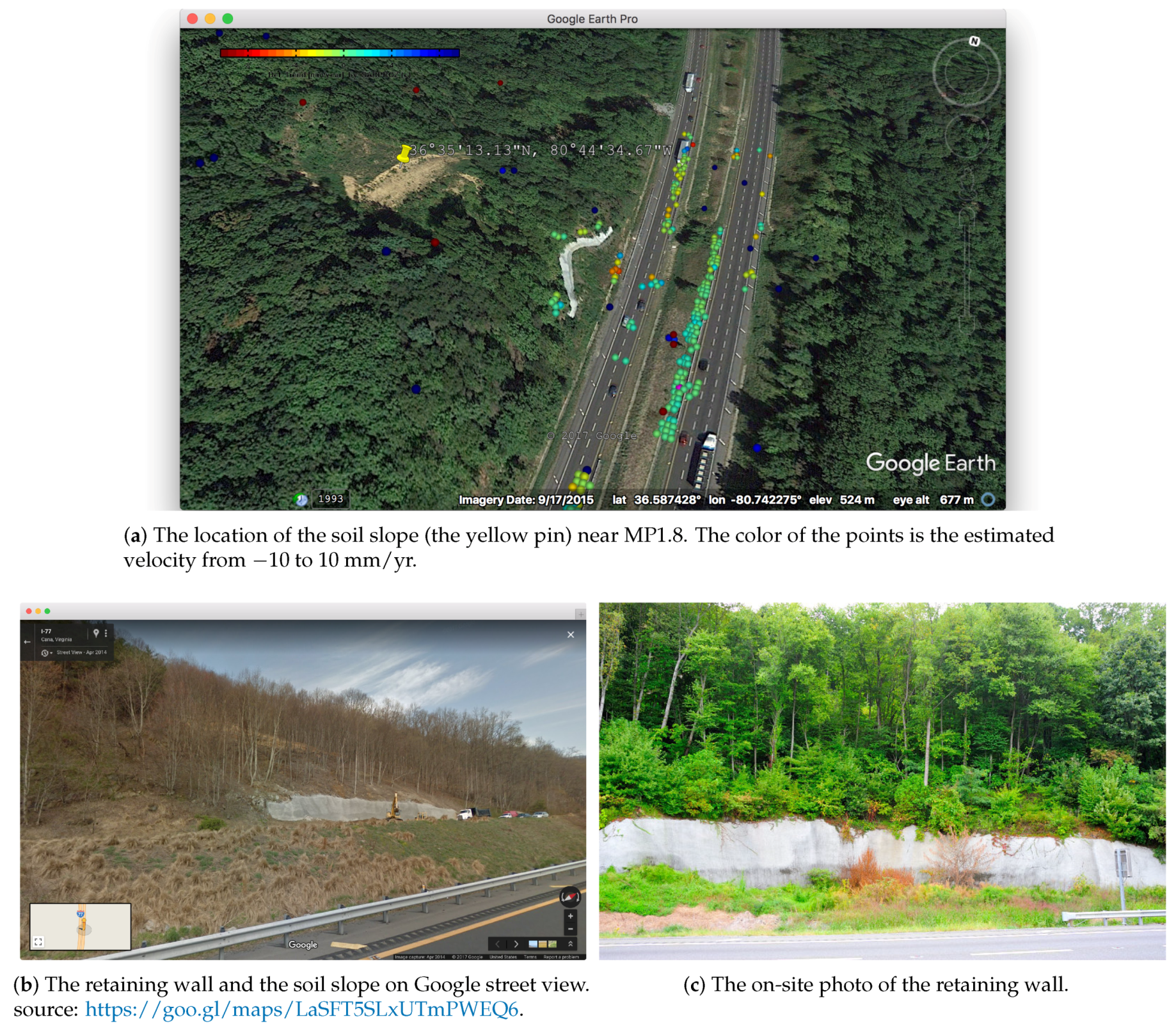
6.2. Case Study 2: The Soil Slope and the Retaining Wall at MP1.8 in Area A

6.2.1. The Slope at MP1.8

Particular attention is given to the slope located at MP1.8 of I-77. The attention is due to a known past movement also being monitored by the in-situ inclinometer. Reference shows an uplift from 0.5 inches (1.27 cm) to 4 inches (10.16 cm) over the past three years. VDOT has also taken action to build a retaining wall right underneath the soil slope. In this case study we want to explore if movements at this location could be picked up by the SAR satellite.
A soil slope is not an optimal observing target for InSAR, especially for shorter wavelengths such as the X band. Apart from the fact that the X band has a worse penetration over vegetation and soil, X band is also more sensitive to small movement than L band, which is not favored for this specific case.
To account for any non-linear movement on the soil slope, we applied the non-parametric model mentioned in Section 3.4.2. For this specific case, a window size larger than the default was used because the area is noisier. With this extra smoothing operation, we extracted a few more points on the slope showing trends of movement with a satisfactory temporal coherence value. A few examples are shown in Figure 16. Nevertheless, it should be pointed out again that phase time series have 2 π ambiguity, and the blue solid line representing the estimated time series is just the most likely trend out of all possibilities.
The examples reported here still show more complex movements and are still noisier despite the extra smoothing. In addition, no groups of points showing homogeneous behavior in time series could be found on this slope. The reported points with high coherence are more or less all isolated. In conclusion, due to the physical characteristics of the interaction between microwave and soil land, this slope appears noisy on SAR images. With an extra smooth filter, we could output a few points with good temporal coherence, but no conclusive information about the slope movement could be obtained.

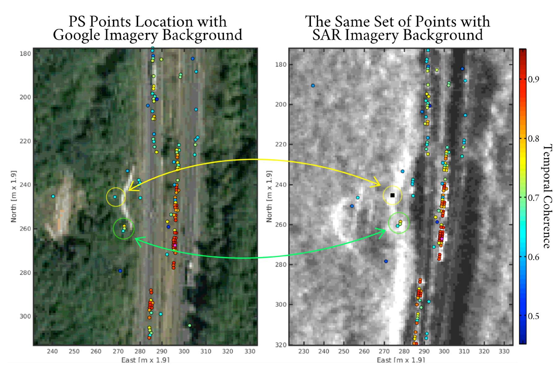
6.2.2. How Good Is the Geolocalization of the Points?

It is informative to study the stability of the retaining wall right beneath the soil slope. If the retaining wall is moving then the soil slope above may also be moving. This is why it is important to determine the stability of the retaining wall. To start with, in Figure 17a we notice some points just outside the white retaining wall on Google Earth imagery. We want to understand if these points should actually be on the retaining wall or not. If they are on the retaining wall, why are the geolocalization of these points wrong?
In general, the geolocation accuracy of InSAR points is better than the pixel resolution. However, a lot of factors could give a slight offset in the geolocalization, i.e., geometric distortion, side-lobes effect, multiple path effect and etc. In this case, by checking the location of PS points on SAR imagery, we could infer that the points near the white wall on Google Earth imagery actually belong to the white wall.
Figure 18 shows the points with Google Earth imagery and SAR imagery as the backgrounds. On the SAR imagery, we could see that the points are located in the “bright stripe", which clearly comes from the white retaining wall that is reflecting a significant portion of the radar signal and is much brighter than its surroundings on SAR imagery. The slight location mismatch of the wall between Google Earth imagery and SAR imagery is most likely the result of the strong geometric distortion of SAR imagery.

7. Discussion

7.1. How to Better Monitor the Slopes?

7.1.1. The Relationship between the Estimated Velocity and the Local Slope

InSAR measures the ground movement projected in the LoS direction. For the radar system, there are two implications stemming from this geometry.
In the first place, since radar satellite flies in sun-synchronous polar orbits, around 10 degrees off north-south direction, then any North–South movement will hardly get projected on to LoS direction. Depending on the incidence angle, the majority contribution to LoS measurement would be east-west and vertical movement.
The second point relates to how radar satellite captures the movement of unstable slopes. One assumption is that the surface would slide down along the slope due to the gravitational force. Figure 19 depicts this hypothesis. When the satellite is facing away from the slope, the unstable surface would move away from the satellite. However, when the satellite is facing the slope, depending on the steepness of the slope, the unstable surface would either move towards or move away from the satellite. In the worst case where LoS is orthogonal to the slope, then the projection would be close to zero meaning the satellite would not be able to capture the ground surface movement along the slope. Figure 19-1 shows a case where the surface of the slope is moving towards the satellite along the LoS direction as it slides down the hill. Understanding this mechanism helps to interpret the results.

7.1.2. A Possible Scheme for Soil Slope Monitoring: Installing Corner Reflectors

The physical characteristics of the interaction between the microwaves and the soil determine that the signal of movement will be dominated by the noise. Advanced processing techniques might suppress the noise, but when it exceeds a certain level, the information could no longer be extracted. A feasible solution for monitoring slopes of such kind is to install corner reflectors.
Corner reflector is a man-made strong scatterer that often shows very high signal to noise ratio on SAR images. A reflector is usually made of two or three metallic plates that are mutually perpendicular to each other and will reflect signals back directly towards the source. Corner reflectors are easily manufactured, cost-effective and easy to install. For the purpose of slope monitoring, corner reflectors could be mounted at various locations on the slope surface. Once installed, they would serve as persistent scatterers on SAR images. As long as the path from the satellite to the reflectors is not blocked, the phase time series could be derived.
The technique is easy to implement and works especially well for complex ground features. The reflector is robust against noisy ground features such as vegetation and soil. This technique is very mature and has already been well applied to a number of monitoring applications [3,4].

7.1.3. How to Improve the Soil Slope Monitoring Result from the Algorithm Side: A Comparison with Other State of Art Processing Techniques

Another important issue is how to improve the monitoring result purely from the algorithms point of view. The PSI method we have been using in this study is designed to work better with strong reflectance scatterers such as persistent scatterers. But for distributed scatterers [31] that do not have a dominant reflectance signal, the SNR will be much lower and the PSI will be adversely affected.
To overcome this spatial decorrelation effect of distributed scatterers, there are two other options parallel to the PSI approach. Both options consider the spatial dependency of neighborhood pixels in their processing. The first approach is the small baseline subset (SBaS) [8]. The other approach is the “distributed scatterers” (DS) processing, or sometimes referred to as the hybrid methods. The DS method shares a very similar idea with SBaS in the sense that it also does “spatial filtering” (but sometimes in a more complicated way, i.e., recalculate the equivalent single master phase (ESM) with maximum likelihood estimator (MLE) [32]). Unlike SBaS, the hybrid method takes advantage of results from the PSI processing (i.e., usually the DS is unwrapped with respect to the nearest PS point [32]). There are a few deviations from the hybrid method but they all share a similar idea: to group neighborhood pixels with “similar behaviors” for canceling out the noise in each individual pixels and hence to increase the SNR. In addition, the QPS [33] method can be also counted as a hybrid method since it shares some similarities with both the SBaS technique and the PSI technique. In conclusion, the SBaS/hybrid method trades spatial resolution for measurement accuracy (or equivalently, SNR) and coverage. The smoothing operation in space will likely yield more DS points that give higher SNR but at the cost of lowering the spatial resolution.
For this project, since the PSI result on the soil slope is still rather noisy, a possible alternative might be the SBaS or the hybrid method. The biggest challenge with this soil slope, however, is the size of the soil slope. It could be seen from Google Earth that the size of the slope is at most 50 by 20 m. With the 3 m COSMO data, if a multilook window of 10 is used for SBaS or for the DS method, the entire slope would only be 1 pixel in size. Time series derived from only 1 pixel would not be enough to draw a sound conclusion. If we have to monitor a bigger area, then the SBaS/DS might be a better choice.
One other option to consider in the PSI processing is to add more models in the estimation of the periodogram [34]. There is usually a causal relationship between the settlement of soil and moisture content or temperature [35]. This implies that one can add precipitation model and/or temperature model in the PSI processing. Models with more dimensions (i.e., linear and seasonal) usually give a better fit and could reveal more information on points’ movement. On the other hand, there is always a risk in creating a more complex model.

7.2. Limitations and Applicability of InSAR Data for Slope Monitoring

7.2.1. One Size Cannot Fit All!

In phase 1, we tried to select a globally optimal configuration for slope monitoring. For example, we have chosen a large incidence angle to avoid the overall geometric distortion. And we selected the X band for its high resolution and sensitivity to small-scale settlement. However, later on, we’ve seen a few examples for which the selected configuration is not ideal. For example, the larger incidence angle gives the strongest geometric distortion for the point in Figure 14a; or the X-band does not reveal coherent points on the soil slope at MP1.8 (Section 6.2). In conclusion, there might not be an “optimal configuration” that could work well for every location in the AoI.
There are two ways to tackle the issue. The first is to apply different processing methodology accordingly. For example, Section 6.2 mentioned using a larger filter window for locations with more noise. The second way is to use different datasets. For example, to deal with the decorrelation of the soil slope, we could have used the L-band data. If the budget allows, it would always be better to monitor with multiple tracks or multiple satellites. In conclusion, for complex monitoring cases, there might not be a “one-size-fits-all” satellite configuration that works everywhere. We tried to select the configuration that is at least optimal for the majority part of the AoI, and then improve the results with contextual background and adaptive processing algorithms.

7.2.2. Comparison of InSAR and LiDAR for Deformation Monitoring

Another important assessment is to compare InSAR and the other very popular and widely-used monitoring technique, Light Detection and Ranging, also known as Laser Scanning (LiDAR). Both LiDAR and InSAR are active measurement techniques. They both transmit pulses of electromagnetic waves and record the resulting echo to get target information. While both techniques are capable of performing the same task, LiDAR is often deployed for generating the Digital Terrain Model (DTM), and InSAR is typically used for detecting ground movement. This difference in applications stems from the underlying principles of the two techniques. InSAR derives ground surface motion by measuring the phase difference between successive radar signal acquisitions. InSAR system sensitivity to detecting ground movement is range independent and proportional to signal wavelength, typically capable of delivering millimeter range accuracy of measurements. However, its sensitivity in deriving ground height is inversely proportional to the satellite spatial baseline, which normally translates into a meter level accuracy.
The LiDAR sensor is a time-of-flight system that collects 3D coordinates of targets based on accurately measuring the laser signal travel time. LiDAR may be the best choice for 3D reconstruction, however, it is harder for monitoring projects because it is practically impossible to reconstruct the same point cloud in space. LiDAR change detection is achieved by creating a 3D model from the point cloud using a triangular grid and then comparing the grids. Hence, the accuracy of change detection depends on the point cloud density, which is range dependent. Ground-based LiDAR can typically achieve an accuracy of approximately 1.5 cm up to maximum distances of about 800 to 1000 m [36].
These two techniques face similar challenges when measuring deformations, as follows [37]:
  • Optimal geometry for measurement. While LiDAR and InSAR use different acquisition geometries, they require optimal geometry for specific targets. A bad geometry in InSAR results in a geometric distortion on the SAR image, while in LiDAR it leads to insufficient return signal for successful measurement.
  • Processing of massive volumes of data and development of a fully automated deformation analysis method. Both techniques require processing massive amounts of data. The problem is to extract useful information and to develop an effective automated process for decision making.
  • Sensitivity to land cover. Both systems tackle this problem differently. X-band radar requires larger patches of unobstructed ground and cannot penetrate tree canopies. LiDAR’s very narrow laser beam is usually more effective in penetrating vegetation, but extensive signal processing is still required.
When applied to deformation measurements, InSAR offers the following advantages over LiDAR, as follows:
  • Independent from most weather conditions;
  • Day/night measurement capability;
  • No fieldwork required (this does not apply to ground-based InSAR though);
  • Consistent satellite revisit times, typically every 8 to 11 days;
  • Wide area coverage at any location on Earth. LiDAR provides point clouds over a relatively small area, while InSAR can provide a spatially complete map of ground deformations with millimeter to centimeter range accuracy. Typical coverage of one SAR image is on the order of 50 to 100 km square or rectangular. This approach allows for analyzing wide-area deformations. Moreover, with the InSAR technique, it is possible to detect displacements at locations where they are not anticipated, unlike in the case of geodetic techniques where (because of costs) measurements are performed only at locations suspected of undergoing deformations. When comparing the cost per unit area, InSAR can offer a more economical option when wide-area monitoring is required;
  • High measurement accuracy. With the correct configuration, InSAR can reach a millimeter level accuracy, which is significantly better than airborne LiDAR systems, and most of the long-range and medium-range ground-based laser scanners. Significantly, the accuracy of InSAR technique is independent of the distance between the SAR satellite and the ground target;
  • Access to historical data, allowing the analysis of past displacements. This capability is available with some radar satellites.
Among the significant limitations of space-borne InSAR technique for monitoring purpose are the following:
  • InSAR data processing is more complex than LiDAR. Even though this technology is relatively well developed and the processing algorithms are very robust, it requires experienced personnel and sophisticated software to process and interpret data correctly;
  • Signal phase ambiguity. The measured displacements are usually ambiguous because the phase is always wrapped between 0 and 2 π . The problem can be partially solved by the PSI method but only subject to certain assumptions;
  • Resolution. There are some limitations of space-borne satellite SAR systems, including low temporal and spatial resolution and the inability of real-time monitoring. Currently, one way to overcome this limitation is by using a ground-based SAR system.

7.3. Next Step: More Satellites, Lower Costs

Currently, the bottleneck of InSAR monitoring is not the theoretical limitation of the InSAR system, but is rather the available datasets at a reasonable cost. For example, this study eventually turned down the 3-m-resolution L-band data with 14 days baseline simply due to budget limitation. Based on the assessment from archived data, it is almost certain that the L-band ALOS-2 data would give a much better result. Some of the other limitations, such as the signal phase ambiguity and resolution, could also be addressed with more operational satellites, shorter temporal baseline and higher spatial resolution (i.e., higher bandwidth or spotlight mode).
It is encouraging to witness the success of Sentinel-1A/B system and the amazingly rich data archives all over the world have already boosted InSAR applications. As we head into 2020, there are solid opportunities from both government agencies and commercial cooperations. From the government agencies’ side, the mainstream satellites including TerraSAR-X, COSMO-SkyMed, and RADARSAT have all seen the launch of their next generations, including PAZ, COSMO-SkyMed Second Generation satellite (CSG1) and RADARSAT Constellation Mission (RCM). The L-band ALOS-4 and NISAR are scheduled to launch soon. From the commercial side, a number of start-ups have been working on microsatellites. The microsatellite constellation aims at providing images with very high revisit frequency at much lower costs. Both Iceye from Finland and Capella Space from the U.S.A. have successfully launched their pilot satellites for a proof-of-concept. Iceye has started providing commercial services, and Capella Space will start commercial operations in 2020.
If we plan to perform a similar study in the next few years, we would foresee more choices of data sources, more availability of data, better temporal/spatial resolution and much better overall results.

8. Conclusions

In this study, we attempted to explore comprehensive solution to a highway slope monitoring project. Two phases were carried out for the study. The first phase determined the most suitable satellite and configuration for a planned monitoring project. The second phase carried out the MTInSAR process and explored the slope movement along the highway.
For the first phase, the simulated geometric distortion map, cumulative change detection map, intensity map, interferograms and coherence maps were generated from all available historical images. By inspecting the end product, both the satellite and the configuration that gave the best coherence and least geometric distortion in our AoI were selected. The best candidate for the monitoring project would be ALOS-2 descending track, and the runner-up is COSMO descending with 8-days-revisit-time. We ended up using COSMO by considering the available budget.
For the second phase, the MTInSAR process was carried out. A total of 52 X-band COSMO images spanning almost one and a half years were used for the analysis. The entire project area was divided into five smaller areas, and for each small AOI, the PSI method was used for estimating the displacement and height of persistent scatterers. PS points with relatively high temporal coherence were closely examined. Locations showing evidence of movement were reported, and a fieldwork was carried out for interpretation and validation. Finally, we arrived at the following conclusions:
  • Persistent Scatterer Interferometry can be used to monitor slope deformations. Analysis of spaceborne X-band data indicates that rock slopes can be monitored with millimeter precision. Coherent targets were detected on roads and rock slopes. No targets were detected over vegetated areas.
  • No significant displacements were detected over the rocky slopes on the I-77 corridor during the period of study. These results were consistent with field observations conducted by VDOT maintenance personnel.
  • Detection of soil slope displacement using X-band data has been proven to be challenging. Effective monitoring of soil slopes requires using longer radar wavelengths, such as C-band or L-band, or installing corner reflectors.
  • Slope monitoring using satellite remote sensing involves the optimization of the acquisition geometry and radar signal wavelength. Project planning also requires input from local geologists to focus on potentially hazardous areas.
  • The “one-size-fits-all” approach might not work well at every location for complex scenarios. This applies to both the hardware (satellite configurations) and the software (algorithms). The MTInSAR result could be improved by applying multiple sensors and adaptive algorithms for different SoIs.

Author Contributions

This article is the result of the collaboration of all listed authors. Yuxiao Qin studied the basic methodology, designed the experiments, and drafted the paper. Edward Hoppe contributed significantly to the design of the experiment, the draft of the paper and the proofreading. Edward Hoppe and Daniele Perissin supervised the entire work and provided valuable ideas and comments in every detail. Edward Hoppe carried out the fieldwork and provided the interpretation of the final results. The work is done on Daniele Perissin’s InSAR processing platform, Sarproz. All authors have read and agreed to the published version of the manuscript.

Funding

This research was funded by the Virginia Department of Transportation (VDOT) and the Virginia Transportation Research Council (VTRC).

Acknowledgments

The ERS data is provided by the European Space Agency (ESA). The ALOS data is provided by the Japan Aerospace Exploration Agency (JAXA). The COSMO-SkyMed data is provided by the Italian Space Agency (ASI) as part of the collaborative agreement. The authors wish to express gratitude to ASI, ESA and JAXA for providing the data. This work is partially supported by Purdue University, West Lafayette, USA. The authors would like to thank the valuable comments and suggestions from the five anonymous reviewers and the academic editor. The authors would like to thank the editors for all the assistance in publishing this article and for the final proofreading. The authors would like to thank Ms. Yin Jiang for proofreading the important sections of the paper.

Conflicts of Interest

The authors declare no conflict of interest.

References

  1. Moreira, A.; Prats-Iraola, P.; Younis, M.; Krieger, G.; Hajnsek, I.; Papathanassiou, K.P. A tutorial on synthetic aperture radar. IEEE Geosci. Remote Sens. Mag. 2013, 1, 6–43. [Google Scholar] [CrossRef] [Green Version]
  2. Power, D.; Youden, J.; English, J.; Russell, K.; Croshaw, S.; Hanson, R. InSAR Applications for Highway Transportation Projects; Publication FHWA-CFL/TD-06-002, R-05-021-260; Federal Highway Administration, Central Federal Lands Highway Division: Vancouver, WA, USA, 2006.
  3. Ferretti, A.; Savio, G.; Barzaghi, R.; Borghi, A.; Musazzi, S.; Novali, F.; Prati, C.; Rocca, F. Submillimeter Accuracy of InSAR Time Series: Experimental Validation. IEEE Trans. Geosci. Remote Sens. 2007, 45, 1142–1153. [Google Scholar] [CrossRef]
  4. Qin, Y.; Perissin, D. Monitoring Ground Subsidence in Hong Kong via Spaceborne Radar: Experiments and Validation. Remote Sens. 2015, 7, 10715–10736. [Google Scholar] [CrossRef] [Green Version]
  5. Crosetto, M.; Monserrat, O.; Cuevas-González, M.; Devanthéry, N.; Crippa, B. Persistent Scatterer Interferometry: A review. ISPRS J. Photogramm. Remote Sens. 2016, 115, 78–89. [Google Scholar] [CrossRef] [Green Version]
  6. Massonnet, D.; Rossi, M.; Carmona, C.; Adragna, F.; Peltzer, G.; Feigl, K.; Rabaute, T. The displacement field of the Landers earthquake mapped by radar interferometry. Nature 1993, 364, 138–142. [Google Scholar] [CrossRef]
  7. Ferretti, A.; Prati, C.; Rocca, F. Permanent scatterers in SAR interferometry. IEEE Trans. Geosci. Remote Sens. 2001, 39, 8–20. [Google Scholar] [CrossRef]
  8. Berardino, P.; Fornaro, G.; Lanari, R.; Sansosti, E. A new algorithm for surface deformation monitoring based on small baseline differential SAR interferograms. IEEE Trans. Geosci. Remote Sens. 2002, 40, 2375–2383. [Google Scholar] [CrossRef] [Green Version]
  9. Fialko, Y.; Sandwell, D.; Simons, M.; Rosen, P. Three-dimensional deformation caused by the Bam, Iran, earthquake and the origin of shallow slip deficit. Nature 2005, 435, 295–299. [Google Scholar] [CrossRef]
  10. Ahlborn, T.; Shuchman, R.; Sutter, L.; Brooks, C.; Harris, D.; Burns, J.; Endsley, K.; Evans, D.; Vaghefi, K.; Oats, R. An Evaluation of Commercially Available Remote Sensors for Assessing Highway Bridge Condition; Publication DTOS59-10-H-00001; Michigan Technological University, Michigan Tech Research Institute, Center for Automotive Research, Michigan Department of Transportation, Research and Innovative Technology Administration: Houghton, MI, USA, 2010. [Google Scholar]
  11. Acton, S. Sinkhole Detection, Landslide and Bridge Monitoring for Transportation Infrastructure by Automated Analysis of Interferometric Synthetic Aperture Radar Imagery; Technical Report RITARS-11-H-UVA; University of Virginia: Charlottesville, VA, USA, 2014. [Google Scholar]
  12. Wolf, R.E.; Bouali, E.H.; Oommen, T.; Dobson, R.; Vitton, S.; Brooks, C.; Lautala, P. Sustainable Geotechnical Asset Management Along the Transportation Infrastructure Environment Using Remote Sensing; Publication RITARS-14-H-MTU; Michigan Technological University: Houghton, MI, USA, 2015. [Google Scholar]
  13. Acton, S. InSAR Remote Sensing for Performance Monitoring of Transportation Infrastructure at the Network Level; Publication RITARS-14-H-UVA; University of Virginia: Charlottesville, VA, USA, 2016. [Google Scholar]
  14. Zebker, H.; McParland, M.A.; Kubanski, M.; Greene, F.; Eppler, J. Advanced Space-Based InSAR Risk Analysis of Planned and Existing Transportation Infrastructure; Publication OASRTRS-14-H-SUI; Stanford University, MDA Geospatial Service Incorporated, Office of the Assistant Secretary for Research and Technology: Stanford, CA, USA, 2017. [Google Scholar]
  15. Ferretti, A.; Monti-Guarnieri, A.; Prati, C.; Rocca, F.; Massonet, D. InSAR Principles—Guidelines for SAR Interferometry Processing and Interpretation. ESA Train. Man. 2007, 19, 1–48. [Google Scholar]
  16. Lillesand, T.M.; Kiefer, R.W.; Chipman, J.W. Remote Sensing and Image Interpretation, 7th ed.; John Wiley & Sons, Inc.: Hoboken, NJ, USA, 2015. [Google Scholar]
  17. Champion, I. Simple modelling of radar backscattering coefficient over a bare soil: variation with incidence angle, frequency and polarization. Int. J. Remote Sens. 1996, 17, 783–800. [Google Scholar] [CrossRef]
  18. Mladenova, I.E.; Jackson, T.J.; Bindlish, R.; Hensley, S. Incidence Angle Normalization of Radar Backscatter Data. IEEE Trans. Geosci. Remote Sens. 2013, 51, 1791–1804. [Google Scholar] [CrossRef]
  19. Widhalm, B.; Bartsch, A.; Goler, R. Simplified Normalization of C-Band Synthetic Aperture Radar Data for Terrestrial Applications in High Latitude Environments. Remote Sens. 2018, 10, 551. [Google Scholar] [CrossRef] [Green Version]
  20. Ketelaar, G.; Marinkovic, P.; Hanssen, R. Validation of Point Scatterer Phase Statistics in Multi-Pass INSAR. In Proceedings of the CEOS SAR Workshop, Ulm, Germany, 27–28 May 2004. [Google Scholar]
  21. Sun, Q.; Hu, J.; Zhang, L.; Ding, X. Towards Slow-Moving Landslide Monitoring by Integrating Multi-Sensor InSAR Time Series Datasets: The Zhouqu Case Study, China. Remote Sens. 2016, 8, 908. [Google Scholar] [CrossRef] [Green Version]
  22. Cigna, F.; Bateson, L.B.; Jordan, C.J.; Dashwood, C. Simulating SAR geometric distortions and predicting Persistent Scatterer densities for ERS-1/2 and ENVISAT C-band SAR and InSAR applications: Nationwide feasibility assessment to monitor the landmass of Great Britain with SAR imagery. Remote Sens. Environ. 2014, 152, 441–466. [Google Scholar] [CrossRef] [Green Version]
  23. Perissin, D. Interferometric SAR Multitemporal Processing: Techniques and Applications. In Multitemporal Remote Sensing; Ban, Y., Ed.; Springer International Publishing: Cham, Switzerland, 2016; Volume 20, pp. 145–176. [Google Scholar] [CrossRef]
  24. Milillo, P.; Perissin, D.; Salzer, J.T.; Lundgren, P.; Lacava, G.; Milillo, G.; Serio, C. Monitoring dam structural health from space: Insights from novel InSAR techniques and multi-parametric modeling applied to the Pertusillo dam Basilicata, Italy. Int. J. Appl. Earth Obs. Geoinform. 2016, 52, 221–229. [Google Scholar] [CrossRef]
  25. Otsu, N. A Threshold Selection Method from Gray-Level Histograms. IEEE Trans. Syst. Man Cybern. 1979, 9, 62–66. [Google Scholar] [CrossRef] [Green Version]
  26. Tinsley, R.; Lee, D.; Pence, W.; Higgs, T. Clearing the Fog on the Aging I-77 Rock Slopes. In Proceedings of the 43rd Annual Southeastern Transportation Geotechnical Engineering Conference (STGEC), Richmond, VA, USA, 22–25 October 2012. [Google Scholar]
  27. Tinsley, R.; Artman, L.; Lee, D.; Pence, W.; Higgs, T. Prioritization of Aging Rock Slopes on I-77. In Proceedings of the 13th Annual Geohazards and ITGUAM Technical Forum, Harrisonburg, VA, USA, 30 July–1 August 2013. [Google Scholar]
  28. Rocca, F. Modeling Interferogram Stacks. IEEE Trans. Geosci. Remote Sens. 2007, 45, 3289–3299. [Google Scholar] [CrossRef]
  29. Revision, F. PALSAR-2 Level 1.1/2.1/1.5/3.1 CEOS SAR Product Format Description; Technical Report; Japan Aerospace Exploration Agency: Tokyo, Japan, 2016.
  30. Williams, T. Fence flown in to fix falling rocks near Fancy Gap on I-77. Roanoke Times, 28 June 2016. [Google Scholar]
  31. Samiei-Esfahany, S.; Martins, J.E.; van Leijen, F.; Hanssen, R.F. Phase Estimation for Distributed Scatterers in InSAR Stacks Using Integer Least Squares Estimation. IEEE Trans. Geosci. Remote Sens. 2016, 54, 5671–5687. [Google Scholar] [CrossRef] [Green Version]
  32. Samiei-Esfahany, S. Exploitation of Distributed Scatterers in Synthetic Aperture Radar Interferometry. Ph.D. Thesis, Delft University of Technology, Delft, The Netherlands, 2017. [Google Scholar]
  33. Perissin, D.; Wang, T. Repeat-Pass SAR Interferometry With Partially Coherent Targets. IEEE Trans. Geosci. Remote Sens. 2012, 50, 271–280. [Google Scholar] [CrossRef]
  34. Chang, L.; Hanssen, R.F. A Probabilistic Approach for InSAR Time-Series Postprocessing. IEEE Trans. Geosci. Remote Sens. 2016, 54, 421–430. [Google Scholar] [CrossRef] [Green Version]
  35. Morishita, Y.; Hanssen, R.F. Temporal Decorrelation in L-, C-, and X-band Satellite Radar Interferometry for Pasture on Drained Peat Soils. IEEE Trans. Geosci. Remote Sens. 2015, 53, 1096–1104. [Google Scholar] [CrossRef]
  36. Jaboyedoff, M.; Oppikofer, T.; Abellán, A.; Derron, M.H.; Loye, A.; Metzger, R.; Pedrazzini, A. Use of LIDAR in landslide investigations: A review. Nat. Hazards 2012, 61, 5–28. [Google Scholar] [CrossRef] [Green Version]
  37. Ogundare, J.O. Deformation Monitoring and Analysis: High-Definition Survey and Remote Sensing Techniques. In Precision Surveying; John Wiley & Sons, Inc.: Hoboken, NJ, USA, 2015; pp. 329–376. [Google Scholar] [CrossRef]
Figure 1. The workflow of the two phases.
Ijgi 09 00131 g001
Figure 2. A visualization of the proposed MTInSAR processing method. All the persistent scatterers candidates from the same small area have good “connection” (in terms of temporal coherence) to the nearby reference point. However, the “connections” between different small areas might be bad due to the long distance (for the longer distance the effect of atmospheric phase screen (APS) comes to play) and the fewer connections. The solution is to split up the AoI into smaller areas. Each small area includes one slope and one reference point nearby. Each small area could be processed independently according to Section 3.4.
Ijgi 09 00131 g002
Figure 3. Geometric distortion on synthetic aperture radar (SAR) imagery as the effect of terrain. Courtesy of [16].
Ijgi 09 00131 g003
Figure 4. The relationship between the incidence angle, slope in the range direction and the backscatter of the reflected radar signal. (left) When the line of sight (LoS) is almost orthogonal to the slope, the backscatter signal received by satellite will reach maximum. (right) When there is a very narrow-angle between the LoS and the slope, the signal will mostly bounce away and there will be very little signal from the target received by the satellite. Note that orthogonality also implied the strongest geometric distortion, and the selection of the incidence angle should balance the SNR against the geometric distortion.
Ijgi 09 00131 g004
Figure 5. The relationship between incidence angle, slope and ground range resolution/sensitivity. Assuming slant range resolution is 2 m and slant range sensitivity is 1 mm [3,4]. Courtesy of [15].
Ijgi 09 00131 g005
Figure 6. Selecting “informative” points by thresholding on temporal coherence. The thresholding is based on the bimodal-distribution assumption. Otsu’s thresholding method [25] is applied to get the threshold value.
Ijgi 09 00131 g006
Figure 7. The AoI, DEM and available satellite data for this study.
Ijgi 09 00131 g007aIjgi 09 00131 g007b
Figure 8. The normalized cumulative intensity change map for ERS-1&2 descending track 97 from 1992 to 2000 and the reported historical landslides locations.
Ijgi 09 00131 g008
Figure 9. Left column: the simulated geometric distortion map of COSMO with three different incidence angles. Red color shows areas with severe geometric distortion and blue color means less geometric distortion. Right column: The corresponding intensity map. (a,b): simulated geometric distortion severity map and reflectivity map for COSMO ascending track with 32° incidence angle; (c,d): COSMO descending track with 34° incidence angle; (e,f): descending track with 56° incidence angle.
Ijgi 09 00131 g009aIjgi 09 00131 g009b
Figure 10. (a,b): Interferogram and corresponding coherence map between 2015/12/03 and 2015/12/11 (8 days), normal baseline: −55 m, ascending, 32° incidence angle; (c,d): Interferogram and corresponding coherence map between 2015/11/13 and 2015/11/21 (8 days), normal baseline: −384 m, descending, 34° incidence angle; (e,f): Interferogram and corresponding coherence map between 2015/11/28 and 2015/12/06 (8 days), normal baseline: 432 m, descending, 56° incidence angle.
Ijgi 09 00131 g010aIjgi 09 00131 g010b
Figure 11. Example of ALOS-1 interferogram and the corresponding coherence map. The master date is 2011/02/15 and the slave date is 2010/12/31. The normal baseline is 675 meters. (a): the interferogram; (b): the coherence map.
Ijgi 09 00131 g011
Figure 12. The five small areas inside the AoI. Each small area contains at least one slope of interest and is around 1 to 2 kilometers long. Each area is processed independently with the MTInSAR algorithm described in Section 3.4.
Ijgi 09 00131 g012
Figure 13. The statistical overview of the five small areas. For each small area: (left): the displacement velocity of selected points geocoded to Google Earth imagery; (top right): histogram of temporal coherence; (bottom right): histogram of estimated velocity. The overall standard deviations of velocity ( σ v ) are mostly close to 1 mm/yr, suggesting no significant deformation trend on the slopes.
Ijgi 09 00131 g013
Figure 14. Four representative examples of point time series found in the AoI. For the time series, we also plot the ±1 phase ambiguity, which is 15.5 mm for X-band.
Ijgi 09 00131 g014aIjgi 09 00131 g014bIjgi 09 00131 g014c
Figure 15. Two examples of the changes in time series around June 2016 for points on the slope in small area B. One possible explanation is the steel mesh installation during that time period at this location that covered the rock on Interstate 77. The barrier would help prevent loose rocks or boulders from falling onto the roadway. Meanwhile, the installation could as well alter the signals received by satellite.
Ijgi 09 00131 g015aIjgi 09 00131 g015b
Figure 16. The settlement for two selected points located on the soil slope. The processing was done using a window size larger than the default in the non-parametric model. The color of the points is the cumulative displacement of the monitoring period, ranging from −50 to 50 millimeters.
Ijgi 09 00131 g016
Figure 17. The location and photo of the soil slope and the retaining wall at MP1.8 of I-77.
Ijgi 09 00131 g017
Figure 18. The location of points on SAR imagery and the geolocalization on Google Earth background.
Ijgi 09 00131 g018
Figure 19. The relationship between the surface movement (red arrows) and what will be seen from the satellite (green arrows). The satellite can only measure the projection of the surface movement to the LoS direction (black arrows).
Ijgi 09 00131 g019
Table 1. Available satellites and tracks and their parameters.
SatelliteCOSMOCOSMOCOSMOALOS-1ERS-1&2 (track 326)ERS-1&2 (Track 97)
Range Resolution (m)333103030
Orbit PassDescendingDescendingAscendingAscendingDescendingDescending
BandXXXLCC
Wavelength (mm)3131312365656
Revisit days8884635 **35
Incidence angle56.233.932.234.423.323.3
Image No.10/62 *1117113931
Start Date11/04/201505/05/201504/23/201505/09/200804/19/199204/19/1992
End Date03/06/201711/21/201501/12/201602/15/201101/12/200001/12/2000
Still OperativeYesYesYesNoNoNo
*: 10 images are available in phase 1, 62 images are available in phase 2. This track is selected for the phase 2 monitoring plan. **: ERS1&2 track 326 has four pairs of images with 1-day revisit time (between ERS-1 and ERS-2). However, this was an experimental plan for only a few acquisitions and was not a default configuration.

