Abandoned Farmland Location in Areas Affected by Rapid Urbanization Using Textural Characterization of High Resolution Aerial Imagery

Abstract

Several studies have demonstrated that farmland abandonment occurs not only in rural areas, but is also closely interlinked with urbanization processes. Therefore, the location of abandoned land and the registration of the spatial information referring to it play important roles in urban land management. However, mapping abandoned land or land in the process of abandonment is not an easy task because the limits between the different land uses are not clear and precise. It is therefore necessary to develop methods that allow estimating and mapping this type of land as accurately as possible. As an alternative to other geomatics methods such as satellite remote sensing, our approach proposes a framework for automatically locating abandoned farmland in urban landscapes using the textural characterization and segmentation of aerial imagery. Using the city of Poznań (Poland) as a case study, results demonstrated the feasibility of applying our approach, reducing processing time and workforce resources. Specifically and by comparing the results obtained with the data provided by CORINE Land Cover, 2275 ha (40.3%) of arable land within the city limits were abandoned, and the area of abandoned arable land was almost 9.2% of the city’s area. Finally, the reliability of the proposed methodology was assessed from two different focuses: (i) the accuracy of the segmentation results (from a positional point of view) and (ii) the efficiency of locating abandoned land (as a specific type of land use) in urban areas particularly affected by rapid urbanization.

1. Introduction

Farmland abandonment (FLA) can be defined as the cessation of agricultural activities on a given surface of land [1]. FLA has significant environmental consequences, and it is often associated with social and economic problems in rural areas. FLA occurs in areas where agricultural activities are no longer viable, but is also found to occur in areas that are well connected to transport networks and with intense economic activity [2]. According to Grădinaru et al. [2], this latter type of abandonment is interlinked with rapid urbanization processes. Thus, new economic opportunities, urbanization, real estate preferences, and changes in demographic structure are considered the most important drivers of this loss of interest in agricultural activities [3]. Consequently, the land becomes underused, which is considered actual abandonment. The term rapid urbanization refers to scattered, land-consuming, and unorganized urban expansion, developed because of permissive legislation or even non-compliance with planning regulations. In the last few decades, construction has been the main driving force for the economy of many European countries, so peri-urban agricultural land has been especially under pressure, suffering processes of degradation and abandonment in waiting for urban development [4].

The location of abandoned land and registration of the spatial information referring to it play important roles in urban land management. Thus, mapping abandoned land may bring to light future trajectories of land change. This can enable local authorities to evaluate the effectiveness of land use regulations and adapt urban planning for a more sustainable use of land [2]. The location of abandoned land or land in the process of abandonment is difficult because the limits between the different land uses are not clear and precise. According to Pointereau et al. [1], the frontier between utilized agricultural land, non-utilized agricultural land, and forest may be established as shown in Figure 1. Thus, non-utilized agricultural areas could be defined as wooded areas that are not identifiable as forest, rough grassland, or fallow lands. Utilized agricultural areas (UAA) comprise arable lands, temporary meadows, and permanent meadows.

On the basis of the above, it is necessary to develop methods that allow us to estimate and map FLA as accurately as possible. Thus, as an effective alternative to traditional methods based on direct observations that can be time consuming, expensive, and require extensive field work, new forms of estimation are emerging as a result of the on-going and rapid development of geomatics technologies. One of these geomatics technologies employed for the study of landscapes and for mapping land use over large areas is satellite remote sensing (SRS) [5,6,7,8]. There are several studies related to the application of SRS to FLA mapping, and in all of them, SRS has proven to be an effective and valuable tool. Among these studies, we highlight the works of Estel et al., Liu et al., Grădinaru et al., and Stryjakiewicz et al. [2,9,10,11]. Liu et al. [10] investigated the utility of high resolution airborne images (digital multi spectral imagery (DMSI)) obtained over two seasons to estimate carbon mitigation in the revegetation of abandoned agricultural land. Their results indicated that the proposed methodology can potentially be applied to the large-scale mapping of abandoned land in mountain areas. In their paper, Grădinaru et al. [2] analyzed how time series of seasonal images influence classification accuracy in heterogeneous urban landscapes characterized by high fragmentation and high crop variety. In order to do this, they proposed a method for the rapid assessment of FLA by using seasonal time series of Landsat data. Specifically, they used high resolution Landsat imagery (30 m) that allowed them to fine-scale map abandonment rates and identify spatial patterns. However, Landsat data have been used on many earlier occasions in order to: (i) determine driving forces and abandonment rates in agricultural areas [12,13], (ii) analyze the influence of Landsat ETM/ETM+ availability and image acquisition dates on the detection of abandoned land, and (iii) demonstrate the importance of multi-seasonal datasets in obtaining high classification accuracy [14]. On the other hand, Stryjakiewicz et al. [11] assessed the degree of abandonment of agricultural land using Sentinel imagery. Although this type of very high resolution imagery (10 m) had already proven to be a reliable source for assessing land use changes at local or regional scales [15,16], they had not been tested for FLA identification until the study developed by Stryjakiewicz et al. [11]. Their results not only showed that Sentinel demonstrated itself to be an efficient tool for locating abandoned arable land in urban landscapes, but also that it provided information about the area and percentage of this type of land.

Despite the above and as expressed by the majority of the above-mentioned studies, SRS provides less accurate results than maps derived from aerial imagery and extensive field work. This is because the accuracy of the abandoned land maps derived from SRS data depends on: (i) the spatial resolution provided by the satellite platform employed and (ii) the accuracy derived from the set of processes by which a satellite image is generated. In this sense we must note that, unlike in the case of imagery provided by aerial platforms, the use of satellite imagery involves the development of several processes inherent to satellite platforms, such as pre-classification (used to analyse the behaviour of the work area with regard to the seasonal phenology of the different land uses) or classification (principal component analysis, analysis of classes by means of a dendrogram, etcetera). On the basis of the above evidence, our approach proposes a framework for automatically locating and mapping FLA in urban landscapes using the textural characterization and segmentation of aerial imagery.

2. Data and Methodology

2.1. Research Approach

Based on the methodology originally developed by Ojala and Pietikäinen [17], we developed an algorithm for identifying and extracting pixels that belong to abandoned land based on a nonparametric approach to texture characterization. The workflow of our approach is shown in Figure 2. The texture characterization was carried out by using two textural descriptors: local binary pattern (LBP) and contrast (C). LBP has become a really powerful measure of image texture, showing excellent results in terms of accuracy and computational complexity in many empirical studies [18]. This approach to texture characterization has already been successfully tested in many conflation processes between vector data and imagery in which road intersections are automatically extracted from imagery and then used as control points in order to accomplish the matching procedure [19,20]. After obtaining the map of abandoned land, we assessed the effectiveness of the proposed methodology from two different focuses: (i) the accuracy of the segmentation results (from a positional point of view) and (ii) the efficiency for locating abandoned land (as a specific type of land use) in urban areas particularly affected by rapid urbanization. For both cases, we used the same sample of test plots. Specifically for the evaluation of the segmentation results, the boundaries of these plots were extracted from cadastral databases, while for checking the land use, two inspection procedures were carried out: (i) an external validation based on a visual inspection procedure through field visits and (ii) a revision of the LBP/C parameters belonging to the sample of test plots.

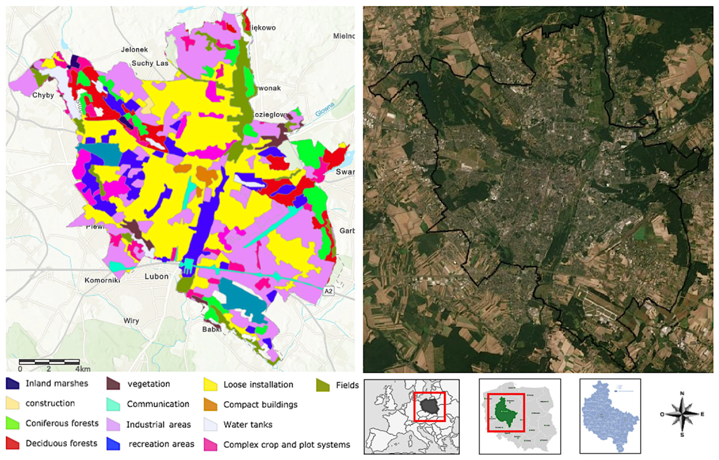
2.2. Study Area and Data

In former socialist countries, the transition from command- to market-oriented economies was followed by massive landownership transfers [21], leading to highly fragmented land use and a decrease in agriculture profitability with the consequent abandonment of the land. In this sense, Poland was not an exception.

In Poland, considerable FLA occurred during the period 1996–2002 and mainly concerned the grasslands. FLA appears to be located mainly in the east of the country, where there are small and diversified holdings, as opposed to the west, where during the communist period, many large holdings were state-owned farms [1]. With regard to urban areas and for this same period, the loss of UAA was estimated at 764,032 ha, corresponding to 36% of the total (urban and rural) decrease (30%, if we consider the net result). In municipalities with a density of over 200 inh/km², 35% of the UAA (633,193 ha) was lost during the period.

Specifically, Poznań was chosen as the case study area (Figure 3). According to the classification established by CORINE Land Cover, agricultural land covers 33% of the area of Poznań, and arable land clearly dominates (82%) the structure of this agricultural land. The main reason for choosing Poznań was because it has been greatly affected by landscape fragmentation and FLA over the past decade. As mentioned in Section 1, this abandonment has mainly been driven by permissive legislation or even by non-compliance with planning regulations. However, there has been another key factor in FLA: demographic evolution. Poznań has a specific demographic evolution, characterized by different flows occurring at the same time: (i) migration from some rural areas to urban areas, (ii) migration from city centers to peri-urban areas, and (iii) expansion of housing (catching up with the new lifestyle standards). Pushed by the development of the economy, these population flows create housing and infrastructure needs. The need for land is therefore becoming important in these urban areas.

Finally, and with regard to the data, we used high resolution aerial imagery provided by World_Imagery (MapServer) [22]. World_Imagery provides satellite and aerial imagery (with resolutions ranging from 0.5 m/pixel to 1 m/pixel) from many parts of the world. For further information on this data source, including the terms of use, visit online at [22]. In our case, the resolution of the image selected was 1 m/pixel.

2.3. Abandoned Farmland Extraction Algorithm

The main segmentation techniques based on observations of pixel tone analyze the shape of the greyscale histogram and classify the histogram clusters based on their sizes, splitting the original image. Although the resulting regions are visually different, they behave similarity with respect to certain statistical properties. However, this uniform statistical behavior is not usual in the majority of real imagery regions. Consequently, the use of pixel tone to segment imagery does not seem to be the best option [20]. To overcome this challenge, we developed an algorithm for extracting pixels from images based on a local-nonparametric approach to texture analysis. Textural segmentation can be defined as the process of partitioning an image into different parts together, which belong to the same object class. For this purpose, textural information is extracted from the image and used to develop tasks such as recognition, classification, and analysis [23]. In recent years, very discriminative and computationally efficient local texture descriptors have been developed [23]. Among all of these, our algorithm uses two main textural measures:

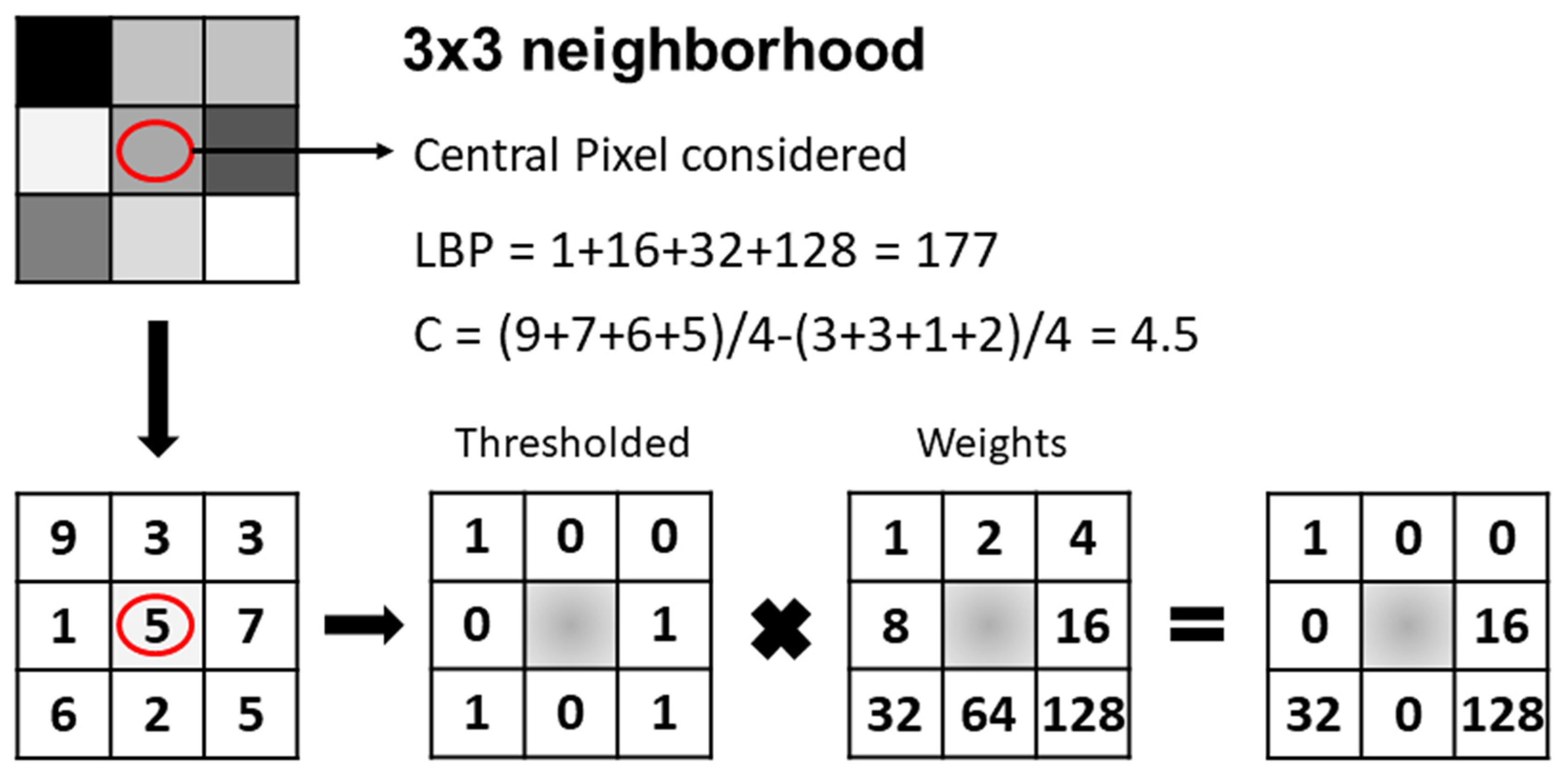
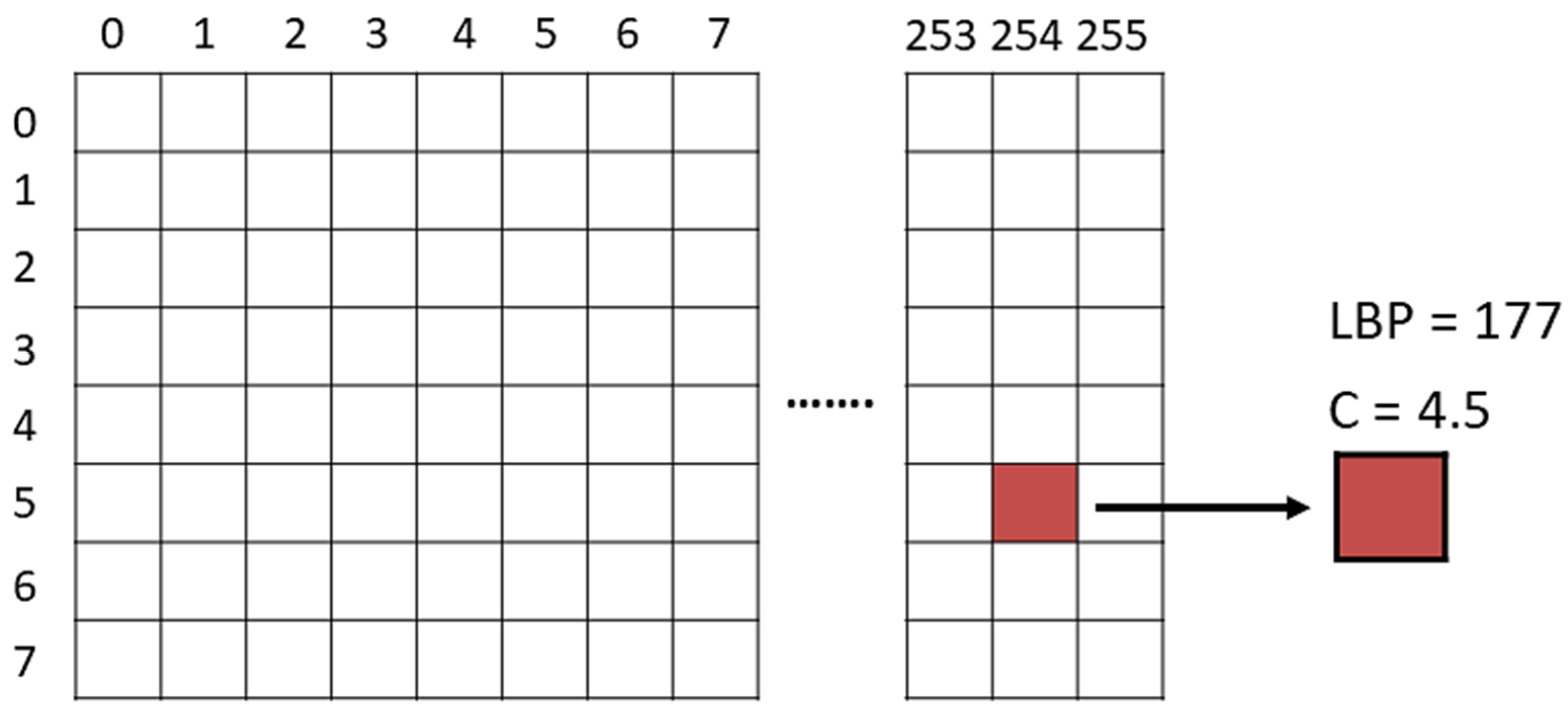
• Local binary pattern (LBP): LBP is a local texture descriptor capable of characterizing small texture regions [23]. LBP is a simple, yet very efficient texture operator that thresholds the neighboring pixels based on the value of the current pixel [24]. Due to its discriminative power, the LBP texture operator has become a popular approach in several applications, highlighting textural analysis procedures [25]. Figure 4 shows the procedure for computing LBP values. First, each central pixel is compared with its eight neighbors. This 3 × 3 neighborhood must be thresholded by the value of the center pixel; the neighbors having a smaller value than that of the central pixel will have bit 0, and the other neighbors having a value equal to or greater than that of the central pixel will have bit 1. Then these binary values of the pixels in the thresholded neighborhood must be multiplied by the weights given to the corresponding pixels. Finally, the values of the eight pixels will be added to obtain a number for this neighborhood. If we computed the LBP histogram over an entire region, it may be used for describing its texture. In addition, LBP achieves high levels of accuracy in textural characterization processes compared to other texture operators.
• A contrast measure (C): LBP descriptors efficiently capture the local spatial patterns. However, whereas LBP is invariant against any monotonic grey scale transformation, we must combine it with a simple contrast measure C to make it even more powerful. The computation of C is also addressed in Figure 4.

Six major steps define our FLA extraction procedure:

(1)

Texture characterization

As mentioned in the previous paragraphs, texture is not an image property that may be associated with a single pixel. That is why the image was decomposed into a grid where each of its cell included a fixed number of pixels. Its LBP/C distribution was approximated by a discrete two-dimensional histogram (array) of 256 × b pixels, where b is the number of bins for contrast measure C (Figure 5). This number of bins is chosen as a trade-off between the discriminative power and the stability of the texture description [17].

Once these histograms were obtained, the fundamental objective was to compare LBP/C distributions identifying two textures as equal or different. The tool that allowed us to make this identification was the G statistic [26]. Compared with other similarity statistic measures, such as log-cumulative distance or Jeffrey divergence [17,23], which present low discrimination capability, the G value (Equation (1)) is a non-parametric log-probabilistic statistic commonly used to assess the similarity between two histograms (A and B) when a high level of discrimination is required. Thus, the higher the value, the lower the similarity between them. In addition, in Equation (1), N represents the number of bins and fi represents the frequency at bin i.

$$G=2\left(\begin{array}{c}\hfill \left[{\displaystyle \sum _{A,B}}{\displaystyle \sum _{i=0}^N}{f}_{i}log{f}_i\right]-\left[{\displaystyle \sum _{A,B}}\right({\displaystyle \sum _{i=0}^N}{f}_i\left)log\right({\displaystyle \sum _{i=0}^N}{f}_i\left)\right]-\hfill \\ \hfill \left[{\displaystyle \sum _{i=0}^N}\right({\displaystyle \sum _{A,B}}{f}_i\left)log\right({\displaystyle \sum _{A,B}}{f}_i\left)\right]+\left[{\displaystyle \sum _{A,B}}{\displaystyle \sum _{i=0}^N}{f}_i\right)log\left({\displaystyle \sum _{A,B}}{\displaystyle \sum _{i=0}^N}{f}_i\right)]\hfill \end{array}\right)$$

(1)

(2)

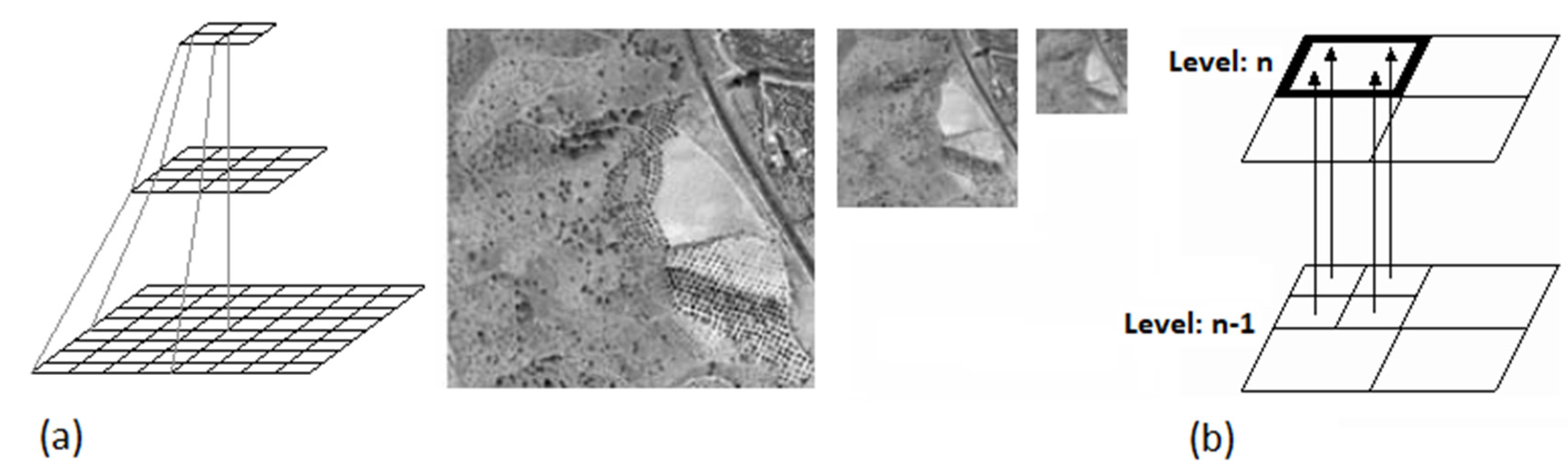
Hierarchical structure generation

With the main goal of optimizing the storage capacity and therefore improving the computation time, an approach based on a pyramidal representation was adapted to texture segmentation. Instead of performing image segmentation based on a single representation of the input image, a pyramid segmentation algorithm describes the contents of the image using multiple representations with decreasing resolution [27]. According to Marfil et al. [27], this type of algorithm exhibits interesting properties with respect to segmentation algorithms based on a single representation such as: (i) the detection of global features of interest and representing them at low resolution levels [28,29], (ii) the reduction of noise and the processing of local and global features within the same framework [30], and (iii) reduction in the complexity of the image segmentation task [28,29]. Specifically, we used a segmentation algorithm based on regular pyramids.

The general principle of our pyramidal approach was briefly described by Jolion and Montanvert [31]. According to that principle, a pyramidal architecture is completely defined if we specify how a new level is built (Figure 6a) and how a parent is linked to its children (Figure 6b). This parent-child relationship is defined by the reduction window and may be extended by transitivity down to the base level (Figure 6a). The set of children of one cell in the base level is named its receptive field [27], and it defines the embedding of this vertex in the original image. With regard to the efficiency of a pyramidal representation to solve a segmentation procedure, we must note that it is strongly influenced by the data structure used within the pyramid, limiting the information that may be encoded at each level, and the reduction scheme used, which defines its dynamics in terms of height and preservation of details [29].

In our pyramidal structure, a cell, at level l, represents a $2^l\times 2^l$ square in the input image, and the base of the structure is composed by the LBP/C distributions. Each pyramid cell, denoted by (x, y, l), has the following parameters associated with it:

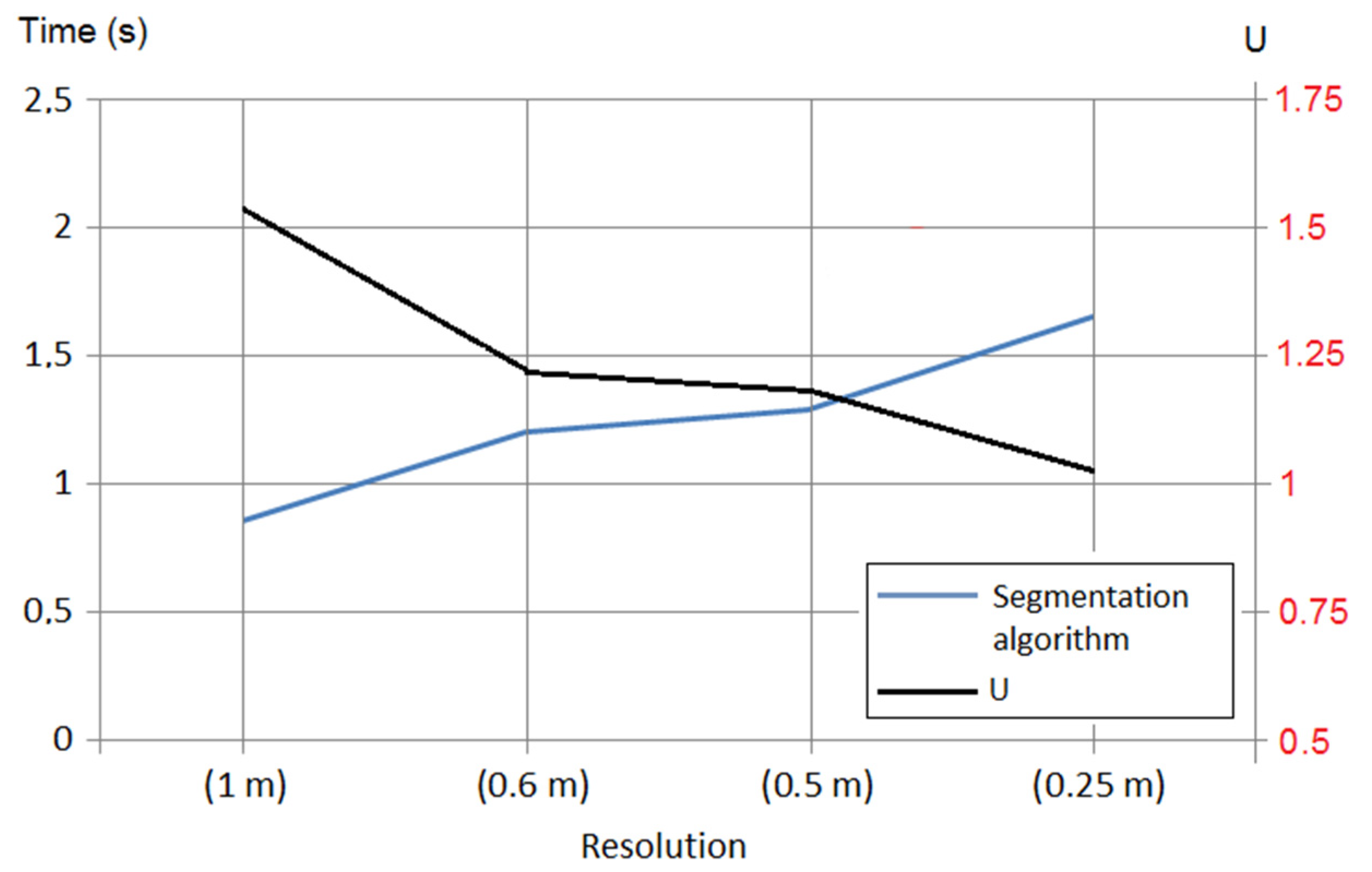
• Homogeneity, denoted by H(x, y, l). Homogeneity ranged from 1 (if the four cells immediately underneath had the same texture) to 0 (in any other case). The setting of H was based on a uniformity test. Thus, the four cells had the same texture if a measure of relative dissimilarity within that region was lower than a certain threshold U, ($G_{max}$/$G_{min}$ < U). U must be set in such a way as to ensure the detection and differentiation of textures, preventing wherever possible the inclusion of two regions with different textures in the same class. For this reason, it is advisable to choose a value for U as small as possible.
• Texture, denoted by T(x, y, l). The texture of one cell was calculated as the sum of the LBP/C distributions of the four cells immediately underneath if, and only if, the cell was homogeneous. Otherwise, the value of T(x, y, l) was set to a fixed value $(T_{NH})$.
• Parent link, denoted by ${\left(X,Y\right)}_{\left(x,y,l\right)}$. If $H_{\left(x,y,l\right)}$ was equal to 1, the values of the parent links of the four cells immediately underneath were set to (x, y). Otherwise, these four parent links were set to a null value.
• The centroid, denoted by $C_{\left(x,y,l\right)}$. $C_{\left(x,y,l\right)}$, represents the center of mass of the base region associated with (x, y, l).
• Histogram. Each parent link stored the two-dimensional histogram, which characterized the texture of the image region represented by this node. In order to optimize the storage capacity and to improve the computation time, if a node (located at the l level) represented a region of homogenous texture, all the nodes located at lower levels (until the end of the pyramid) did not store their corresponding histograms, their texture being characterized by the histogram stored in the parent link.

After completing the hieratical structure generation (Step Number 2), all the cells belonging to this structure with a homogeneity value equal to 1 and having no parent were linked to homogeneous regions at the base, defining initial image segmentation.

(3)

Grow of homogeneous cells

In this step, the algorithm linked cells whose parent link values were null. Basically, a cell (x, y, l) was linked to the parent of its neighbors (xp, yp, l+1) when two cells had the same texture.

(4)

Homogeneous cells fusion

The neighbor cells, (x1, y1, l) and (x2, y2, l), were merged if the following four conditions were true:

• ${\left(X,Y\right)}_{\left(x1,y1,l\right)}$ = null. Therefore, the cell had no parent.
• ${\left(X,Y\right)}_{\left(x2,y2,l\right)}$ = null. Therefore, the cell had no parent.
• The cells had a homogeneous texture. $H_{\left(x1,y1,l\right)}$ = 1 & $H_{\left(x2,y2,l\right)}$ = 1.
• The cells had the same texture.

(5)

Pixel-wise

Since pixels at the base level of the pyramid were treated as blocks, the resolution of the segmented image R was represented by Equation (2), where S is the resolution of the initial image and A is the area of the pixels averaged to create a cell.

$$R=S/A$$

(2)

In order to improve the resolution of the output image and therefore to decrease the segmentation error, a post-processing step was developed. This post-processing was based on a type of segmentation procedure called soft segmentation [32], in which each pixel can belong to more than one region, thereby avoiding mistakes in region boundaries. When an image is segmented, pixels near region boundaries are usually intermediate in value between the regions, and they can be placed in either of them during the cell fusion [27]. Considering this, first, our algorithm recursively increased the resolution of all blocks in texture region boundaries until those boundaries were a pixel wide and then built the segmentation probability map. This probability map indicated the probability of each pixel that belonged to one of the predefined classes, and it was built on the basis of the texture parameter ${\left(LBP,C\right)}_{FLA}$ values learned from the training procedure explained in the next paragraph. From these data, several closed segmentation contours were generated, and the final textural segmentation was obtained.

(6)

FLA zones’ extraction

After resolving the segmentation issue, we had to identify and separate FLA zones from the rest. We had an image that contained multiple zones such as vegetation, constructions, etc. In this phase, we extracted and rebuilt the FLA zones from the image. In order to extract the FLA zones, we needed to remove the objects that did not possess the textural properties of FLA. Without losing generality, our main assumption about FLA on images was: unlike other vegetation zones or construction zones, which could have many different texture models, FLA zones usually had the same kind of texture model due to the representative properties of the terrain and vegetation that characterized them. Based on this assumption, we trained the system on different areas of the image to learn the FLA zones’ texture parameters ${\left(LBP,C\right)}_{FLA}$; thereby generating a set of thresholds for these texture parameters. In this regard, it is very important to recall that although LBP achieves high levels of accuracy in textural characterization processes compared with other texture operators, these thresholds (linked to the training procedure) generate uncertainty during the classification process. In addition, and in order to increase as much as possible the robustness of the results, these training areas should not include the cadastral plots employed for evaluating the segmentation results (test plots) (described in the next subsection).

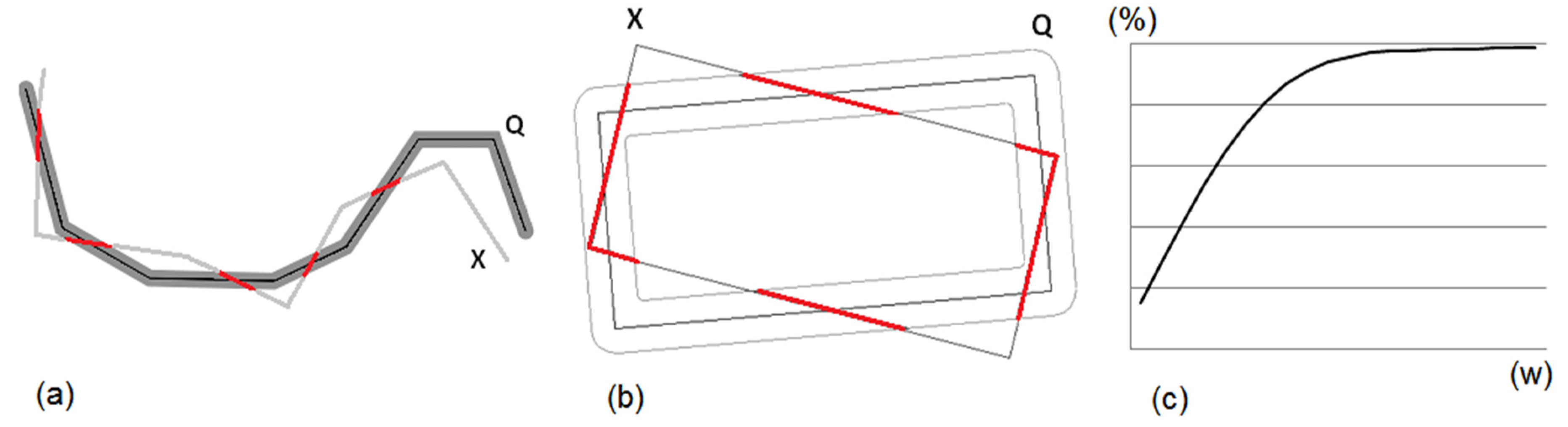
2.4. Evaluation of Segmentation Results

As several authors and studies have pointed out [17,18,23], it is not easy to assure that an algorithm provides a final “good” segmentation of the image. In general, “it is not clear what a ‘good’ segmentation is” [29], and it is necessary to have the opinion of a human expert who decides the final accuracy of the studied algorithm. Therefore, the measure of the segmentation quality depends on human intuition and could be different for distinct observers. In order to overcome this inconvenience, we developed a methodology that sought to avoid distortions and biases caused by human intervention in the process.

According to the classification established by Marfil et al. [27], our method could be classified as a discrepancy method. Discrepancy methods are quantitative and empirical procedures that use the ideal segmentation (reference data) for assessing the quality of the segmentation obtained with an algorithm (tested or assessed data) by counting the differences between both datasets. If these differences are expressed in terms of spatial position or location, then discrepancy methods have the same conceptual framework as the automatic procedure employed for assessing the positional accuracy of geospatial databases (using linear elements) developed by Ruiz-Lendínez et al. [33]. Specifically, these authors used the single buffer overlay method (SBOM) (Figure 7). Based on buffer generation on the line of the source of greater accuracy (Q) (reference data), this method determines the percentage of the controlled line (X) (tested or assessed data) that is within this buffer (Figure 7a). By increasing the width of the buffer, a probability distribution of inclusion of the controlled line inside the buffer of the source of greater accuracy is obtained (Figure 7c). Finally, Figure 7b shows the adaptation of this metric to the line-closed case carried out by Ruiz-Lendínez et al. [33].

In view of the above, discrepancy methods do not depend on human intuition, but in compensation, they present the problem that having a previous ideal segmentation is necessary. In many fields, research based on pattern recognition might be a problem. However, in the case of geographical data, finding a source of greater accuracy (reference data) is relatively simple. In our specific case, the ideal segmentation (reference data) is represented by a sample of cadastral plots (test plots) whose geometry is known (a priori) with high accuracy, and as test data, we used these same plots obtained by applying our abandoned farmland extraction algorithm. In this second case (test data), the boundaries of the test plots were obtained by means of a vectorization procedure.

Finally, in order to implement our methodology, we employed all the parcels present in the control sample, obtaining an aggregated distribution curve. The number and characteristics of this set of plots is specified in the next subsection.

2.5. Evaluation of the Efficiency of Our Approach for Locating Abandoned Land

As mentioned in the Introduction section, the effectiveness of the proposed methodology was assessed not only from a segmentation results perspective, but also taking into account the efficiency of our approach for locating the abandoned land. In this second case, the accuracy in training the algorithm to learn the FLA zone texture parameters ${\left(LBP,C\right)}_{FLA}$ was key to achieving an accurate land use classification, with LBP values able to appear out of the range characteristic of FLA zones, increasing uncertainty during the classification process. For this reason, and in order to check the land use, two inspection procedures were carried out: (i) an external validation based on a visual inspection procedure through field visits and (ii) a revision of the LBP/C parameters belonging to the sample of test plots. Since we had two different observations from two different inspection procedures, we applied Cohen’s Kappa coefficient [34] in order to determine the land use. Cohen’s Kappa coefficient (k) (Equation (3)) measures the concordance between two different observations in their corresponding classifications of N elements in C mutually exclusive categories. K is a more robust measure than the simple calculation of the percentage of concordance, since it takes into account the agreement that occurs by chance.

$$k=\frac{P_r\left(a\right)-P_r\left(e\right)}{1-P_r\left(e\right)}$$

(3)

where $P_r\left(a\right)$ is the relative observed agreement between both observations and $P_r\left(e\right)$ is the hypothetical probability of agreement by chance using the observed data to calculate the probabilities of each observer (inspection procedure) randomly classifying each category. With regard to the k value interpretation: (i) if both observations fully agree, then k = 1, and (ii) if there is no agreement between the observations other than what would be expected by chance (as defined by $P_r\left(e\right)$), then k = 0 [34].

Finally, and with regard to the number and characteristics of the test plots, we selected 40 plots uniformly distributed over the study area. Therefore, N = 40 elements (sample of plots), and C = 2 categories (land classified as abandoned or land classified as other use). Obviously, in order to increase as much as possible the robustness of the results and avoid possible biases, these plots did not overlap with training areas employed for learning the FLA texture parameters.

3. Results

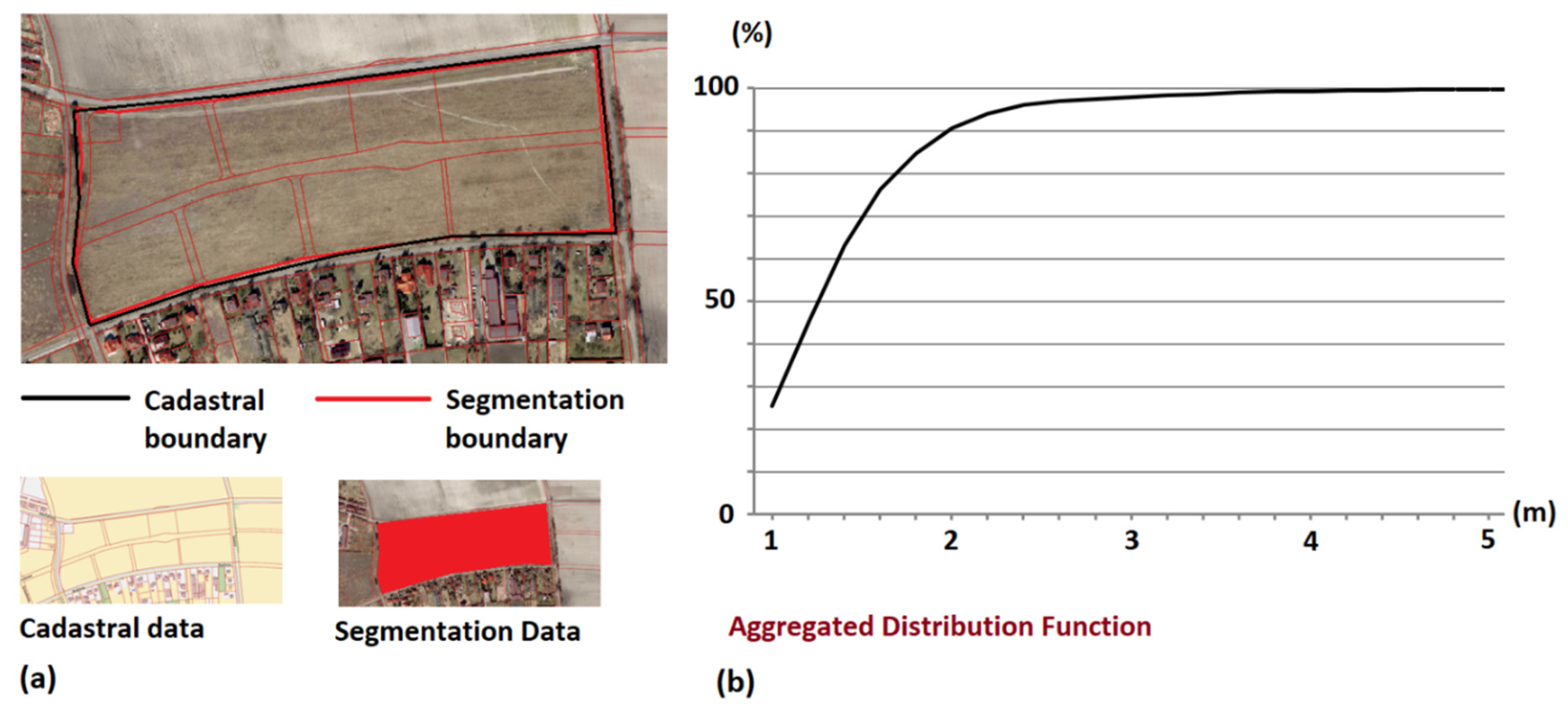
3.1. Mapping Abandoned Farmland Derived From Textural Segmentation of the Aerial Image

Based on a visual interpretation of the derived map, the model was able to capture the pattern of abandoned land in the areas affected by rapid urbanization. Figure 8 shows that: (i) abandoned arable land was located mainly in the northern and western parts of the city, which corresponded to the main direction of the urbanization process of Poznań; (ii) by comparing the results obtained with the data provided by CORINE Land Cover, 2275 ha (40.3%) of arable land within the city limits were abandoned; and (iii) the area of abandoned arable land was almost 9.2% of the city’s area.

3.2. Evaluation of Segmentation Results

As mentioned in Section 2.3, we used SBOM (specifically, an adaptation of its metric to the line-closed case) to assess the quality of the segmentation obtained with our algorithm (Figure 9a). Figure 9b presents the resulting aggregated distribution function by applying SBOM on our two datasets, that is to say, plot boundary lines from the cadastral data and plot boundary lines from the results provided by our abandoned farmland extraction algorithm (segmentation boundaries) using buffers with widths from 1 to 5 m. It is important to note that in this second case, the boundaries of these test plots were obtained by means of a vectorization procedure.

The aggregated curve obtained with our method showed a distribution function of the uncertainty for several levels of confidence. Figure 9b shows a value around 2.4 m for a 95% level of confidence. Taking into account the resolution of the image and the uncertainty associated with the vectorization procedure, this value seemed to be a priori acceptable.

In any case, and in order to check the goodness of this measure, it was tested by means of the empirical evaluation method proposed by Liu and Yang [35], which was based on calculating the differences between the original image and the segmented image using the area of the segmented regions as a reference parameter. In accordance with this and taking into account the mean value of the test plot area, a variation in the width of the buffer of 2.4 m (±1.2 m) on the perimeter of the plots represented less than 0.35% of the segmentation surface.

3.3. Evaluation of the Efficiency of Our Approach for Locating Abandoned Land

As mentioned in Section 2.4, in order to determine the land use obtained from our derived map (Figure 8), we applied Cohen’s Kappa coefficient in two different inspection procedures: (i) a visual inspection procedure through field visits and (ii) a revision of the LBP/C parameters belonging to the sample of test plots.

Table 1. Results of the analysis of each inspection procedure.

		Field visit
		Abandoned Land	Other Uses
Revision of LBP/C parameters	Abandoned Land	36	2
	Other uses	1	1

shows the results of the analysis of each inspection procedure.

The values located on the first diagonal (36,1) represent the total number of plots in which there was agreement between both inspection procedures. The second diagonal, composed of the values of one and two, represent those plots in which there was disagreement between them. Taking into account these results, the percentage of agreement was 92.5%. In order to calculate the probability that the agreement between both inspection procedures was due to chance, we must take into account that:

• The number of plots classified as abandoned land by means of the field visit procedure was 37, and the number of plots classified as “other uses” was three. Consequently, by means of this procedure, 92.5% of plots were classified as abandoned land.
• The number of plots classified as abandoned land by means of revision of the LBP/C parameters was 38, and the number of plots classified as “other uses” was two. Consequently, by means of this procedure, 95% of plots were classified as abandoned land.

Therefore, the probability that both procedures classified the plots as abandoned land at random was 87.8%, while the probability that both procedures classified the plots as “other uses” at random was 0.37%. From this, we deduced that the probability that the agreement between both inspection procedures was due to random was 88.2%. Finally, applying Equation (3), we obtained a K value equal to 0.82. This value represented a high level of concordance between both observations (inspection procedures).

4. Discussion

This paper presented a quick and easy method for mapping abandoned land in cities affected by rapid urbanization by using textural characterization of high resolution aerial imagery. Our method, which employed free data provided by World_Imagery (MapServer) [22], was relevant because: (i) it produced land use maps under conditions in which time and human resources were scarce; and (ii) it had significant socioeconomic impact.

Concerning the first aspect (time), our approach was particularly efficient in comparison with other alternatives such as SRS. Mapping abandoned land using high resolution aerial imagery did not require the pre-processing phases or classification procedures inherent to satellite platforms. Such procedures were replaced by a training phase on different areas of the image to learn the FLA zones’ texture parameters ${\left(LBP,C\right)}_{FLA}$, significantly reducing the computational time necessary to obtain the final map. With regard to the computation process itself, the computational efficiency of our algorithm depended on (i) the threshold U (see the section “Hierarchical Structure Generation”) and (ii) the number of textural regions in the image. To achieve the segmentation of higher resolution images, the algorithm required more computation time because in this case, a value for U as small as possible was required.

As mentioned in the Introduction section, our approach to texture characterization was already successfully tested in other studies [19,20]. Although both their purpose and the features used differed from those addressed here, these studies were very useful when the relationship between computation time, image resolution, and threshold “U” was analyzed because the results obtained could be extrapolated to other types of segmentation processes. In our case, this was particularly useful for setting U.

Figure 10 shows the relationship obtained for the parameters mentioned above: time, U, and resolution. According to the values shown in Figure 10 and taking into account the resolution of our image (1 m), the value for the threshold U was set to 1.5. Finally, the computation time obtained for our case of study was 15.3 s. This value was higher than expected. This was due to: (i) the large size of our study area and (ii) the need to process the entire image because in our case, it was not possible to apply localized spatial filters, such as localized template matching (LTM) [36]. In this respect, we must start pointing out that our test platform was an Intel Core i5 3.8 GHz with 16 GB of memory.

Concerning socioeconomic impact, locating trends and patterns of FLA could help authorities in developing urban policies, providing objective information to municipalities where official statistics on land abandonment are unreliable or of low quality. Our approach could be used by local authorities that cannot allocate significant resources for land change monitoring. In addition, it provided a useful tool for spatial management, as well as for cadastral tax purposes and could be applied to any city, metropolitan area, or spatial region.

5. Conclusions

This study helped to understand how the textural characterization of high resolution aerial imagery could be used for locating and mapping FLA. We employed a textural segmentation algorithm that had already been successfully tested in other types of processes based on the automatic extraction of geographical entities from imagery. As in those processes, our algorithm proved to be an effective and valuable tool for locating and extracting abandoned farmland from imagery in areas affected by rapid urbanization. Among all local texture descriptors, we employed texture descriptors based on LBP combined with a simple contrast measure to make our method more powerful. LBP provided us with knowledge about the spatial structure of the local image texture and was very efficient from a computational point of view. In addition, LBP achieved high levels of accuracy in textural characterization processes compared with other texture operators. With regard to the structure, our algorithm was implemented on a pyramidal representation, which significantly reduced computation time and assured robustness.

The effectiveness of the proposed methodology was assessed from two different perspectives: (i) the accuracy of the segmentation results and (ii) the efficiency for locating FLA. In the first case, we developed an innovative methodology based on the procedures employed for assessing the positional accuracy of geospatial databases. This methodology provided us an uncertainty value (of the segmented plots) of around 2.4 m with regard to the source of greater accuracy employed (cadastral data). In the second case, we employed two different empirical inspection procedures, measuring (and confirming) the concordance between them.

With regard to the results, the model obtained allowed us to identify the patterns of abandoned land in the city. These patterns corresponded to the main direction of the urbanization process of Poznań, that is to say to those areas affected by rapid urbanization in the city. The area of abandoned arable land was almost 9.2% of the city’s area. Finally, comparing the results obtained with the data provided by CORINE Land Cover, 2275 ha (40.3%) of arable land within the city limits were abandoned.

Finally, we must note that our study could support local authorities in adapting urban planning for a more efficient use of land.

Finally, this study represents only a further step towards the improvement in the location and management of abandoned land. Thus, although our algorithm solved the problem in an effective way, the inspection procedures carried out revealed some inconsistences during the process of classification, possibly derived from the training phase (developed to learn the FLA zones’ texture parameters ${\left(LBP,C\right)}_{FLA}$). In this sense, the use of artificial intelligence mechanisms could help to classify FLA zones much more efficiently. This would imply the inclusion in the process of other texture descriptors that would increase the levels of discrimination. On the other hand, although our approach identified FLA zones, it was unable to determine the quality of the soil they occupied, which made it impossible to assess the real scope of the problem.

All these challenges must be addressed in future works. Thus, we plan the incorporation of genetic algorithms (GA) in the learning process mentioned above, adding new (and more powerful) texture descriptors. In this respect, some previous studies [37] already demonstrated that GA was an appropriate and efficient learning method for problems where spatial variables were implied. With regard to the quality of the soil occupied by FLA zones, we plan to compare our map of abandoned land with maps of soil quality provided by local and regional authorities. This will allow us to verify if a significant part of arable land that is of the biggest importance for agriculture is still being cultivated in the city or, conversely, that these soils should be urgently protected.

References

1. Pointereau, P.; Coulon, F.; Girard, P.; Lambotte, M.; Stuczynski, T.; Sanchez-Ortega, V.; Del Rio, A. Analysis of Farmland Abandonment and the Extent and Location of Agricultural Areas that are Actually Abandoned or are in Risk to be Abandoned; Anguiano, E., Bamps, C., Terres, J., Eds.; Institute for Environment and Sustainability, Joint Research Centre, European Commission: Luxembourg, 2008. [Google Scholar]
2. Grădinaru, S.; Kienast, F.; Psomas, A. Using multi-seasonal Landsat imagery for rapid identification of abandoned land in areas affected by urban sprawl. Ecol. Indic. 2019, 96, 79–86. [Google Scholar] [CrossRef]
3. Benayas, J.; Martins, A.; Nicolau, J.; Schulz, J. Abandonment of agricultural land: An overview of drivers and consequences. CAB Rev. Perspect. Agric. Vet. Sci. Nutr. Nat. Resour. 2007, 2, 1–14. [Google Scholar] [CrossRef] [Green Version]
4. Morán, N.; Hernández, V.; Zazo, A.; Simón, M. Multifuncionalidad, preservación y retos futuros de la agricultura peri-urbana en la Europa mediterránea. In Agricultura Urbana Integral, Ornamental y Alimentaria; Briz, J., De Felipe, I., Eds.; Ministerio de Agricultura, Alimentación y Medio Ambiente Press: Madrid, Spain, 2015; pp. 153–170. [Google Scholar] [CrossRef] [Green Version]
5. Wulder, M.; Hall, R.; Coops, N.; Franklin, S. High spatial resolution remotely sensed data for ecosystem characterization. Bioscience 2004, 54, 511–521. [Google Scholar] [CrossRef] [Green Version]
6. Huzui, A.; Abdelkader, A.; Pătru -Stupariu, I. Analysing urban dynamics using multi-temporal satellite images in the case of a mountain area, Sinaia (Romania). Int. J. Digit. Earth 2011, 6, 1–17. [Google Scholar]
7. Kolecka, N.; Kozak, J.; Kaim, D.; Dobosz, M.; Ginzler, C.; Psomas, A. Mapping secondary forest succession on abandoned agricultural land with LiDAR point clouds and terrestrial photography. Remote Sens. 2015, 7, 8300–8322. [Google Scholar] [CrossRef] [Green Version]
8. Grădinaru, S.; Lojă, C.; Onose, D.; Gavrilidis, A.; Pătru-Stupariu, I.; Kienast, F.; Hersperger, A. Land abandonment as precursor of built-up development at the sprawling periphery of former socialist cities. Ecol. Indic. 2015, 57, 305–313. [Google Scholar] [CrossRef]
9. Estel, S.; Kuemmerle, T.; Alcántara, C.; Levers, C.; Prishchepov, A.; Hostert, P. Mapping farmland abandonment and recultivation across Europe using MODIS NDVI time series. Remote Sens. Environ. 2015, 163, 312–325. [Google Scholar] [CrossRef]
10. Liu, N.; Harper, R.; Handcock, R.; Evans, B.; Sochacki, S.; Dell, B.; Walden, L.; Liu, S. Seasonal Timing for Estimating Carbon Mitigation in Revegetation of Abandoned Agricultural Land with High Spatial Resolution Remote Sensing. Remote Sens. 2017, 9, 545. [Google Scholar] [CrossRef] [Green Version]
11. Stryjakiewicz, T.; Królewicz, S.; Ruiz-Lendinez, J.J.; Mickiewicz, B.; Motek, P. Abandoned agricultural land quantification in urban areas using high resolution satellite imagery. In Proceedings of the RSA Central and Eastern Europe Conference: Metropolises and Peripheries of CEE Countries: New Challenges for EU, National and Regional Policies, Lublin, Poland, 11–13 September 2019. [Google Scholar]
12. Baumann, M.; Kuemmerle, T.; Elbakidze, M.; Ozdogan, M.; Radeloff, V.C.; Keuler, N.S.; Prishchepov, A.V.; Kruhlov, I.; Hostert, P. Patterns and drivers of post-socialist farmland abandonment in Western Ukraine. Land Use Policy 2011, 28, 552–562. [Google Scholar] [CrossRef]
13. Prishchepov, A.; Radeloff, V.; Baumann, M.; Kuemmerle, T.; Muller, D. Effects of institutional changes on land use: Agricultural land abandonment during the transition from state-command to market-driven economies in post-Soviet Eastern Europe. Environ. Res. Lett. 2012, 7, 024021. [Google Scholar] [CrossRef]
14. Prishchepov, A.; Radeloff, V.; Dubinin, M.; Alcantara, C. The effect of Landsat ETM/ETM + image acquisition dates on the detection of agricultural land abandonment in Eastern Europe. Remote Sens. Environ. 2012, 126, 195–209. [Google Scholar] [CrossRef]
15. Bazzi, H.; Baghdadi, N.; El Hajj, M.; Zribi, M.; Minh, D.H.T.; Ndikumana, E.; Courault, D.; Belhouchette, H. Mapping Paddy Rice Using Sentinel-1 SAR Time Series in Camargue, France. Remote Sens. 2019, 11, 887. [Google Scholar] [CrossRef] [Green Version]
16. Carrasco, L.; O’Neil, A.; Morton, R.; Rowland, C. Evaluating Combinations of Temporally Aggregated Sentinel-1, Sentinel-2 and Landsat 8 for Land Cover Mapping with Google Earth Engine. Remote Sens. 2019, 11, 288. [Google Scholar] [CrossRef] [Green Version]
17. Ojala, T.; Pietikäinen, M. Unsupervised texture segmentation using feature distributions. Pattern Recognit. 1999, 32, 477–486. [Google Scholar] [CrossRef] [Green Version]
18. Maenpaa, T.; Pietikäinen, M. Texture analysis with local binary patterns. In Handbook of Pattern Recognition and Computer Vision; Chen, C., Wang, P., Eds.; University of Massachusetts Dartmouth Press: Dartmouth, MA, USA, 2005; pp. 197–216. [Google Scholar] [CrossRef]
19. Ruiz-Lendínez, J.J.; Rubio-Campos, T.J.; Ureña-Cámara, M.A. Automatic extraction of road intersections from images based on texture characterization. Surv. Rev. 2011, 43, 212–225. [Google Scholar] [CrossRef]
20. Ruiz-Lendínez, J.J.; Maćkiewicz, B.; Motek, P.; Stryjakiewicz, T. Method for an automatic alignment of imagery and vector data applied to cadastral information in Poland. Surv. Rev. 2019, 51, 123–134. [Google Scholar] [CrossRef]
21. Kuemmerle, T.; Muller, D.; Griffiths, P.; Rusu, M. Land use change in Southern Romania after the collapse of socialism. Reg. Environ. Change 2009, 9, 1–12. [Google Scholar] [CrossRef]
22. World Imagery. Available online: http://goto.arcgisonline.com/maps/World_Imagery (accessed on 10 February 2020).
23. Pietikäinen, M.; Zhao, G. Two decades of local binary patterns: A survey. In Advances in Independent Component Analysis and Learning Machines; Academic Press: Oxford, UK, 2015; pp. 175–210. [Google Scholar]
24. Malhotra, A.; Sankaran, A.; Mittal, A.; Vatsa, M.; Singh, R. Fingerphoto Authentication Using Smartphone Camera Captured Under Varying Environmental Conditions. In Using Computer Vision, Pattern Recognition and Machine Learning Methods for Biometrics; Academic Press: Oxford, UK, 2017; pp. 119–144. [Google Scholar]
25. Dornaika, F.; Moujahid, A.; El Merabet, Y.; Ruichek, Y. A Comparative Study of Image Segmentation Algorithms and Descriptors for Building Detection. In Handbook of Neural Computation; Academic Press: Oxford, UK, 2017; pp. 591–606. [Google Scholar]
26. Sokal, R.; Rohlf, F. Introduction to Biostatistics; W.H. Freeman & Co. Ltd: Gordonsville, Virginia, USA, 1987. [Google Scholar]
27. Marfil, R.; Molina-Tanco, L.; Bandera, A.; Rodríguez, J.; Sandoval, F. Pyramid segmentation algorithms revisited. Pattern Recognit. 2006, 39, 1430–1451. [Google Scholar] [CrossRef] [Green Version]
28. Cho, K.; Meer, P. Image segmentation from consensus information. Comput. Vis. Image Underst. 1997, 68, 72–89. [Google Scholar] [CrossRef] [Green Version]
29. Kropatsch, W.; Haxhimusa, Y. Grouping and segmentation in a hierarchy of graphs. In Computational Imaging II; SPIE Press; Digital Library: Bellingham, WA, USA, 2004; pp. 193–204. [Google Scholar]
30. Bister, M.; Cornelis, J.; Rosenfeld, A. A critical view of pyramid segmentation algorithms. Pattern Recognit. Lett. 1990, 11, 605–617. [Google Scholar] [CrossRef]
31. Jolion, J.M.; Montanvert, A. The adaptive pyramid, a framework for 2D image analysis. Comput. Vis. Image Underst. 1992, 55, 339–348. [Google Scholar] [CrossRef]
32. Prewer, D.; Kitchen, L.J. Soft image segmentation by weighted linked pyramid. Pattern Recognit. Lett. 2001, 22, 123–132. [Google Scholar] [CrossRef]
33. Ruiz-Lendínez, J.J.; Ariza-López, F.J.; Ureña-Cámara, M.A. Automatic positional accuracy assessment of geospatial databases using line-based methods. Surv. Rev. 2013, 45, 332–342. [Google Scholar] [CrossRef]
34. Cohen, J. A coefficient of agreement for nominal scales. Educ. Psychol. Meas. 1960, 20, 37–46. [Google Scholar] [CrossRef]
35. Liu, J.; Yang, Y. Multi-resolution color image segmentation. IEEE Trans. Pattern Anal. Mach. Intell. 1994, 16, 689–700. [Google Scholar]
36. Chen, C.; Knoblock, C.; Shahabi, C. Automatically conflating road vector data with orthoimagery. Geoinformatica 2006, 10, 495–530. [Google Scholar] [CrossRef] [Green Version]
37. Ruiz-Lendínez, J.J.; Ariza-López, F.J.; Ureña-Cámara, M.A. A polygon and point-based approach to matching geospatial features. ISPRS Int. J. Geo-Inf. 2017, 6, 399. [Google Scholar] [CrossRef] [Green Version]
Figure 1. The frontier between utilized agricultural land, non-utilized agricultural land, and forest.
Ijgi 09 00191 g001
Figure 2. Workflow of the proposed methodology.
Ijgi 09 00191 g002
Figure 3. Location of the study area (Poznań), classification established by CORINE Land Cover and the high resolution aerial image selected. Source: https://www.arcgis.com/apps/webappviewer.
Ijgi 09 00191 g003
Figure 4. Computation of local binary patterns (LBP) and the contrast measure (C).
Ijgi 09 00191 g004
Figure 5. Bidimensional array of LBP/C.
Ijgi 09 00191 g005
Figure 6. Hierarchical structure. (a) Set of pyramidal structures from texture; (b) parent link.
Ijgi 09 00191 g006
Figure 7. (a) Buffer generation by means of single buffer overlay method (SBOM). (b) Adaptation to the line-closed case (polygons or plots). (c) Empirical probabilistic distribution function.
Ijgi 09 00191 g007
Figure 8. Map of abandoned land as derived from textural segmentation of the aerial image.
Ijgi 09 00191 g008
Figure 9. (a) Single buffer overlay method (SBOM) adapted to the line-closed case: the cadastral boundary represents the line of the source of greater accuracy (Q), and the segmentation boundary represents the controlled line (X); (b) aggregated distribution function.
Ijgi 09 00191 g009
Figure 10. Computation time vs. image resolution and U.
Ijgi 09 00191 g010