General Method for Extending Discrete Global Grid Systems to Three Dimensions


Department of Computer Science, University of Calgary, Calgary, AB T2N 1N4, Canada
*
Author to whom correspondence should be addressed.
ISPRS Int. J. Geo-Inf. 2020, 9(4), 233; https://0-doi-org.brum.beds.ac.uk/10.3390/ijgi9040233
Submission received: 24 February 2020
/
Revised: 20 March 2020
/
Accepted: 8 April 2020
/
Published: 10 April 2020
(This article belongs to the Special Issue Global Grid Systems)
Abstract
:Geospatial sensors are generating increasing amounts of three-dimensional (3D) data. While Discrete Global Grid Systems (DGGS) are a useful tool for integrating geospatial data, they provide no native support for 3D data. Several different 3D global grids have been proposed; however, these approaches are not consistent with state-of-the-art DGGSs. In this paper, we propose a general method that can extend any DGGS to the third dimension to operate as a 3D DGGS. This extension is done carefully to ensure any valid DGGS can be supported, including all refinement factors and non-congruent refinement. We define encoding, decoding, and indexing operations in a way that splits responsibility between the surface DGGS and the 3D component, which allows for easy transference of data between the 2D and 3D versions of a DGGS. As a part of this, we use radial mapping functions that serve a similar purpose as polyhedral projection in a conventional DGGS. We validate our method by creating three different 3D DGGSs tailored for three specific use cases. These use cases demonstrate our ability to quickly generate 3D global grids while achieving desired properties such as support for large ranges of altitudes, volume preservation between cells, and custom cell aspect ratio.
1. Introduction
The near-ubiquity of certain smart technologies (smartphones, LIDAR, autonomous vehicles, UAVs, drones) is leading to an increasing amount of spatial information and data being generated [1]. Because of this, the development of technologies and tools for managing these types of data, along with other conventional geographic information, is more important than ever. Geographic information systems (GIS) have traditionally been used for this task, where different datasets are represented as individual layers in a two-dimensional (2D)—or if altitude is represented a three-dimensional (3D)—coordinate system, which acts as a proxy for the Earth [2,3]. However, the distortion and map edges that result from projecting the surface of the Earth to a plane can affect the accuracy of certain analyses [4,5] and also result in misleading visualizations if one is not careful [6]. Furthermore, when a large volume of data is present, overlaying operations such as intersection and data extraction become computationally expensive [7].
An alternative to the coordinate-based approach of GIS for managing geospatial data is an area, or cell, based system. A partitioning of the Earth into a set of non-overlapping cells allows information to be associated with the cell(s) that correspond with the appropriate region(s) of the Earth. Such partitionings are termed discrete global grids. To accommodate different resolutions of data, a hierarchy of these discrete global grids at successively finer resolutions, referred to as a discrete global grid system (DGGS), can be used [8]. Current state-of-the-art DGGSs make use of an approximating polyhedron as an initial discretization of the Earth’s surface [9,10,11], and are the class of DGGS this work will focus on.
Many of the geospatial sensors mentioned above, along with other technologies such as numerical weather prediction, generate 3D geospatial data, that is, data with an associated altitude in addition to the surface coordinates. While DGGSs are effective for integrating and managing geospatial data on the surface of the Earth, they have no inbuilt mechanisms for supporting 3D data. Because of this, there has been a recent push toward developing technologies for 3D global grids and grid systems [12]. While most 3D geospatial data are located in a relatively small region above and below the surface of the Earth, vital processes such as seismic wave propagation and the magnetosphere extend much beyond this narrow region. Additionally, satellites in high Earth orbit have altitudes exceeding 35,000 km. Therefore, in order to support the full range of human activity and interest, there may be a need for 3D global grids to extend far beyond the atmosphere and toward the centre of the Earth.
Approaches for creating 3D global grid systems exist [13,14,15], however current methods are typically based on latitude-longitude coordinates and are not consistent with current state-of-the-art DGGSs. Ideally, a new 3D global grid system should leverage the research, development, and data collection achieved with conventional DGGS. One way to create such a grid is by extending an existing DGGS to the third dimension to operate as a 3D global grid system. However, there are many different DGGSs with various desirable properties [16,17,18,19], and as such, the ideal DGGS to be extended depends on the application. Instead of extending a single DGGS to 3D, a more versatile approach is to create a general method that works for any arbitrary DGGS. This extension should be done in such a way that the resulting 3D grid is fully compatible with the conventional (2D) one, meaning that it allows efficient and straightforward transference of data between the two grids, both from 2D to 3D and from 3D to 2D. The 3D grids should also preserve—as best as possible—desirable properties of the conventional DGGS such as area, or in 3D volume, preservation.
In this paper, we introduce a general method for creating 3D global grid systems that use a conventional DGGS—which we refer to as the input DGGS—as a starting point and specification. We call the resulting grid system a 3D DGGS. These 3D DGGSs provide a natural extension of the input DGGS to the third dimension and are fully compatible with their respective surface representations. An overview of the method for creating the geometry of the grid is detailed in Figure 1. For constructing the base cells, we simply extend the faces of the input DGGS polyhedron to the desired vertical extent, resulting in prismatoid shaped cells. A refinement method is then needed to create more fine resolutions of the grid from these cells. For base cells with a large radial extent, regular 3D refinement introduces significant variation in cell shape and size. This degeneration is a natural consequence of the prismatoid cells converging at the centre of the grid. To address this issue, we construct a semiregular refinement method that achieves improved cell uniformity. Both the regular and semiregular refinements are based on the refinement used in the input DGGS. Our method works for all valid DGGS refinements, including all refinement factors and non-congruent schemes. We also provide refinement rules to control the aspect ratio (width compared to depth) of cells in the grid.
With the geometry of the grid defined, a method for mapping geospatial data to the appropriate set of cells is needed. Likewise, the inverse process of mapping data that has been associated with a set of grid cells back to the corresponding regions of the Earth is also needed. These operations, depicted in Figure 2, are referred to as grid encoding and decoding, respectively. As a part of these operations, a conventional DGGS makes use of a polyhedral projection [20,21] to map between the spherical domain of the Earth and the polyhedral domain of the grid. For our 3D DGGS, we wish to extend the encoding and decoding operations defined on the input DGGS in order to accommodate points and grid cells with altitude. We accomplish this by splitting encoding and decoding into a surface and radial component, which are handled by the input DGGS and our methods, respectively. As a part of these operations, we extend the radial mappings introduced in [22] for use with our 3D DGGSs. These mappings serve a similar purpose as projection in a conventional DGGS and use a single parameter to blend between volume and shape preservation. We also discuss how separate surface and radial indices for cells are combined to perform spatial neighbourhood queries and establish parent/child relationships for navigating the cell hierarchy.
We demonstrate the potential of our methodology with three example use cases, each using a different combination of input DGGS and 3D parameters to create a resulting 3D DGGS most appropriate for the application. These use cases illustrate both the versatility and sophistication of the framework, being able to create many different 3D grid systems while achieving desirable properties such as support for a large variation in altitude, volume preservation, specific cell aspect ratios, and precision for small scale data.
The paper proceeds with a summary of previous works for spatial analysis on the globe, DGGSs, and 3D global grids, then continues with a brief explanation of the defining elements of a DGGS. Our framework for extending the input DGGS to 3D is then introduced, starting with the construction of the initial prismatoid discretization and then the definition of both regular and semiregular refinement schemes. An extension to produce cells of a desired aspect ratio is also described. We then detail how grid encoding and decoding are split into surface and radial components, and provide the operations necessary to perform the radial part of each. Methods for hierarchy navigation and neighbourhood queries using split surface and radial index components are also provided. The results of the method are then presented for three potential use cases along with a brief discussion. We conclude with a summary and potential directions for future research.
2. Related Work
Methods for mapping the surface of the Earth to a plane have long been studied and used for creating maps of the Earth [20]. These mappings—or projections—introduce inevitable distortions that are not present on model globes of the Earth. Despite this, the ability for 2D maps to be easily made and stored, display the entire Earth at once, and accommodate any scale, have motivated the use and study of these projections. With the advent of digital maps and representations of the Earth, however, many of the drawbacks of globe based representations are lessened or negated.
While traditional GIS still makes heavy use of projection for analysis and visualization of geographic and geospatial data, there have been many works on developing algorithms and techniques for performing spatial analysis directly on the sphere. Some recent examples include better representations of rational points [23], multiresolution representations of B-spline [24] and NURBS [25] curves, and methods for offsetting curves in both vector and raster form [26].
Due to the mathematical limitations of projection and increases in computation power, there has been a push to move away from conventional GIS representations and toward globe-based ones [27]. At the core of this movement is the DGGS, which allows for native support of spatial resolution and positional uncertainty through the use of a cell hierarchy [8,28]. Many different DGGSs have been proposed and compared [16,17,18,19], each with strengths and weaknesses. Likewise, there have been many works on algorithms for DGGSs, including more efficient indexing [29,30], faster and more accurate vector rasterization [31], and conversions of indices between different DGGSs [32]. A comprehensive overview of DGGSs in the context of a globe-based Digital Earth can be found in [9,11].
Despite the promises of DGGSs, most only provide a partitioning for the surface of the Earth; any geospatial data with altitude must be flattened to the surface for integration with a DGGS, with the original altitude stored as a field of the data. For many applications, this is an acceptable solution. However, for those with data that occupies an extensive range of altitudes, it negates the benefits of the DGGS hierarchy in the radial dimension. It also makes data querying less efficient, as data at all altitudes associated with a cell must be searched to find those that correspond with the desired altitude(s). With the large amounts of 3D geospatial data being generated, such as 3D point clouds from LIDAR [33] and aircraft flight paths [34,35], there is emerging an increasing need for 3D global grids and grid systems [12].
One of the most basic approaches for creating a 3D global grid is a simple extension of a latitude-longitude grid to 3D—or a 3D latitude-longitude grid (3D LLG). This type of grid is created by dividing the Earth into equal steps of latitude, longitude, and radius (altitude), and is easily made into a hierarchical system of grids as well. Due to the simplicity of its construction, it has seen use in global crust modelling [36] and exploring P-wave velocity [37] among other applications. The GeoSOT3D grid is a variation of the standard 3D LLG where latitude and longitude have been extended to larger virtual spaces to improve the efficiency of grid encoding and decoding [15] and has been used to increase the efficiency of aircraft collision detection [34,35]. Despite the simplicity of a 3D LLG, due to the nature of spherical coordinates, cells at the poles and centre of the grid degenerate and are much smaller than other cells. These degeneracies make this type of grid problematic for many applications, particularly if uniform volume cells are required.
One approach for solving some of the issues with a simple 3D LLG is the Yin-Yang grid [38]. This grid is composed of two similar component grids—the Yin and Yang grids—which are 3D LLGs 270° in longitude and 90° in latitude centred at the equator. These component grids are then rotated and placed atop each other to cover the sphere fully. This grid solves the issue of cells excessively degenerating toward the poles and has been used extensively for geodynamo and mantle convection simulation [38,39,40,41], but introduces a different issue in cells overlapping near the borders of the Yin and Yang grids. These overlapping cells lead to issues of either ambiguity or redundancy when associating geospatial data with cells. Also, this grid does not address cell degeneration toward the centre of the sphere.
To eliminate cell degeneration both toward the poles and the centre of the sphere—without introducing overlapping cells—Yu and Wu proposed the Spheroid Degenerated-Octree Grid (SDOG) [13]. SDOG is an octree refinement of the sphere where children cells that are degenerate (i.e. not hexahedral) are combined. The result is cells located at either the centre or a pole of the sphere are refined differently—into four and six children respectively—than the other, regular cells in the grid. This refinement method bounds the maximum difference between the volume of cells in the grid, leading to cells that are mostly uniform in size and shape. Additionally, being based on midpoints of spherical coordinates, this grid has efficient algorithms for coding and decoding indices [42]. This type of grid system has been used for the modelling of large-scale geospatial objects [43] and multi-scale visualization of the lithosphere [44]. Furthermore, there are extensions of the method that improve the volume preservation of the grid without significantly sacrificing the efficiency of indexing [22]. Another approach similar to SDOG is the Sphere Shell Space 3D Grid [14], which uses a similar octree based refinement of cells, but is based on multiple sphere shells as opposed to a single sphere. We also use this style of refinement as the basis for our semiregular prismatoid refinement.
An alternative approach for creating a 3D global grid is first to create the grid in a more straightforward domain and then map this grid to the spherical domain. For example, a volume-preserving mapping between the cube and tetrahedron [45] combined with a volume-preserving mapping between the tetrahedron and spherical octant [46] allows creating an equal volume spherical grid from one in the cube. While this specific grid is useful for multiresolution analysis and wavelets, the varying cell shapes make it a non-ideal choice for general-purpose data integration. However, with a different set of mappings that better preserves the needed properties, this approach could be used for creating a viable 3D global grid.
Despite an increasing prevalence and usage of 3D global grids, the field of research thus far has been mostly separate from that of DGGSs. With the rich body of literature on the subject, it seems natural that the development of 3D global grids should build off of accomplishments already made with DGGSs. A simple way to achieve this is by extending conventional DGGSs to 3D to operate as 3D global grids. Such an extension not only allows desirable properties of the DGGS to extend to 3D but also facilitates the straightforward transference of data between the two representations.
Recognizing the benefits of extending a DGGS to 3D, some works use such a methodology for creating a 3D global grid. An approach used in [47] stacks duplicates of a DGGS at increasing radii to create a 3D global grid for interactive volumetric ray tracing of 3D Earth data. While this is appropriate for a single resolution, the radial component of the grid is separate from the cell hierarchy nullifying the multiresolution benefits of a DGGS. In order to incorporate the radial component of the grid with the cell hierarchy, Sirdeshmukh et al. create a 3D (or 4D) DGGS by placing 3D (or 4D) hypercubes on the faces of the DGGS polyhedron [33]. These hypercubes are then refined and traversed with a space-filling curve to create the 3D (or 4D) DGGS, which is used by the authors to encode point cloud data.
While current grid extension methods are promising, they fail to address the radial degeneration of cells toward the centre of the grid. Furthermore, the methods employed are not universal and are only applicable to certain DGGSs. We aim to address these issues. Our method is entirely general—applying to any DGGS—and solves issues overlooked in other methods. We handle all possible cell shapes and refinement factors, control cell aspect ratio, manage the degeneration of cells toward the centre of the grid, allow volume preservation between cells, and define encoding and decoding operations that are compatible with surface representations.
3. DGGS Overview
Three key elements are used to define any given DGGS: the initial discretization, the cell refinement method, and the projection and inverse projection. Additionally, each cell in a DGGS needs a unique identifier that is used to index data associated with the cell. Before we explore how to extend an arbitrary DGGS to 3D, we first provide a brief background on each of these components. A deeper discussion of these elements can be found in [9,11].
3.1. Initial Discretization
The initial discretization for a given DGGS is simply the initial set of cells used to discretize Earth. This set of cells determines both the number of cells in the most coarse representation of the Earth and the shape(s) of cells used in the grid system. Geodesic DGGSs make use of an approximating polyhedron that serves as the initial discretization. Some of the most common choices for these polyhedra include the platonic solids and the truncated icosahedron; however, it is also possible to use other polyhedra with more faces. A polyhedron with more faces provides a closer approximation of the Earth and therefore results in less distortion when projecting the surface of the Earth to the polyhedron. For our 3D DGGSs, the initial discretization consists of a set of prismatoid cells that are derived from the initial polyhedron of the input DGGS.
3.2. Refinement
The refinement method of a DGGS defines the process by which a set of fine cells are produced from a set of coarse cells. This should be done in a consistent manner such that it can be applied successively to create increasingly fine discretizations of the Earth. Refinement schemes are classified by their input cell shape(s), which are given by the initial discretization; output cell shape(s), which are usually the same as the input; and their refinement factor, which is the ratio between the number of coarse cells and fine cells. For example, triangle 1-to-4 (1:4) refinement produces four triangle cells for each triangle in the set of coarse cells. The refinement factor determines how quickly the resolution of the grid increases with each application of the refinement method.
Refinement should also maintain the relative shape of cells between different resolutions. For example, square cells should not be made increasingly rectangular during refinement. Two other important properties of refinement are congruency and alignment. With congruent refinement, each coarse cell is composed of a union of fine cells. Aligned refinement requires that each coarse cell shares a certain point with a fine cell, usually either a vertex or centroid. Our method accommodates all refinement factors, non-congruent refinement, and any alignment type (including non-aligned).
3.3. Projection and Inverse Projection
In order to take data defined on the surface of the Earth (e.g. latitude-longitude coordinates) and find the corresponding points on a DGGS, a projection method is used that maps the spherical domain of the Earth to the polyhedral domain of the grid [20,21]. Likewise, to represent cells and their data on the surface fo the Earth, the inverse of this projection is used. These operations always come with some amount of distortion; however, special projection methods can eliminate certain types of distortion. Equal-area and conformal projections are two classes that preserve areas and angles, respectively [20].
3.4. Indexing Scheme
For grid and cell geometries to be useful as a DGGS, a mechanism for assigning a unique index to each cell is needed. Earth data is assigned to cells using these indices, which allows for efficient retrieval of all data associated with a specific cell or region of the Earth. Thus, in order to be able to insert new data into the grid efficiently, it is important to be able to quickly determine the cell (and associated index) that contains a point on the Earth after it has been projected. Likewise, given a cell index, it is important to be able to determine the geometry of the corresponding cell in the grid. This geometry is then inverse projected to find the region of the Earth associated with the cell. These indices also allow for certain spatial relationship queries to be defined, such as the retrieval of neighbouring cells, and are also used to navigate up and down the hierarchy of the grid via parent and child relationships between cells in different resolutions.
4. Prismatoid Grid Generation and Refinement
Using the input DGGS as an input specification, our goal is to define the key elements of the corresponding 3D DGGS logically and consistently. In this section, we discuss the approach for generating the initial discretization and define two refinement methods.
4.1. Initial 3D Discretization
For this paper, we define the radius of a polyhedron to be the radius of its circumscribed sphere. Thus, all points on a polyhedron have the same ‘radius’ (Figure 3). Let and be the minimum and maximum radii that are to be supported by the 3D DGGS, respectively. The initial 3D discretization, then, is generated from two copies of the input polyhedron at these radii with their edges connected. If the minimum radius is zero, these base cells are pyramids; otherwise, they are frusta. In both cases, the cells belong to a parent class of polyhedra known as prismatoids. With this discretization, each cell represents the full radial domain of the grid—subsequent refinements will address this issue.
4.2. Regular Prismatoid Refinement
With an initial 3D discretization for the space of the grid system, we now need a method for refining cells to create more fine discretizations. We also want to ensure that the 3D DGGS will make use of the same refinement scheme used by the input DGGS, referred to as the surface refinement. For simplicity, we initially assume the surface refinement factor is 1:4; a generalization to other refinement factors is given in Section 4.4.
The regular method for refining prismatoid cells is shown in Figure 4. The bases of the cells are refined using the surface refinement and the resulting edges extruded to meet. At the same time, a radial split is placed at the midpoint of the two bases. This refinement results in an inner and outer layer of cells, each containing the same number of cells as one another. The outer layer is always composed of frustum cells, whereas the inner layer has the same shape as the cells that were being refined. This refinement is repeated by treating each of the new layers the same as the initial discretization. Defining the refinement in terms of layers of cells as opposed to individual cells allows non-congruent surface refinements to be accommodated inherently.
4.3. Semiregular Prismatoid Refinement
While the regular prismatoid refinement proposed above is simple, it has a key drawback if the ratio between and is large. In this situation, layers that are near the minimum radius end up being much smaller than those near the maximum. A different refinement method is needed to generate more uniformly sized cells. To do this, we classify the layers of the grid as either central or normal. We use and to refer to the minimum and maximum radius of a layer, respectively. As with the polyhedra used for the initial discretization, these radii are equal to the radii of the circumscribed spheres. Central layers are those that border the innermost portion of the grid () and all other layers are considered normal. By definition, at any resolution of the 3D DGGS, there is only one central layer. Furthermore, the initial discretization is entirely composed of this central layer. We continue our assumption of a 1:4 surface refinement factor from before.
In this refinement scheme, refinement of central layers is different from the above regular method. We assert that be treated as equal to zero, and therefore central layers are composed of pyramid cells. If the actual value of is non-zero, then any resulting layers below this radius are discarded or ignored. Just as before, the bases of the pyramid cells are refined using the surface scheme, and a radial split is made in the middle of the layer. However, the new edges do not extend fully toward the apex of the pyramid but instead are stopped at the radial split (Figure 5). This refinement results in two new layers: an inner central layer, which is similar to the initial central layer, and an outer normal layer. As demonstrated in Figure 5b, the resolution—or refinement level—a layer appears in at the 3D grid does not necessarily correspond to how many times the surface refinement scheme has been applied to it. We define the number of times the surface refinement has been applied to a given layer as the surface resolution, given by . Thus, if we say the initial discretization has , after one level of refinement the inner central layer also has , whereas the normal layer has . This surface resolution is needed for grid encoding/decoding and various indexing queries, but as will be seen later can be computed and does not need to be explicitly stored.
Normal layers in this scheme are simply refined using regular prismatoid refinement. This results in two normal layers, both of which have equal to one greater than that of the starting layer. Figure 6 compares three successive applications of regular and semiregular prismatoid refinement to a single pyramid cell.
4.4. Other Surface Refinement Factors
While it is possible to use the above refinement methods for surface refinement factors other than 1:4, doing so results in a potentially significant issue that should be addressed. First, we introduce the idea of a one-dimensional (1D) refinement factor, which we find by taking the square root of the surface (2D) one. For example, the 1D refinement factor of a 1:4 surface refinement scheme (Figure 4 and Figure 5) is 1:2. While the surface refinement scheme need not be uniform across the two dimensions, the 1D refinement factor gives an idea of the average refinement that is expected along each dimension.
To create uniform cells, it is clear that the refinement factor along the radial dimension for regular prismatoid refinement should be equal to the 1D refinement factor. If this is not the case, then the width of cells relative to their depth is not constant between refinement levels, since one dimension is refined more quickly. For a surface refinement factor of 1:4, the single radial split used matches this exactly (one split creates two new layers). For other surface refinement factors, the 1D and radial refinement factors are not necessarily equal, and cell shape will degenerate—becoming either increasingly narrow or wide—as refinement continues.
To address this issue, we modify the number of radial splits performed such that the number of layers produced is equal to the 1D refinement factor. For surface refinement factors that are perfect squares (e.g., 1:4, 1:9) this is trivial, as the 1D refinement factor is an integer; the corresponding radial refinement factor is achieved by creating a number of layers equal to the 1D factor. For other surface refinement factors, though, this becomes more difficult. The 1D refinement factor is no longer an integer, and since we can only perform a whole number of radial splits, the 1D and radial refinement factors cannot be exactly equal. Therefore, we propose performing a different number of radial splits at different levels of refinement to make the average radial refinement factor equal to the 1D one.
There are a few different methods that can be used to determine the number of radial splits to perform at a given refinement level. The most straightforward method is to alternate between producing one layer (i.e., no splits) and producing a number of layers equal to the surface refinement factor. When the surface refinement factor is not a prime number, a better method is to alternate between the two members of a factor pair, such as two and three for a 1:6 surface factor. In general, the product of the number of layers at each level of refinement should be equal (or as close as possible) to the 1D refinement factor to the power of the number of refinement levels. Formally,
where is the number of layers produced at refinement level i, k is the level of refinement, and f is the 1D refinement factor. This equation is used iteratively to find the best number of layers for successive levels of refinement with prime surface refinement factors. Table 1 lists our proposed layering sequences for surface refinement factors from 1:2 up to 1:9.
An example of semiregular prismatoid refinement with 1:3 hexagonal surface refinement is shown in Figure 7. The first level of refinement is identical to the cases for a 1:4 surface refinement factor since no normal layers have been refined. In the second level, however, two radial splits are performed in the normal layers as opposed to one. In the next level of refinement, which is not shown, normal layers would not have any radial refinements per the proposed sequence in Table 1.
4.5. Cell Aspect Ratio
The surface and radial dimensions of Earth are inherently very different, and because of this, it is often desirable for these two dimensions to be at different resolutions in a 3D global grid. For our 3D DGGSs, achieving this entails changing the width of cells in the grid (surface resolution) relative to their depth (radial resolution). We refer to the ratio between a cell’s width and depth as the aspect ratio of the cell. While the refinement methods described thus far produces cells with a similar aspect ratio—both between cells in the same and different resolutions—there is no direct mechanism for controlling what this aspect ratio will be. To address this issue, we introduce two modifications that can be made to prismatoid refinement to decrease and increase this aspect ratio.
In order to decrease the aspect ratio of cells in the grid, the number of times the surface refinement is applied relative to the number of radial splits should be increased. Since further applications of the prismatoid refinement will maintain the expected cell aspect ratio (a result of the surface and expected radial refinement factors being equal), this only needs to be done the first time a layer would have the bases of its cells refined with the surface scheme. Thus, for semiregular prismatoid refinement, this is done while refining the outer normal layer that results from refining central layers. In the case where only regular prismatoid refinement is used, this is then only done during the first level of refinement.
Likewise, to increase the aspect ratio of cells, we need to decrease the number of times the surface refinement scheme is applied relative to the number of radial splits. This is done by first not applying the surface refinement to a layer the first time it would usually be done, and if needed applying additional radial splits at the same time. These modifications would be done at the same time as the method for decreasing the aspect ratio for the same reasons.
Therefore, given some target cell aspect ratio a, we must determine which of the above methods to use. To do this, we must first quantify the width and depth of a cell. More specifically, we need to define the average width and depth of cells in a layer, since refinement is performed by layer and not by cell. Depth comes trivially from the radial extent of the layer (). There are many potential ways to measure the width of a cell; for our purposes, we chose to use the square root of its area. This choice ensures the framework will produce consistent results for input polyhedra with the same number of faces, irrespective of the shape(s) of said faces.
For the region of outer normal layer(s) generated by refining central layers, the average depth of cells is the total depth of the region divided by the number of layers in the region (assuming no applications of the surface refinement scheme). Let be the percentage of occupied by this region and x be the number of extra radial splits, then the average depth of cells is
Likewise, the average cell width in this region is the surface area of the sphere divided by the number of cells (assuming no extra radial splits). Let n be the number of faces on the input polyhedron and w be the number of times the surface refinement is applied, then the number of cells is , and the average cell width is
We now equate these using the desired aspect ratio to solve for x and w, giving
As to not violate our prior assumptions, when solving for one variable the other is set to zero; this ensures only one of the two strategies for modifying the aspect ratio is employed. Setting we get
and setting we get
The actual values of x and w selected for use is determined by which one is negative. If x is negative, it is set to zero, and the value of w is used—vice versa for if w is negative. Since x or w may not be integers, we simply round them to the nearest whole number to get the actual value to be used during refinement. The results of refinement with different target aspect ratios are demonstrated in Figure 8.
5. Encoding and Decoding for 3D DGGS
Recall that in order to associate geospatial data with corresponding cells in a 3D DGGS, an encoding operation is needed. In the same way, decoding is also needed to map data associated with a set of cells back to the corresponding regions on the Earth. These operations are defined for the input DGGS and should be leveraged when defining the 3D versions of these operations. Doing so not only simplifies the definition of these operations but also leads to simple data transference between the input DGGS and its 3D counterpart.
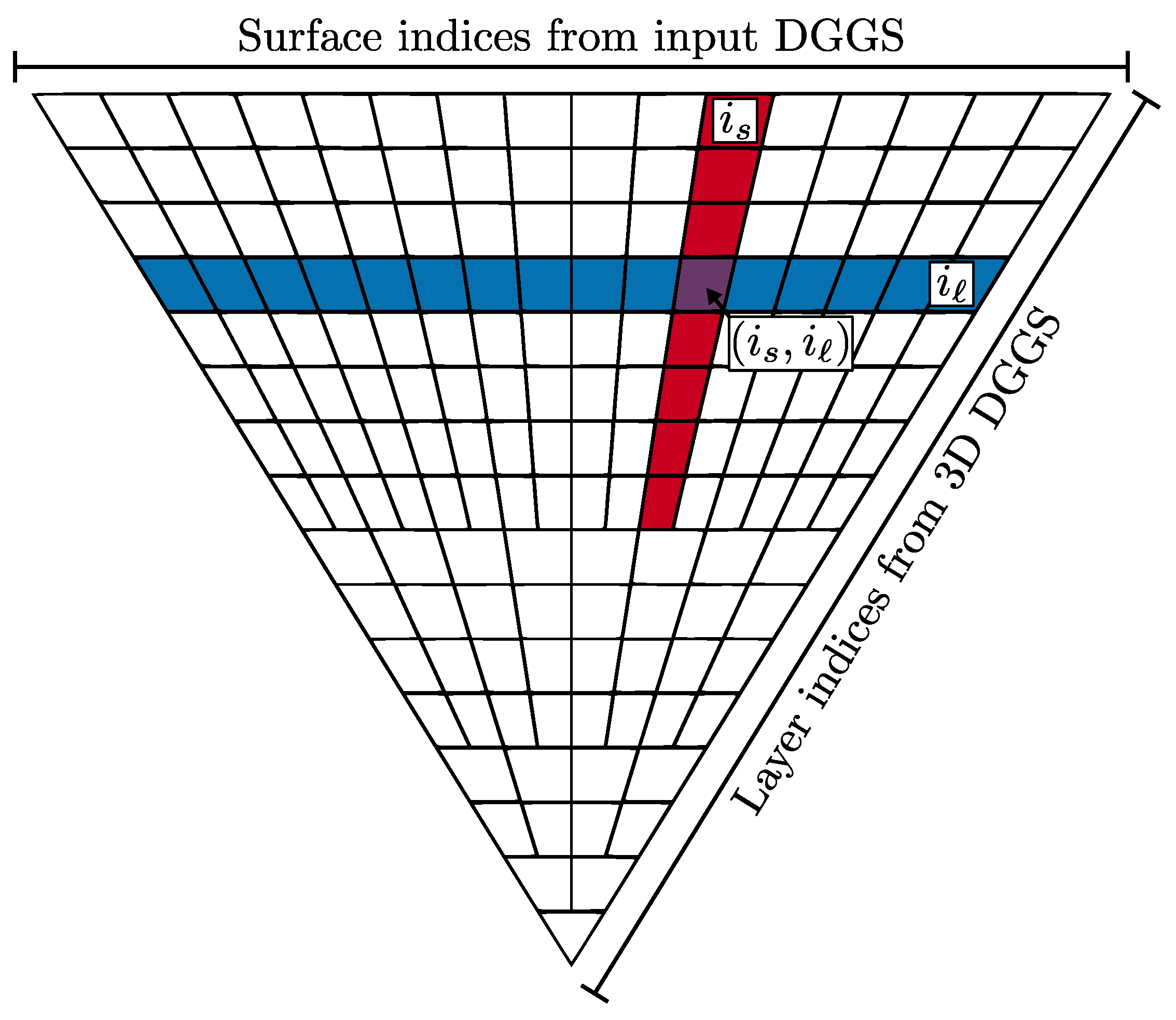
To accomplish this, we split encoding and decoding into a surface and radial component. Referring to Figure 9, we justify such a split by noting that two components define each cell in a 3D DGGS: the cell in the input DGGS that defines its base(s) and the layer of the grid that contains it. Uniquely identifying each of these components is sufficient to identify every cell in the grid uniquely; furthermore, each of these components is determined almost entirely independently.
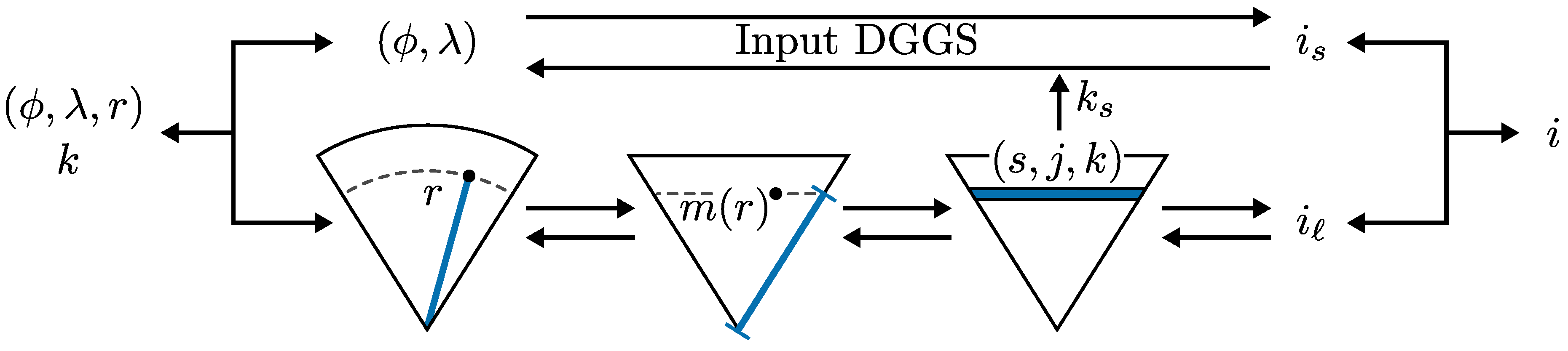
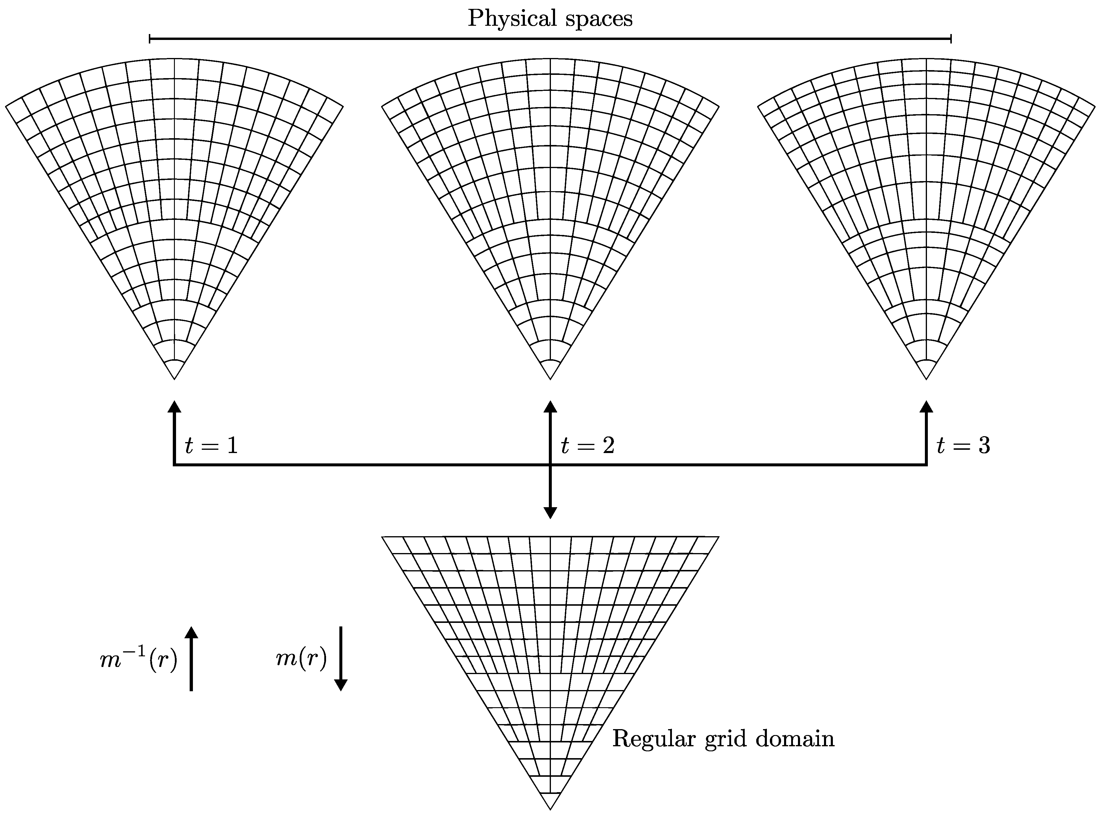
Our proposed split of these operations is depicted in Figure 10. The surface component of encoding/decoding is handled entirely by the input DGGS and therefore is not discussed here. For the radial component, we first introduce radial mapping functions, which map a physical radius, r, to a corresponding radius in the grid, . This function serves a similar purpose to the polyhedral projection of a conventional DGGS and allows for improved volume preservation between cells. We also provide operations for parameterizing the layers of a 3D DGGS and correspondingly finding the minimum and maximum grid radius of a layer from such a parameterization. We do not discuss methods for converting this parameterization into an index for the layer or for combining surface and layer indices into a single index. For the former, this is due to varying complexities of the layer structure in different 3D DGGS and competing goals in an efficient indexing system. For the latter, this operation depends heavily on the indexing structure of the input DGGS and, therefore, cannot easily be defined in general.
5.1. Radial Mapping
For many conventional DGGSs, area-preserving projections are used to ensure every cell in a certain resolution of the grid has the same area when mapped to the corresponding region of the Earth [19,21,48]. This property is important for applications where the area of cells is frequently used, as this can be expensive to compute. Therefore, for a 3D DGGS, it may also be desired for each cell to have equal volume, or as close to equal as possible. This can be accomplished with a radial mapping that controls how radii in physical space are mapped to corresponding radii in grid space. Such a radial mapping is not strictly required, in which case an identity map can be used. Using an identity reduces the computational load of encoding and decoding but gives no control over volume preservation in the grid.
In order for a mapping M to be volume-preserving, it is required that
for all subdomains D in the domain of M. However, if the volumes of cells in the grid domain are not equal (as is the case with our 3D DGGSs), then a volume-preserving mapping does not result in cells of equal volume. Instead, all cells should be inversely mapped to equal volume elements in the domain regardless of their volume in the grid. Formally,
for all cell combinations and .
Below we describe three different radial maps that are used for varying degrees of volume preservation between layers in the grid. The first two—which are identical to ones provided in [22]—are special cases of the more general third. Volume preservation between cells is also dependent on the projection and refinement of the input DGGS, and is therefore not discussed in general for our 3D DGGSs. In these mappings, we use to refer to a radius r normalized to the range of the grid ().
Shell-Volume Preserving Mapping
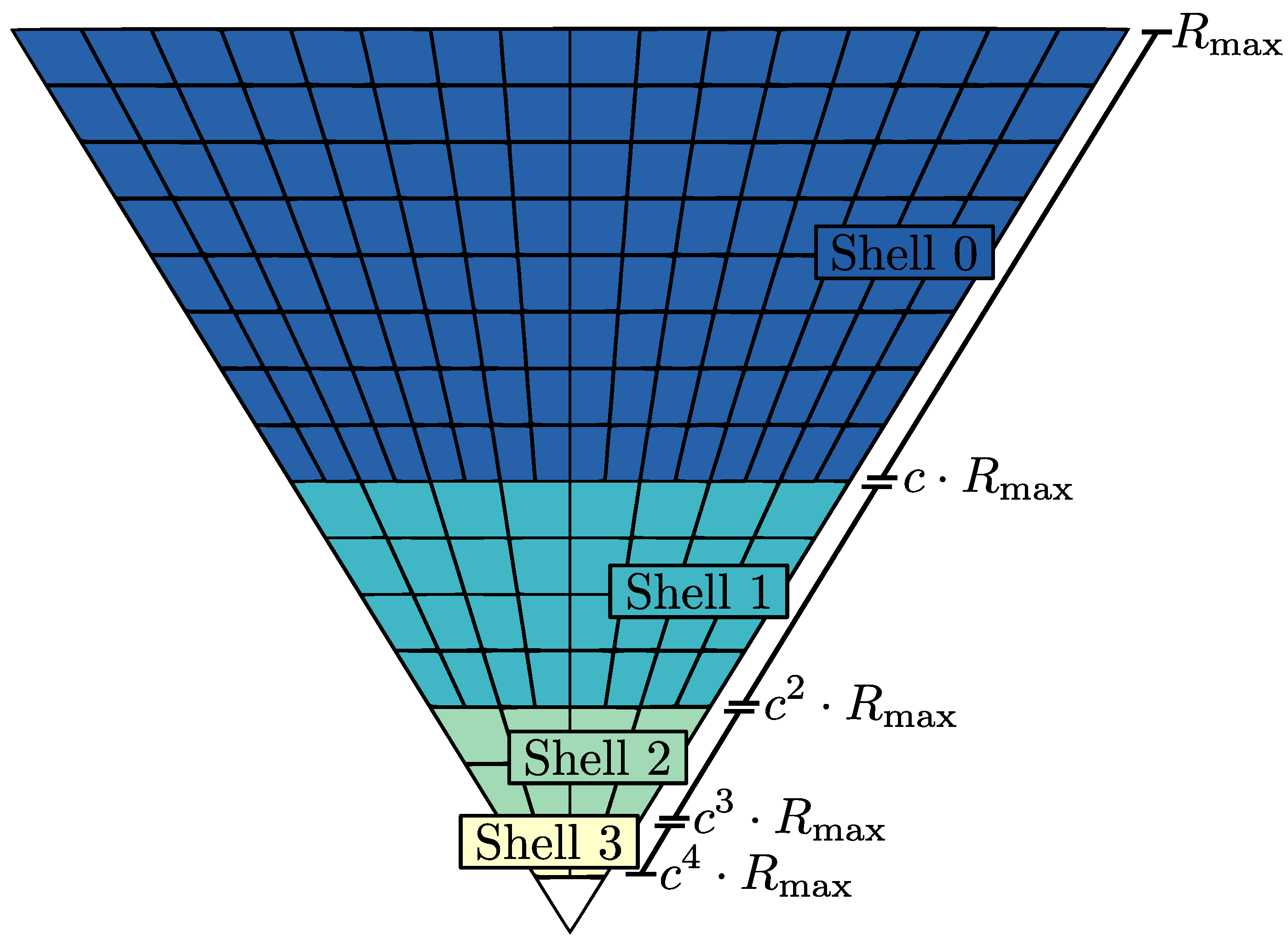
Referring to Figure 11, we see that the radial splits for central layers divide the grid into regions representing spherical shells. We also note that each of these shells contains a different number of cells. More specifically, shell n has a value of one greater than that of shell , and therefore as refinement continues, we expect shell n to contain times as many cells. Ideally, then, shell n will represent a region with times the volume as well. To accomplish this, we can define a radial mapping that maps radial splits in the grid to corresponding radial splits that result in the appropriate volume. We summarize the method below, with more details available in [22]. The volume shell n represents is proportional to
where is the distance along to map the radial splits to. Thus, the ratio of the volume between shell n and is
Equating this to the desired ratio of volumes, we get
From this, we conclude that radii at powers of c should be mapped to powers of ; radii that are in between are linearly interpolated. We first calculate the physical shell that contains the radius, which is simply . The shell is then used to find the (normalized) minimum and maximum radius of the shell in both physical and grid space. We refer to these as ℓ and u, respectively, with subscripts g for grid space and p for physical. These are given by
In the case that only regular prismatoid refinement is used, they are instead
The full mapping is thus
For the inverse, we have
For the inverse, shell s would be carried forward from the layer parameterization (Section 5.2), however it can also be calculated independently with .
The results of this mapping are shown in Figure 12 left. Note that for a 1:4 surface refinement factor, , which means this mapping is equivalent to the identity. In the case where only regular prismatoid refinement is used, this mapping is also equivalent to the identity.
This mapping—and the subsequent ones—have the side effect of changing the aspect ratio of cells in grid space as compared to the corresponding cells in physical space. This means that when determining the refinement parameters needed to achieve the desired aspect ratio, the cells in physical space should be considered as opposed to grid space, as done in Section 4.5. This is easily addressed by changing the value of used in Equations (1) and (2) to be .
Volume Preserving Mapping
While the above mapping preserves volume between shells of the grid, cells within a given shell will still have varying volumes. This is due to the volume of cells growing cubically with respect to radius. To accommodate this, we replace the linear interpolation of the above mapping with one that maps changes in volume in physical space to linear distance in grid space, the result of which is
Likewise, the inverse is given by
With this mapping, cells in the same layer will have perfect volume preservation assuming the input DGGS is area preserving. Depending on the layering sequence, however, volume will not necessarily be preserved between cells in different shells. Additionally, the centre layer will never have volume preservation with the other layers. The results of this mapping are shown in Figure 12 right. As can be seen, cells in each shell are stretched and squashed in order to ensure they have equal volume.
Balanced Mapping
While volume preservation is an important property for certain applications, it may also be desirable to avoid the stretching and squashing noted above. To accommodate different balances of volume preservation and cell compactness, we use a mapping that blends between the results of the first and second proposed mappings. Mapping one uses linear interpolation, and results in cells with equal radial extent; mapping two uses a cubic interpolation and results in cells with equal volume. Using a different power, t, between one and three will result in a blending between these two properties. A result using is shown in Figure 12 centre.
5.2. Layer Parameterization
Layers of a 3D DGGS can be parameterized by the shell they are in (s), the integer index of the layer relative to the shell (j), and the level of refinement (k). The shell carries forward from the above radial mappings or can be recalculated in the same manner, and the level of refinement is an input into the encoding process. Thus, all that remains is the integer index.
In order to calculate the integer index of a layer, the number of layers in the shell is first needed. The number of layers in a shell depends on the refinement level, the layering sequence, and the number of extra radial splits (see Section 4.5). Once again, the level of refinement is an input and the other variables are constant for any given 3D DGGS. Therefore, the number of layers, , is given by
In the case where s is greater than or equal to , the shell is in the central layer. In this case, we set and note that there is only one layer in the shell. The integer index of the layer is then , where d is carried forward from the radial mapping or independently calculated in the same manner. Finally, as input into the surface encoding, the value of is needed for the shell. For central layers, this is always zero; otherwise, it is given by .
For decoding, we calculate and as and respectively, which is then fed directly into the inverse mapping as values of d.
6. Indexing Operations
An important component of a conventional DGGS is the indexing scheme for cells. Indices in a DGGS are used to not only identify and linearize cells but also as a means of navigating the grid for various spatial queries [11]. To this end, it is important to be able to perform certain operations on said indices efficiently. The most fundamental of these operations are parent queries, which return the parent (or with non-congruent refinement, parents) of a given cell; child queries, which return the children of the cell; and neighbour queries, which return cells that share an edge (or in 3D a face) with the cell. These operations serve as the building blocks for more complex geospatial queries done with the grid system, such as region growing, data convolution and correlation, feature rasterization, and buffering. Because of this, creating suitable indexing for a 3D DGGS is an essential task.
With our method—similar to encoding and decoding—we define these operations in terms of surface and radial components. This split not only simplifies the problem of indexing but also ensures the 3D indexing is consistent with that of the input DGGS. Referring back to Figure 9 and Figure 10, we let be the surface index of a cell and be the layer index. For each of these components, we assume there is a corresponding parent, child, and neighbour operation. For the surface index, this comes directly from the input DGGS indexing, whereas for the layer index, these would need to be defined. Using the component operations, we define the corresponding 3D operations as follows.
Parents
The parent(s) of a cell depends on if the layer of the cell and its parent layer have the same or different values of . Let ; if the value of is the same, then the single parent is simply . In most cases, the value of for is some number m (often one, but not always) less than that of . In this case, the parent(s) are given by .
Children
The Children of a Cell Depend on if the Cell Belongs to a Central or Normal Layer For normal layers, the set of children is simply . For central layers, the child who belongs to the new central layer must be distinguished from the other child layer(s). Call the index of the new central layer ; then, this child is given by . Let give the set of the other children layer indices (normal layers). These layers have the surface refinement applied w times, so the resulting children are
Neighbours
We split neighbours into three categories: neighbours in the same layers as the cell, neighbours in the layer above the cell, and neighbours in the layer below the cell. If a cell belongs to the outermost or innermost (central) layer, then it will not have neighbours in the layer above or below, respectively. Neighbours in the same layer are simply . Let be the layer above and be the layer below. If has the same value of as , then the single neighbour above is . In the other case, where the value of for is some number m greater than that of , the neighbours are given by . Likewise, if has the same value of as , there is one neighbour below given by . In the case that the value of for is some number m less than that of , the neighbours are given by .
7. Results and Evaluation
To evaluate our approach, we have implemented the general method described in the previous sections as a C++ class integrated with a research toolset used for designing and testing different conventional DGGSs. In this toolset, the operations provided by a DGGS are specified by an abstract class that each implementation extends. The 3D DGGS class takes an input DGGS as well as values for the target aspect ratio (a), exponent for the radial mapping (t), and the radial range of the grid ( and ) as input during construction. The 3D DGGS uses these values—along with the operations and information provided by the input DGGS—to provide the functionality described in the paper: point encoding, cell decoding, parents, children, and neighbours. We also provide the ability to create basic visualization of the grid. These visualizations were used as a basis for many of the figures in this paper.
We evaluate our system by looking at three sample use cases for our 3D DGGSs. These use cases are not meant to be state-of-the-art implementations of a 3D global grid system, but rather are meant to demonstrate the robustness and versatility of the approach and its ability to support different target applications, data sets, and input DGGSs. For each use case, we chose an input DGGS and parameters for the system that resulted in a 3D DGGS with desirable properties for said application. The data encodings in these use cases are all defined using the fundamental operations of the 3D DGGS listed above.
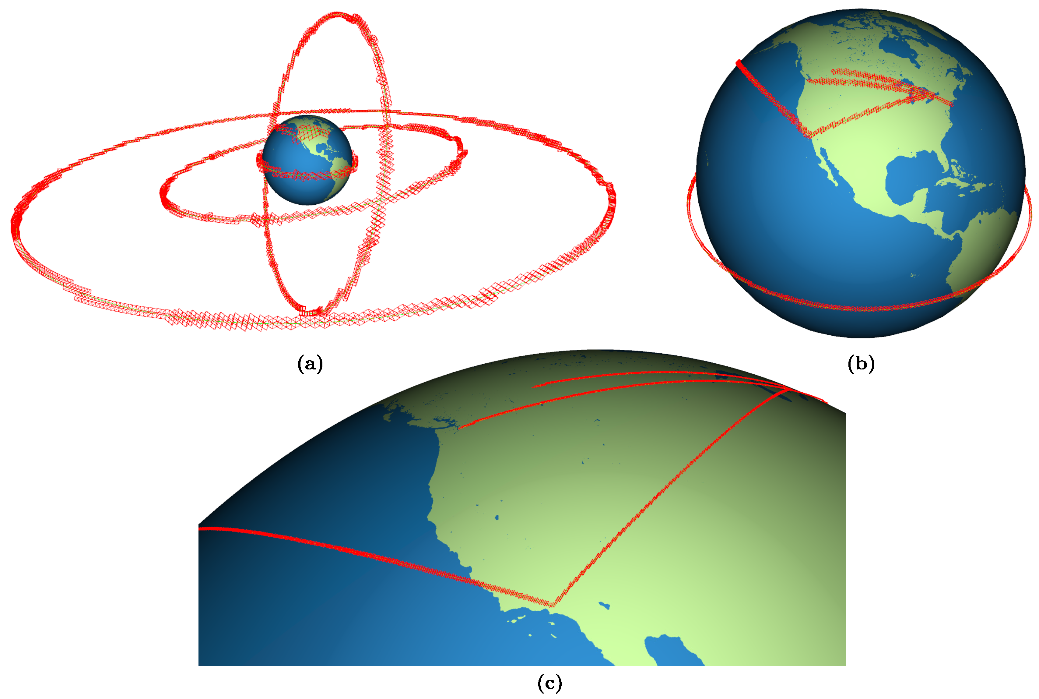
7.1. Aircraft and Satellite Paths
The first use case we examine is tracking the trajectories of aircraft and spacecraft, such as commercial and private flights, drones, satellites, and rockets. Such a system could be used to increase the efficiency of collision queries using the hierarchy of the grid system, similar to the approaches of [34,35]. The main benefit our 3D DGGS would offer over existing grids for such a system is the ability to have cells located at low and high altitudes in the same resolution have close to equal shape and size.
Figure 13 shows several generated flight paths and satellite orbits represented in a 3D DGGS at increasing resolutions. The input DGGS for this example uses a rhombic triacontahedron as the initial polyhedron, standard 1:4 quadrilateral refinement, and a simple normalization projection. The 3D DGGS has a target aspect ratio of one, a radial mapping exponent of one, and a radial range of 10.66R (67,957 km). These parameters were chosen to ensure that cells are as compact as possible.
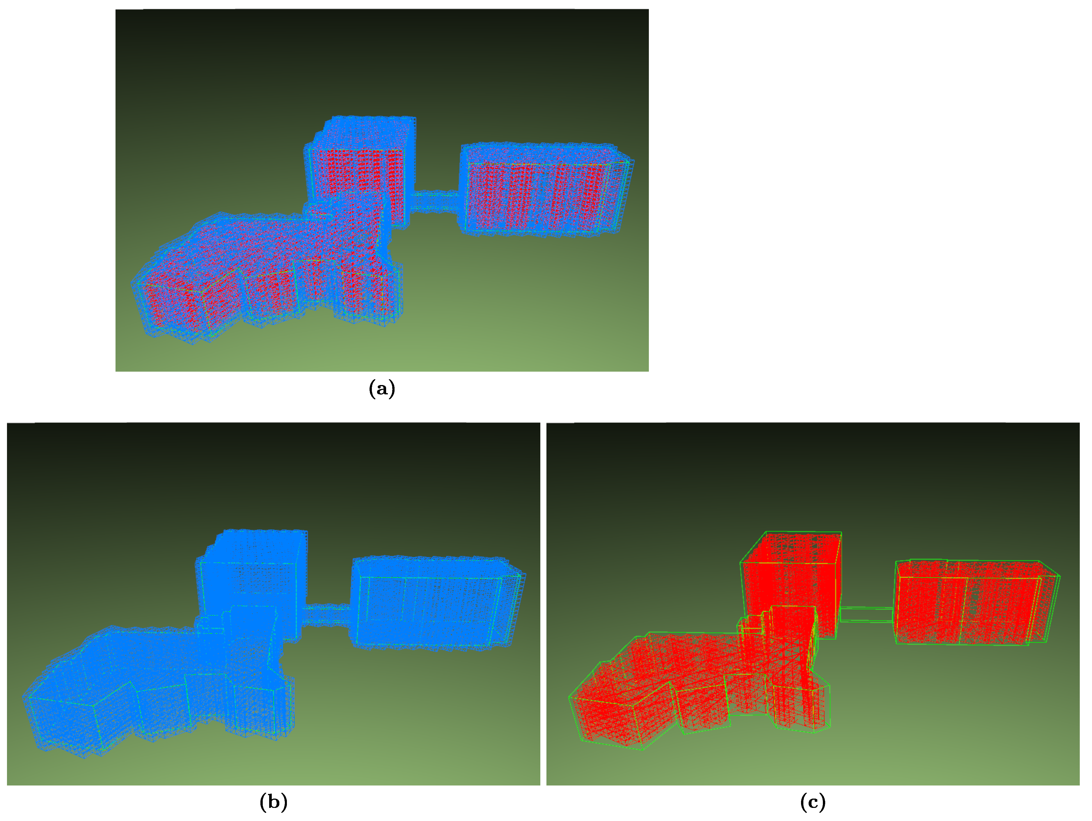
7.2. Urban Planning
The second use case is a volume-preserving 3D grid for the purpose of urban planning and management. A volume-preserving grid is useful for quickly estimating the volume of a feature rasterized in the grid by multiplying the number of cells by their volume. This use case also shows the ability of our 3D DGGS to handle small scale data in addition to the much larger scale data showcased in Section 7.1.
Figure 14 shows several buildings represented in a 3D DGGS, with the building geometries obtained from Open Street Map [49]. The input DGGS for this example uses a disdyakis triacontahedron as the initial polyhedron, a non-standard 1:4 triangle refinement, and the vertex oriented great circle slice and dice projection [48] to preserve area [50]. The 3D DGGS has a target aspect ratio of one, a radial mapping exponent of three to achieve perfect volume preservation (excluding the central layer), and a maximum radius of 1.33R (8495 km).
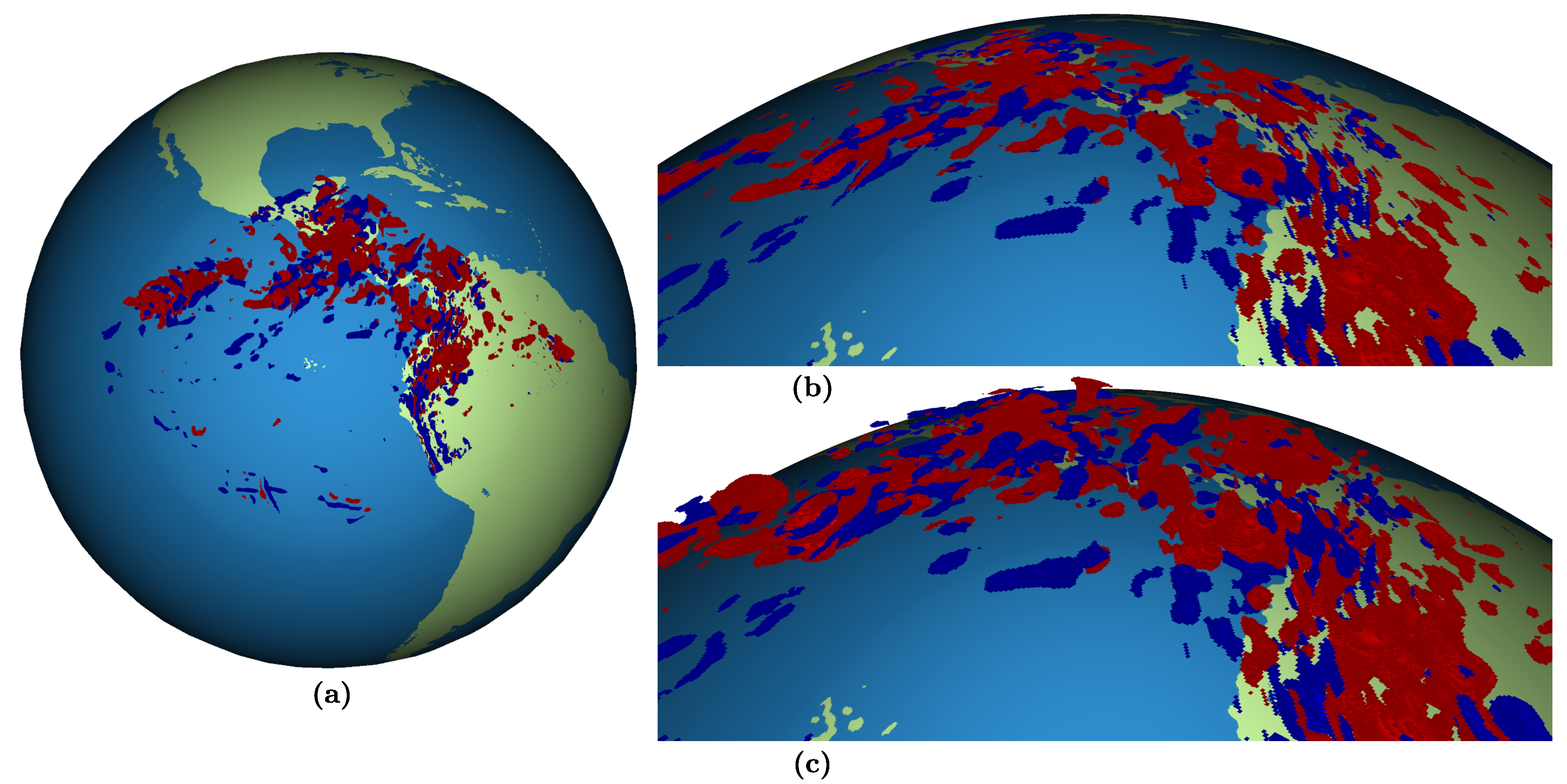
7.3. Atmospheric Properties
The final use case we look at is using a 3D DGGS to resample atmospheric forecasts, such as those generated by numerical weather prediction models. These datasets typically have a much higher vertical resolution than surface resolution, due to how quickly properties such as temperature and wind speed tend to change in these two dimensions. To accommodate this with our 3D DGGS, we specify an appropriate aspect ratio for cells to ensure the vertical and surface resolution matches as closely as possible that of the input data.
Figure 15 shows vertical wind speed from the ERA5 dataset [51] sampled into a 3D DGGS. The input DGGS for this example is the same as the one used for the aircraft and satellite paths. However, this 3D DGGS has a target aspect ratio of 31.7, a radial mapping exponent of one, and a maximum radius of 1.33R (8495 km).
7.4. Discussion
The above examples are only a small subset of the many potential applications of our 3D DGGSs. Despite this, they show not only the useful properties achievable by the method (support for large ranges of altitudes, volume preservation between cells, custom cell aspect ratio, and support for multiple scales of data) but also demonstrate the ease at which new 3D global grids can be created. Given a conventional DGGS that provides the required operations, creating a 3D DGGS is as simple as providing the surface grid and four clearly defined parameters for the 3D one. Since creating a 3D DGGS that is ideal for every application is not possible, this allows quick iterations on creating and comparing different 3D grids to find the ideal one for each application.
8. Conclusions and Future Work
With the amounts of 3D geospatial data becoming available, techniques for integrating and managing such data are becoming increasingly important. To this end, we have proposed a complete and comprehensive method for extending any DGGS to 3D for use as a 3D global grid system. Our approach is general, and properly accommodates any potential DGGS regardless of the initial polyhedron, refinement, or projection employed. Semiregular refinement is used to allow large radial ranges to be represented without significant degradation in cell shape or size. Techniques are employed to ensure cells have the desired aspect ratio, and that the aspect ratio and relative volumes of cells are maintained during refinement. We also provide a pipeline to handle encoding and decoding of these grids in a manner which facilitates simple data transference between the 2D and 3D representations. As a part of this, we derive a class of radial mappings that achieve varying degrees of volume preservation in the grid. The effectiveness of this framework is showcased in three sample use cases, each using a different 3D DGGS explicitly tailored for the needs of the application.
There are still some important future works to be done. While we have provided tools that can be used to develop an indexing scheme for a 3D DGGSs, a more detailed exploration of the topic—especially methods for interleaving surface and layer indices for locality—is necessary. The methods developed for combining these indices could also be extended to the time dimension and may serve as the basis for developing better techniques for time-varying DGGS. Also, while most DGGSs use a sphere as the reference model of the Earth, an oblate spheroid provides a more accurate representation. While we suspect our method is just as applicable to an ellipsoidal DGGS, more research is required to justify this claim and address any necessary changes to the method.
Other directions for future work include defining more efficient high-level operations for operating with a 3D DGGS. Insertion and rasterization of features such as 3D vectors, models, and meshes are important operations for a 3D grid, and the algorithms currently used for this with our 3D DGGS are quite basic. There may also be ways for the structure of a 3D DGGS to aid in occlusion issues that appear in certain visualization. Slice views and rendering of select layers may prove to be a useful tool in visualizing subterranean data and other datasets with significant occlusion.
Author Contributions
Conceptualization, Faramarz Samavati; Funding acquisition, Faramarz Samavati; Investigation, Benjamin Ulmer; Methodology, Benjamin Ulmer and John Hall; Project administration, Faramarz Samavati; Software, Benjamin Ulmer and John Hall; Supervision, Faramarz Samavati; Visualization, Benjamin Ulmer; Writing—original draft, Benjamin Ulmer; Writing—review & editing, John Hall and Faramarz Samavati. All authors have read and agreed to the published version of the manuscript.
Funding
This research was partially funded by the Natural Sciences and Engineering Research Council of Canada (NSERC).
Acknowledgments
We wish to thank Lakin Wecker for insightful technical discussion and Troy Alderson for editorial comments.
Conflicts of Interest
The authors declare no conflict of interest.
Abbreviations
The following abbreviations are used in this manuscript:
| GIS | Geographic Information System |
| DGGS | Discrete Global Grid System |
| 3D DGGS | Three-dimensional Discrete Global Grid System |
References
- Lee, J.G.; Kang, M. Geospatial Big Data: Challenges and Opportunities. Big Data Res. 2015, 2, 74–81. [Google Scholar] [CrossRef]
- Antenucci, J.C.; Brown, K.; Croswell, P.L.; Kevany, M.J.; Archer, H. Geographic Information Systems: A Guide to the Technology; Van Nostrand Reinhold: New York, NY, USA, 1991. [Google Scholar]
- Foresman, T.W. The History of Geographic Information Systems: Perspectives from the Pioneers; Vol. 397; Prentice Hall: Upper Saddle River, NJ, USA, 1998. [Google Scholar]
- Hennerdal, P. Beyond the Periphery: Child and Adult Understanding of World Map Continuity. Ann. Assoc. Am. Geogr. 2015, 105, 773–790. [Google Scholar] [CrossRef]
- Hruby, F.; Avelino, M.C.; Ayala, R.M. Journey to the End of the World Map–How Edges of World Maps Shape the Spatial Mind. J. Geogr. Inf. Sci. 2016, 1, 314–323. [Google Scholar] [CrossRef] [Green Version]
- Flater, D. Understanding Geodesic Buffering. Available online: https://www.esri.com/news/arcuser/0111/geodesic.html (accessed on 23 January 2020).
- Wang, Y.; Liu, Z.; Liao, H.; Li, C. Improving the Performance of GIS Polygon Overlay Computation with MapReduce for Spatial Big Data Processing. Cluster Comput. 2015, 18, 507–516. [Google Scholar] [CrossRef]
- Sahr, K.; White, D. Discrete Global Grid Systems. Comp. Sci. Stat. 1998, 269–278. [Google Scholar]
- Mahdavi-Amiri, A.; Alderson, T.; Samavati, F. A Survey of Digital Earth. Comput. Graph. 2015, 53, 95–117. [Google Scholar] [CrossRef]
- OGC (2017a). Discrete Global Grid Systems Abstract Specification. Available online: http://docs.opengeospatial.org/as/15-104r5/15-104r5.html (accessed on 2 August 2018).
- Alderson, T.; Purss, M.; Du, X.; Mahdavi-Amiri, A.; Samavati, F. Digital Earth Platforms. In Manual of Digital Earth; Springer: Berlin/Heidelberg, Germany, 2020; pp. 25–54. [Google Scholar]
- Yoo, J.S.; Min, K.J.; Ahn, J.W. Concept and Framework of 3D Geo-Spatial Grid System. International Symposium on Web and Wireless Geographical Information Systems; Springer: Berlin/Heidelberg, Germany, 2019; pp. 136–149. [Google Scholar]
- Yu, J.Q.; Wu, L.X. Spatial Subdivision and Coding of a Global Three-Dimensional Grid: Spheoid Degenerated-Octree Grid. In Proceedings of the Geoscience and Remote Sensing Symposium, Cape Town, South Africa, 12–17 July 2009; Volume 2, pp. 2–361. [Google Scholar]
- Gang, W.; Xuefeng, C.; Feng, L.; Ke, L. Sphere Shell Space 3D Grid. Int. Arch. Photogramm. Remote Sens. Spatial Inf. Sci. 2013, 40, 77–82. [Google Scholar] [CrossRef] [Green Version]
- Sun, Z.; Cheng, C. 3D Integrated Representation Model and Visualization Based on the Global Discrete Voxel—GeoSOT3D. In Proceedings of the 2015 23rd International Conference on Geoinformatics, Wuhan, China, 19–21 June 2015; pp. 1–5. [Google Scholar]
- Fekete, G.; Treinish, L.A. Sphere Quadtrees: A New Data Structure to Support the Visualization of Spherically Distributed Data. In Proceedings of the Extracting Meaning from Complex Data: Processing, Display, Interaction, Santa Clara, CA, USA, 11–16 February 1990; Volume 1259, pp. 242–253. [Google Scholar] [CrossRef]
- Dutton, G. Encoding and Handling Geospatial Data with Hierarchical Triangular Meshes. In Proceedings of the 7th Symposium on Spatial Data Handling; Taylor & Francis: Abingdon, UK, 1996; Volume 43, pp. 505–518. [Google Scholar]
- Gorski, K.M.; Hivon, E.; Banday, A.J.; Wandelt, B.D.; Hansen, F.K.; Reinecke, M.; Bartelmann, M. HEALPix: A Framework for High-Resolution Discretization and Fast Analysis of Data Distributed on the Sphere. Astrophys. J. 2005, 622, 759. [Google Scholar] [CrossRef]
- Holhoş, A.; Roşca, D. An Octahedral Equal Area Partition of the Sphere and Near Optimal Configurations of Points. Comput. Math. Appl. 2014, 67, 1092–1107. [Google Scholar] [CrossRef]
- Snyder, J.P. Map Projections–A Working Manual; US Government Printing Office: Washington, DC, USA, 1987; Volume 1395.
- Snyder, J.P. An Equal-Area Map Projection for Polyhedral Globes. Cartographica 1992, 29, 10–21. [Google Scholar] [CrossRef]
- Ulmer, B.; Samavati, F. Toward Volume Preserving Spheroid Oegenerated-Octree Grid. GeoInformatica 2020, 1–25. [Google Scholar]
- Bahrdt, D.; Seybold, M.P. Rational Points on the Unit Sphere: Approximation Complexity and Practical Constructions. In Proceedings of the 2017 ACM on International Symposium on Symbolic and Algebraic Computation, Kaiserslautern, Germany, 25–28 July 2017; pp. 29–36. [Google Scholar]
- Alderson, T.; Mahdavi-Amiri, A.; Samavati, F. Multiresolution on Spherical Curves. Graph. Models 2016, 86, 13–24. [Google Scholar] [CrossRef]
- Alderson, T.; Samavati, F. Multiscale NURBS Curves on the Sphere and Ellipsoid. Comput. Graph. 2019, 82, 243–249. [Google Scholar] [CrossRef]
- Alderson, T.; Mahdavi-Amiri, A.; Samavati, F. Offsetting Spherical Curves in Vector and Raster Form. Visual Comput. 2018, 34, 973–984. [Google Scholar] [CrossRef]
- Goodchild, M.F. Reimagining the History of GIS. Ann. GIS 2018, 24, 1–8. [Google Scholar] [CrossRef]
- Sahr, K.; White, D.; Kimerling, A.J. Geodesic Discrete Global Grid Systems. Cartogr. Geogr. Inf. Sci. 2003, 30, 121–134. [Google Scholar] [CrossRef] [Green Version]
- Vince, A. Indexing the Aperture 3 Hexagonal Discrete Global Grid. J. Vis. Commun. Image Represent. 2006, 17, 1227–1236. [Google Scholar] [CrossRef]
- Tong, X.; Ben, J.; Wang, Y.; Zhang, Y.; Pei, T. Efficient Encoding and Spatial Operation Scheme for Aperture 4 Hexagonal Discrete Global Grid System. Int. J. Geogr. Inf. Sci. 2013, 27, 898–921. [Google Scholar] [CrossRef]
- Du, L.; Ma, Q.; Ben, J.; Wang, R.; Li, J. Duality and Dimensionality Reduction Discrete Line Generation Algorithm for a Triangular Grid. ISPRS Int. J. Geoinf. 2018, 7, 391. [Google Scholar] [CrossRef] [Green Version]
- Mahdavi-Amiri, A.; Samavati, F.; Peterson, P. Categorization and Conversions for Indexing Methods of Discrete Global Grid Systems. ISPRS Int. J. Geoinf. 2015, 4, 320–336. [Google Scholar] [CrossRef]
- Sirdeshmukh, N.; Verbree, E.; Oosterom, P.V.; Psomadaki, S.; Kodde, M. Utilizing a Discrete Global Grid System for Handling Point Clouds with Varying Locations, Times, and Levels of Detail. Cartographica 2019, 54, 4–15. [Google Scholar] [CrossRef] [Green Version]
- Miao, S.; Cheng, C.; Zhai, W.; Ren, F.; Zhang, B.; Li, S.; Zhang, J.; Zhang, H. A Low-Altitude Flight Conflict Detection Algorithm Based on a Multilevel Grid Spatiotemporal Index. ISPRS Int. J. Geoinf. 2019, 8, 289. [Google Scholar] [CrossRef] [Green Version]
- Zhai, W.; Tong, X.; Miao, S.; Cheng, C.; Ren, F. Collision Detection for UAVs Based on GeoSOT-3D Grids. ISPRS Int. J. Geoinf. 2019, 8, 299. [Google Scholar] [CrossRef] [Green Version]
- Bassin, C. The Current Limits of Resolution for Surface Wave Tomography in North America. EOS Trans. AGU. 81: Fall Meet. Suppl. Abstract 2000, 81, F897. [Google Scholar]
- Zhao, D. Global Tomographic Images of Mantle Plumes and Subducting Slabs: Insight into Deep Earth Dynamics. Phys. Earth Planet. Inter. 2004, 146, 3–34. [Google Scholar] [CrossRef]
- Kageyama, A.; Sato, T. “Yin-Yang grid”: An Overset Grid in Spherical Geometry. Geochem. Geophys. Geosyst. 2004, 5. [Google Scholar] [CrossRef] [Green Version]
- Yoshida, M.; Kageyama, A. Application of the Yin-Yang Grid to a Thermal Convection of a Boussinesq Fluid with Infinite Prandtl Number in a Three-Dimensional Spherical Shell. Geophys. Res. Lett. 2004, 31. [Google Scholar] [CrossRef] [Green Version]
- Kageyama, A.; Yoshida, M. Geodynamo and Mantle Convection Simulations on the Earth Simulator using the Yin-Yang Grid. J. Phys. 2005, 16, 325. [Google Scholar] [CrossRef] [Green Version]
- Tackley, P.J. Modelling Compressible Mantle Convection with Large Viscosity Contrasts in a Three-Dimensional Spherical Shell using the Yin-Yang Grid. Phys. Earth Planet. Inter. 2008, 171, 7–18. [Google Scholar] [CrossRef]
- Yu, J.; Wu, L. On Coding and Decoding for Sphere Degenerated-Octree Grid. Geogr. Geo-Inf. Sci. 2009, 25, 5–9. [Google Scholar]
- Yu, J.; Wu, L.; Li, Z.; Li, X. An SDOG-Based Intrinsic Method for Three-Dimensional Modelling of Large-Scale Spatial Objects. Ann. GIS 2012, 18, 267–278. [Google Scholar] [CrossRef]
- Yu, J.; Wu, L.; Zi, G.; Guo, Z. SDOG-Based Multi-Scale 3D Modeling and Visualization on Global Lithosphere. Sci. China Earth Sci. 2012, 55, 1012. [Google Scholar] [CrossRef]
- Holhoş, A.; Roşca, D. Uniform Refinable 3D Grids of Regular Convex Polyhedrons and Balls. Acta Math. 2018, 156, 182–193. [Google Scholar] [CrossRef]
- Holhoş, A.; Roşca, D. Area Preserving Maps and Volume Preserving Maps Between a Class of Polyhedrons and a Sphere. Adv. Comput. Math. 2017, 43, 677–697. [Google Scholar] [CrossRef] [Green Version]
- Xie, J.; Yu, H.; Ma, K.L. Interactive Ray Casting of Geodesic Grids. In Computer Graphics Forum; Wiley: Hoboken, NJ, USA, 2013; Volume 32, pp. 481–490. [Google Scholar]
- van Leeuwen, D.; Strebe, D. A “Slice-and-Dice” Approach to Area Equivalence in Polyhedral Map Projections. Cartogr. Geogr. Inf. Sci. 2006, 33, 269–286. [Google Scholar] [CrossRef]
- OpenStreetMap Contributors. Open Street Map. Available online: https://www.openstreetmap.org/ (accessed on 27 January 2020).
- Hall, J.; Wecker, L.; Ulmer, B.; Samavati, F. Disdyakis Triacontahedron DGGS. manuscript in preparation.
- Copernicus Climate Change Service Climate Data Store (CDS). Copernicus Climate Change Service (C3S) (2017): ERA5: Fifth Generation of ECMWF Atmospheric Reanalyses of the Global Climate. Available online: https://cds.climate.copernicus.eu/cdsapp (accessed on 4 October 2019).
Figure 1.
Overview of how the input Discrete Global Grid System (DGGS) is used to define the geometry of the three-dimensional (3D) DGGS. The faces of the initial polyhedron of the input DGGS are first extruded to create the prismatoid base cells of the 3D DGGS. For refinement, the bases of these prismatoid cells are refined using the same refinement scheme as the input DGGS and combined with a radial refinement. A semiregular refinement is suggested; however, regular refinement is also possible. A more detailed description of these processes is provided in Section 4.
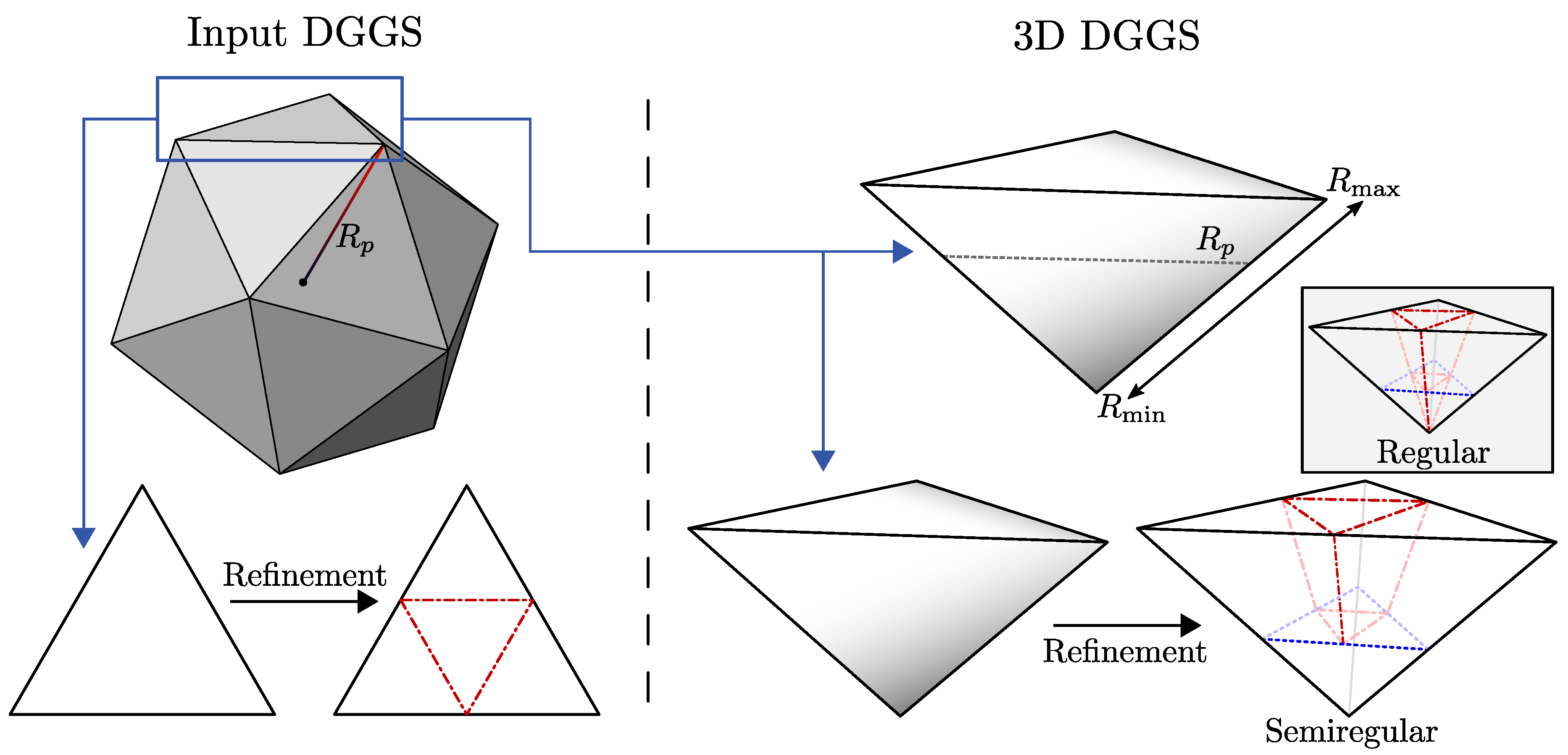
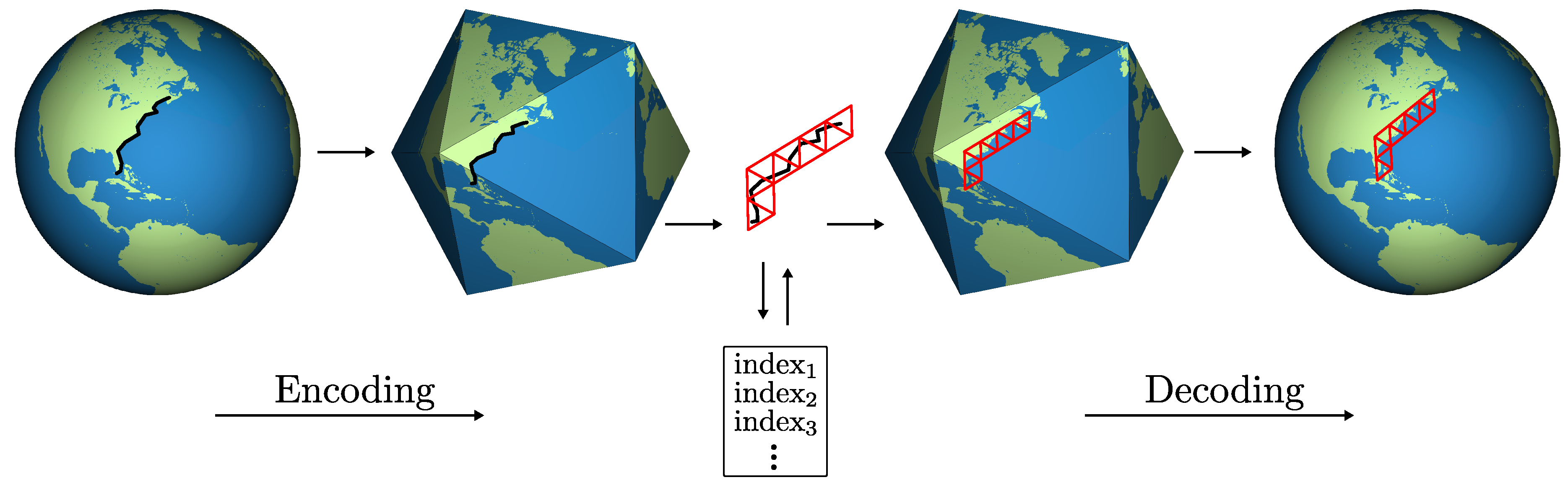
Figure 2.
The process of encoding (left) and decoding (right) with a DGGS. Encoding: features are projected from the Earth domain to the polyhedral domain of the grid; the set of planar cells associated with the feature are obtained—each of which has a unique index. Decoding: a set of cell indices corresponds to cell geometry on the polyhedral grid; cells in the polyhedral domain are inverse projected back to the Earth domain. The process for a 3D DGGS is similar, except features and cells have associated altitude(s).

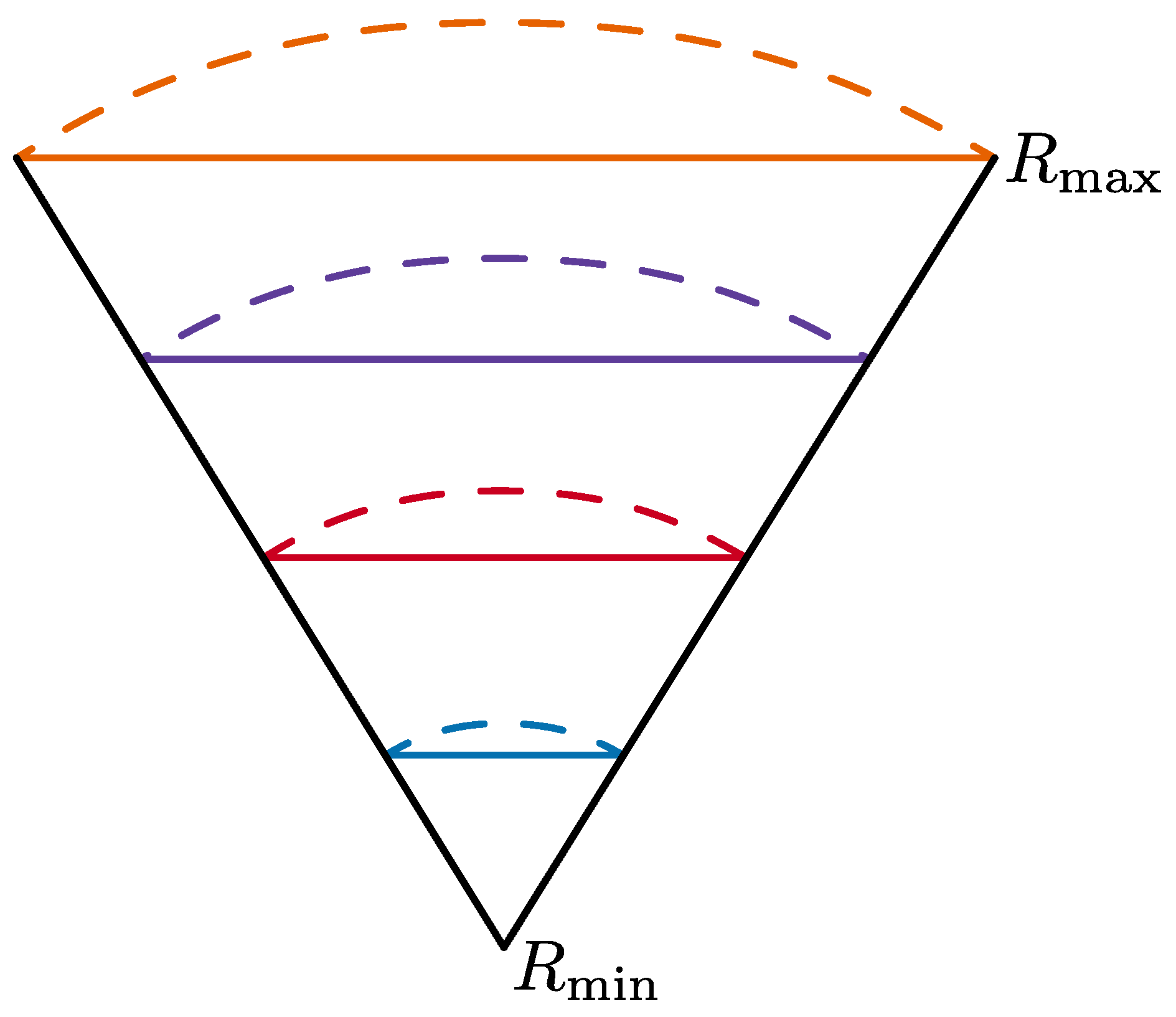
Figure 3.
The radius of a polyhedron is defined as the radius of its circumscribing sphere. In this figure, all points on a solid line of a given colour have the same radius as they all have the same circumscribing sphere (i.e., lie on the same polyhedron). The corresponding spheres are shown in the same colours but with a dashed line.

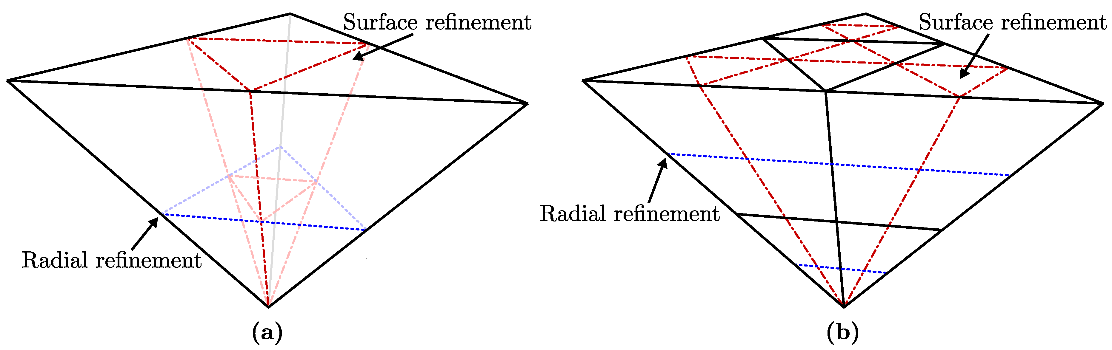
Figure 4.
Regular prismatoid refinement as applied to a single pyramid cell (a) once and (b) twice.

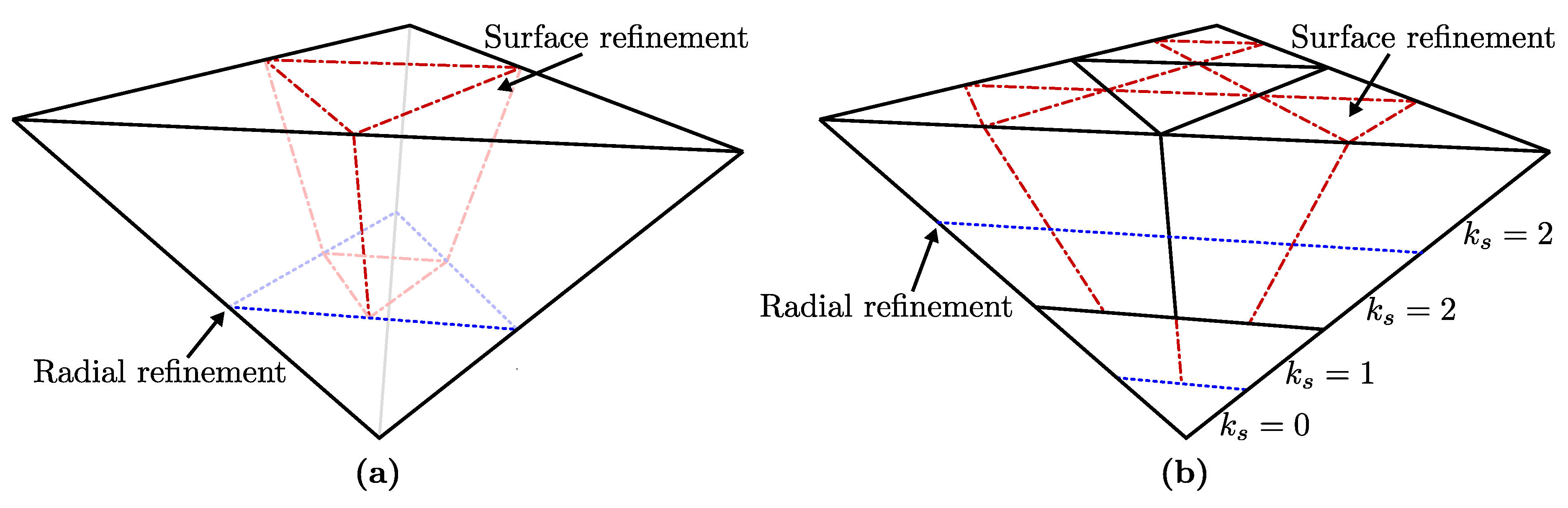
Figure 5.
Semiregular prismatoid refinement as applied to a single pyramid cell (a) once and (b) twice. In (b), the number of times the surface refinement has been applied () is shown for each layer; see how the radial refinements of central layers separate regions of the grid with different values of .

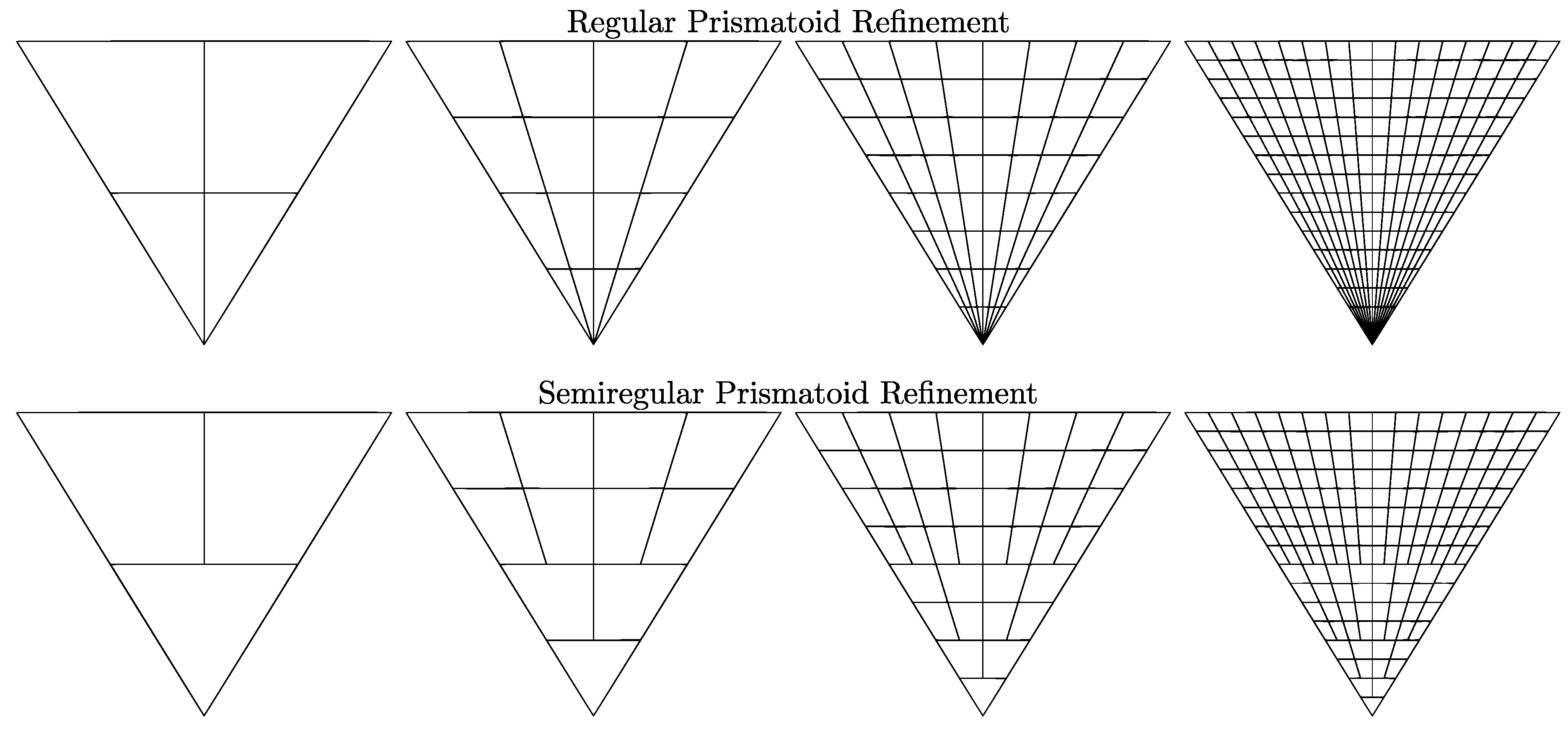
Figure 6.
Three levels of successive applications of regular (top) and semiregular (bottom) prismatoid refinement. Only the side of a single pyramid starting cell is shown to highlight the behaviour of the two schemes at different radii. Note how cells degenerate towards the centre with regular refinement, whereas this issue is not present in the semiregular scheme.

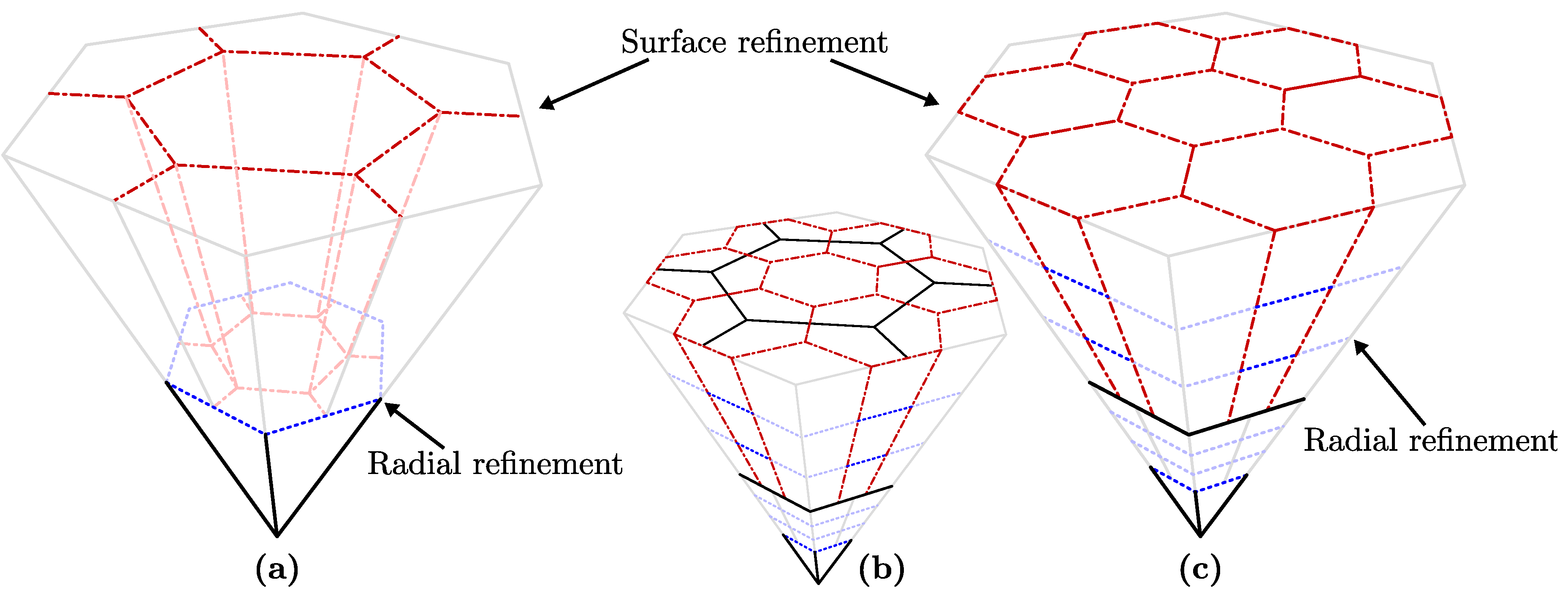
Figure 7.
Semiregular prismatoid refinement applied to a hexagonal base cell using a 1:3 surface refinement scheme (a) once and (c) twice; (b) is the same image as (c), but with the surface cells of the previous refinement level shown for reference. Note that in the second level of refinement, normal layers have two radial refinements as opposed to one.

Figure 8.
A demonstration of how refinement can be modified to affect the aspect ratio of cells. All figures show a starting pyramid cell from a grid with 200 cells in its initial discretization. Central layer with five extra radial splits (a = 3 to get x = 5) at (a) one level of refinement and (b) three levels. Central layer with two applications of the surface refinement scheme (a = 1/8 to get w = 2) at (c) one level of refinement and (d) three levels.
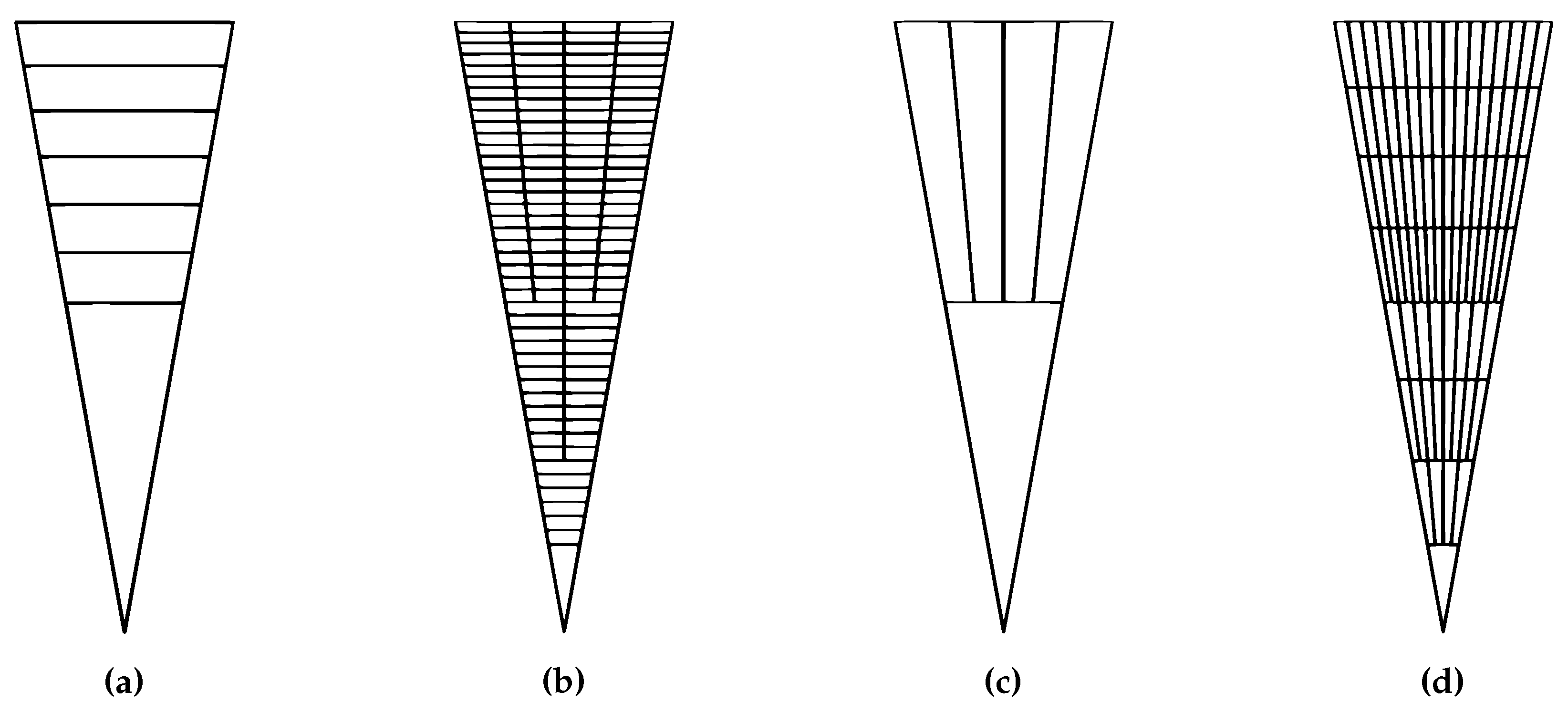
Figure 9.
Indices from the input DGGS identify cells in the 3D DGGS with the same bases but different radii. Likewise, each layer of a 3D DGGS contains all cells with the same radii but different bases. Thus, these two pieces of information combined are sufficient to identify any cell in the 3D DGGS uniquely. Here we show a single cell—highlighted in purple—along with all cells that share a surface index (red) and a layer index (blue).

Figure 10.
Pipeline for splitting encoding and decoding into surface (top) and radial (bottom) components. These two components are entirely independent except for the surface resolution () of the layer being provided to the surface component during encoding. Standard notation for latitude and longitude ( and ) is used.

Figure 11.
Radial splits of central layers divide the grid into regular regions that represent spherical shells. At refinement level k, there are shells and the central layer. These shells are similar, but have a different number of cells and should, therefore, have a mapped volume proportional to the number of cells they contain.

Figure 12.
Our three radial mappings applied to the same grid, along with a normalization polyhedral projection. Left: first mapping with linear interpolation. Right: second mapping with cubic interpolation. Middle: third mapping with quadratic interpolation. Note how cells in the right mapping are stretched and squashed in order to preserve their volume better. This effect is also present in the middle mapping, but to a lesser extent.

Figure 13.
Flight paths and satellite orbits rasterized in a 3D DGGS. All paths and orbits are rasterized at the same grid resolution of (a) 7, (b) 10, and (c) 13.
Figure 13.
Flight paths and satellite orbits rasterized in a 3D DGGS. All paths and orbits are rasterized at the same grid resolution of (a) 7, (b) 10, and (c) 13.

Figure 14.
A collection of buildings from the University of Calgary rasterized in a 3D DGGS at resolution 21. In (a), both interior and boundary cells are shown, whereas (b,c) show only boundary and interior cells, respectively.
Figure 14.
A collection of buildings from the University of Calgary rasterized in a 3D DGGS at resolution 21. In (a), both interior and boundary cells are shown, whereas (b,c) show only boundary and interior cells, respectively.

Figure 15.
Vertical wind speed (mbar/s) sampled into a 3D DGGS at resolution 9. Negative velocity, which corresponds to an upward wind, is shown in red. Positive velocity, which corresponds to a downward wind, is shown in blue. Velocities with a magnitude less than 0.25 mbars/s are not shown to reduce clutter and highlight regions with the highest speeds. In (a,c), the altitude of cells is scaled by a factor of 15 to better show changes in altitude. In (b), altitude is shown at its true scale.


Table 1.
Our proposed layering sequences for different surface refinement factors. Each number in the sequence is how many layers normal layers should split into at the corresponding level of refinement. An overline indicates that the sequence repeats indefinitely. For semiregular prismatoid refinement, since the initial discretization has no normal layers, these sequences are used starting with the second level of refinement
| Surface Refinement Factor | Layering Sequence |
|---|---|
| 1:2 | |
| 1:3 | |
| 1:4 | |
| 1:5 | 2,3,2,2,2,3,2,2,2,3,2,2,3... |
| 1:6 | |
| 1:7 | 3,2,3,3,2,3,3,2,3,3,3,2,3... |
| 1:8 | |
| 1:9 |
© 2020 by the authors. Licensee MDPI, Basel, Switzerland. This article is an open access article distributed under the terms and conditions of the Creative Commons Attribution (CC BY) license (http://creativecommons.org/licenses/by/4.0/).
Share and Cite
MDPI and ACS Style
Ulmer, B.; Hall, J.; Samavati, F. General Method for Extending Discrete Global Grid Systems to Three Dimensions. ISPRS Int. J. Geo-Inf. 2020, 9, 233. https://0-doi-org.brum.beds.ac.uk/10.3390/ijgi9040233
AMA Style
Ulmer B, Hall J, Samavati F. General Method for Extending Discrete Global Grid Systems to Three Dimensions. ISPRS International Journal of Geo-Information. 2020; 9(4):233. https://0-doi-org.brum.beds.ac.uk/10.3390/ijgi9040233
Chicago/Turabian StyleUlmer, Benjamin, John Hall, and Faramarz Samavati. 2020. "General Method for Extending Discrete Global Grid Systems to Three Dimensions" ISPRS International Journal of Geo-Information 9, no. 4: 233. https://0-doi-org.brum.beds.ac.uk/10.3390/ijgi9040233
Note that from the first issue of 2016, this journal uses article numbers instead of page numbers. See further details here.