Article

An Integrated Approach for Detection and Prediction of Greening Situation in a Typical Desert Area in China and Its Human and Climatic Factors Analysis

1
School of Geomatics and Urban Spatial Informatics, Beijing University of Civil Engineering and Architecture, Beijing 102616, China
2
School of Earth, Society, & Environment, University of Illinois at Urbana-Champaign, Urbana, IL 61801, USA
3
Faculty of Geographical Science, Beijing Normal University, Beijing 100875, China
*
Author to whom correspondence should be addressed.
ISPRS Int. J. Geo-Inf. 2020, 9(6), 364; https://0-doi-org.brum.beds.ac.uk/10.3390/ijgi9060364
Submission received: 20 April 2020 / Revised: 24 May 2020 / Accepted: 30 May 2020 / Published: 2 June 2020

Abstract

:
The combined study of vegetation coverage (VC) and land use change provides important scientific guidance for the restoration and protection of arid regions. Taking Hongjian Nur (HJN) Lake in the desert region as a case study, the VC of this area was calculated using a normalized difference vegetation index (NDVI), which is based on a mixed pixel decomposition method. A grey forecasting model (GM) (1, 1) was used to predict future VC. The driving factors of VC and land use change were analyzed. The results indicate that the average VC of the whole watershed showed a gradual increase from 0.29 to 0.49 during 2000–2017. The prediction results of the GM VC showed that the greening trend is projected to continue until 2027. The area of farmland in the watershed increased significantly and its area was mainly converted from unused land, grassland, and forest. The reason for increased VC may be that the combination of the exploitation of unused land and climate change, which is contrary to the country’s sustainable development goals (SDG; goal 15). Therefore, the particularities of the local ecological environment in China’s desert area needs to be considered in the development of ecological engineering projects.

1. Introduction

Since the 20th century, the global average temperature has significantly increased. Global warming has brought about serious threats to human society, the economy, and the ecosystem [1]. Natural lakes in desert areas often provide important ecosystem functions such as conservation of biological diversity and carbon storage [2]. The ecosystems surrounding lakes in arid regions are important because they produce numerous beneficial services [3,4]. Vegetation is the main support system (terrestrial ecosystem) on which human beings depend for survival and sustainable development. The change of vegetation cover can reflect the situation of a regional ecological environment [5]. The changes in vegetation coverage and land cover type surrounding lakes in arid regions affect whole wetland ecosystems, which may be serious impacted by surrounding human life, biodiversity, and ecological environment [6,7,8]. Seasonality in arid Africa requires the assessment and prediction of vegetation response due to climate change. Scholars have used remote sensing to indirectly measure vegetation growth by calculating the vegetation index [9]. Research in the Loess Plateau demonstrated that, in addition to improving vegetation coverage, vegetation restoration projects may also bring negative impacts on local water resources [10]. In desert or arid regions, the greening situation followed by vegetation restoration projects and their human and climatic factors are still unclear. The integrated study for detection and prediction of the greening situation around important lakes in typical desert areas and its human and climatic factors analysis is essential for local ecological protection.
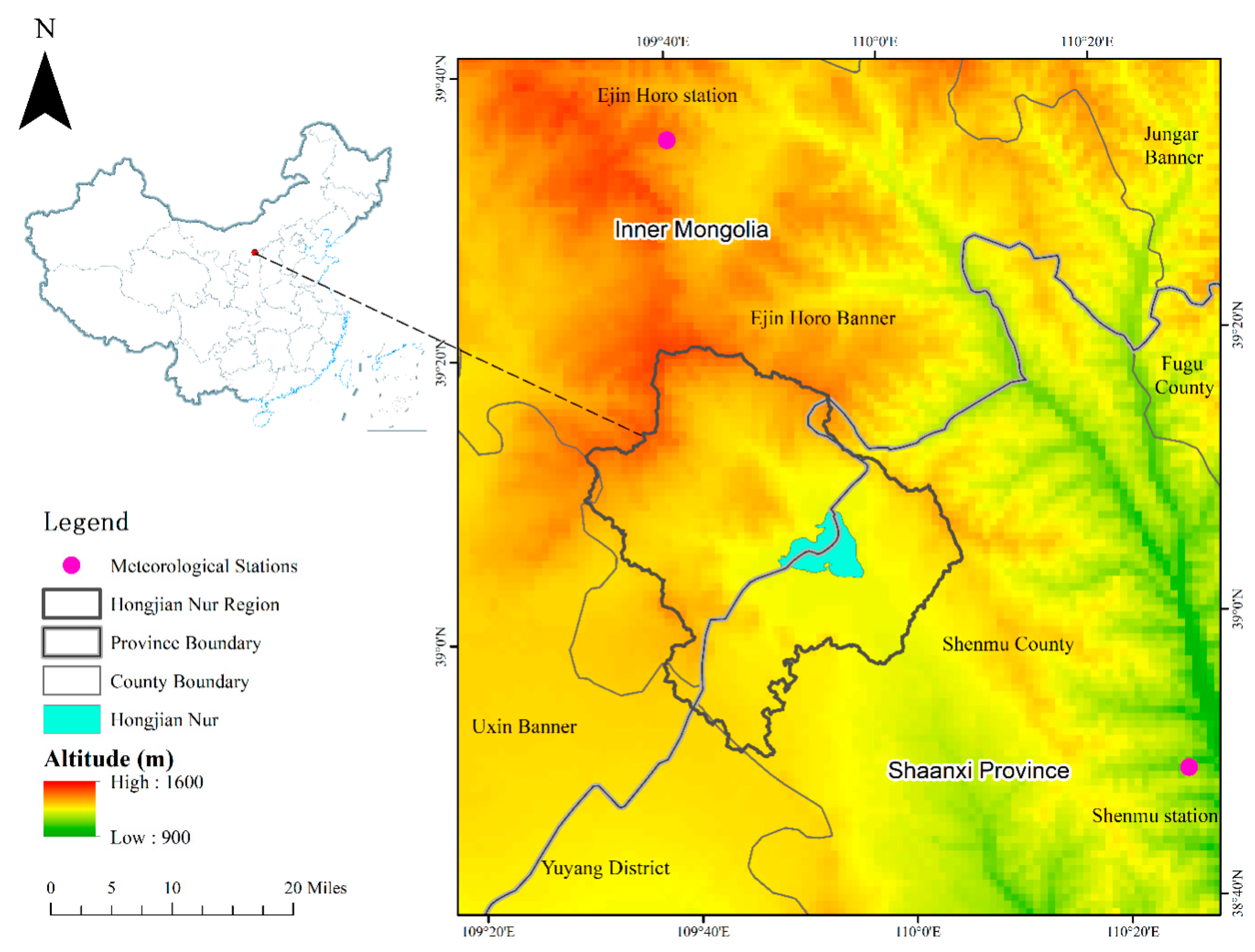
Hongjian Nur (HJN) Lake, which is known as the ‘Pearl of the Desert’, is the largest and youngest natural inland freshwater desert lake in China [11]. It is located at the border of Shenmu County in Shanxi Province and Ejin Horo Banner in the Inner Mongolia Autonomous Region. Further, it is adjacent to the Mu Us Desert. The unique geographical environment and climatic conditions of HJN Lake form an important habitat for aquatic birds and fishes. At present, HJN Lake has the largest breeding population of relict gulls in the world. HJN Lake is an oasis in the desert and has characteristic topography. It is located in desert foothills and plays an important role in water conservation, windbreak functions, sand fixation, and biodiversity maintenance. The ecological status of HJN Lake is quite important because it is a good indicator of environmental changes and climate conditions in local and riparian areas [12,13]. HJN Lake provides safe agricultural production and domestic water for residents around the basin. In 2017, the Ministry of Environmental Protection of China approved the HJN Nature Reserve for promotion to a national nature reserve [14].
HJN is on the southern margin of the Mu Us Desert, where serious desertification and low vegetation coverage (VC) have resulted in ecological fragility in the HJN watershed. Human influence is obvious in this area. Under the influence of natural factors and human activities, the water area of HJN Lake is gradually shrinking and the ecological function of the water is being degraded [15]. The upstream dam interception leads to downstream dryness and the river connectivity is further deteriorated [
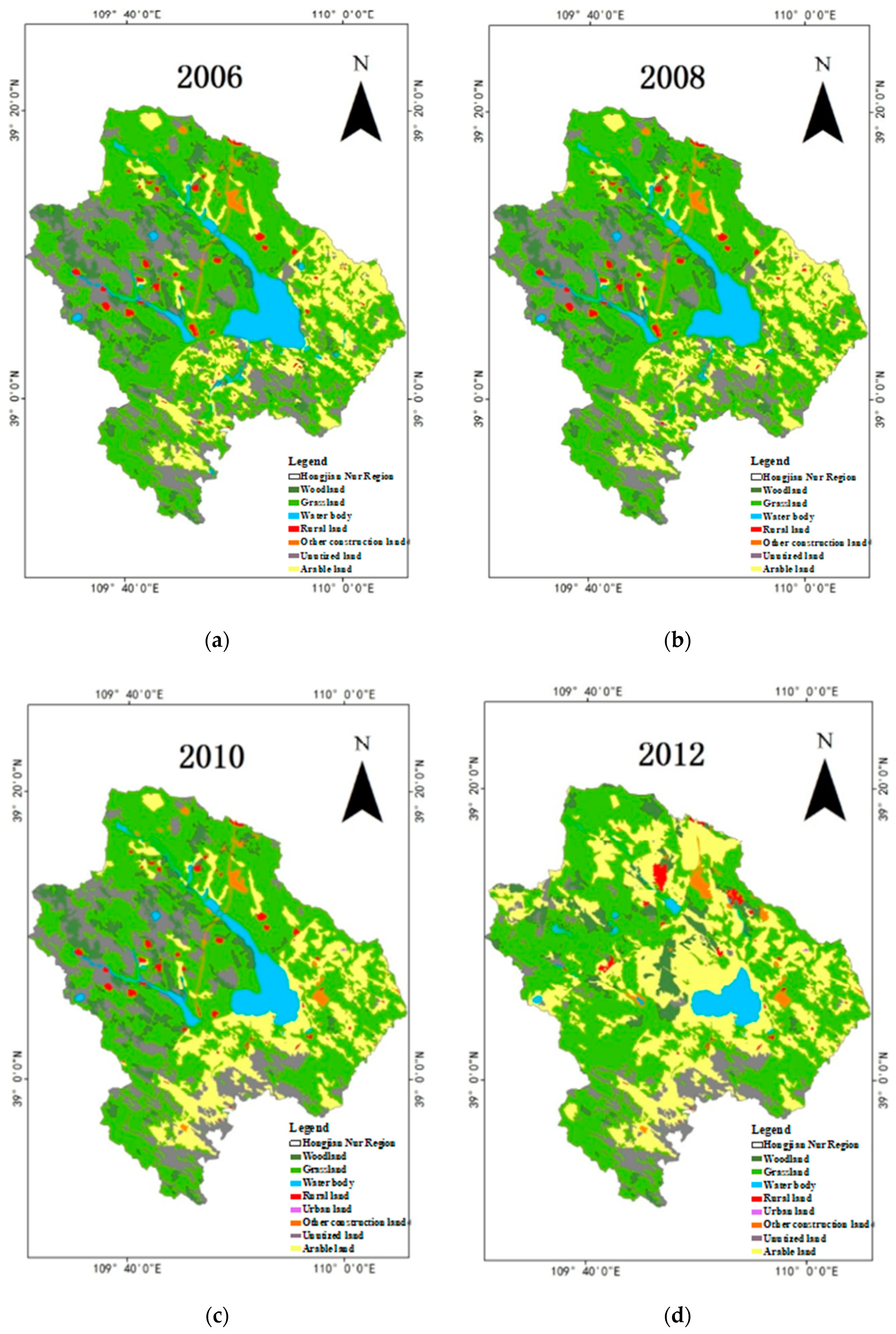
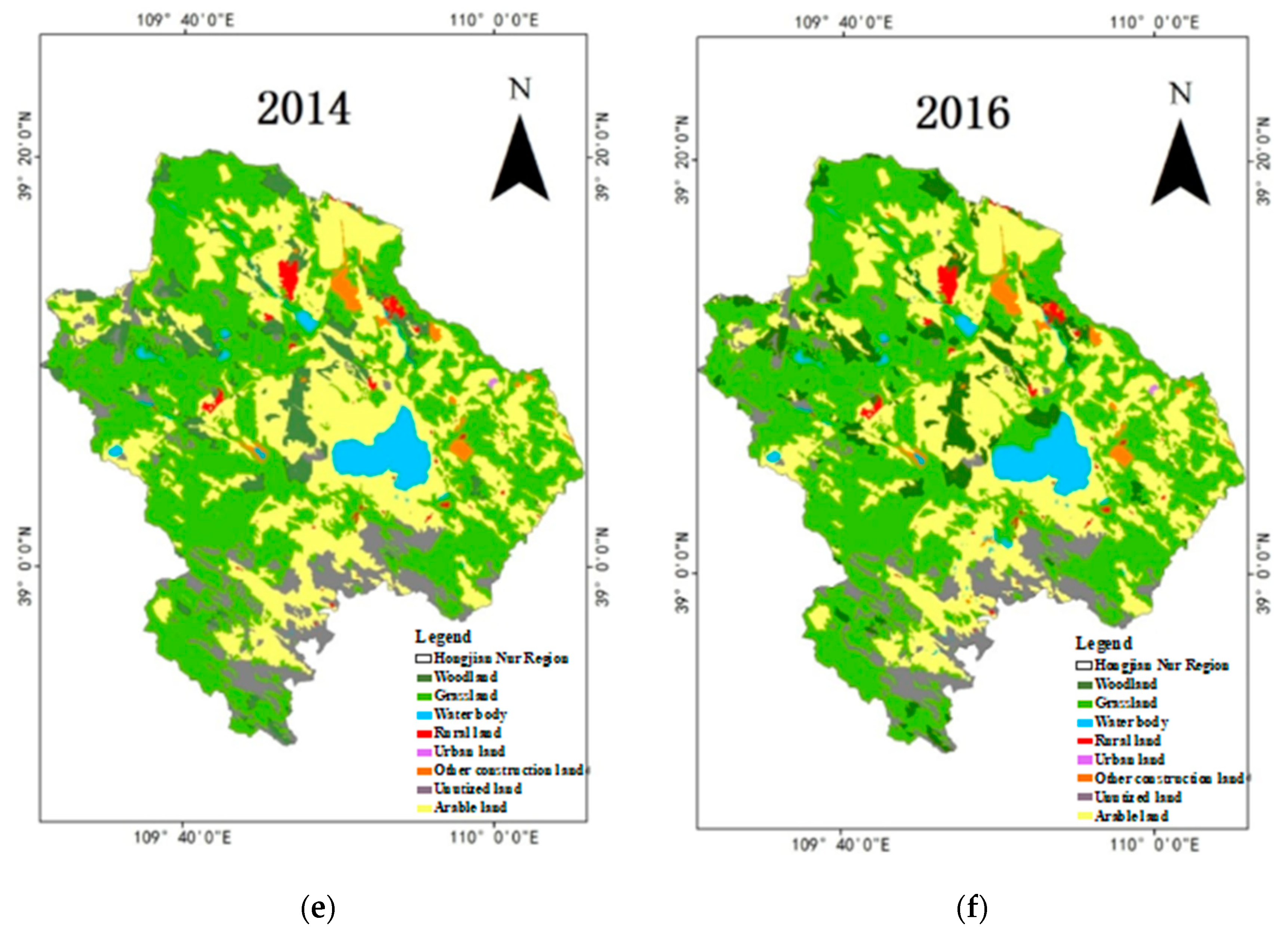
16]. The ecological environment in HJN Lake is deteriorating and the ecological security of the basin is threatened. VC and land use change are direct indicators of changes in the ecological environment and largely represent the overall state of the ecological environment [17,18]. The study of the change in VC and land use types in the HJN watershed is helpful for understanding and managing the overall ecological environment. The results of investigations of VC and land use in HJN Lake can also help simulate the dynamic change characteristics of terrestrial ecosystems [11]. They can reveal the possible factors influencing ecological environmental changes in HJN Lake, which provide reference for the protection of relict gull habitat. Furthermore, understanding the vegetation and land use conditions in HJN Lake will provide useful information and theoretical support for the HJN National Nature Reserve that is under construction.
In recent years, there has been an increasing number of studies on the ecological environment in the HJN Lake water body [19,20]. However, research on the ecological environment of the whole river basin is still insufficient. Related studies have shown that since the 1990s, the water surface area of HJN Lake has dramatically shrunk, the water level has rapidly declined, and the water quality has deteriorated [20,21,22]. The shrinkage of the water surface is the result of a combination of climate change and human impacts [23]. Under the combined effect of these two factors, the vegetation cover and land surface types around HJN Lake have changed. The changes in water area, water quality index, and surrounding vegetation of HJN Lake in the past 40 years were analyzed based on eight days of Landsat data and the normalized difference vegetation index (NDVI) from 1973 to 2013 [24]. The increase in NDVI fluctuation around the lake area indicates a trend of water retreat [
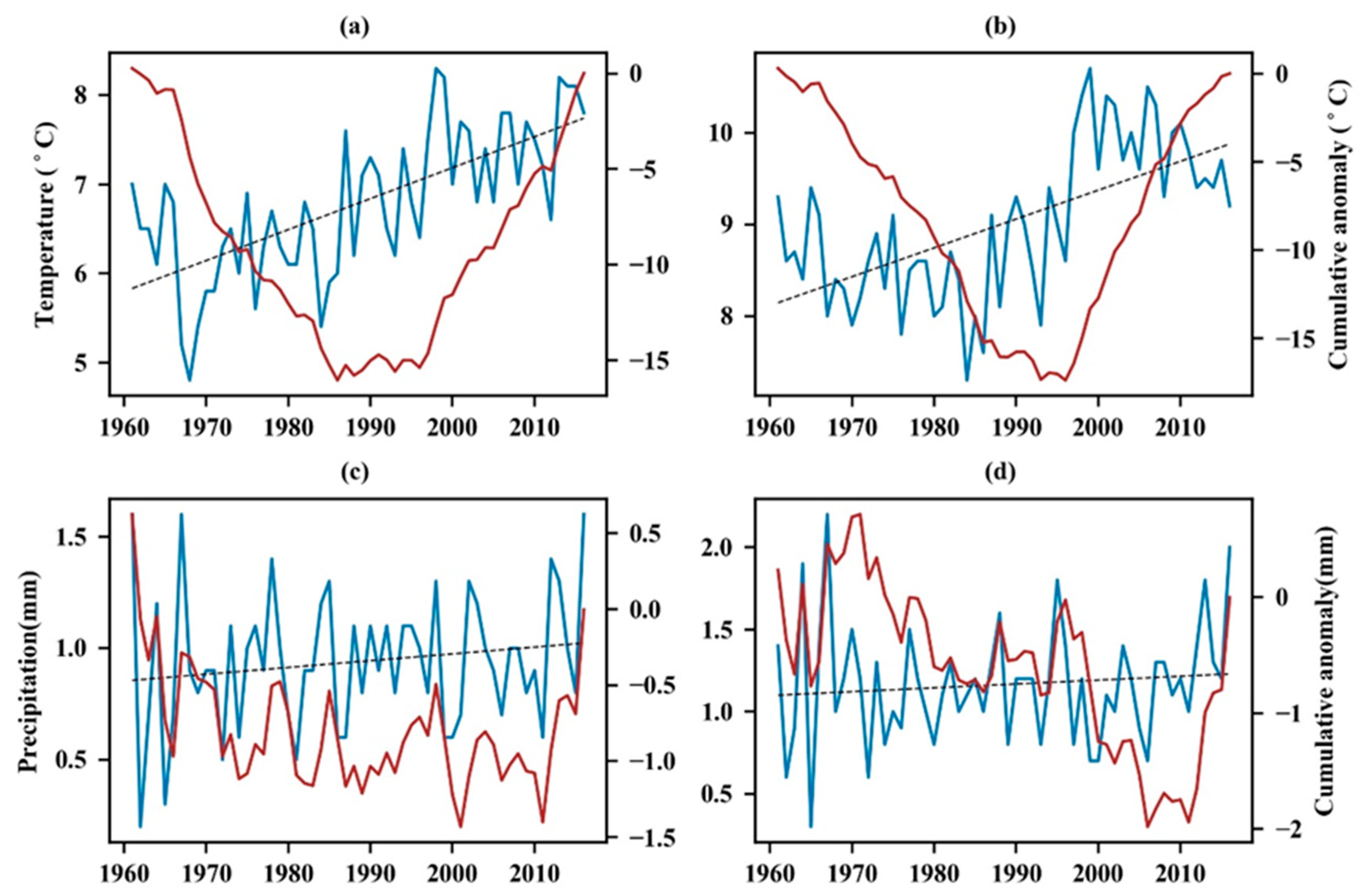
24]. Li et al. studied the effects of human activities and climate change on the vegetation cover change in the HJN region from 1982 to 2007 [19]. The results showed that the gradual increase in temperature might be the main influencing factor on the increasing trend in vegetation cover in the HJN area. Other related studies also revealed that the overall land-use change in the HJN watershed from 1989 to 2007 was characterized by a decrease in the area of lakes, other waterbodies, and sandy land, yet an increase in the area of farmland, woodland, and grassland [
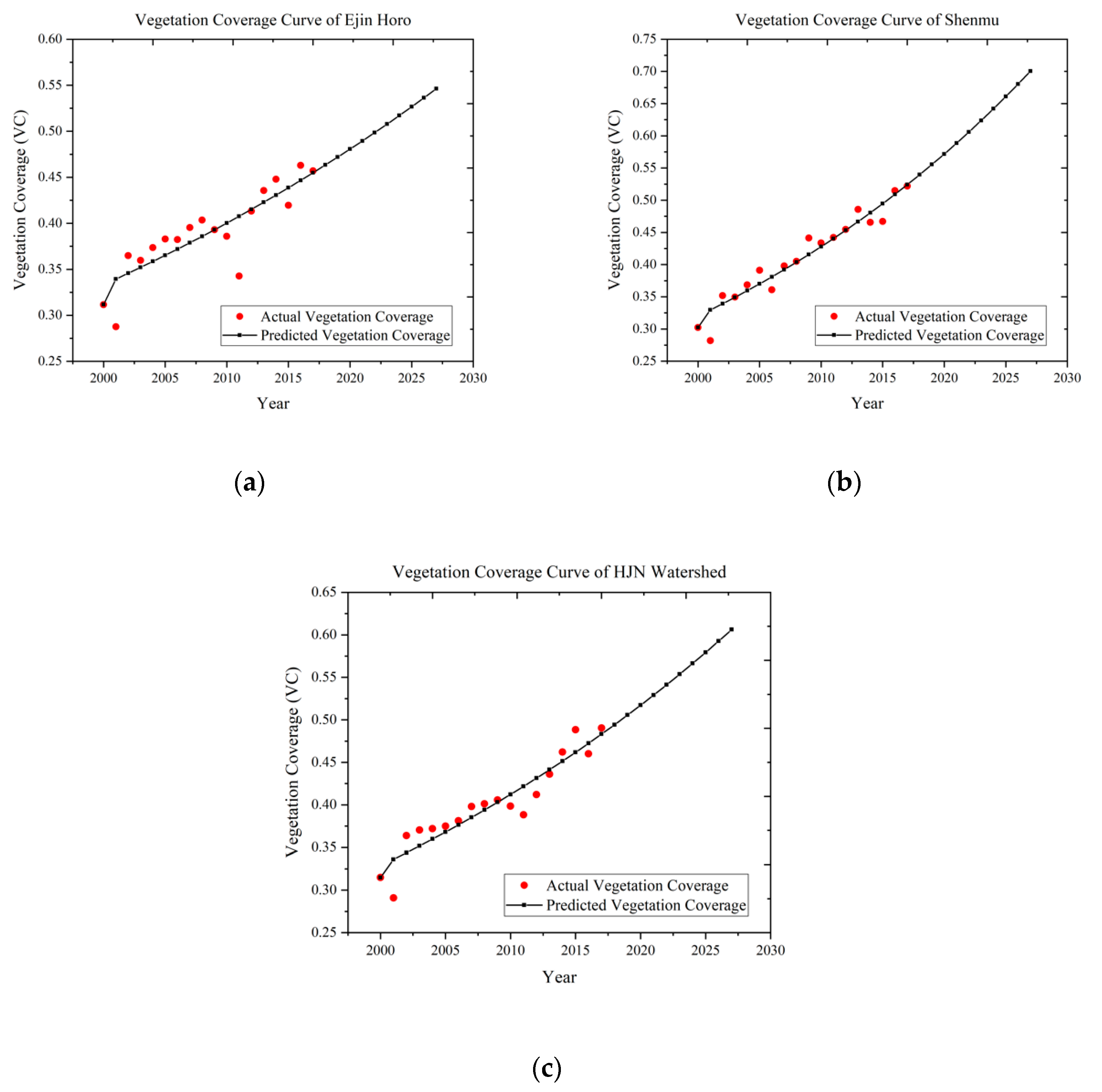
25]. Grey forecasting models, especially the first-order and single-variable grey dynamic model (GM (1,1)), are robust tools for forecasting, especially when the original sequence data are limited [26]. GM (1,1) has been successfully used for agricultural, environmental and resource predictions, proving its accuracy for modeling [27,28]. However, the GM (1, 1) model used for VC simulation and prediction is still insufficient.
The studies above have partially revealed the characteristics and trends of VC and land use change in the HJN region. The possible factors driving vegetation change in the HJN region were also discussed by previous studies [11]. However, the changes of the overall ecological environment of HJN is inadequate. This may be because the relevant research data sources are varied and the time series is short. Most of the existing studies separately analyzed VC and land use in the HJN region. Remote sensing data sources for vegetation cover and land use change studies include hyperspectral data, multispectral data, microwave data, and LiDAR data [29]. Moderate-resolution imaging spectroradiometer (MODIS) products have been widely used in regional VC and land use change investigations due to their wide coverage and high temporal resolution. Many models have been developed to detect VC and land use based on MODIS data [30]. The commonly used models include regression models, mixed pixel decomposition methods, and machine learning methods [18,31,32]. The application of the regression method as a regional empirical model to estimate VC at a large scale may cause problems because it is unable to accurately describe the complex land surface conditions [33,34,35]. However, machine learning methods are somewhat limited in practical applications due to their computational complexity [36]. The mixed pixel decomposition model is a commonly used method for calculating regional VC based on hyperspectral data. The binary pixel model is the most common model used in the linear mixed pixel decomposition method [37]. It is widely used to estimate VC due to its simplicity of application and the way it represents physical mechanisms [29]. Zribi et al. used the binary pixel model to decompose the radar ERS2/SAR (European Sensing Satellite—2/Synthetic Aperture Radar) signal and retrieved the vegetation coverage in the semiarid area [38]. Qi j et al. combined NDVI with a binary pixel model and analyzed the spatiotemporal dynamic change characteristics of vegetation coverage in the San Pedro basin in the southwestern United States [39]. Many other authors have used the binary pixel model to retrieve vegetation coverage and to explore its change trends over the years as well as the driving forces that affect these changes [40]. In addition, we aimed to describe the rapid reduction in lake area in the HJN region in recent years and identify any relevant relationships. We used GIS (geographic information science) technology to analyze the land use map overlay to obtain the land use transfer matrix and studied the mutual conversion relationships of land use. This method has been applied to the study of land use change in various regions [41,42].
In summary, it is still unclear why there is a long-time trend of comprehensive vegetation environment around the desert wetland. Thus, the main objectives of this study are as follows. (1) Herein, we try to reveal the dynamic change characteristics of the greening situation followed by vegetation restoration projects and their human and climatic factors based on both VC and land use monitoring. (2) We assume that the influence factors remain unchanged, simulating the long-time trend of the VC that will help provide reference for future desert wetland ecological environment protection. (3) We investigate the influencing factors for the greening situation around the typical desert wetland from the perspective of human and climate change. This study will help provide a scientific basis for the restoration of the ecological and economic functions of desert wetland area under vegetation restoration projects and climate change backgrounds.

2. Study Area and Data

2.1. Study Area

HJN Lake is located at 39°04′~39°08′ N and 109°50′~109°56′ E (Figure 1). In recent years, due to the dryness of the Taolimiao Alashan Nur in Ordos, Inner Mongolia, China, relict gulls have gradually chosen to move to and roost in HJN Lake. HJN Lake has become a crucial breeding and habitat for relict gulls. The HJN nature reserve is in northern China, at the southern edge of the Mu Us Sandy Land and between the Yike Zhao League of Inner Mongolia and the North Shaanxi Loess Plateau. It has the characteristics of a plateau erosive hilly landform. The HJN watershed is mainly controlled by the cold continental polar air mass and the influence of the marine hot air mass is low. The HJN watershed has continental monsoon climate characteristics because it is in the desert and in a loess boundary zone on the northwest edge of the East Asian monsoon region. This region has four typical seasons. Wind evaporation is strong in this region, which has low precipitation and rapid warming in spring. The summer is short with large temperature differences and more thunderstorms than other seasons. It is relatively cool in autumn but cold in winter, with less snow and rain than in other seasons. The HJN region has a grassland-desert transition landscape as a consequence of the low precipitation and high evaporation with sparse vegetation. Because of the specific geographical environment and climatic conditions of the HJN region, the vegetation and land use conditions are unique.

2.2. Data

2.2.1. MODIS Data

The MODIS data used in this study are derived from the Land Processes Distributed Active Archive Center (LP DAAC) managed by the NASA Earth Science Data and Information System (ESDIS) project [43]. The MOD13A2 vegetation index with 16-day 1 km SIN Grid V006 (standard resolution/globally produced) was used in this study to calculate the VC in the study area. There are two vegetation index (VI) values in these products: NDVI and the enhanced vegetation index (EVI). The quality assurance (QA) layers associated with NDVI and EVI were also provided with the products. As the HJN watershed has a relatively low VC, only the NDVI layer was used in our study. All cloud-contaminated pixels were removed based on their corresponding QA value.

2.2.2. Landsat Data

Landsat satellite data with a multispectral resolution of 30 m and a revisit period of 16 days were mainly used to detect land use/coverage change in the HJN watershed. In this investigation, Landsat TM/ETM+ images mainly from July to August during 2006–2016 were used to detect the land use types and their changes in the HJN region. The data used were primarily downloaded from the GloVis database of the USGS (United States geological survey) [44]. The downloaded data are the L1T product (Level 1T). According to the evaluation results of geometric accuracy stability, the L1T product has high geometric accuracy [45]. We used the Landsat Ecosystem Distribution Adaptive Processing System (LEDAPS) software to convert the DN value of each pixel in the image into the surface reflectance. The atmosphere correction mainly used the FLAASH Atmospheric correction of atmospheric correction module in envi5.3. We used a newly developed algorithm, F-mask, to remove clouds and shadows in the image [46]. All pixels affected by clouds and shadows were removed and only clear-sky observations were used for our study.

2.2.3. Meteorological Data

There are two meteorological stations Ejin Horo and Shenmu located around the study area. The daily climate data from the two stations was derived from National Meteorological Information Center [47]. Both stations had meteorological data from 1961 to 2016. However, data from many days were missed in November 1968. The missing data were replaced by an average value from two adjacent years to maintain the integrity of the data sequence.
All input data related information is shown in Table 1.

3. Methodology

3.1. VC Calculation

The mixed pixel decomposition model is a method for calculating VC [48]. It assumes that each pixel of a remote sensing image is composed of vegetation and soil. The value of each pixel contains information about its soil and vegetation composition, while the NDVI value of the mixed pixel is the weighted average sum of the VI (vegetation index) values based on the soil and vegetation composition of the pixel. The expression for calculating NDVI is as follows [49]:
NDVI = f v N D V I v e g + ( 1 f v ) N D V I s o i l
where is the value of the mixed pixel, N D V I v e g is the VI value of the pure vegetation pixel, N D V I s o i l is the vegetation index value of a pure soil pixel, and f v is the VC. Therefore, the VC can be obtained as follows [49]:
f v = ( N D V I N D V I s o i l ) N D V I v e g N D V I s o i l
where N D V I s o i l is approximately equal to the minimum value of a pure soil pixel (close to 0, in theory) and N D V I v e g is equal to the maximum value of a pure vegetation pixels (close to 1, in theory). N D V I s o i l and N D V I v e g will change in different times and places due to the influence of meteorological conditions, vegetation types, and their distributions. Seasonal changes and other factors may also influence N D V I s o i l and N D V I v e g .
The preprocessed NDVI data were treated as mixed pixel vegetation index values. First, the yearly NDVI values were obtained from NDVI images of the vegetation-growing season from May to October in 2000–2017 through the maximum synthesis method. The overall NDVI values in the HJN region were low. Then, to avoid overestimating the VC result, the maximum and minimum NDVI values over the whole tile covering the study area were calculated as N D V I v e g and N D V I s o i l , respectively. Finally, the yearly VC of the HJN watershed and the surrounding counties was calculated pixel by pixel with formula (2).

3.2. Land Use Analysis

Land use and cover change (LUCC) data were mainly obtained through the interpretation of remote sensing images per biennium during 2006–2016. All Landsat data were processed by radiometric correction and atmospheric correction. Interpretation keys were established by artificial methods. The land cover system of the International Geosphere—Biosphere Program (IGBP) was used in our study. Based on the actual land use/cover situation in the HJN region and the research results from landscape classification, the land use types were divided into woodland, grassland, water body, urban land, rural land, other construction land, unutilized land, and farmland. The satellite data were interpreted by a combination of manual interpretation and supervised classification methods. Too-small or surplus spots were eliminated or merged. The interpretation accuracy of Kappa index was calculated based on field observation data and interpretation results. Kappa coefficient is a multivariate statistical method to evaluate the accuracy of classification, which represents the proportion of error reduction in the evaluated classification compared with the completely random classification. The calculation formula is as follows:
^ K = N i r x i i ( x i + x + i ) N 2 ( x i + x + i )
where ^K is kappa coefficient, r is the number of rows of error matrix, x i i is the value on the value (main diagonal) of row i, x i + , and x + i are the sum of row i and column i, respectively. n is the total number of samples.
The land use interpretation results were consistent with the requirements for the analysis of land use dynamics in this study.

3.3. VC Prediction

VC was forecasted using data from the HJN watershed, Ejin Horo and Shenmu City from 2000 to 2017. VC in 2000–2027 was predicted by a grey model (GM) and a chart of the relationships between real values and predicted values were obtained. The grey model is used to predict the grey process that changes in a certain range and is related to time. Grey models are based on grey systems, which have the fuzziness of hierarchical and structural relations, the randomness of dynamic change, and the incompleteness or uncertainty of index data. This model does not require a large amount of regular sample data is easy to use and has high prediction accuracy.
GM (1, 1) model represents the first order differential equation model with one variable. The prediction principle of the GM (1, 1) model is the generation of a set of new data sequences with obvious trends accumulated from certain data sequences. The growth trend of this new data sequence is used to build the prediction model. Then, the accumulative method is used for reverse calculation to restore the original data sequence. Finally, the VC series can be forecasted.
The modeling principle of the grey model is as follows:
(1) Set the known reference data as: x ( 0 ) , then sum once to get,
x ( 1 ) = { x ( 1 ) ( 1 ) , x ( 1 ) ( 2 ) , x ( 1 ) ( 3 ) , , x ( 1 ) ( n 1 ) , x ( 1 ) ( n ) }
Among them,
x ( 1 ) ( k ) = i = 1 k x ( 0 ) ( i )   k = ( 1 , 2 , , n )
(2) Take the average sequence
z ( 1 ) ( 2 ) = 0.5 x ( 1 ) ( k ) + 0.5 x ( 1 ) ( k 1 )   k = 2 , 3 , , n
Then,
z ( 1 ) ( k ) = { z ( 1 ) ( 1 ) , z ( 1 ) ( 2 ) , z ( 1 ) ( 3 ) , , z ( 1 ) ( n ) }
(3) Modelling
The albinism equation of sequence x ( 1 ) is,
d x ( 1 ) d t + a x ( 1 ) = b
The above formula is discretized to obtain the grey differential equation of GM (1,1),
x ( 0 ) ( k ) + a z ( 1 ) ( k ) = b     k = ( 2 , 3 , , n )
(4) Solve for the equation parameters a and b
μ = ( a , b ) T , Y = { x ( 0 ) ( 1 ) , x ( 0 ) ( 2 ) , , x ( 0 ) ( n ) } T
B = [ z ( 1 ) ( 2 ) 1 z ( 1 ) ( 3 ) 1 z ( 1 ) ( 4 ) 1 z ( 1 ) ( n ) 1 ]
Using the least square method, is obtained,
J ( u ^ ) = ( Y B u ^ ) T ( Y B u ^ )
Achieve the minimum value,
u ^ = ( a , b ) T = ( B T B ) 1 B T Y
(5) Establishment of prediction formula
The prediction formula of x ( 1 ) ,
x ^ ( 1 ) ( k + 1 ) = { x ( 0 ) ( 1 ) b a } e a k + b a     k = ( 1 , 2 , , n )
The prediction sequence x ^ ( 1 ) of sequence x ( 1 ) is obtained and the prediction sequence x ^ ( 0 ) of x ( 0 ) can be obtained by reducing x ^ ( 1 ) ,
k = ( 1 ,   2 ,   ,   n ) x ^ ( 0 ) ( k + 1 ) = x ^ ( 1 ) ( k + 1 ) x ^ ( 1 ) ( k )     k = ( 1 , 2 , , n )
For the grey prediction model, the mean square deviation ratio C and the small error probability p are generally needed. The smaller the C value is the closer the p value is to 1 and the better the prediction effect of the model is. Otherwise, the worse the prediction effect is.

3.4. Statistics and Time Series Analysis

3.4.1. Zonal Statistics Method

Zonal statistics were used to analyze the general VC and land use conditions. With the zonal statistics method, a statistic is calculated for each zone defined by a zone dataset, based on values from another dataset (a value raster). A single output value is computed for every zone in the input zone dataset. Due to the regional difference of NDVI value, the mean values of VC were calculated for the study area and the surrounding districts and counties. These values are used to establish a discount chart for further analysis. The total area of each land use type in the HJN watershed was calculated to analyze the temporal and spatial land use change by the thematic map. In order to prove the accuracy of the average value of VC for more in-depth analysis, we analyzed the normality of the values in different regions for many years. A conventional descriptive statistical method was used to calculate the meteorological data for climate change analysis and to study the drivers of VC and land use variation.

3.4.2. The State Transition Matrix (STM)

STM has been widely used to analyze changes in land use types. This method was developed by Markov and was originally used to describe the probability of state transition in mathematical analysis [50]. STM not only relates the state of each land use type from the initial time to the current time but also propagates the covariance of the land use state. The land use change transition matrix can be defined as follows:
L = ( x 1 x 2 ) T
where L is the transfer matrix of land use change, with superscript T transposing each row vector to a column vector in a given time, and x 1 and x 2 are the different land use types.
In order to calculate the transfer matrix, we need to dissolve the two images rely on GIS technology. Then analyze the overlay of the two images and calculate the area of the intersection area. Finally, the transfer matrix is calculated by using the statistical tools.

3.4.3. Linear Regression

Linear regression was used to analyze the variation trends in land coverage and climate data. Linear regression is a robust model for obtaining the relationship between independent variables and dependent variables based on a least squares function. In this study, the precision of the regression or fitting was determined by the correlation coefficient and a T-test. The correlation coefficient we used was the Spearman’s rank correlation coefficient. In the correlation analysis, we used the Spearman’s rank correlation coefficient. Before calculating the coefficients, we first used SPSS 25 and Origin 2018 to verify the normality of the data, and then chose a more appropriate correlation coefficient, the Spearman’s rank correlation coefficient does not need to assume that the relationship between variables is linear or measure variables on an interval scale. It can be used for variables measured at the ordinal level. It has no strict requirements on the data and has a wider range of application [51].

4. Results

In our study, we calculated the change in vegetation coverage from 2000–2017 in HJN Lake and its surrounding areas and the change in land use from 2006 to 2016 and predicted the vegetation coverage from 2017–2027. The results showed that the vegetation coverage in HJN Lake and the surrounding areas increased significantly, and the water area of HJN Lake showed an obvious decrease.

4.1. VC of HJN Lake and the Surrounding Area

4.1.1. VC Change in the Region Surrounding HJN Lake

To understand the overall vegetation condition, the VCs of six surrounding counties were calculated and extracted. The overall VC (0.2–0.6) of the HJN watershed is lower than that of the whole calculation region (Figure 2).
The VC in the six counties around HJN Lake shows obvious spatial heterogeneity. The overall VC of Ejin Horo Banner, Uxin Banner, and Dongsheng District in Ordos city is lower than that of Shenmu County, Fugu County, and Yuyang District in Yulin city. Although they are located in the same city, Shenmu, Fugu, and Yuyang have different VC. Generally, the VC in the east is higher than that in the west in those counties. Shenmu and Fugu have higher VC than Yuyang. The eastern and northern counties as well as most parts of Fugu County have significantly higher VC than the other counties. In Yuyang County, the VC is higher only in the southeastern hilly area. The VC of Ejin Horo Banner, Dongsheng District and Wushen Banner in Ordos City is also uneven. The VC of Ejin Horo Banner is the highest, followed by that of Dongsheng district, and Wushen Banner has the lowest VC of the three.
According to the statistical analysis of the average vegetation coverage of Shenmu and Ejin Horo, the two groups of data conform to a normal distribution; the distributions are shown in the Figure 3.
From 2000 to 2017, the VC in the six county-level administrative divisions significantly changed. The overall VC in the whole region increased and the growth trend was obvious. The VC significantly increased in Shenmu and Ejin Horo Banner, which are surrounded by the HJN watershed (Figure 4). The VC in Dongsheng, Wushen and Yuyang also showed an increasing trend, but the change was not as obvious as that in the first two areas.
From 2000 to 2017, the average VC in Shenmu and Ejin Horo increased significantly increased. The VC in Shenmu County increased from 0.28 in 2001 to 0.52 in 2017. The VC in Ejin Horo Banner increased from 0.29 in 2001 to 0.46 in 2017. The average VC of the two regions was taken as the input data and the VC trend was analyzed by the linear trend analysis method. The linear fitting equation was y = 0.0124x + 0.295, R2 = 0.9403, which showed that the VC of Shenmu County increased by an average of 0.0124 per year with a significant linear growth trend. The trend fitting equation for Ejin Horo Banner was y = 0.0075x + 0.3182, R2 = 0.7328. The VC of Ejin Horo Banner increased by an average of 0.0075 per year, and the linear growth trend was remarkable.
From 2000 to 2008, the average VC of Ejin Horo Banner and Shenmu County was similar and the average VC in Ejin Horo Banner was slightly higher than that in Shenmu County. The VC of the two regions continued to increase after 2008. However, after 2009, the VC of the two regions showed obvious differentiation characteristics. The average VC increase rate of Shenmu County was obviously higher than that of Ejin Horo Banner. In Shenmu County, the VC maintained a significant increasing trend from 0.44 to 0.52 during 2009–2017. The VC of Ejin Horo Banner fluctuated after 2009, showing a trend of decreasing first and then rising during 2009–2017. The VC value reached the lowest level of 0.34 in 2011 and rose to 0.46 in 2017.

4.1.2. VC Change in HJN Watershed

The VC values in the HJN watershed from 2000 to 2017 were extracted as shown below (Figure 5).
The differentiation features of VC in the HJN watershed are not obvious. From 2000 to 2017, the VC in the HJN watershed obviously increased. In 2000, the area of HJN Lake was the largest, but the VC of the watershed was the lowest. The area of HJN Lake showed a decreasing trend from 2000 to 2006, but the VC gradually increased. The area of HJN Lake decreased significantly in 2007 and 2010, but the VC of the whole watershed maintained an increasing trend during 2007–2017. The average VC reached a maximum in 2017, with values in most parts of the whole study area reaching 0.5–0.8.
From 2000 to 2017, the average VC of the whole watershed showed a gradual increasing trend over 18 years (Figure 6). The lowest VC value was 0.29 in 2001 and then the value increased to a maximum value of 0.49 in 2017. Linear trend analysis was used to fit the change trend of VC in the HJN watershed. The linear fitting equation was y = 2.55E-5x + −62.20 with an R2 of 0.87. This indicates that the average VC of the HJN watershed increased by 2.55E-5 per year on average, which means that the vegetation condition in this area has continued to improve in recent years.

4.1.3. VC Prediction in the HJN Watershed and the Surrounding Regions

According to the calculated VC of HJN Lake and its surrounding areas during 2000–2017, a grey model was used to predict the VC from 2000 to 2027. The grey model can be used for short-, medium-, and long-term predictions. It also has good prediction accuracy for increase data. Figure 7 clearly shows that the predicted VC is consistent with the known VC in these areas. Therefore, the predicted value is highly credible and basically conforms to the development trend for vegetation coverage in the area.
To verify the accuracy of the predictions based on the grey model, the model was tested. A small-error probability P test and a variance ratio C test were performed on the model. As shown in Table 2, according to the existing rating scale that corresponds to the inspection results, the comprehensive inspection results are rated as good.

4.2. Land Use in the HJN Watershed

In 2006–2016, the area of farmland in the HJN watershed increased the most of all land use types, with the area increasing significantly from 227.31 km2 to 441.34 km2 in 2010 to 2012, respectively, and remaining basically unchanged in the following years (Table 3). At the same time, some of the area around HJN Lake was used as urban land and other construction land. The areas of woodland, grassland, water body, and unutilized land decreased gradually in this decade. The water body area decreased obviously from 86.82 km2 in 2006 to 45.35 km2 in 2016 and the area of unutilized land decreased by up to 111.26 km2. Rural land changed the least during this decade.
As shown in the Figure 8, there has been a remarkable change in the land use in the HJN watershed during 2010–2012. The area of farmland increased considerably, while the area of unutilized land decreased simultaneously. Part of the unutilized land was converted into grassland, and part of the grassland was converted into farmland. The water body also changed significantly from 2006 to 2016.
Table 4 shows that the total area of cropland and other construction land increased, while the total area of grassland, woodland, and water body decreased. The other land use types showed little change from 2006 to 2010. Among them, the total area of farmland increased by 25.52 km2, with a growth rate of 12.65%, which was mainly transformed from parts of the grassland and water body areas. The total area of other construction land increased to 14.04 km2. The total area of grassland decreased from 788.18 km2 to 771.37 km2. In addition, the total area of woodland and water bodies decreased by 1.61 km2 and 16.58 km2, respectively, and the reduction rate of water bodies was 19.10%. It is also shown clearly in Table 4 that the decrease in the total grassland and water body area is due to their transformation into farmland.
As shown in Table 5, the increase in total farmland and the decrease in unutilized land are the primary changes in land use types. The total area of farmland increased by 193.19 km2 and the increase rate was 84.99%. The added farmland was mainly transformed from grassland (162.85 km2). The total area of unutilized land decreased by 116.31 km2, with a decrease rate of 49.85%. The change in unutilized land and farmland was related to the transformation between these land use types and the grassland. The total grassland, woodland and water body area decreased by 38.7 km2, 13.38 km2, and 24.89 km2, respectively. The decrease rate of the water body area was 35.44% and it was mainly transformed into grassland, farmland, and woodland.
Combining the land use transition matrices for the two periods, the total area of unutilized land decreased by 111.25 km2 from 2006 to 2016, and the reduced area was mainly transformed to farmland, woodland, or grassland. The total area of farmland showed a significant increasing trend, with 218.71 km2 growth. The transformation of woodland and grassland to farmland was the main reason for the change in the total area of woodland and grassland.

4.3. Impact of Climate Change on VC and Land Use

Related studies have shown that the HJN watershed is a typical inland watershed [23]. VC is significantly correlated with precipitation and temperature [52]. VC is greatly affected by precipitation. However, VC has different responses to temperature and precipitation in different seasons [11]. In spring and winter, the VC is mainly affected by temperature and elevated temperature can promote vegetation growth. In contrast, the VC decreases with increasing precipitation in winter. The vegetation is affected mainly by precipitation in summer and autumn. An increase in temperature can also promote the growth of vegetation [53].
As shown in Figure 9a, the temperature showed an obvious increasing trend from 1961 to 2016 at both stations. The cumulative temperature anomaly showed that the temperature in the study area has been rising continuously since 1990. The precipitation trend is not obvious compared with that of temperature. Precipitation fluctuated before 2010, but the cumulative precipitation anomaly showed a slow downward trend. After 2010, although the HJN watershed also experienced a brief drought, the overall cumulative precipitation anomaly increased significantly. The increased precipitation and temperature promoted the increase in VC in the study area. VC increased significantly with increasing precipitation and temperature.
Before calculating the correlation between temperature and humidity and VC value, since the sample size is less than 1000, Shapiro Wilk is selected to test the normality first. Through the data test, we found that part of the data P value is low, the degree of conforming to normal distribution is low. Therefore, we used spearman coefficient to discuss its correlation. The normality test results of the data are as follows (Table 6).
The correlation coefficients between VC and the cumulative temperature anomaly and cumulative precipitation anomaly for the Shenmu and Ejin Horo stations are provided below.
As shown in Table 7, VC has a strong correlation with the cumulative temperature anomaly at both stations. The correlation coefficients between VC and the cumulative temperature anomaly reached 0.92 and 0.91 (significant at the 0.01 level) at the Ejin Horo site and Shenmu site, respectively. This indicates that the increase temperature plays an important role in the increase in vegetation in the study area. The precipitation increases also promote the increase in vegetation, with correlation coefficients of 0.73 (significant at the 0.05 level) and 0.43 between VC and the cumulative precipitation anomalies at both stations, respectively. As the increasing trend for precipitation is not obvious compared to the trend for temperature, the correlation coefficients between VC and the cumulative precipitation anomaly are lower than those between VC and temperature.

5. Discussion

5.1. Impact of Climate Change on VC and Land Use

The data from the Shenmu and Ejin Horo meteorological stations near the HJN watershed from 1961 to 2016 show that the temperature of the two stations had an obvious upward trend during this period. Precipitation fluctuated greatly before 2010. After 2010, the total precipitation accumulation increased significantly. The correlation coefficient of VC with temperature and precipitation at the Shenmu and Ejin Horo stations shows that the increase in temperature plays an important role in increasing vegetation coverage in the study area. The increase in precipitation also promotes the spread of vegetation. This result is consistent with the existing research [11]. Xiu et al. (2019) found that there was a positive correlation between average annual temperature and NDVI during 1982–2015 [11]. The investigation in other regions across the world also demonstrated the obvious relationship between climatic factors. The study over Heihe River Baisin in Northwest China found that the relationships between the changes of NDVI and temperature were significantly positive. In addition, the relationships between NDVI and temperature are higher than the relationships between NDVI and precipitation [54]. Vali et al. (2020) found that the temperature and precipitation are the main climatic factors along with topographic factors which significantly affect the vegetation distribution and change trend [55]. The spatiotemporal vegetation cover variations were also found associated with climate change in the Loess Plateau [56,57]. All these regions are located in arid areas and have many similarities with HJN in climatic or geographical divisions. Therefore, the consistent research results in various area over the world proved the credibility of the conclusion of association between climatic factors and VC.

5.2. Effect of Afforestation on VC in HJN Watershed

In the ‘12th Five-Year Plan of China (2011–2015)’, it was reported that the area of afforestation was the largest in the history of the HJN watershed and that afforestation projects had achieved remarkable results. The area preserved for various types of forest trees reached 3066 km2, with an increase of 266 km2 compared to that at the end of the ‘11th Five-Year Plan of China (2006–2010)’. A total of 863 km2 of afforestation and 441 km2 of greening mileage were completed [58]. Based on GIMMS AVHRR normalized difference vegetation index (NDVI) datasets, Wang et al. (2011) found that the vegetation coverage area of the four construction areas increased significantly after the start of the Shelter Forest System Program in the three north regions of China [59]. The greening projects mainly include greening in and around urban areas and industrial parks, the construction of green promenades and camphor pine stands, desertification control, and greening and beautification in key villages and towns. In the monitoring of vegetation cover change based on NDVI in Patuakhali District, it is also found that afforestation has an impact on vegetation cover area [60]. In our study, we also found that after afforestation, the increase in VC in the HJN watershed occurred in the context of increased greening in China from 2000 to 2017 [17,34]. This is consistent with a previous study showing that forest and farmland are the most important contributors to greening in China [17].

5.3. Relationship among VC, Land Use, and Lake Area

Human activities have a high impact on land use and vegetation cover dynamics and the soil erosion around the watershed will directly lead to the shrinkage of lake area [61]. Different research areas have shown that there is a very close relationship between vegetation coverage, land use, and lake area, which is reflected in the studies of Tso MorIri Lake, the Hulun Lake (HLL) in China, and Poyang Lake in China [62,63,64].
From 2000 to 2017, the VC of the HJN watershed was generally on the rise. In 2017, the VC of the HJN watershed reached its highest value. In addition, the vegetation coverage in the HJN watershed and its surrounding areas in 2017–2027 predicted by the grey prediction model shows that it will continue to increase. According to the land use data from 2006–2016, the increase in VC is due to the increasing areas of grassland, woodland, and cropland. In 2010, the lake area decreased significantly, which is the same finding as in a study of water areas from 1957 to 2015 by Wangying et al. However, VC continued to increase. Figure 8 and the two transfer matrices show that the reduction in the water body area of Shenmu County and Ejin Horo Banner has a close relationship with the increase in farmland. In the vicinity of the HJN watershed in 2010, the lake area clearly decreased, and the farmland area increased. This trend is consistent with that found in Liuying et al.’s research on the change in land use types in the HJN region [20]. After 2010, the VC continued to increase, while the area of the lake in the HJN watershed continued to decrease. On the whole, the increase in cultivated land area leads to an increase in VC, but it may accelerate the shrinking of lake areas [11]. As shown in Figure 8, the water area increased obviously, while the lake area decreased year by year. This means that upstream water storage aggravates the reduction of the HJN Lake area.

6. Conclusions

Our study has shown the overall VC has increased in both the HJN watershed and its surrounding region, and the upward trend in VC was obvious. This trend in VC is also revealed in the results predicted by the grey model. The results show that VC will continue to increase in the next decade. According to the statistical results for land use in the HJN watershed in 2006–2016, the areas of farmland and construction land increased, while the areas of unused land and water bodies significantly decreased. The total area of unutilized land decreased by 111.25 km2 and the reduction area was mainly transformed to farmland, woodland, or grassland. This indicates that afforestation and reclamation of farmland contribute more than other factors to the increase in VC in the HJN watershed. The increased precipitation and temperature are also beneficial to the increase in VC in the study area.
From 2000 to 2017, the VC of the HJN watershed showed an obvious upward trend, but the area of the lake decreased year by year. The increase in farmland near the HJN watershed may be the reason for the decrease in the lake size. The increase in farmland leads to an increase in VC, but it may also accelerate the decrease in lake area. The storage of water in the upstream dam further aggravates the reduction in lake size. Although human activity is an important contributor to greening in the HJN watershed, it has also led to the shrinking of HJN Lake. The ecological balance is broken in this watershed, which is located in an arid desert area. Therefore, the particularities of the local ecological environment in this desert area of China need to be considered in ecological engineering projects. For the HJN watershed, it is also important to maintain the lake area to protect relict gull habitat.

Author Contributions

Conceptualization, Lei Zhou; methodology, Lei Zhou and Siyu Wang; formal analysis, Lei Zhou, Siyu Wang, and Yinuo Zhu; investigation, Lei Zhou; resources, Jianhua Yang; data curation, Jianhua Yang; writing—original draft preparation, Lei Zhou; visualization, Siyu Wang and Yinuo Zhu; supervision, Mingyi Du and Jianjun Wu. All authors have read and agreed to the published version of the manuscript.

Funding

This research was funded by the [National Key Research and Development Program of China] grant number [2017YFC1502402], the [National Natural Science Foundation of China] grant number [41930650], the [General Project of Science and Technology Plan of the Beijing Education Commission] grant number [KM201810016014] and the [Beijing Advanced Innovation Center for Future Urban Design] grant number [UDC2018030611].

Acknowledgments

The authors would like to thank the reviewers of the manuscript for their helpful comments. We are also grateful to NASA Goddard Space Flight Center and the China Meteorological Data Sharing Service System for providing the MODIS and meteorological data used in our research.

Conflicts of Interest

On behalf of all authors, the corresponding author states that there is no conflict of interest.

References

  1. Cvetković, V.; Gačić, J.; Jakovljević, V. Impact of climate change on the distribution of extreme temperatures as natural disasters. Vojno Delo 2015, LXVII, 21–42. [Google Scholar] [CrossRef]
  2. Trenholm, R.; Haider, W.; Lantz, V.; Knowler, D.; Haegeli, P. Landowner preferences for wetlands conservation programs in two Southern Ontario watersheds. J. Environ. Manag. 2017, 200, 6–21. [Google Scholar] [CrossRef] [PubMed]
  3. Han, X.; Chen, X.; Feng, L. Four decades of winter wetland changes in Poyang Lake based on Landsat observations between 1973 and 2013. Remote Sens. Environ. 2015, 156, 426–437. [Google Scholar] [CrossRef]
  4. Zhang, Q.; Sun, R.; Jiang, G.; Xu, Z.; Liu, S. Carbon and energy flux from a Phragmites australis wetland in Zhangye oasis-desert area, China. Agric. Meteorol. 2016, 230–231, 45–57. [Google Scholar] [CrossRef]
  5. Smith, B.; Samuelsson, P.; Wramneby, A.; Rummukainen, M.J.T. A model of the coupled dynamics of climate, vegetation and terrestrial ecosystem biogeochemistry for regional applications. Tellus A 2011, 63, 87–106. [Google Scholar] [CrossRef]
  6. Danyar, S.; Yudong, S.; Jumakeld, M. Influence of groundwater level change on vegetation coverage and their spatial variation in arid regions. J. Geogr. Sci. 2004, 14, 323. [Google Scholar] [CrossRef]
  7. Fu, B.; Burgher, I. Riparian vegetation NDVI dynamics and its relationship with climate, surface water and groundwater. J. Arid Environ. 2015, 113, 59–68. [Google Scholar] [CrossRef]
  8. Zhu, L.; Gong, H.; Dai, Z.; Xu, T.; Su, X. An integrated assessment of the impact of precipitation and groundwater on vegetation growth in arid and semiarid areas. Environ. Earth Sci. 2015, 74, 5009–5021. [Google Scholar] [CrossRef] [Green Version]
  9. Elhag, A.M.H.; Ibrahim, I.S.; Dafalla, M.S. Vegetation Change Detection Using Higher Resolution Imagery in Arid Areas of the Northern State (Sudan); University of Khartoum: Khartoum, Sudan, 2016. [Google Scholar]
  10. Liu, B.; Tang, Z.; Dong, S.; Wang, L.; Liu, D. Vegetation recovery and groundwater pollution control of coal gangue field in a semi-arid area for a field application. Int. Biodeterior. Biodegrad. 2018, 128, 134–140. [Google Scholar] [CrossRef]
  11. Xiu, L.; Yan, C.; Li, X.; Qian, D.; Feng, K. Changes in wetlands and surrounding land cover in a desert area under the influences of human and climatic factors: A case study of the Hongjian Nur region. Ecol. Indic. 2019, 101, 261–273. [Google Scholar] [CrossRef]
  12. Qin, W.; Li, Z.; Liu, K.; Chen, Y. The new home of the relict gull-Hongjian Nur nature reserve in Shaanxi province, China. Life World 2016, 06, 84–93. [Google Scholar]
  13. Xiao, H.; Zhang, Z.; Wang, Z.; Wang, Y. Breeding population dynamic of relict gull (Larus relictus) at Hongjiannao lake of Shaanxi province. J. Shaanxi Norm. Univ. (Nat. Sci. Ed.) 2006, 34, 83–86. [Google Scholar] [CrossRef]
  14. Zhang, L. In Hongjian Nur, preparations are being made for buiding 5A scenic spot. New West 2018, 21–23. [Google Scholar]
  15. Ren, H.; Liu, A.; Tian, Q.; Ding, Y. Assessment of Fishery Environment Quality of Hongjiannao Lake. J. Hydroecol. 2012, 33, 96–99. [Google Scholar] [CrossRef]
  16. Yu, X.; Liu, X.; Wang, Y. Ecological risk assessment of heavy metals in the surface sediment of Hongjiannao Lake, Shaanxi Province, China. J. Earth Environ. 2016, 7, 173–182. [Google Scholar] [CrossRef]
  17. Chen, C.; Park, T.; Wang, X.; Piao, S.; Xu, B.; Chaturvedi, R.K.; Fuchs, R.; Brovkin, V.; Ciais, P.; Fensholt, R.; et al. China and India lead in greening of the world through land-use management. Nat. Sustain. 2019, 2, 122–129. [Google Scholar] [CrossRef]
  18. Gu, Z.; Ju, W.; Li, L.; Li, D.; Liu, Y.; Fan, W. Using vegetation indices and texture measures to estimate vegetation fractional coverage (VFC) of planted and natural forests in Nanjing city, China. Adv. Space Res. 2013, 51, 1186–1194. [Google Scholar] [CrossRef]
  19. Li, D.; He, H.; Liu, A. Impact of Human Activities and Climate Change on Vegetation around Hongjian Nur Lake in Northwestern China. J. Desert Res. 2010, 30, 831–836. [Google Scholar]
  20. Liu, Y.Y.; Yue, H.; Wang, T. Dynamic Change of Land Use/Cover and Spatio-temporal Evolution of Landscape Pattern in Hongjiannao Region During 1990–2015. Bull. Soil Water Conserv. 2017, 37, 224–230. [Google Scholar]
  21. Wang, J.; Guo, N.; Ma, C.F. The Dynamic Variation Characteristics of Gahai Lake Area Based on Eos-Modis Data. Int. Geosci. Remote Sens. 2012, 768–771. [Google Scholar] [CrossRef]
  22. Wang, X.B.; Xie, S.P.; Zhang, X.L.; Chen, C.; Guo, H.; Du, J.K.; Duan, Z. A robust Multi-Band Water Index (MBWI) for automated extraction of surface water from Landsat 8 OLI imagery. Int. J. Appl. Earth Obs. Geoinf. 2018, 68, 73–91. [Google Scholar] [CrossRef]
  23. Li, S.C.; Zhang, J. Environmental Changes Analysis of Hongjiannao Lake During Recent Fifty Years. Agric. Sci. Technol. 2009, 10, 178–183. [Google Scholar]
  24. Zhao, N.; Ma, C.; Yang, Y. Water quality variation of Lake hongjiannao and its driving force analysis from 1973 to 2013. J. Lake Sci. 2016, 28, 982–993. [Google Scholar] [CrossRef] [Green Version]
  25. Zhang, H.; Liu, P.; Li, X. Land use dynamic change of Hongjiannao watershed in northern Shaanxi province. Environ. Sci. Technol. 2011, 34, 180–183. [Google Scholar] [CrossRef]
  26. Naiming, X.; Ruizhi, W. A historic Review of Grey Forecasting Models. J. Grey Syst. 2017, 29, 1–29. [Google Scholar]
  27. Kang, M.; Kang, M.G.; Park, S.W.; Lee, J.J. Application Of Grey Model And Artificial Neural Networks To Flood Forecasting. J. Am. Water Resour. 2006, 42, 473–486. [Google Scholar]
  28. Ou, S.L. Forecasting agricultural output with an improved grey forecasting model based on the genetic algorithm. Comput. Electron. Agric. 2012, 85, 33–39. [Google Scholar] [CrossRef]
  29. Jia, K.; Yao, Y.; Wei, X.; Gao, S.; Jaing, B.; Zhao, X. A review on fractional vegetation cover estimation using remote sensing. Adv. Earth Sci. 2013, 28, 774–782. [Google Scholar] [CrossRef]
  30. Song, W.; Mu, X.; Ruan, G.; Gao, Z.; Li, L.; Yan, G. Estimating fractional vegetation cover and the vegetation index of bare soil and highly dense vegetation with a physically based method. Int. J. Appl. Earth Obs. Geoinf. 2017, 58, 168–176. [Google Scholar] [CrossRef]
  31. Duo, A.; Zhao, W.; Qu, X.; Jing, R.; Xiong, K. Spatio-temporal variation of vegetation coverage and its response to climate change in North China plain in the last 33 years. Int. J. Appl. Earth Obs. Geoinf. 2016, 53, 103–117. [Google Scholar]
  32. Han, W.; Zhao, S.; Feng, X.; Chen, L. Extraction of multilayer vegetation coverage using airborne LiDAR discrete points with intensity information in urban areas: A case study in Nanjing City, China. Int. J. Appl. Earth Obs. Geoinf. 2014, 30, 56–64. [Google Scholar] [CrossRef]
  33. Wang, G.; Wang, J.; Zou, X.; Chai, G.; Wu, M.; Wang, Z. Estimating the fractional cover of photosynthetic vegetation, non-photosynthetic vegetation and bare soil from MODIS data: Assessing the applicability of the NDVI-DFI model in the typical Xilingol grasslands. Int. J. Appl. Earth Obs. Geoinf. 2019, 76, 154–166. [Google Scholar] [CrossRef]
  34. Yao, R.; Wang, L.; Huang, X.; Chen, X.; Liu, Z. Increased spatial heterogeneity in vegetation greenness due to vegetation greening in mainland China. Ecol. Indic. 2019, 99, 240–250. [Google Scholar] [CrossRef]
  35. Gu, Z.; Duan, X.; Shi, Y.; Li, Y.; Pan, X. Spatiotemporal variation in vegetation coverage and its response to climatic factors in the Red River Basin, China. Ecol. Indic. 2018, 93, 54–64. [Google Scholar] [CrossRef]
  36. Okin, G.S.; Clarke, K.D.; Lewis, M.M. Comparison of methods for estimation of absolute vegetation and soil fractional cover using MODIS normalized BRDF-adjusted reflectance data. Remote Sens. Environ. 2013, 130, 266–279. [Google Scholar] [CrossRef] [Green Version]
  37. Jiapaer, G.; Chen, X.; Bao, A. A comparison of methods for estimating fractional vegetation cover in arid regions. Agric. For. Meteorol. 2011, 151, 1698–1710. [Google Scholar] [CrossRef]
  38. Zribi, M.; Hegarat-Mascle, S.L.; Taconet, O.; Ciarletti, V.; Vidal-Madjar, D.; Boussema, M.R. Derivation of wild vegetation cover density in semi-arid regions: ERS2/SAR evaluation. Int. J. Remote Sens. 2003, 24. [Google Scholar] [CrossRef]
  39. Qi, J.; Marsett, R.C.; Moran, M.S.; Goodrich, D.C.; Heilman, P.; Kerr, Y.H.; Dedieu, G.; Chehbouni, A.; Zhang, X.X. Spatial and temporal dynamics of vegetation in the San Pedro River basin area. Agric. For. Meteorol. 2000, 105. [Google Scholar] [CrossRef] [Green Version]
  40. Wang, J. Change characteristics and their causes of fractional vegetation coverage(FVC) in Shaanxi Province. Chin. J. Appl. Ecol. 2010, 21, 2896. [Google Scholar]
  41. Zoppi, C. Land cover changes and environmental protection: A study based on transition matrices concerning Sardinia (Italy). Land Use Policy Int. J. Cover. All Asp. Land Use 2017, 67, 126–150. [Google Scholar]
  42. Yao, L. Land Use and Cover Change during the Rapid Economic Growth Period from 1990 to 2010: A Case Study of Shanghai. Sustain. Basel 2018, 10, 426. [Google Scholar]
  43. Didan, K. MOD13A2 MODIS/Terra Vegetation Indices 16-Day L3 Global 1km SIN Grid V006; NASA EOSDIS Land Processes DAAC; USGS Earth Resources Observation and Science (EROS) Center: Sioux Falls, SD, USA, 2015. [CrossRef]
  44. The USGS Global Visualization Viewer. Available online: http://glovis.usgs.gov (accessed on 23 March 2020).
  45. Landsat 8, Level 1 Product Performance Cyclic Report–April 2017. Available online: https://earth.esa.int/documents/700255/1819745/IDEAS%2B-VEG-OQC-REP-2647-Landsat8CyclicReport-April2017/21cbffc8-f90f-451c-a90f-c91083bbd11e (accessed on 18 May 2020).
  46. Fu, Y.; Li, J.; Weng, Q.; Zheng, Q.; Li, L.; Dai, S.; Guo, B. Characterizing the spatial pattern of annual urban growth by using time series Landsat imagery. Sci. Total Environ. 2019, 666, 274–284. [Google Scholar] [CrossRef]
  47. National Meteorological Information Center. Available online: http://data.cma.cn/ (accessed on 23 March 2020).
  48. Cui, L.; Du, H.; Zhou, G.; Li, X.; Mao, F.; Xu, X.; Fan, W.; Li, Y.; Zhu, D.; Liu, T.; et al. Combination of decision tree and mixed pixel decomposition for extracting bamboo forest information in China. J. Remote Sens. 2019, 23, 166–176. [Google Scholar] [CrossRef]
  49. Gutman, G.; Ignatov, A. The derivation of the green vegetation fraction from NOAA/AVHRR data for use in numerical weather prediction models. Int. J. Remote Sens. 1998, 19, 1533–1543. [Google Scholar] [CrossRef]
  50. Nie, W.; Xu, T.; Du, Y.; Gao, F.; Xu, G. Numerical Algebra Solution: A New Algorithm for the State Transition Matrix. Adv. Space Res. 2017, 60, 2620–2629. [Google Scholar] [CrossRef]
  51. Hauke, J.; Kossowski, T. Comparison of values of pearson’s and spearman’s correlation coefficients on the same sets of data. Quaestiones Geographicae 2011, 30, 87–93. [Google Scholar] [CrossRef] [Green Version]
  52. He, Z.; Du, J.; Chen, L.; Zhu, X.; Lin, P.; Zhao, M.; Fang, S. Impacts of recent climate extremes on spring phenology in arid-mountain ecosystems in China. Agric. Meteorol. 2018, 260–261, 31–40. [Google Scholar] [CrossRef]
  53. Feng, Y. Vegetation Coverage Change in Mu Us Sandy Land and Its Response to Climate Change. Master’s Thesis, Beijing Forestry University, Beijing, China, 2015. [Google Scholar]
  54. Shen, Q.; Gao, G.; Lü, Y.; Wang, S.; Jiang, X.; Fu, B. River flow is critical for vegetation dynamics: Lessons from multi-scale analysis in a hyper-arid endorheic basin. Sci. Total Environ. 2017, 603/604, 290–298. [Google Scholar] [CrossRef]
  55. Vali, A.; Ranjbar, A.; Mokarram, M.; Taripanah, F. Investigating the topographic and climatic effects on vegetation using remote sensing and GIS: A case study of Kharestan region, Fars Province, Iran. Theor. Appl. Climatol. 2020, 140, 37–54. [Google Scholar] [CrossRef]
  56. Wang, T.; Kou, X.; Xiong, Y.; Mou, P.; Wu, J.; Ge, J. Temporal and spatial patterns of NDVI and their relationship to precipitation in the Loess Plateau of China. Int. J. Remote Sens. 2010, 31, 1943–1958. [Google Scholar] [CrossRef]
  57. Sun, W.; Song, X.; Mu, X.; Gao, P.; Wang, F.; Zhao, G. Spatiotemporal vegetation cover variations associated with climate change and ecological restoration in the Loess Plateau. Agric. For. Meteorol. 2015, 209–210, 87–99. [Google Scholar] [CrossRef]
  58. Su, P.; Han, Y. “Ecology +” Dressed up Beautiful Shenmu, Green Well-Being Shared by All. Available online: http://www.sxsm.com.cn/jinriyaowen/201804/t20180410_193663.html (accessed on 23 March 2020).
  59. Qiang, W.; Bo, Z.; Shengpei, D.; Yue, Z.; Zhonghua, M.; Yaning, Z. Dynamic Changes in Vegetation Coverage in the Three-North Shelter Forest Program Based on GIMMS AVHRR NDVI. Resour. Sci. 2011, 199–206. [Google Scholar]
  60. Rahman, M.M. Temporal Change Detection of Vegetation Coverage in Patuakhali Coastal Area of Bangladesh Using GIS & Remotely Sensed Data. Int. J. Geomat. Geosci. 2013, 4, 36. [Google Scholar]
  61. Lech-Hab, K.B.H.; Issa, L.K.; Raissouni, A.; Arrim, A.E.; Moussadek, R. Effects of Vegetation Cover and Land Use Changes on Soil Erosion in Kalaya Watershed (North Western Morocco). Int. J. Geosci. 2015, 6, 1353–1366. [Google Scholar] [CrossRef] [Green Version]
  62. Zhu, B.; Gu, X.; Chen, H. Analysis on Change of the Vegetation Cover in Poyang Lake Area from 1991 to 2005. Meteorol. Environ. Res. Lett. 2012, 5, 56–59. [Google Scholar]
  63. Gupta, S.K.; Shukla, D.P. Assessment of land use/land cover dynamics of Tso Moriri Lake, a Ramsar site in India. Environ. Monit. Assess. 2016, 188, 700.701–700.713. [Google Scholar] [CrossRef]
  64. Zhang, Y.; Liang, W.; Liao, Z.; Han, Z.; Xu, X.; Jiao, R.; Liu, H. Effects of climate change on lake area and vegetation cover over the past 55 years in Northeast Inner Mongolia grassland, China. Appl. Clim. 2019, 138, 13–25. [Google Scholar] [CrossRef]
Figure 1. Study area. In the figure, the elevation increases gradually from blue to brown. Blue is low and brown is high.
Ijgi 09 00364 g001
Figure 2. Changes in vegetation coverage (VC) in six counties (Shenmu, Ejin Horo Banner, Yuyang District, Wushen, Dongsheng District, and Fugu) from 2000 to 2017. (a) is the vegetation coverage in six counties in 2000; (b) is the vegetation coverage in six counties in 2005; (c) is the vegetation coverage in six counties in 2008; (d) is the vegetation coverage in six counties in 2010; (e) is the vegetation coverage in six counties in 2015; (f) is the vegetation coverage in six counties in 2017.
Ijgi 09 00364 g002aIjgi 09 00364 g002b
Figure 3. Normality of average VC in Shenmu County and Ejin Horo Banner. (a) is the normality of average VC data in Shenmu County from 2000 to 2017 and (b) is the normality of average VC data in Ejin Horo from 2000 to 2017. (c) and (d) show the normal QQ plot (Quantile-Quantile Plot) of the average VC data in Shenmu County and Ejin Horo from 2000 to 2017.
Ijgi 09 00364 g003
Figure 4. Average VC change in six counties (Shenmu, Ejin Horo Banner, Yuyang District, Wushen, Dongsheng District, and Fugu) during 2000–2017.
Ijgi 09 00364 g004
Figure 5. Spatial distribution and change in VC in the HJN watershed from 2000 to 2017. (a) is the spatial distribution and VC in the HJN watershed in 2000; (b) is the spatial distribution and VC in the HJN watershed in 2005; (c) is the spatial distribution and VC in the HJN watershed in 2008; (d) is the spatial distribution and VC in the HJN watershed in 2010; (e) is the spatial distribution and VC in the HJN watershed in 2015; (f) is the spatial distribution and VC in the HJN watershed in 2017.
Ijgi 09 00364 g005aIjgi 09 00364 g005b
Figure 6. Mean change in VC in the HJN watershed in 2000–2017. The dotted line represents the yearly mean values of VC and the red line is its linear trend fitting line.
Ijgi 09 00364 g006
Figure 7. Forecasted VC trends in the HJN watershed, Ejin Horo, and Shenmu in the next decade using a grey forecasting model (GM (1, 1) (Grey Model (1,1))). The red points represent the actual VC from 2000 to 2017 and the black line represents the predicted VC to 2027. (a) is the forecasted VC trends in the Ejin Horo; (b) is the forecasted VC trends in the Shenmu; (c) is the forecasted VC trends in the HJN watershed.
Ijgi 09 00364 g007
Figure 8. Distribution and change in land use types in the HJN watershed from 2006 to 2016. (a) is the spatial distribution and land use types in the HJN watershed in 2006; (b) is the spatial distribution and land use types in the HJN watershed in 2008; (c) is the spatial distribution and VC in the HJN watershed in 2010; (d) is the spatial distribution and land use types in the HJN watershed in 2012; (e) is the spatial distribution and land use types in the HJN watershed in 2014; (f) is the spatial distribution and land use types in the HJN watershed in 2016.
Ijgi 09 00364 g008aIjgi 09 00364 g008b
Figure 9. Temperature and precipitation trends for the Ejin Horo site and Shenmu site. (a) and (b) are the temperature trend and cumulative temperature anomaly for Ejin Horo and Shenmu, respectively. (c) and (d) are the precipitation trend and cumulative precipitation anomaly for Ejin Horo and Shenmu, respectively.
Ijgi 09 00364 g009
Table 1. Input data. MODIS: moderate-resolution imaging spectroradiometer; USGS: United States geological survey.
Data TypeData SourcePeriodTime ScaleResolution
MODIS DataLand Processes Distributed Active Archive Center
(LP DAAC)
2000–201716 days1 km
Landsat DataGlovis database of the USGS2006–201616 days30 m
Meteorological DataNational Meteorological Information Center1961–2016DailyStation
Table 2. Prediction accuracy and level and ratings of the grey model.
RegionP (Small Error Probability)C (Variance Ratio)Ratings
HJN watershed0.94440.3518Good
Ejin Horo0.88890.5115Eligible
Shenmu0.94440.2619Good
Table 3. Land use area of the HJN watershed from 2006–2016 (km2)
Year200620082010201220142016
Land Use Type
Woodland116.80117.35115.1997.6197.41101.81
Grassland788.18797.66771.38716.51710.84732.61
Water body86.8274.3270.2443.8443.8945.35
Urban land0.000.000.200.260.550.55
Rural land13.0412.3413.1311.8411.4111.41
Other construction land 19.9110.0614.0414.8815.0915.57
Unutilized land228.28229.07233.34118.55120.70117.02
Farmland201.79204.02227.31441.34444.97420.49
1 Other construction land is construction land except urban land and rural land.
Table 4. Land use area transfer matrix of the HJN watershed in 2006-2010 (km2).
Land Use TypeGrasslandFarmlandWoodlandRural LandOther Construction LandWater BodyUnutilized LandTotal in 2010
Grassland711.0235.563.501.220.003.0117.06771.37
Urban land 0.16 0.000.04 0.20
Farmland38.09162.592.501.020.0614.738.32227.31
Woodland4.170.22110.630.000.000.000.16115.19
Rural land1.370.670.0010.79 0.050.2413.13
Other construction land 13.121.010.00 9.820.000.0914.04
Water body1.210.050.000.000.0068.920.0670.24
Unutilized land29.211.520.17 0.000.10202.34233.34
Total in 2006788.18201.79116.8013.049.9186.82228.281444.82
1 Other construction land is construction land except urban land and rural land.
Table 5. Land use area transfer matrix of the HJN watershed in 2010–2016 (km2).
Land Use TypeGrasslandUrban LandFarmlandWoodlandRural LandOther Construction LandWater BodyUnutilized LandTotal in 2016
Grassland504.59 37.9953.765.963.4213.54113.35732.61
Urban land0.040.180.33 0.55
Farmland162.850.02175.5342.374.423.597.7024.02420.50
Woodland62.91 2.4614.390.860.988.7411.46101.81
Rural land7.11 1.011.171.320.020.520.2611.41
Other construction land 16.82 1.030.170.125.800.930.7015.57
Water body3.04 2.180.48 0.1738.441.0445.35
Unutilized land24.02 6.782.850.450.060.3782.50117.03
Total in 2010771.380.20227.31115.1913.1314.0470.24233.341444.83
1 Other construction land is construction land except urban land and rural land.
Table 6. Data normality test results.
PShenmuEjin Horo
VC0.837450.78743
Temperature0.641320.24194
Precipitation0.206950.08596
If P is greater than 0.05, the data is considered to be normal distribution.
Table 7. Correlation coefficients between VC and the temperature and precipitation cumulative anomalies at the Ejin Horo and Shenmu stations.
RT1P1T2P2
VC0.82 **0.78 **0.98 **0.28
** Significant at the 0.01 level. * Significant at the 0.05 level. T1 and P1 are the cumulative temperature and precipitation anomalies at the Ejin Horo site, while T2 and P2 are the cumulative temperature and precipitation anomalies at the Shenmu site, respectively.

