Graphic Simplification and Intelligent Adjustment Methods of Road Networks for Navigation with Reduced Precision

Abstract

With the rapid development of high-precision road network maps, low-precision road network maps (basic data unrelated to hardware) will need to be directly produced for traditional navigation software from high-precision maps. To do so, large amounts of vector data representing road networks must be simplified and spatial directional similarity in road networks must be maintained while reducing precision. In this study, an elite strategy genetic algorithm based on the grid model is applied to spatial directional adjustment in road networks for producing road network maps for traditional navigation. Firstly, semantic features and critical vertices are extracted from the road network with high precision. Secondly, some high-precision vertices are eliminated under constraints of the digital navigation map. During this process, the local shape maintenance of the road is considered, and the destruction of the spatial topological relationships is avoided. Thirdly, a genetic algorithm for minimizing the total changes in road azimuths at nodes of road networks is developed to maintain spatial directional relationships while reducing precision. Experimental results and visualization effects on the test data of different cities show that this method is suitable for generating road network maps for traditional navigation software from high-precision ones.

1. Introduction

Research on line simplification is valuable in the fields of computer graphics and cartography because over 80% of the elements on maps are lines [1]. The classic Douglas–Peucker (DP) algorithm [2] is essentially a process of recursively extracting valid points; the algorithm considers local as well as global features when selecting points. In the Opheim simplification algorithm [3,4], the maximum and minimum distance constraints determine the search area, thereby eliminating the intermediate original points, except the first and last points, in the search area. Visvalingam and Whyatt [5] firstly proposed an algorithm using the area as a simplified indicator. The area formed by each intermediate original point and its two adjacency efficient points is calculated. Then, the intermediate original point with the smallest effective area can be removed to ensure that the shape of the simplified line changes minimally. However, these basic algorithms do not consider the spatial topological relationship during simplification. On this basis, these algorithms have been improved. Based on the original DP algorithm, Saalfeld [6] detected and removed existing topological conflicts by dynamically updating the convex hull data structure. Like the original road, the simplified line can still maintain the correct topological relationship with the adjacent spatial objects. Pallero [7] improved the DP algorithm and proposed a robust line simplification algorithm that effectively preserves the topological relationship of the simplified polyline and is more efficient than the original DP algorithm. Tienaah et al. [8] developed a contextual model based on the DP algorithm. This model incrementally rewinds to the original polyline with relevant characteristic vertices to maintain a consistent simplification. Considering the spatial knowledge related to lines, Guo et al. [9] proposed a progressive line simplification algorithm to avoid the self-intersection of generalized lines. Park and Yu [10] proposed a methodology for segmenting lines and simplifying each section with a more appropriate simplification algorithm than any other analyzed algorithms, producing fewer positional errors based on angle and length.

Compared with removing a non-characteristic point or keeping a characteristic point at a time, the other simplification algorithms reduce the complexity of the line structure based on the preservation of the original line structure [11]. Such a reduction is achieved by removing some points, thereby creating the best-simplified line of the original line. The most representative is the constrained Delaunay triangle model for line simplification [12,13,14,15]. Considering the coastline shape and the constraints of specific areas, Ai et al. [16] proposed an algorithm that uses the curved structure of multi-branched trees to simplify coastline. In this manner, the original shape of the coastline was preserved and topological consistency was maintained. Ai et al. [17] simulated Perkal’s ε-circle rolling algorithm [18], and proposed the envelope structure of a line based on the Delaunay triangulation, which is used to compare different connections in the envelope region. The Li–Openshaw simplification algorithm [19] can produce line simplification results similar to manually generalized results based on the natural principle of objective generalization. In addition, the algorithm can be used in raster, vector, and raster–vector modes.

With the development of automatic vehicle driving technology and the improvement in map data collection methods, many high-precision road network maps for automatic driving are being continuously collected and applied, which has become one of the hot issues in research. However, the precision of road network maps for indispensable traditional navigation software provided to automobile manufacturers is relatively low. The longitude and latitude representing the high-precision location of a point retain map data up to the seventh place after the decimal, whereas the longitude and latitude in the map data for traditional navigation software only retains up to the fifth place after the decimal. For example, (15.1234567°, 16.1234567°) represents the location of a planar point, where 15.1234567° is the longitude, and 16.1234567° is the latitude. The value 15.1234567° is a number with seven decimal places. When reducing road data precision, (15.1234567°, 16.1234567°) must be rounded up to five decimal places, e.g., (15.12346°, 16.12346°). In actual applications, the road network maps with five-digit precision already meet the accuracy requirements of conventional navigation map data. Obtaining low-precision map data for conventional navigation maps is time consuming and expensive. Once the road network data with high-precision in a certain area are collected, it should be directly converted into road network maps with five-digit precision required by the conventional navigation software via cartographic generalization to avoid repeatedly surveying and mapping the road network data in the same area. This process of road network generalization involves the conversion of data precision in road network maps and has certain production requirements, such as the distance between vertices on roads, the direction of roads, the spatial directional relationship among roads connecting with the node, and the spatial topological relationship of the road network. Therefore, the abovementioned line simplification algorithms cannot be directly applied to this road network generalization. Few studies have focused on extracting road networks with five-digit precision from those with seven-digit precision. Therefore, a complete algorithm needs to be implemented, especially the optimal adjustment of the spatial directional relationship between roads at road network nodes.

Compared with original high-precision roads, the shape of five-digit-precision roads may change considerably when the precision representing the coordinates of a road vertex is reduced (Figure 1). For example, after the precision is directly reduced, the point A’ is located at position 3, whereas the azimuth deviation caused by position 2 is smaller. Thus, we focused on two problems: the simplification of roads, the maintenance of the spatial directional relationship between roads, and especially how to minimize the spatial directional change of roads after reducing accuracy. The effective area, vertical distance, buffer radius, etc., are common metrics in independent point algorithms [20], local processing routines [21,22,23,24], or global routines [25,26,27] for line simplification. As a classic line simplification algorithm, the Opheim algorithm can express the distance constraint between vertices in road networks. However, it does not consider other constraints such as turning angles of a road; therefore, for the road simplification, the Opheim algorithm must be improved.

When the data precision of roads is lowered from seven to five digits, the spatial directional relationship of simplified roads must be adjusted in accordance with the navigation requirements of road networks because the reduction in data precision causes changes in the spatial directional relationship among roads. The similarity evaluation method is based on the calculation of similarity among directional relationship matrices, as proposed by Goyal and Egenhofer [28]. It is based on the main direction distance calculation of the conceptual neighborhood graph, which is conducive to the evaluation of scene similarity. Considering direction relationships between two objects at different levels of detail, Goyal and Egenhofer [29] extended the model of the direction–relation matrix and studied the models of spatial directional relationship for arbitrary pairs of points in map generalization. Tang et al. [30,31] studied the measurement of graphical similarity among linear roads, and proposed a measuring model for linear spatial data similar based on the integration of the distance view and the feature set view, which are the views used for similarity cognition. With the developed theory of complex spatial scenes, other models for the description of the spatial scene and their similarity measures were proposed [32,33]. Yan et al. [34] focused on quantitative expressions of the features of spatial similarity relations in map spaces. Lewis and Egenhofer [35] developed a model for spatial scene description using sequences of detailed spatial intersections and object containment, capturing the connections between complex spatial objects. Buttenfield [36] presented an algorithm that maintains geometric and topological characteristics while progressively transmitting vector coordinates. However, these studies did not consider the precision reduction during road network simplification. Guo et al. [37] proposed an algorithm for the adjustment of the spatial direction relationship at the nodes of road networks only considering the local optimal solution. In this research, we applied an intelligent algorithm to find the global optimal solution in the process of adjusting the spatial direction relationship between roads at the nodes of the road network.

When the data precision is five digits, mathematically, all points on the road must be at the intersection of square grids with one length unit, so the grid model is used in this approach. We used both the improved Opheim algorithm and the spatial directional relationship maintenance of road networks to produce low-precision road network maps that meet the production requirements and visual effects. We especially focused on the change in road shape and the spatial directional relationship at nodes. The following contributions are provided by this work:

(1) An improved Opheim algorithm combined with the local shape maintenance of roads.

(2) In the process of both road simplification and adjustment of the spatial directional relationship, the consistency maintenance of topological relationships is considered to avoid topological errors.

(3) If a node is directly connected to any point that is not one of the other nodes, this node is called a general node (Figure 2). When road data precision is reduced, the spatial directional relationship among road segments connected at every general node is adjusted optimally; the change in the spatial directional relationship at every general node is the smallest after reducing precision.

(4) If two or more nodes are directly connected, these nodes are called special nodes (Figure 2). The genetic algorithm is applied with the elite strategy (e–GA) to the adjustment of the spatial directional relationship at special nodes, which helps to intelligently find the global optimal solution. The total variation in the spatial directions of road segments connected at a subgroup of special nodes can be as small as possible after the precision of road data in road network generalization is reduced.

The main steps of our method involve two workflows for road data handling (Figure 2). The first one is road simplification while maintaining the spatial direction relationship of the roads connected to the vertices, which includes the constraints in Section 2, the method for extracting road topographical features in Section 3 and the improved Opheim algorithm in Section 4. The second workflow is the maintenance of the spatial directional relationship of a subgroup of the road network connected with special nodes or a general node, which is described in Section 5. We analyze the results of the experiments in Section 6, and provide our conclusions in Section 7.

2. Constraints of Road Generalization for Navigation

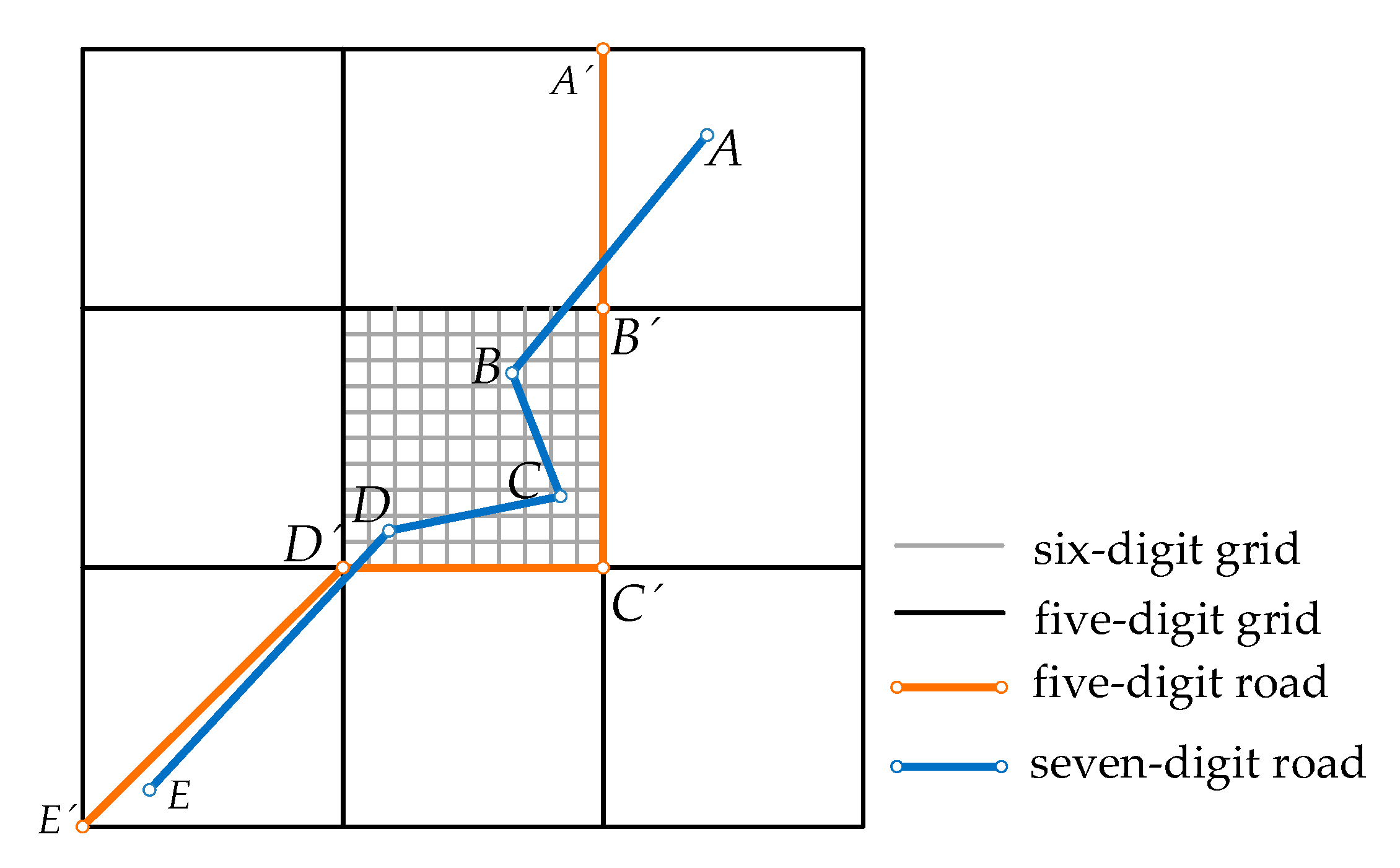
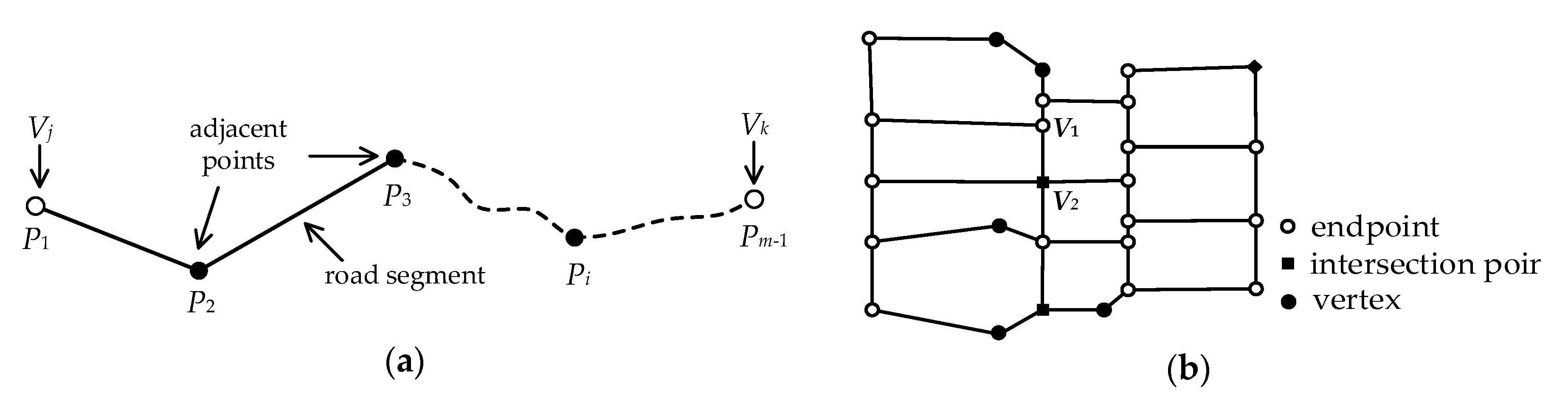
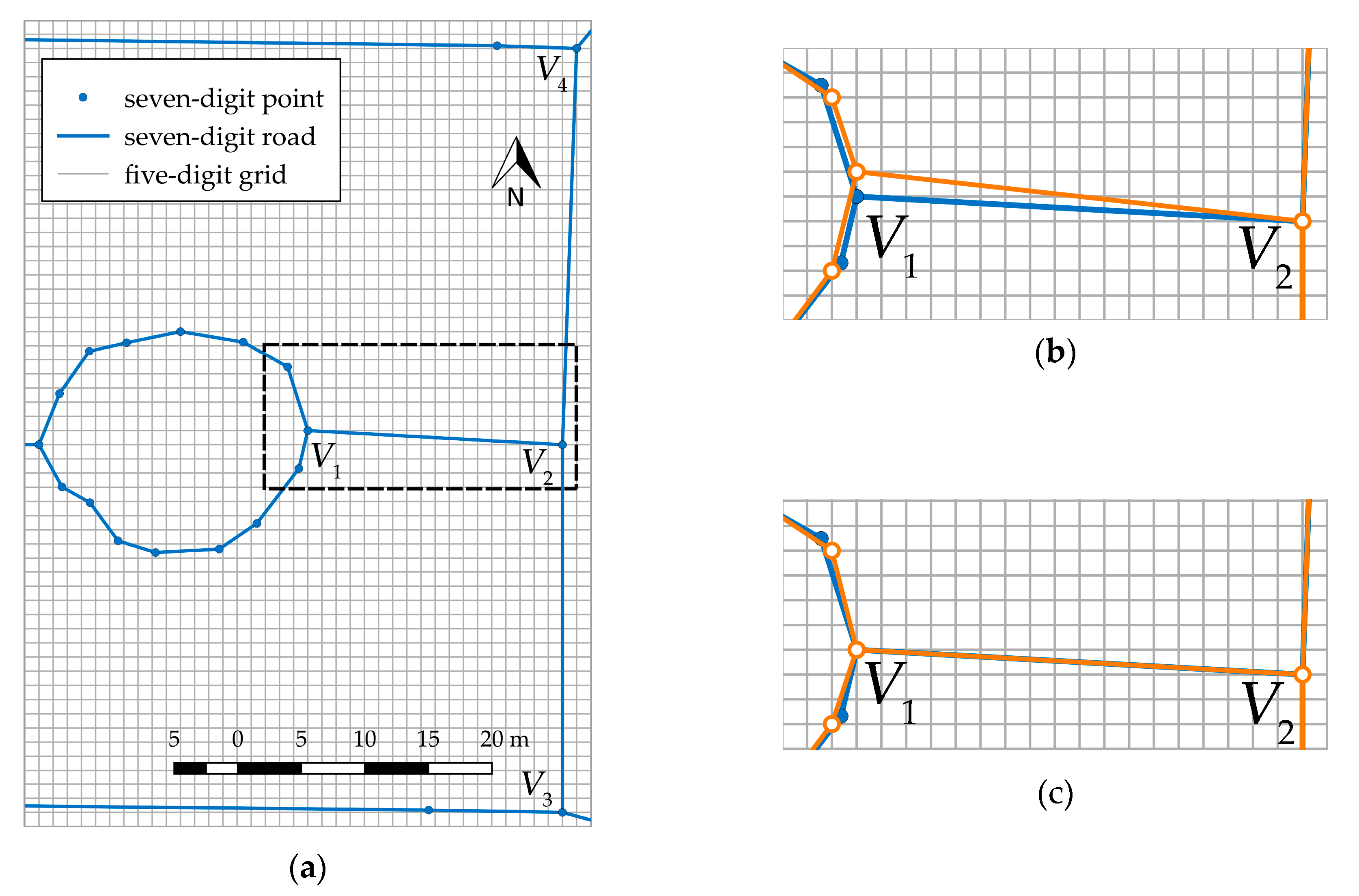
2.1. Data Model of Roads

In the road data model for navigation, a set of points {P₀, …, P_i, …, P_{m − 1}} represents a series of sequential points on the road. Nodes V_j = P₀ and V_k = P_{m − 1} represent the endpoint or the 3D virtual intersection point of the road, and point P_i (i ≠ 0, i ≠ m − 1) represents the vertex of the road, as shown in Figure 3a. 3D virtual intersection points and endpoints are distinguished in accordance with the attribute flag of points. If flag = 0, then it is the 3D virtual intersection point at which two projected roads intersect in 2D space but not in 3D space. If flag = 2, then it is the endpoint; if flag = 1, this indicates the vertex.

The road network in 2D space can be viewed as a graph structure G composed of a set of nodes V with an attribute flag and a set of edges E and is denoted as G = (V, E), as shown in Figure 3b. In the road network in this study, let an edge be the road section between two nodes and road segment be the section between two sequential points. In Figure 3a, road segment $P_1{P}_2$ is associated with node V_j, and points P₂ and P₃ are adjacent points. Therefore, three types of points exist in the road network: the intersection points, endpoints and vertices. Edges are connected at endpoints or intersection points. Thus, nodes may be endpoints or intersection points, as shown in Figure 3b. Let V_i∈V (G), and the number of edges associated with point V_i in G is called the degree of V_i [38]. In Figure 3b, the degree of node V₁ is 3, and the degree of node V₂ is 4.

2.2. Constraints on Road Generalization

The planar coordinates of points in roads can be represented by (ψ, r), where ψ is the longitude, and r is the latitude. For example, (15.1234567°, 16.1234567°) represents the location of a planar point, where 15.1234567° is the longitude and 16.1234567° is the latitude. The value 15.1234567° is a number with seven decimal places. When reducing road data precision, (15.1234567°, 16.1234567°) must be rounded up to five decimal places, e.g., (15.12346°, 16.12346°). The grid model is used to represent the different precision roads. In Figure 1, the blue line represents a road with seven-digit precision and the orange line represents the same road with five-digit precision. When a road network with seven-digit precision is generalized to five-digit precision, the four constraints on road generalization are as follows:

(1) Position precision constraint: The intersection points and endpoints cannot be eliminated, whereas the vertices may be eliminated. During local shape maintenance, the constraint of point movement is d ≤ √2δ, where d is the distance from the point with seven-digit coordinates to that with five-digit coordinates and δ is the coordinate precision defined by users.

(2) Distance constraint: The threshold of the minimum distance between two adjacent points on a road is set to ε, and ε ≤ |P_i − P_{i + 1}| ≤ k × ε (ε > √2, k > 1, which is defined by users, and P_i and P_{i + 1} are two adjacent points).

(3) Constraints for spatial directional similarity: The azimuth of the road segment is the angle between it and the northward direction. In Figure 4a, A_i is the azimuth of road segment $V_i{P}_{i+1}$ with seven-digit precision and A’_i is the azimuth of road segment $V_i{P}_{i+1}^{\prime }$ with five-digit precision. The spatial directional relationship between two sequential road segments on a road is described by the turning angle. In Figure 4b, T_i is the turning angle of two road segments at vertex P_i with seven-digit precision, and T’_i is the turning angle of the same road segment at vertex P_i with five-digit precision.

The general node V_m in the road network is unaffected by the adjustment of other nodes in the maintenance of the spatial directional relationship. In other words, no other node is connected with it (node V_m, Figure 5a). As shown in Figure 5a, all possible five-digit positions of all road segments associated with node V_m are first calculated. We can then choose the minimum sum in all possible azimuth variations. The smaller the total azimuth variation, the more similar the spatial direction. The similarity of every azimuth variation (τ) at node V_m can be calculated using Equation (1), where η₁ is the threshold of the azimuth variation of a single road segment between two adjacent points:

$$Similarity{V}_m(\tau )=\{\begin{array}{cc}\hfill 0,\hfill & \forall |A_i-A_i^{\prime }(j,k)|>{\eta }_1\mathrm{or}\mathrm{topology}\mathrm{error}\hfill \\ \hfill 1-\frac{{\displaystyle \sum _{i=0}^{M-1}|A_i-A_i^{\prime }(j,k)|}}{{\eta }_1\times M},\hfill & |A_i-A_i^{\prime }(j,k)|\le {\eta }_1\hfill \end{array}$$

(1)

where SimilarityV_m is the azimuth similarity of all road segments associated with node V_m, M is the degree of node V_m, A_i is the azimuth of road segment l_i (l_i is associated with node V_m) with seven-digit precision, A’_i is the azimuth of l_i with five-digit precision, and j and k represent the optional positions of the node and its adjacency point under five-digit precision on this road segment l_i, respectively, which range from integer 0 to 3.

If a node is connected with at least another node by a straight segment, these nodes are called special nodes (for example, Node 1~4, 6, 8~10 in Figure 6). Special nodes connected with adjacent ones must be regarded as an entirety called local subgroup G. For local subgroups G in road networks, the spatial directional similarity of every possible changed situation (τ) of the road segments connected at nodes in G can be calculated using Equation (2). The five-digit locations of the special nodes are selected when SimilarityG(τ) is the largest in all possible states.

$$SimilarityG(\tau )=\{\begin{array}{cc}\hfill 0,\hfill & \forall |B_i-B_i^{\prime }(j,k)|>{\eta }_1\mathrm{or}\mathrm{topology}\mathrm{error}\hfill \\ \hfill 1-\frac{{\displaystyle \sum _{i=0}^{N-1}|B_i-B_i^{\prime }(j,k)|}}{{\eta }_1\times N},\hfill & |B_i-B_i^{\prime }(j,k)|\le {\eta }_1\hfill \end{array}$$

(2)

where SimilarityG denotes the azimuth similarity of road segments in set L associated with special nodes in G after reducing precision. Set L stores the road segments connected to each node in G, where the data is non-duplicated. N is the number of road segments in L; B_i is the azimuth of l_i (l_i∈L) with seven-digit precision; B’_i is the azimuth of l_i with five-digit precision; and j and k represent the optional positions of the two nodes associated with l_i, ranging from integer 0 to 3.

Let P_i be the vertex on the road, and the spatial directional relationship at vertex P_i is measured by the turning angle. As shown in Figure 5b, P_{i − 1}, P_i and P_{i + 1} can be located at four optional positions when reducing precision. When the turning angle difference from seven- to five-digit precision at vertex P_i is the smallest, the similarity of spatial directional relationship at vertex P_i is the largest, as shown in Equation (3). η₂ is the threshold of turning angle variation at vertex P_i.

$$Similarity{P}_i=\{\begin{array}{cc}\hfill 0,\hfill & \forall |T_i-T_i^{\prime }(j)|>{\eta }_2\mathrm{or}\mathrm{topology}\mathrm{error}\hfill \\ \hfill 1-\frac{|T_i-T_i^{\prime }(j)|}{{\eta }_2},\hfill & |T_i-T_i^{\prime }(j)|\le {\eta }_2\hfill \end{array}$$

(3)

where SimilarityP_i indicates the spatial direction similarity of the road at vertex P_i, i (i∈{0,1, …, m − 1}) represents the ith vertex on a road, T_i is the turning angle at the ith vertex before the local shape is adjusted, T’_i is the turning angle at the ith vertex with five-digit precision after the local shape is adjusted, m is the number of vertices included on the road, and j represents one of the optional positions of vertex P’_i and is an integer from 0 to 3.

(4) Constraints for topological consistency: If vertex P_i is eliminated or moved, then the original topological relationship may be destroyed, as shown in Figure 7. In the process of vertex elimination, we can judge whether the neighborhood points are in the triangle being removed. We then know whether the elimination of point P_i destroys the topology, as shown in Figure 7a, i.e., self-intersecting polyline L₁ or polyline L₁ intersecting with polyline L₂ when removing point P_i. In the maintenance of the spatial directional relationship, as shown in Figure 7b, node V_i and any two associated road segments (e.g., l₁ and l₂) form a triangular sector S. We judge whether this adjustment leads to the loss of topological consistency by judging whether the points (e.g., point P_j) in sector S are in sector S’ formed by node V’_i and two road segments with five-digit precision after the maintenance of the spatial directional relationship. Simultaneously, the relative positions of l₁, l₂, l₃, and l₄ remain unchanged.

3. Extraction of Topographical Features on a Road Section

3.1. Extraction of 3D Terrain Feature

Slope describes the topographical feature, which is important information in navigation for a 3D road. The positive and negative signs of the slope reflect uphill and downhill, respectively. Thresholds α₁ and α₂ are given (α₁ < α₂), where α₁ represents the upper limit of the slope of the flat road, and α₂ represents the lower limit of the steep slope. Slope_i,1 is the slope of road segment $P_{i-1}{P}_i$, and Slope_i,2 is the slope of road segment $P_i{P}_{i+1}$. If and only if |Slope_i,1| ≤ α₁ and |Slope_i,2| ≤ α₁, then a partial flat road at P_i exists; otherwise, slope variation occurs.

The slope variation at vertex P_i can be expressed by ΔSlope_i, where ΔSlope_i = |Slope_i,1 − Slope_i,2|, which is related to the two road segments associated with P_i. Given threshold β when ΔSlope_i > β, the slope variation at P_i is large and P_i is defined as a critical terrain point. The six types of critical terrain points (types ①–⑥) on a road are shown in Figure 8. Axis y represents the elevation (z) of vertices on a road and axis x represents the length (x) of the road section from a vertex to the node along the road. Origin O is a node of the road. The corresponding identification methods of the critical terrain points proposed in this study are shown in Equation (4).

$$\{\begin{array}{llll}\mathrm{IF}Slop{e}_{i,1}>{\alpha }_2& \&\&& |Slop{e}_{i,2}|<{\alpha }_1& \mathrm{THEN}\mathrm{type}①\\ \mathrm{IF}Slop{e}_{i,1}<-{\alpha }_2& \&\&& |Slop{e}_{i,2}|<{\alpha }_1& \mathrm{THEN}\mathrm{type}②\\ \mathrm{IF}|Slop{e}_{i,1}|<{\alpha }_1& \&\&& Slop{e}_{i,2}>{\alpha }_2& \mathrm{THEN}\mathrm{type}③\\ \mathrm{IF}|Slop{e}_{i,1}|<{\alpha }_1& \&\&& Slop{e}_{i,2}<-{\alpha }_2& \mathrm{THEN}\mathrm{type}④\\ \mathrm{IF}Slop{e}_{i,1}>{\alpha }_2& \&\&& Slop{e}_{i,2}<-{\alpha }_2& \mathrm{THEN}\mathrm{type}⑤\\ \mathrm{IF}Slop{e}_{i,1}<-{\alpha }_2& \&\&& Slop{e}_{i,2}>{\alpha }_2& \mathrm{THEN}\mathrm{type}⑥\end{array}$$

(4)

3.2. Extraction of a Long, Straight and Flat Road

For road network maps, long, straight, and flat road sections provide important semantic information. The length threshold of a long, straight, and flat line is defined as γ, and a strip with a small width μ [23] is used to extract it from the polyline, as shown in Figure 9. Initial point P_j is at the center of the strip. The initial direction of the strip is parallel to the road segment composed of the initial point and its next point. The strip shifts over along the initial direction until the strip is just away from the polyline. Point set {P_j, P_{j + 1}, …, P_{j + m}}, which the strip has passed, forms a straight line. If the length L of the straight line is larger than γ, then the two endpoints of this road section from P_j to P_{j + m} are marked as critical topographical points for a long, straight, and flat road section. P_{j + m} is the next initial point of the remaining polyline on the road, and the same process is repeated until the strip passes the end of the polyline. Finally, all long, straight, and flat road sections are extracted.

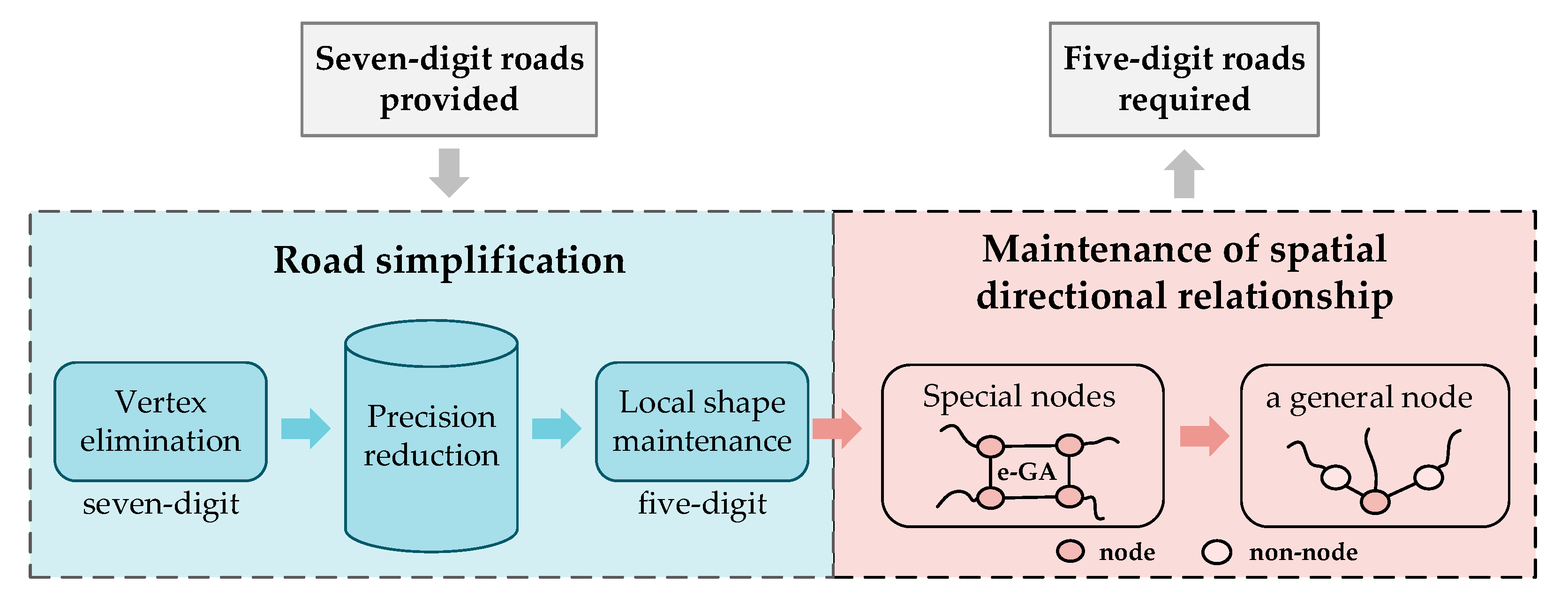
4. Road Simplification

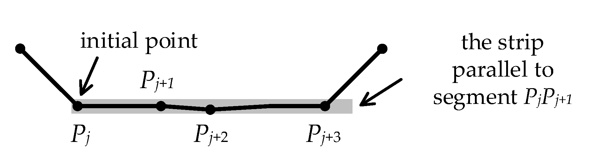
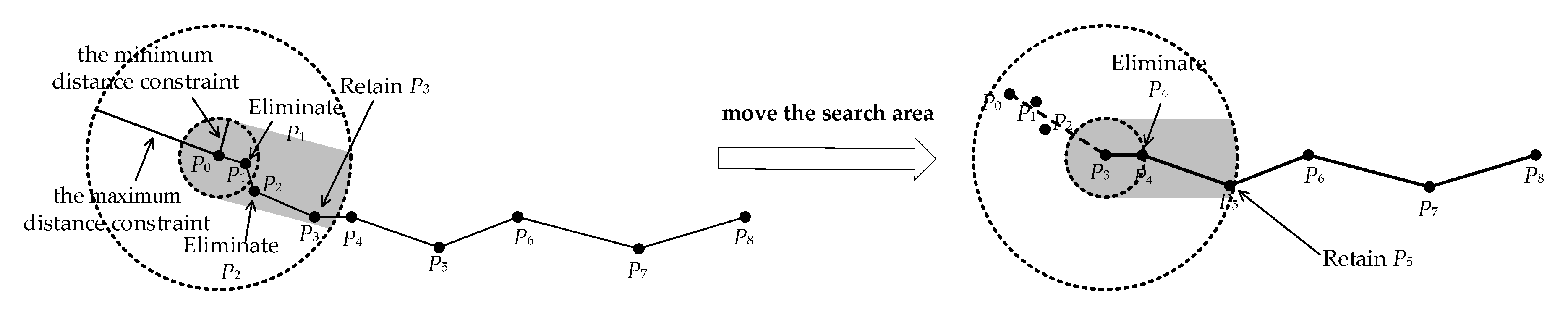
4.1. Opheim Algorithm

As shown in Figure 10, the Opheim algorithm defines the search region with the greater width μ as the strip in Figure 9, as well as a minimum and maximum distance constraint. All vertices in the search area whose radius is the minimum distance are eliminated. Except for the last vertex (P₃ in Figure 10 left) within the search area whose radius is the maximum distance, other vertices in this search area are also eliminated. Then, this undeleted vertex (P₃ in Figure 10, right) is the center of the next search area, and the vertex P₅ in Figure 10 right can be found. The search area is moved along the original line until another endpoint of this line is selected.

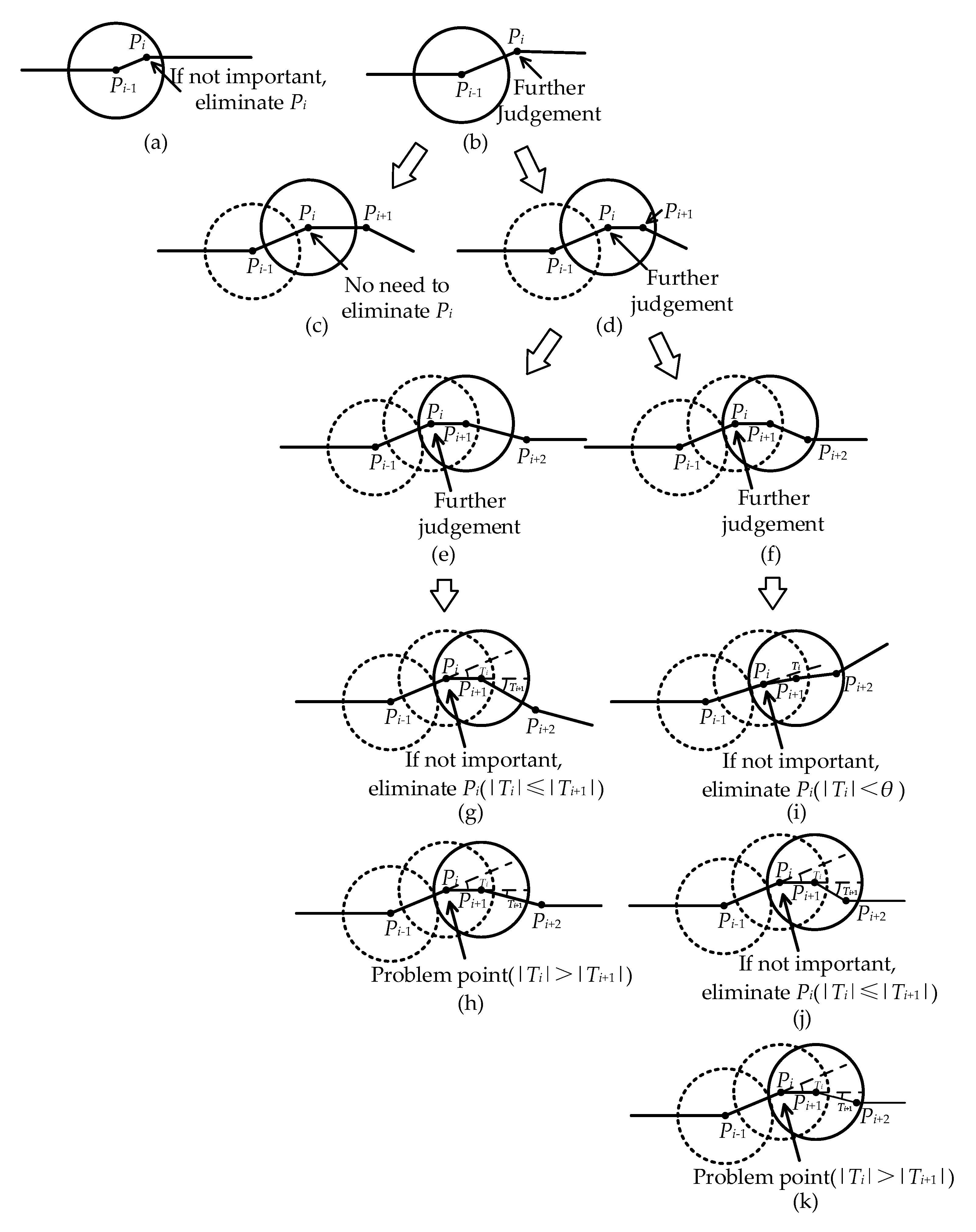
4.2. Improved Opheim Algorithm

The elimination of vertices on a long, straight, and flat road is simple and should not destroy the topological relationship. When a long, straight, and flat road section is searched, the two endpoints of this road section should not be eliminated. The vertices between the two endpoints are usually eliminated, but some vertices between these endpoints must be retained in accordance with navigational requirements; the distance between two retained sequential vertices should be larger than a threshold defined by the road network map model. In this study, the Opheim line simplification algorithm [3] was used to eliminate the vertices between two endpoints of a long, straight, and flat road section.

The elimination of vertices on curved roads is similar to that on straight roads; however, it is more complicated because all critical points and various possible situations must be considered. The minimum distance constraint threshold is ε; the search area is determined with the initial point as the center of the circle and the distance constraint threshold ε as the radius. Before vertex elimination, important critical vertices and nodes in the road network for navigation should not be eliminated. The attribute value Rank_i of every point in road topographical feature points is defined as Rank_i = 1. Other vertices’ Rank_i = 0. In the process of vertex elimination, if the elimination of vertex P_i causes topological conflicts, then Rank_i = 2. The judgment method of topological conflicts was described in Section 2.

We suppose a road R = {P₀, P₁, …, P_i, …, P_{m − 1}}, where m represents the number of vertices. Let P_i−1 be the initial point. The length of $P_{i-1}{P}_i$ is represented as D_i,1, and the length of $P_i{P}_{i+1}$ is represented as D_i,2. Each vertex P_i on the road has an attribute Remove_i, which is used to indicate whether the vertex will be eliminated. Remove_i = 0 means vertex P_i will neither be eliminated nor marked as a problem point. Remove_i = 1 means vertex P_i will be eliminated. Remove_i = 2 means vertex P_i will not be eliminated but marked as a problem point to be handled further because the elimination of vertex P_i causes a topological conflict. Given the angle threshold θ, if the absolute value of turning angle T_i at vertex P_i is smaller than the threshold θ, then vertex P_i should be eliminated. The algorithm of determining whether vertex P_i should be eliminated is illustrated in Figure 11, and the pseudocode is given as Algorithm 1.

Algorithm 1: Vertex elimination marker (R, i)

Input: A road R with m vertices (P0, …, Pi, …, Pm − 1) and a minimum distance tolerance ε

Output: point Pi with attribution value Remove /* Removei */

1. if Di,1 < ε (Figure 11a)

2.  then if Ranki = 0

3.    then call TopologicalConflict (Ranki)

4.    if Ranki = 2

5.     then Removei ← 2

6.     else Removei ← 1

7.  else (Figure 11b)

8.    if Di,2 ≥ ε (Figure 11c)

9.     then Removei ← 0

10.     else (Figure 11d)

11.      if Di + 1,2 ≥ ε (Figure 11e)

12.       then if |Ti| <= |Ti + 1| (Figure 11g)

13.         then call TopologicalConflict (Ranki)

14.         if Ranki = 2

15.           then Removei ← 2

16.           else Removei ← 1

17.     else (Figure 11f)

18.       if |Ti| < θ or |Ti| <= |Ti + 1| (Figure 11i,j)

19.        then call TopologicalConflict (Ranki)

20.        if Ranki = 2

21.         then Removei ← 2

22.         else Removei ← 1

23. end if

24. return Removei

After handling road data according to Algorithm 1, the vertices marked as problem points on this road should be handled iteratively based on the same constraints until no problem points exist on the road or problem points cannot be eliminated. Then, we handled all roads using Algorithm 1. The improved Opheim algorithm proposed in this paper emphasizes that in the one-by-one process of vertex elimination, the results of each processing step should try to destroy the spatial relationship as much as possible. If the spatial relationship is damaged, the problems must be located, and these points should be dealt with iteratively until they cannot be handled or have been handled.

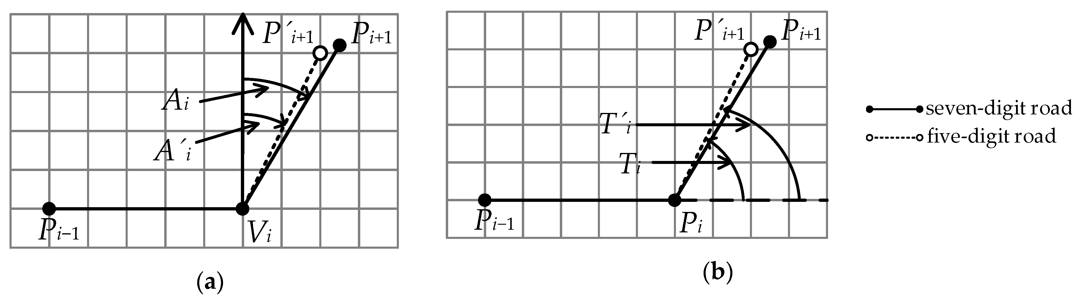
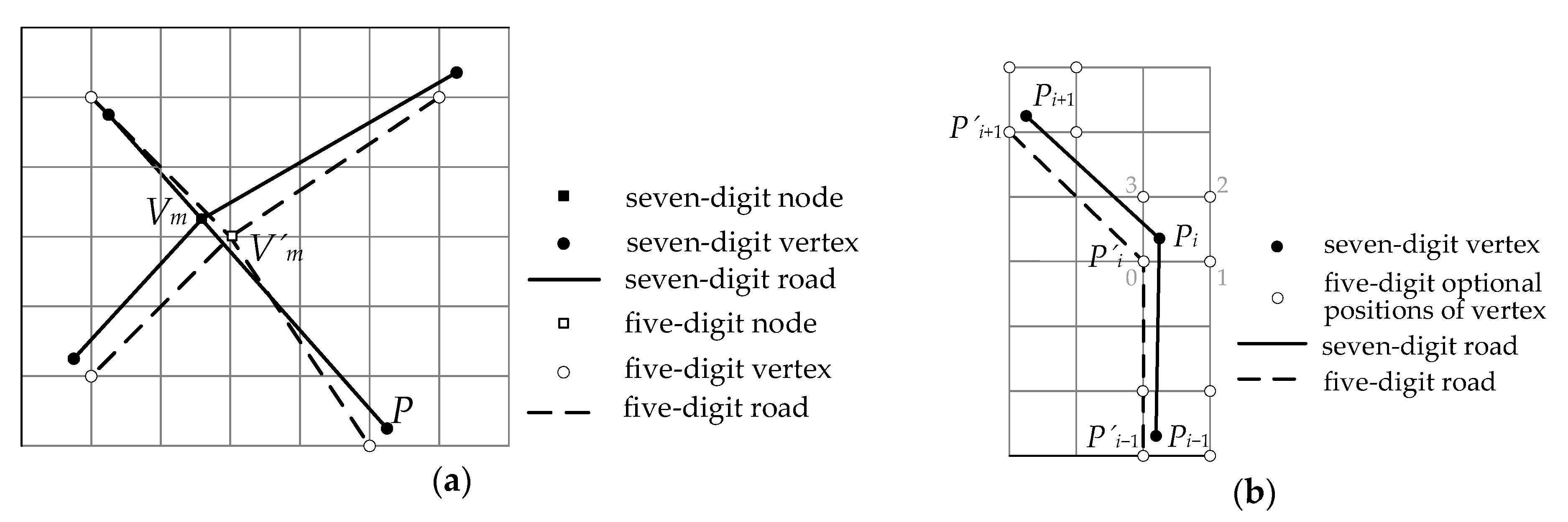
4.3. Local Shape Maintenance While Reducing Precision

As the precision of road network data is lowered, the road shape should change, as shown in Figure 1. In the grid model, each point with seven-digit precision is converted into one with five-digit precision, which has four optional positions. The change in the turning angle at point P_i is used in this study to describe the change in road shape. The spatial direction similarity SimilarityP_i at point P_i represents the local shape similarity. The angle threshold θ was given, and the absolute value of turning angle T_i at vertex P_i within the threshold θ represents a straight line. The road directions at vertex P_i have two other possibilities: if T_i > θ, then turn left; if T_i < −θ, then turn right.

Local shape maintenance should meet the following two conditions: (1) the change in direction is small and (2) the position is optimal. An optimal position means that selecting the position of its four optional positions of vertex P_i can make the local shape the most similar to the original shape, which maximizes the value of SimilarityP_i. As shown in Figure 4b, the optimal location of P_{i − 1} is supposed to have been selected. The optimal location of vertex P_i is related not only to vertex P_{i − 1} but also to vertex P_{i + 1}. The selection process of its optimal location is as follows:

(1) The impossible position of vertex P_i is removed in accordance with SimilarityP_{i − 1} under five-digit precision. Firstly, the positions with five-digit precision can satisfy the precision constraint and cannot cause the topological error. Secondly, SimilarityP_{i − 1} can be used to exclude particularly poor locations based on navigational constraints.

(2) The optimal position of vertex P_i is selected on the basis of SimilarityP_i. After precision is reduced, 16 possible connection situations theoretically exist for vertices P_i and P_{i + 1}. After eliminating impossible positions with five-digit precision, the position with the smallest SimilarityP_i in the possible positions with five-digit precision of vertex P_i is selected as optimal.

Theoretically, during the local shape maintenance of the road, when topological errors occur in all optional positions of a vertex, the position that makes the adjusted road closest to the original road shape will be selected, and topological errors will be marked in the result. After road shape maintenance, road vertices that do not satisfy the constraints under the five-digit precision should be eliminated. The detailed method was described in Section 4.1.

5. Maintenance of Spatial Directional Relationship at Nodes

5.1. Adjustment of Spatial Directional Relationship at a General Node

If a node is connected with a straight road, then this node is not a general node and is referred to as a special node here. This straight road only consists of two nodes. Thus, the general node is only adjacent to vertices. The situations of spatial directional relationship maintenance at a general node are shown in Figure 12. The function of representing the best situation in the process of spatial relationship maintenance at any general node is:

$$\max Similarity{V}_m(\tau ).$$

(5)

The algorithm is described as follows:

(1) When the precision is lowered, all possible connection situations between node V_m and its adjacent vertices are considered, and the azimuth deviations of each connection situation (τ) are calculated.

(2) The connection situations that are inconsistent with the original topological relationship and the connection situations in which the azimuth changes are greater than the given threshold η₁ are excluded, as shown in Figure 12a.

(3) The remaining connection situations are compared with one another in accordance with SimilarityV_m(τ). As depicted in Figure 12b, we choose the optimal situation under five-digit precision.

In this process, if topological errors occur in all adjustment schemes, the optimal scheme selected from them will also cause topological errors, and topological errors will be marked in the result.

5.2. Adjustment of Spatial Directional Relationship at Special Nodes

5.2.1. Difference between Two Types of Adjustments

In Figure 13a, nodes V₁, V₂, V₃, and V₄ are special nodes. On the basis of Equation (5), if the spatial directional relationship at node V₁ is adjusted first, the result of the partial region is as shown in Figure 13b. If the spatial directional relationship at V₂ is adjusted first, the result of the partial region is as shown in Figure 13c. The special nodes directly affect one another. The results of spatial directional maintenance are not only related to the threshold but also close to the processing order of special nodes. For the local subgroups of road networks directly formed by special nodes and their adjacency vertices, the results of spatial directional adjustment may not minimize the overall change in the spatial directional relationship. To solve this problem, we focused on road segments connected with special nodes in the local subgroups of road networks and constructed an intelligent algorithm to achieve the optimal combination while reducing the precision of the road network.

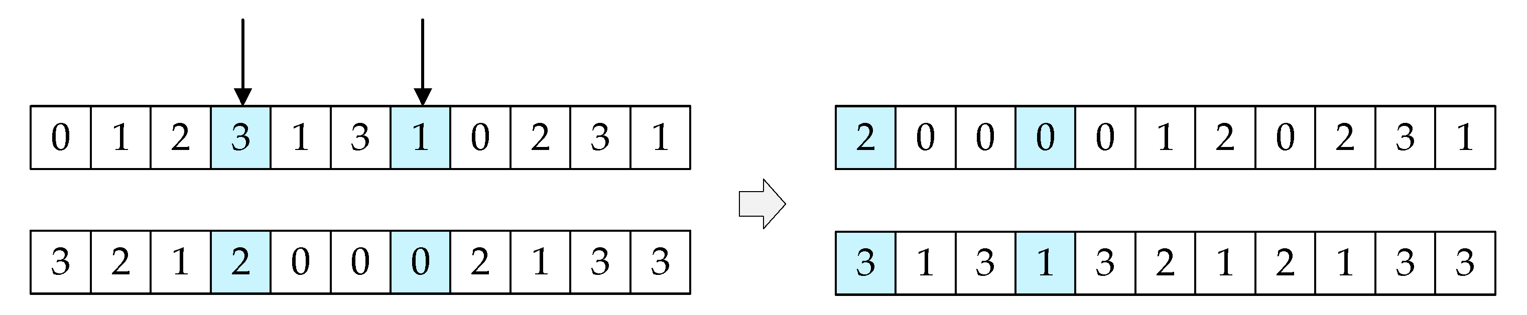
5.2.2. Elite Strategy Genetic Algorithm for Spatial Direction Adjustment

The special nodes directly connected in a road network must be organized as a community structure for spatial directional relationship maintenance called a local subgroup. Many methods for extracting community structure [39] or generalizing road networks [40] have been studied, such as a spectral algorithm for community detection based on the characteristic matrix of the network [41] and detecting communities by compressing the description of information flows on networks [42]. We used cyclic iteration in this work, and the special nodes on directly connected road networks are continuously integrated into the same local subgroup G. The adjacency vertices of road segments associated with nodes are also added to the local subgroup G as ‘virtual nodes’ to adjust them.

When the precision of road data is lowered from seven to five digits, each node or its adjacency vertex has four alternatives. 4^N optional situations exist for a subgroup of special nodes, where N is the number of nodes and their adjacency points in G. When N is relatively large, the optimal solution is impossible to find through the exhaustive method. A genetic algorithm with the elite strategy [43] was used in this study to solve the problem. Elite strategy means if the fitness of an individual in the past populations is larger than that of every individual in the current population, this string is preserved in the current generation. On this basis, we add a fixed-capacity elite retention library to retain the best individuals up to the current generation. The problem is abstracted to determine the arrangement and combination of certain items satisfying the constraints. The elite strategy can ensure that the optimal individual is not destroyed. Intelligent algorithms are widely used in map generalization [44,45,46,47]. The process for the spatial directional relationship adjustment of local subgroups of a road network based on the genetic algorithm with elite strategy (e-GA) is described as:

(1) Gene coding: Each node or its adjacency vertex in the local subgroups of road network G is abstracted as a gene, and all the genes contained constitute a chromosome or an individual, as shown in Figure 6. In the inheritance process, all individuals of each generation form a population. From seven- to five-digit precision, each node or its adjacency vertex has four optional locations. For convenience, real coding is used to directly encode gene phenotypes. The number of nodes in the local subgroups of a road network and their adjacency vertices is assumed as N, and the solution space can be modeled as a chromosome containing N genes as

$$S={\displaystyle {\prod }_{i=0}^{N-1}{C}_i},C_i=\{0,1,2,3\}$$

(6)

where S represents the solution space, i is the number of genes, and C_i is a series of alleles located on the ith gene.

(2) Adaptability evaluation. The fitness function is the basis for evaluating the quality of the results. This function is important for maintaining the spatial directional relationship. The calculation method was shown in Equation (2). The greater the fitness, the better the maintenance effect of the spatial directional relationship. The optimal solution must satisfy the maximum fitness and constraint. The constraint is

$$|A_i-A_i^{\prime }(j,k)|<{\eta }_1$$

(7)

(3) Genetic manipulation refers to selection, crossover, and variation. Holland’s roulette wheel selection [48] is the classic genetic selection operator. In this process, the better the individuals selected for mating, the greater the probability excellent genes will be inherited. For a population with number N, Group = {S₀, S₂, …, S_{N − 1} }. The fitness value of an individual is f(S_i). The probability P_i selected is

$$P_i=\frac{f(S_i)}{{\displaystyle {\sum }_{i=0}^{N-1}f(S_i)}}$$

(8)

A crossover operation is used to exchange some genes between two individuals with a certain probability to ensure the robustness of the population. The roulette algorithm was used in this study to randomly select two individuals. According to the gene size, let k₁ and k₂ be two random cross points, and k₁ and k₂ range from 0 to N − 1. Chromosomes are divided into three loci, and a sequence of gene fragments is exchanged on the basis of the crossover probability P_c (0 < P_c < 1). The crossing process of two individuals for a subgroup of special nodes is depicted in Figure 14.

The mutation operation guarantees the diversity of the population and belongs to a small-probability event. Multiple single-point mutations were used in this study to select individuals from roulette selection and crossover for random variation. The number of mutations is n (0 ≤ n ≤ N), and each time, the mutation is based on mutation probability P_m. Multiple mutations can maintain individual differences in the population and prevent premature convergence of the program.

(4) Elite strategy. Individuals with a high fitness value in the current population are kept in the elite library with number K. If their fitness value is no better than in the next generation, then individuals retained in the elite library are directly copied to the next generation and the corresponding number of the worst individuals in the next generation is replaced. The individuals in the next generation are sorted in descending order in accordance with the fitness value, and the former K individuals with large fitness values are used to update the elite retention library. When the iteration stops, the best retained individuals are approximated to the global optimal solution. Under the elite retention strategy, the genetic algorithm can converge to the global optimal solution of the problem with probability 1.

(5) Optimal solution judgment. In this study, the e-GA determines whether the cycle terminates by judging the convergence degree of the population, which is based on the change in the fitness value of the individuals retained in the elite retention library in each generation. The maximum generation is set to avoid searching for an approximate solution after the pre-accepted solution is obtained. The criteria for whether the population converges are as follows:

a. Among K best individuals in the elite retention library, the one with the smallest fitness value is better than the best individual among those in the next t generation.

b. The maximum generation is reached.

For the final K best individuals, the individuals with the smallest distance change are selected as the optimal solution from the individuals with minimal difference in fitness values. The calculation of distance change ΔD(j) is shown in Equation (9). The nodes and their adjacency vertices in the local subgroups of road network G are adjusted on the basis of the optimal scheme. In this process, the optimal scheme may cause topological errors. However, these topological errors will be marked in the result:

$$\Delta D(j)={\displaystyle \sum _{i=0}^{N-1}|D_i-D_i^{\prime }(j)|}$$

(9)

where i is the ith node or the adjacency vertex in G, j is its position, and ΔD is the sum of distance changes of the nodes and their adjacency vertices in G. D_i is the position of the ith node or the adjacency vertex in G under seven-digit precision and D’_i is the position of the ith node or the adjacency vertex in G under five-digit precision.

6. Experimental Results and Analysis

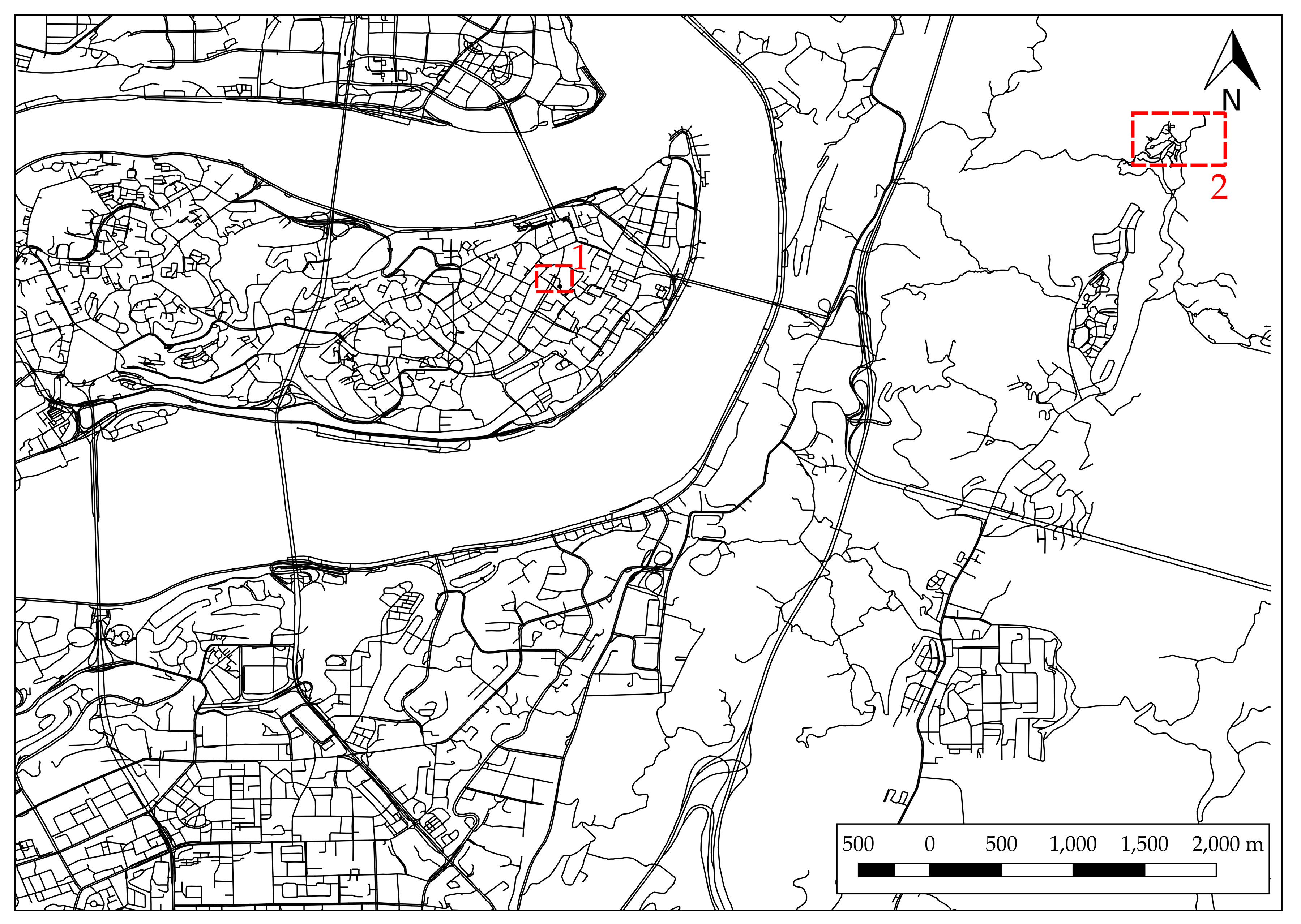
6.1. Experiments Design and Study Area

The proposed algorithm was implemented in C#, and the software developed for it can produce a road network map with five-digit precision from one with seven-digit precision. The seven-digit road network data (Advanced Driving Assistance System (ADAS) in specific formats) of a region in Chongqing, China, which was provided by NavInfo Co., Ltd. (Beijing, China), which included 53,525 roads, 106,537 endpoints, 8619 intersection points, and 118,327 vertices, were selected as experimental data. The study area is shown in Figure 15.

Given the requirements of road network data with five-digit precision, the distance constraint of vertex elimination was 2 m. The compression rate is related to the density of points in the original roads. The distance constraint ε in this experiment was set to 5 m to display the simplification details. When recognizing long straight lines, the bandwidth μ of the strip was 0.1 m, the length threshold γ of the long straight line was 100 m, and the change threshold of turning angle was 5° in the process of local shape maintenance. In the process of maintaining the spatial directional relationship of special nodes, the change threshold η₁ of the azimuth of each road segment associated with special nodes was set to 3°. The parameters and threshold setting of the genetic algorithm are shown in

Table 1. The parameters and threshold setting of the genetic algorithm.

Parameter	Crossing rate	Variability rate	Population size	Max Genetic	Number of elites
Threshold	0.8	0.1	100	1000	20

. In Figure 15, the region in box 1 is shown in Figure 16, and the region in box 2 is shown in Figure 17. These values are not fixed but are deemed relatively reasonable for this experiment.

6.2. Result Analysis

The improved Opheim algorithm proposed in this study was compared with the classical DP, Visvalingam–Whyatt (VW), and Opheim algorithms. The data compression rates of the four simplification methods were similar, facilitating comparison of the simplification effect. The vertical distance threshold was set to 0.5 m in the DP algorithm, the area threshold was set to 4 m² in the VW algorithm, and the minimum distance constraint was set to 5 m in the Opheim algorithm. The simplified results after maintenance are shown in Figure 16. From the visual effect of the simplified line, the distance among points best met the distance constraint and showed a good approximation of the original road. Compared with our algorithm, the DP algorithm produced a better compression result for straight, long, and flat road sections, and the compression effect of the curved roads was not ideal. Especially for curved roads with large bends and dense points, the distance constraint was difficult to meet.

The regions outlined by the black dotted lines in Figure 16b show the simplified version using the DP and the proposed algorithms with five-digit precision. A considerable difference was found in whether the local road shape was maintained. The results showed that the simplified result of our algorithm is was better than that of the DP algorithm.

The simplified result of the VW algorithm is shown in Figure 16c. A few points do not satisfy the distance constraint. The road shape under five-digit precision changed more compared with the original shape, as shown in the dotted box, because road shape maintenance was disregarded.

The Opheim algorithm is similar to the current algorithm, but it does not consider the changes in turning angle and road shape. As a result, the road shape considerably changed after reducing precision. The simplification result was also not as good as that of the proposed algorithm.

Figure 17 shows four simplified results for a ring road in region 2 in Figure 15. Except for the improved Opheim algorithm proposed in this study, the DP, VW, and Opheim algorithms were unable to maintain the spatial topological consistent with the original road. The topological errors are presented in the dotted box in Figure 17. The result of the improved Opheim algorithm, shown in Figure 17a, implied that eliminating point P will lose topological consistency after simplification. Accordingly, point P was preserved and marked as a problem point. Vertex elimination under high precision guarantees results without self-intersections, regardless of the morphology of the input line and the tolerance value. In contrast, the DP, VW, and Opheim algorithms eliminated important characteristic points and violated the positional precision constraint. Figure 17b–d depict that some intersection points on the road are eliminated. The improved Opheim algorithm retained the intersection points and other feature points while satisfying the distance constraint. Another advantage of the proposed method shown in Figure 17 is that it can meet the distance requirement of road data compression better than the other methods, which do not consider the distance among reserved points.

Figure 18 is a result of maintaining the spatial directional relationship of the road network associated with the special nodes in Figure 13 by using e-GA. This result of the intelligent algorithm is generally optimal. This method keeps the morphological characteristics and displacement precision of the road network. In Figure 18, the overall azimuth deviation is the smallest, and the similarity is the highest.

To better demonstrate the performance of our method, experimental results based on the data from Chengdu (61,641 roads), Guangzhou (71,326 roads), and Shanghai (43,571 roads) in China were compared and analyzed.

Table 2. The average Hausdorff distance statistics of different methods.

City	Our Algorithm (m)	Opheim Algorithm (m)	VW Algorithm (m)	DP Algorithm (m)
Chongqing	0.308	0.390	0.671	1.043
Chengdu	0.223	0.277	0.446	0.852
Guangzhou	0.246	0.296	0.571	0.784
Shanghai	0.205	0.240	0.357	0.769

presents the comparisons of the four groups of experiments. Similarly, the compression rates of these four sets of experiments were comparable. The assessment results of the modified Hausdorff distance (MHD) [49] between the original and the simplified roads are shown in Table 2, which shows a higher shape similarity degree with our proposed method than the other three methods.

Table 3. The average changes in the azimuth angle in the spatial directional relationship.

Changes in Azimuth Angle	Chongqing (°)	Chengdu (°)	Guangzhou (°)	Shanghai (°)
Without adjustment	0.527	0.342	0.392	0.321
With adjustment	0.439	0.284	0.334	0.265

shows the changes of the azimuth angles with and without adjustment of the spatial directional relationship.

Table 4. The average changes in the turning angle in the spatial directional relationship.

Changes in Turning Angle	Chongqing (°)	Chengdu (°)	Guangzhou (°)	Shanghai (°)
Without adjustment	2.707	2.338	2.345	2.402
With adjustment	1.869	1.628	1.671	1.676

describes the changes in the turning angles with and without adjustment of the spatial directional relationship. Our method was the key to extracting road network maps with five-digit precision from those with seven-digit precision.

7. Conclusions

In this study, we innovatively proposed a method that combines the improved Opheim algorithm with the intelligent maintenance of the spatial directional relationship. Based on the grid model, this new method effectively expresses the process of transforming road network maps from seven- to five-digit precision, which involves four main steps. First, the improved Opheim algorithm under seven-digit precision deletes vertices that do not meet requirements for navigation. Second, local shape maintenance under five-digit precision is used to maintain the spatial directional relationship between the road segments connecting with the vertices. Third, the spatial directional relationship at a general node is adjusted. Finally, we explained the problems caused by the method when maintaining the spatial direction relationship between roads at special nodes, and introduced the process of solving this problem with a genetic algorithm with the elite strategy in detail. To illustrate the application of our method, we examined the road network extraction in four cities, and we proved these results to be reasonable and effective. The threshold in the experiment was set on the basis of experience. The following conclusions can be drawn from the results:

(1)

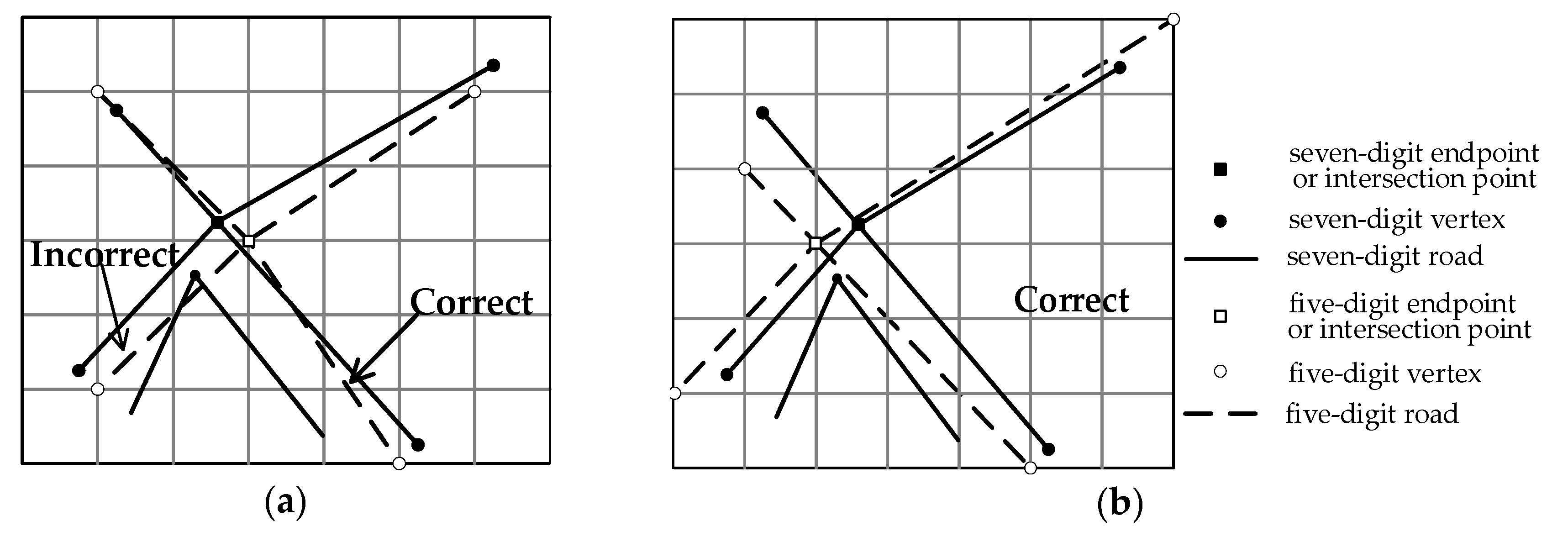
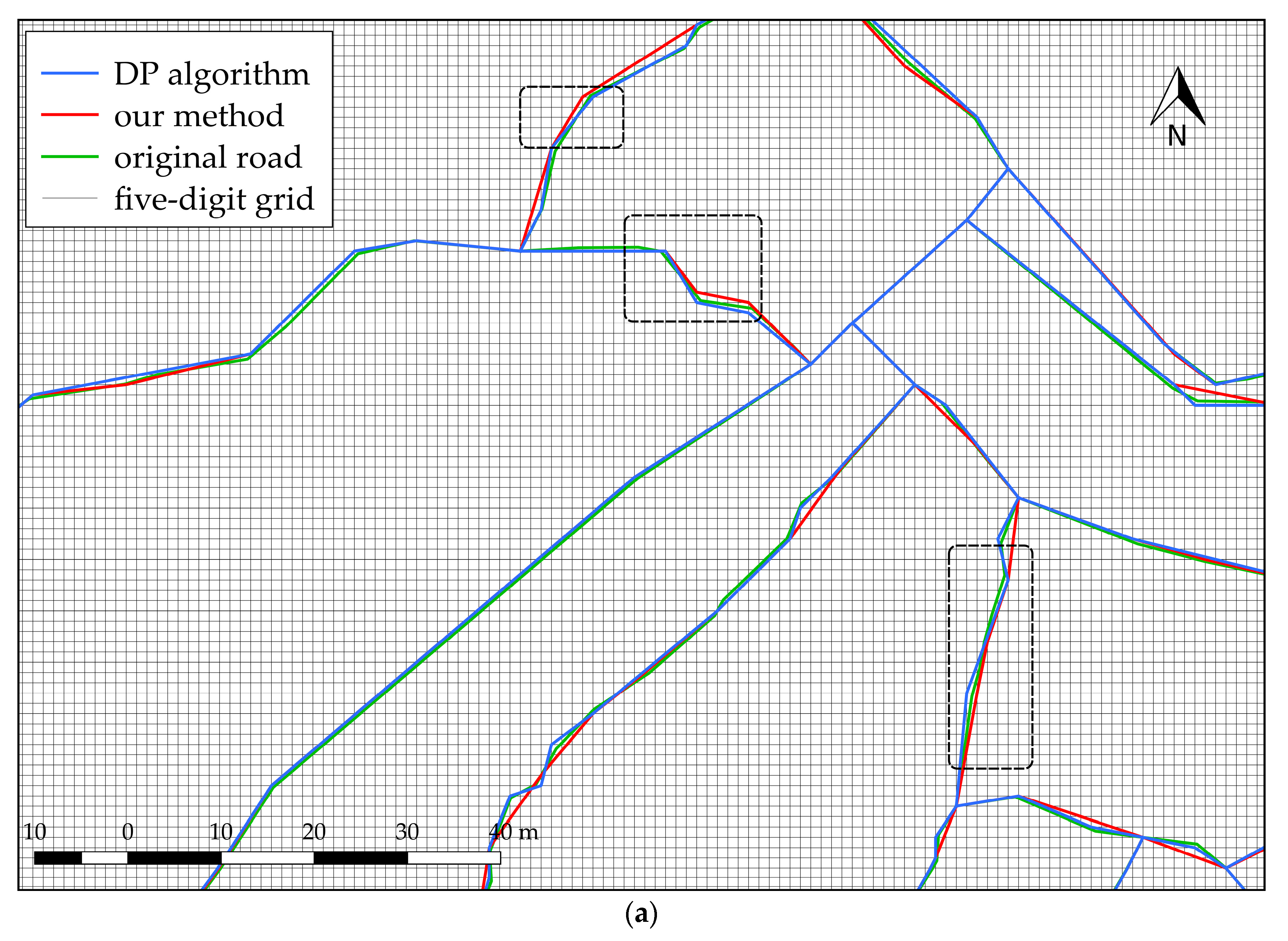
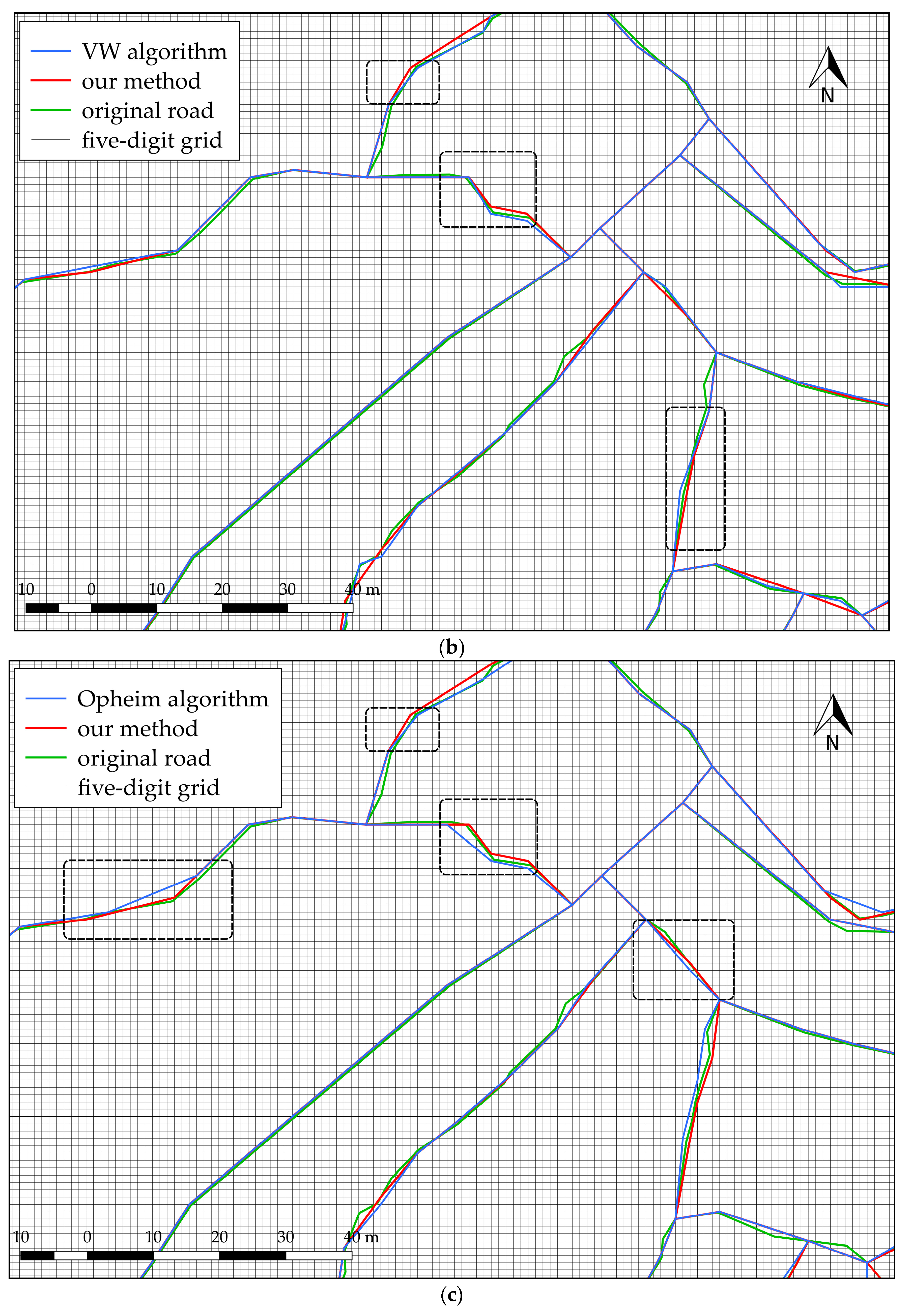
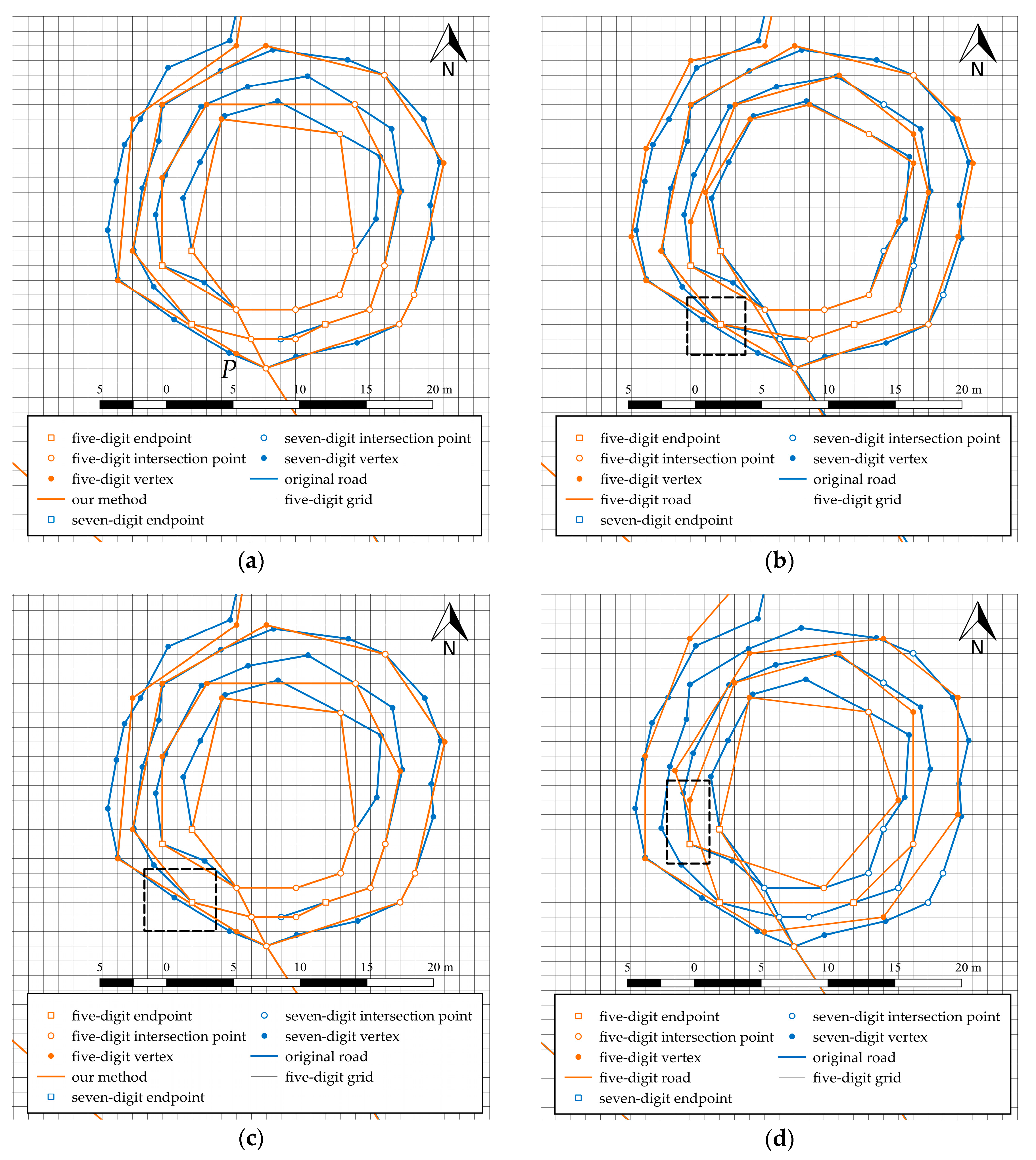
Compared with the DP, VW, and Opheim algorithms, the improved Opheim algorithm that considers requirements in navigation retains the characteristic points needed for navigation and is combined with the intelligent maintenance of the spatial directional relationship. The local shape of the roads is similar to the original roads after road data precision is reduced. In the Hausdorff distance statistics between the road networks with five-digit precision and the original road networks, the result of our method was close to the Opheim algorithm, and the difference was smaller than those of the other three methods. The average change of turning angles with local shape adjustment was optimized compared to the average change in turning angles without local shape adjustment. A part of the visual effects of the results was shown in Figure 16.

(2)

Our algorithm considers the spatial topological relationships among all features. Theoretically, in the process of maintaining the local shape of the road, when topological errors occur in all optional positions of a vertex, topological errors will be marked in the result. During the process of adjusting the spatial relationship among the roads connecting with the node, if all the schemes satisfying the user-defined constraint on spatial directional deviation cause spatial topological errors, the optimal scheme selected from them will also cause spatial topological errors.

(3)

The spatial directional relationships between roads at all nodes in road networks are maintained when data precision is lowered. The spatial directional relationship among road segments connected at every general node is adjusted optimally and total changes in azimuths of road segments connected at special nodes are minimized by obtaining the near-optimal solution.

However, the proposed method in this paper was used to extract road network maps (five digit) used for conventional navigation from high-precision road network maps (seven digit) instead of extracting maps with other precision levels. If it will be used to produce road network data with four-digit precision, then the grid width is expanded by 10 times, and the simplification and adjustment of a road network will be more difficult. In future research, we hope that this proposed algorithm becomes more intelligent to meet the requirements of road network generalization for navigation. Another future task is to study the iterative displacement method to address the spatial topological conflicts caused by road simplification, and to consider the buildings along roads to avoid inconsistencies between roads and buildings after reducing the precision.

References

1. Li, Z. Algorithmic Foundation of Multi-Scale Spatial Representation; CRC Press: Boca Raton, FL, USA, 2006. [Google Scholar]
2. Douglas, D.H.; Peucker, T.K. Algorithms for the reduction of the number of points required to represent a digitized line or its caricature. Cartogr. Int. J. Geogr. Inf. 1973, 10, 112–122. [Google Scholar] [CrossRef] [Green Version]
3. Opheim, H. Smoothing a digitized curve by data reduction methods. In Proceedings of the Eurographics, Munich, Germany, 9–11 September 1981; pp. 127–135. [Google Scholar]
4. Opheim, H. Fast data reduction of a digitized curve. Geo-Process. 1982, 2, 33–40. [Google Scholar]
5. Visvalingam, M.; Whyatt, J.D. Line generalisation by repeated elimination of points. Cartogr. J. 1993, 30, 46–51. [Google Scholar] [CrossRef]
6. Saalfeld, A. Topologically consistent line simplification with the Douglas-Peucker algorithm. Comput. Geosci. Inf. Sci. 1999, 26, 7–18. [Google Scholar] [CrossRef]
7. Pallero, J. Robust line simplification on the plane. Comput. Geosci. 2013, 61, 152–159. [Google Scholar] [CrossRef]
8. Tienaah, T.; Stefanakis, E.; Coleman, D.J.G. Contextual Douglas-Peucker simplification. Geomatica 2015, 69, 327–338. [Google Scholar] [CrossRef]
9. Qingsheng, G.; Brandenberger, C.; Hurni, L. A progressive line simplification algorithm. Geo-Spat. Inf. Sci. 2002, 5, 41–45. [Google Scholar] [CrossRef] [Green Version]
10. Park, W.; Yu, K. Hybrid line simplification for cartographic generalization. Pattern Recognit. Lett. 2011, 32, 1267–1273. [Google Scholar] [CrossRef]
11. Keates, J.S. Cartographic Design and Production; Longman Inc.: New York, NY, USA, 1973. [Google Scholar]
12. Jones, C.B.; Ware, M. Nearest neighbor search for linear and polygonal objects with constrained trianglations. In Proceedings of the 8th International Symposium on Spatial Data Handling, Vancouver, BC, Canada, 11–15 July 1998; pp. 13–21. [Google Scholar]
13. Ai, T.; Guo, R.; Liu, Y. A Binary Tree Represen tation of Curve H ierarch ical Structure in Depth. Acta Geod. Cartogr. Sin. 2001, 30, 343–348. [Google Scholar]
14. Ai, T.; Liu, Y.; Chen, J. The hierarchical watershed partitioning and data simplification of river network. In Progress in Spatial Data Handling; Springer: Berlin/Heidelberg, Germany, 2006; pp. 617–632. [Google Scholar]
15. Ai, T. The drainage network extraction from contour lines for contour line generalization. ISPRS J. Photogramm. Remote Sens. 2007, 62, 93–103. [Google Scholar] [CrossRef]
16. Ai, T.; Zhou, Q.; Zhang, X.; Huang, Y.; Zhou, M. A Simplification of Ria Coastline with Geomorphologic Characteristics Preserved. Mar. Geod. 2014, 37, 167–186. [Google Scholar] [CrossRef]
17. Ai, T.; Ke, S.; Yang, M.; Li, J. Envelope generation and simplification of polylines using Delaunay triangulation. Int. J. Geogr. Inf. Sci. 2016, 31, 297–319. [Google Scholar] [CrossRef]
18. Perkal, J. An attempt at objective generalization. Mich. Inter.-Univ. Community Math. Geogr. Discuss. Pap. 1966, 10, 130–142. [Google Scholar]
19. Li, Z.; Openshaw, S. Algorithms for automated line generalization1 based on a natural principle of objective generalization. Int. J. Geogr. Inf. Sci. 1992, 6, 373–389. [Google Scholar] [CrossRef]
20. Shi, W.; Cheung, C. Performance Evaluation of Line Simplification Algorithms for Vector Generalization. Cartogr. J. 2006, 43, 27–44. [Google Scholar] [CrossRef]
21. Lang, T. Rules for the robot draughtsmen. Comput. Geosci. 1969, 42, 50–51. [Google Scholar]
22. Rcumann, K.; Witkam, A.P.M. Optimizing curve segmentation in computer graphics. In Proceedings of the International Computing Symposium, Davos, Switzerland, 4–7 September 1973; pp. 467–472. [Google Scholar]
23. Cromley, R.G. Principal axis line simplification. Cartogr. J. 1992, 18, 1003–1011. [Google Scholar] [CrossRef]
24. Zhao, Z.; Saalfeld, A. Linear-time sleeve-fitting polyline simplification algorithms. In Proceedings of the AutoCarto 13, Seattle, WA, USA, 7–10 April 1997. [Google Scholar]
25. McMaster, R.B.; Shea, K.S. Generalization in Digital Cartography; Association of American Geographers: Washington, DC, USA, 1992. [Google Scholar]
26. De Berg, M.; van Kreveld, M.; Schirra, S. Topologically Correct Subdivision Simplification Using the Bandwidth Criterion. Cartogr. Geogr. Inf. Syst. 2013, 25, 243–257. [Google Scholar] [CrossRef]
27. Yu, J.; Chen, G.; Zhang, X.; Chen, W.; Pu, Y. An improved Douglas-Peucker algorithm aimed at simplifying natural shoreline into direction-line. In Proceedings of the 2013 21st International Conference on Geoinformatics, Kaifeng, China, 20–22 June 2013; pp. 1–5. [Google Scholar]
28. Goyal, R.K.; Egenhofer, M.J. Similarity Assessment for Cardinal Directions between Extended Spatial Objects; University of Maine: Orono, ME, USA, 2000. [Google Scholar]
29. Goyal, R.K.; Egenhofer, M.J. Consistent queries over cardinal directions across different levels of detail. In Proceedings of the 11th International Workshop on Database and Expert Systems Applications, Washington, DC, USA, 10–13 September 2000; pp. 876–880. [Google Scholar]
30. Tang, L.; Yang, B.; Xu, K. The Road Data Change Detection Based on Linear Shape Similarity. Geomat. Inf. Sci. Wuhan Univ. 2008, 33, 367–370. [Google Scholar]
31. Tang, L.; Li, Q.; Xu, F.; Chang, X. One new method for road data shape change detection. In Proceedings of the International Symposium on Spatial Analysis, Spatial-Temporal Data Modeling, and Data Mining, Wuhan, China, 13 October 2009; p. 749209. [Google Scholar]
32. Chehreghan, A.; Ali Abbaspour, R. An assessment of spatial similarity degree between polylines on multi-scale, multi-source maps. Geocarto Int. 2017, 32, 471–487. [Google Scholar] [CrossRef]
33. Yang, B. A multi-resolution model of vector map data for rapid transmission over the Internet. Comput. Geoences 2005, 31, 569–578. [Google Scholar] [CrossRef]
34. Yan, H.; Zhang, L.; Wang, Z.; Yang, W.; Liu, T.; Zhou, L. Quantitative Expressions of Spatial Similarity in Multi-scale Map Spaces. In Proceedings of the International Cartographic Conference, Washington, DC, USA, 2–7 July 2017; pp. 405–416. [Google Scholar]
35. Lewis, J.A.; Egenhofer, M.J. Point Partitions: A Qualitative Representation for Region-Based Spatial Scenes in ℝ2. In Proceedings of the International Conference on Geographic Information Science, Montreal, QC, Canada, 27–30 September 2016. [Google Scholar]
36. Buttenfield, B.P. Transmitting Vector Geospatial Data across the Internet. In Proceedings of the International Conference on Geographic Information Science, Boulder, CO, USA, 25–28 September 2002; pp. 25–28. [Google Scholar]
37. Guo, Q.; Liu, Y.; Li, M.; Cheng, X.; He, J.; Wang, H.; Wei, Z. A progressive simplification method of navigation road map based on mesh model. Acta Geod. Cartogr. Sin. 2019, 48, 1357–1368. [Google Scholar] [CrossRef]
38. Chai, Z.; Liang, S. A node-priority based large-scale overlapping community detection using evolutionary multi-objective optimization. Evol. Intell. 2020, 13, 59–68. [Google Scholar] [CrossRef]
39. Rosvall, M.; Bergstrom, C.T. Maps of random walks on complex networks reveal community structure. Proc. Natl. Acad. Sci. USA 2008, 105, 1118–1123. [Google Scholar] [CrossRef] [Green Version]
40. Fortunato, S. Community detection in graphs. Phys. Rep. 2010, 486, 75–174. [Google Scholar] [CrossRef] [Green Version]
41. Newman, M.E. Modularity and community structure in networks. Proc. Natl. Acad. Sci. USA 2006, 103, 8577–8582. [Google Scholar] [CrossRef] [Green Version]
42. Yu, W.; Zhang, Y.; Ai, T.; Guan, Q.; Chen, Z.; Li, H. Road network generalization considering traffic flow patterns. Int. J. Geogr. Inf. Sci. 2019. [Google Scholar] [CrossRef]
43. De Jong, K.A. Analysis of the Behavior of a Class of Genetic Adaptive Systems; University of Michigan: Ann Arbor, MI, USA, 1975. [Google Scholar]
44. Zoraster, S. Practical results using simulated annealing for point feature label placement. Int. J. Geogr. Inf. Sci. 1997, 24, 228–238. [Google Scholar] [CrossRef]
45. Ware, J.M.; Jones, C.B.; Thomas, N. Automated map generalization with multiple operators: A simulated annealing approach. Int. J. Geogr. Inf. Sci. 2003, 17, 743–769. [Google Scholar] [CrossRef]
46. Ware, J.M.; Wilson, I.D.; Ware, J.A. A knowledge based genetic algorithm approach to automating cartographic generalisation. In Applications and Innovations in Intelligent Systems X; Springer: Berlin/Heidelberg, Germany, 2003; pp. 33–49. [Google Scholar]
47. Li, Z.; Yan, H.; Ai, T.; Chen, J. Automated building generalization based on urban morphology and Gestalt theory. Cartogr. Int. J. Geogr. Inf. 2004, 18, 513–534. [Google Scholar] [CrossRef]
48. Holland, J.H. Adaptation in Natural and Artificial Systems: An Introductory Analysis with Applications to Biology, Control, and Artificial Intelligence; MIT Press: Cambridge, MA, USA, 1992. [Google Scholar]
49. Dubuisson, M.; Jain, A.K. A modified Hausdorff distance for object matching. In Proceedings of the 12th International Conference on Pattern Recognition, Jerusalem, Israel, 9–13 October 1994; pp. 566–568. [Google Scholar]
Figure 1. Roads with different precision.
Ijgi 09 00490 g001
Figure 2. The main steps of our method.
Ijgi 09 00490 g002
Figure 3. Representation model of a road network: (a) road and (b) road network G.
Ijgi 09 00490 g003
Figure 4. Spatial directional relationship with different precision: (a) the azimuth of segment V i P i + 1 at node Vi; (b) the turning angle between two sequential road segments at vertex Pi.
Ijgi 09 00490 g004
Figure 5. Maintenance of road spatial directional relationship. Road segments associated with (a) a general node and (b) the vertex.
Ijgi 09 00490 g005
Figure 6. Mapping from a local subgroup of the road network to chromosome.
Ijgi 09 00490 g006
Figure 7. Topological conflict: (a) vertex elimination and (b) maintenance of spatial directional relationship.
Ijgi 09 00490 g007
Figure 8. Height changes along a road topographic feature.
Ijgi 09 00490 g008
Figure 9. Extraction of a long, straight and flat road section.
Ijgi 09 00490 g009
Figure 10. The Opheim algorithm for polyline simplification.
Ijgi 09 00490 g010
Figure 11. Vertex elimination on a curved road. (a) Di,1 < ε; (b) Di,1ε; (c) Di,1ε and Di,2ε; (d) Di,1ε and Di,2 < ε; (e) Di,1ε, Di,2 < ε and Di + 1,2ε; (f) Di,1ε, Di,2 < ε and Di + 1,2 < ε; (g) |Ti| <= |Ti + 1| based on (e); (h) |Ti| > |Ti + 1| based on (e); (i) |Ti| < θ based on (f); (j) |Ti| <= |Ti + 1| based on (f); (k) |Ti| > |Ti + 1| based on (f).
Ijgi 09 00490 g011
Figure 12. Connection situations of a general node: (a) two excluded connection situations; (b) optimal connection situation.
Ijgi 09 00490 g012
Figure 13. Maintenance of the spatial directional relationship at special nodes. The blue line represents the original road and the orange line represents the road with five-digit precision. (a) Original data with seven-digit precision, (b) adjustment from V1 to V2, and (c) adjustment from V2 to V1.
Ijgi 09 00490 g013
Figure 14. Gene crossover process.
Ijgi 09 00490 g014
Figure 15. Seven-digit original road network data of a region in Chongqing, China. The region in red box 1 is shown in Figure 16, and the region in red box 2 is shown in Figure 17.
Ijgi 09 00490 g015
Figure 16. Simplified results of different algorithms. Comparison of (a) the DP algorithm and the improved Opheim algorithm; (b) the VW algorithm and the improved Opheim algorithm; (c) the Opheim algorithm and the improved Opheim algorithm.
Ijgi 09 00490 g016aIjgi 09 00490 g016b
Figure 17. Simplified results of different algorithms: (a) improved Opheim; (b) DP; (c) VW, and (d) Opheim algorithms.
Ijgi 09 00490 g017
Figure 18. Maintenance of spatial directional relationship at special nodes using e-GA. The blue line represents the original road and the orange line represents the road with five-digit precision. V1 and V2 are nodes.
Ijgi 09 00490 g018