
Robust Estimation and Forecasting of Climate Change Using Score-Driven Ice-Age Models


1
School of Business, Universidad Francisco Marroquín, Guatemala 01010, Guatemala
2
Department of Economics, Universidad Carlos III de Madrid, Calle Madrid 126, 28903 Getafe, Spain
*
Author to whom correspondence should be addressed.
Econometrics 2022, 10(1), 9; https://0-doi-org.brum.beds.ac.uk/10.3390/econometrics10010009
Submission received: 19 October 2021
/
Revised: 21 January 2022
/
Accepted: 11 February 2022
/
Published: 16 February 2022
(This article belongs to the Collection Econometric Analysis of Climate Change)
Abstract
:We use data on the following climate variables for the period of the last 798 thousand years: global ice volume (), atmospheric carbon dioxide level (), and Antarctic land surface temperature (). Those variables are cyclical and are driven by the following strongly exogenous orbital variables: eccentricity of the Earth’s orbit, obliquity, and precession of the equinox. We introduce score-driven ice-age models which use robust filters of the conditional mean and variance, generalizing the updating mechanism and solving the misspecification of a recent climate–econometric model (benchmark ice-age model). The score-driven models control for omitted exogenous variables and extreme events, using more general dynamic structures and heteroskedasticity. We find that the score-driven models improve the performance of the benchmark ice-age model. We provide out-of-sample forecasts of the climate variables for the last 100 thousand years. We show that during the last 10–15 thousand years of the forecasting period, for which humanity influenced the Earth’s climate, (i) the forecasts of are above the observed , (ii) the forecasts of level are below the observed , and (iii) the forecasts of are below the observed . The forecasts for the benchmark ice-age model are reinforced by the score-driven models.
1. Introduction
According to Intergovernmental Panel on Climate Change (2021), compared to the period of 1850–1900, the Earth’s global surface temperature for the period of 2081–2100 will very likely rise by 3.3 to 5.7 °C under the worst-case scenario, which implies dramatic consequences on the nature and wildlife in terrestrial, wetland, and ocean ecosystems, and on humanity with respect to food and water security, migration, health, higher risk of conflict worldwide, reduction of global economic product, and a possible collapse of the current societal organization. Climate change is partly due to the influence of humanity, which started approximately 10–15 thousand years ago, by commencing agricultural activities such as cultivating plants and livestock (Ruddiman 2005). That influence has significantly increased since the industrial revolution (1769–1840), when human activities such as burning fossil fuels (e.g., coal and oil) have importantly increased, and the influence of humanity has further increased with an accelerating growth rate since then. The Earth’s population rose from 1 billion in 1800 to more than 7.8 billion in 2021, which was associated with a significant global-scale economic expansion. One of the consequences is the rising greenhouse gas emissions (e.g., carbon dioxide, , nitrous oxide, , and methane, ), which are directly related to global warming.
The atmospheric levels and land surface temperature are related to melting glaciers and sea ice. We name the climate–econometric models of those variables as ice-age models, as per the work of Castle and Hendry (2020). During the 4.5 billion-year history of the Earth, the ice volume, atmospheric , and land surface temperature simultaneously changed, driven by exogenous orbital variables, such as (i) changes in the non-circularity of the Earth’s orbit with a period of 100 thousand years, (ii) changes in the tilt of the Earth’s rotational axis relative to the ecliptic (i.e., the plane of the Earth’s orbit around the Sun) with a period of 41 thousand years, and (iii) circular rotation of the rotational axis itself, which changes the season at which the Earth’s orbit is nearest to the Sun, with a period that is between 19 to 23 thousand years (it is variable due to the changes in the tilt of the rotational axis).
As in the work of Castle and Hendry (2020), we use data for climate and orbital variables for the period of the last 798 thousand years, where the climate variables in the model are global ice volume, atmospheric , and Antarctic land surface temperature. The orbital variables (i) to (iii) are exogenous to humanity and are included in the ice-age models. There are additional exogenous variables which may also influence the Earth’s climate and are omitted, such as: (iv) variations in the Sun’s radiation output, (v) volcanic eruption particles in the atmosphere and ice cover, and (vi) changes in the magnetic poles. The new ice-age models of the present paper consider error term specifications that allow for fat-tails and heteroskedasticity, to control for the omitted variables (iv) to (vi).
The main objective of this work is to study the robustness of the results of Castle and Hendry (2020). We improve the model specification of those authors using more general score-driven updates of location and scale in the ice-age model. Score-driven time series models are introduced in the works of Creal et al. (2008) and Harvey and Chakravarty (2008). Those authors name the score-driven models as: generalized autoregressive score (GAS) and dynamic conditional score (DCS) models, respectively. Score-driven models are observation-driven models (Cox 1981), in which the filters are updated using the scaled conditional score functions of the log-likelihood (LL) of the dependent variables.
The use of the score-driven ice-age models is motivated as follows: (i) The updating mechanisms of those models are generalizations of those of the classical time series models such as: ARMA (autoregressive moving average) (Box and Jenkins 1970), GARCH (generalized autoregressive conditional heteroskedasticity) (Engle 2002; Bollerslev 1986), and VARMA (vector ARMA) (Tiao and Tsay 1989). Hence, the score-driven ice-age models of the present paper are extensions of the VAR with explanatory variables (VARX) model of Castle and Hendry (2020). (ii) Score-driven models are robust to outliers and missing observations (Harvey 2013). Hence, the score-driven ice-age models may control for the effects of the omitted exogenous variables. (iii) A score-driven update, asymptotically at the true values of parameters, locally reduces the Kullback–Leibler distance between the true and the estimates values of the score-driven filter in every step, and only score-driven models have this property (Blasques et al. 2015). Hence, score-driven filters use an information-theoretically optimal updating mechanism. We note that the linear updating mechanisms of ARMA and VARMA, and the quadratic updating mechanism of GARCH are optimal from an information-theoretic perspective only if the data generating process (DGP) has a normal distribution. (iv) Under a correct model specification, asymptotically, and at the true values of parameters, the updating terms of the score-driven models are martingale difference sequences (MDS) (Harvey 2013). For the multivariate t-distribution of the present paper, under the same conditions, the same updating terms are white noise processes, due to the well-defined covariance matrix of errors. In the empirical application, we perform model specification tests which support the use of the most general score-driven ice-age model of this paper.
These advantages of the score-driven models motivate their application to climate data. We compare the statistical and forecasting performances of the ice-age model of Castle and Hendry (2020) with those of our score-driven ice-age models. We also report impulse responses among global ice volume, atmospheric level, and Antarctic land surface temperature, which are robust for the ice-age model of Castle and Hendry (2020). Likelihood-based model performance metrics, diagnostic tests, and forecasting results indicate that the model of Castle and Hendry (2020) is improved.
Using data for the first 698 thousand years of the sample (for which humanity did not influence the Earth’s climate), we present out-of-sample forecasts of the global ice volume, atmospheric level, and Antarctic land surface temperature for the period of the last 100 thousand years of the sample. We find that the forecasting results of Castle and Hendry (2020) are robust. For the last 10–15 thousand years of the forecasting period, we find that: (i) the forecasts of global ice volume are above the observed global ice volume, (ii) the forecasts of the atmospheric level are below the observed level, and (iii) the forecasts of Antarctic land surface temperature are below the observed Antarctic land surface temperature.
2. Climate Econometrics
2.1. Benchmark Ice-Age Model
Model specification—In the work of Castle and Hendry (2020, chp. 6), estimation and forecasting results are presented for a general unrestricted model (GUM), named the ice-age model. That model specification is the benchmark model of the present paper. The dependent variables of the ice-age model are , where ‘Ice’ denotes global ice volume, ‘’ denotes atmospheric carbon dioxide level, and ‘Temp’ denotes Antarctic-based land surface temperature. The order of the variables in is defined in the work of Castle and Hendry (2020), which we use for all models of the present paper. Correspondingly, the ice-age model is specified as follows:
where is the conditional mean of given , the reduced-form error term has a multivariate i.i.d. normal distribution, where the covariance matrix is (), for which () is a lower triangular matrix with positive elements in the diagonal, and includes strongly exogenous explanatory variables. We initialize using the start values of the dependent variables . We assume that the maximum modulus of the eigenvalues of , denoted as , is less than one. The elements of the vector of explanatory variables are three interacting orbital changes over time affecting solar radiation:
where ‘Ec’ measures the eccentricity (i.e., non-circularity) of the Earth’s orbit, ‘Ob’ is obliquity measuring the tilt of the Earth’s rotational axis relative to the ecliptic, and ‘Pr’ is a measure of the precession of the equinox (i.e., circular rotation of the rotational axis itself).
The conditional mean in Equation (1) includes the vector of constant parameters , and parameter matrices (), (), and (). For the benchmark ice-age model, we report estimation and forecasting results for Equation (1) which excludes the outlier-dummies. The same outlier-dummies are also excluded from the score-driven ice-age models of the present paper, because those models are robust to extreme observations (Harvey 2013).
The GUM estimates reported in the work of Castle and Hendry (2020, p. 104) impose restrictions on the matrices , , and . According to those restrictions, the following elements of are not restricted to zero: , , , , , and . Additionally, the following elements of are not restricted to zero: , , , , , , , and . Furthermore, the following elements of are also not restricted to zero: , , , , , , and . The benchmark ice-age model is estimated using the maximum likelihood (ML) method.
Impulse responses—We estimate the dynamic effects of the i.i.d. structural-form error term . The corresponding IRFs are defined as follows:
The IRFs are identified using the sign restrictions for the contemporaneous effects among the elements of , which are based on simulations of matrix , according to the following procedure (Rubio-Ramirez et al. 2010): (i) A matrix of independent numbers is simulated. (ii) The QR decomposition of is performed, and the resulting matrices are denoted as (orthogonal matrix) and (upper triangular matrix). (iii) We define , for which the estimates of are used. For the IRFs, 3 million simulations of are generated, and only those simulations are used that satisfy the sign restrictions of Table 1, and for each simulation is replaced by in the IRF formulas. For the simulations that satisfy the sign restrictions, we report the mean ± one standard deviation estimates of the IRFs. The sign restrictions of Table 1 are motivated as follows:
(i) In the work of Castle and Hendry (2020) the correlation coefficient estimates among the residuals of the ice-age model are reported, which motivate the sign restrictions of Table 1. (ii) For the negative effects of on , and for the positive effects of on of Table 1, we refer to the work of Qin and Buehler (2012). For the positive interaction effects between and of Table 1, we also refer to the works of Jouzel et al. (2007) and Lüthi et al. (2008). (iii) For the negative effects of on of Table 1, we refer to the work of Wadham et al. (2019). (iv) For the positive effects of on of Table 1, we refer to the work of Archer et al. (2004). (v) For the negative interaction effects between and of Table 1, we refer to the work of Bronselaer et al. (2018).
2.2. Score-Driven Ice-Age Models
Castle and Hendry (2020, p. 102) recognize that the benchmark ice-age model suffers from residual autocorrelation. This may be due to omitted exogenous variables, such as the Sun’s radiation output or changes in the Earth’s magnetic poles. This may also be due to the presence of heteroskedasticity generated by the omitted variables, which might cause fat-tails in the error distribution. There are alternative ways to address those misspecification issues from an econometric perspective. In this paper, we address those issues using the flexible and robust class of score-driven models.
2.2.1. Score-Driven Homoskedastic Ice-Age Model
Model specification—The score-driven ice-age model of this paper uses the score-driven model specification in the work of Harvey (2013, p. 56). The model is specified as follows:
where is the conditional mean of given , is the multivariate i.i.d. reduced-form error term, is the vector of strongly exogenous explanatory variables, and is the vector of scaled score functions (Harvey 2013). The assumption of strict exogeneity of is from the work of Harvey (2013, p. 56), which is supported for of Equation (2) in the work of Castle and Hendry (2020, p. 95). We initialize using the start values of the dependent variables (Harvey 2013). The conditional mean includes the vector of constant parameters , and the parameter matrices (), (), (), and (). We assume that the maximum modulus of the eigenvalues of , denoted as , is less than one.
For , , and , we use the restrictions of Castle and Hendry (2020), a decision which is motivated by the following general-to-specific model selection procedure. First, for the parameter estimation of the score-driven ice-age model, we start with the aforementioned restrictions of and , and we use unrestricted parameter matrices for and . Second, we restrict those parameters of and to zero which are not significant at the 1% level. The same elements of and are restricted for the score-driven models as for matrix in the work of Castle and Hendry (2020). Hence, the following elements of are not restricted to zero: , , , , , and .
The reduced-form error term has a multivariate i.i.d. t-distribution, where the scale matrix is (), for which () is a lower triangular squared matrix with positive elements in the diagonal, and is the degrees of freedom parameter (the restriction on the parameter space ensures that the covariance matrix of is well-defined).
The scaled score function is defined as follows. The log of the conditional density of is:
where , is the vector of time-invariant parameters, which includes the elements of , , , , , , and . The partial derivative of the log conditional density with respect to is (Harvey 2013):
The scaled score function is defined in the second equality of Equation (7), where is multiplied by . Therefore, the scaled score function is bounded by the reduced-form error term: . All elements of are bounded functions of for (Harvey 2013), hence all moments of are well-defined. In the work of Harvey (2013), it is shown that is multivariate i.i.d. with mean zero and a covariance matrix:
We also note that if , then . In the limiting case, Equations (3) and (4) provide a VARMAX(1,1) structure for the dependent variables:
The benchmark ice-age model is a special case of the score-driven ice-age model, because if and for Equations (4) and (5), then we obtain Equation (1). This can also be seen for the limiting case for in Equation (9), using . We name Equation (9) the score-driven homoskedastic Gaussian ice-age model.
All score-driven models are estimated using the ML method. For the ML estimation, we assume correct model specifications for all econometric models of the present paper. Under that assumption, the standard errors of the ML estimates are consistently estimated using the outer product of the gradient of the LL function. Another consequence of the correct model specification assumption is that the updating terms of the score-driven filters of this paper, asymptotically and at the true values of parameters, are white noise vectors. For technical details on the statistical inference of score-driven models, we refer to the works of Harvey and Chakravarty (2008), Harvey (2013), Creal et al. (2008, 2011, 2013), and Blasques et al. (2021). For the multivariate score-driven models (such as the score-driven ice-age models), we also refer to the recent works of Blazsek et al. (2020, 2021a, 2021b).
Impulse responses—First, we define the vector of the structural-form error terms (). The variance of the reduced-form error term is factorized, as follows:
Based on that, the following multivariate i.i.d. structural-form error term is introduced:
where , and .
Furthermore, by substituting Equation (11) into Equation (7), as a function of the structural-form error term is:
Second, from Equations (4) and (5), the nonlinear MA(∞) representation of is:
We focus on the impulse responses for the dependent variables , because the variables within are strongly exogenous to humanity. From , we are particularly interested in the dynamic effects of the atmospheric carbon dioxide level on the Antarctic-based land surface temperature, because humanity has influence on the emissions. Thus, the new measurement method of impulse responses for the score-driven ice-age model of this paper may have policy implications in relation to carbon dioxide emissions regulation. The contemporaneous and dynamic effects of the structural-form error term , respectively, are given by the following equations:
where
We compare the IRFs of the score-driven ice-age models and the IRFs of the benchmark ice-age model, which are not reported in the work of Castle and Hendry (2020). In Equation (15), the dynamic interaction effects are time-dependent due to . In the empirical application of the present paper, we replace by the sample average (White 2001), where the sample average is estimated for the last 10 observations of the sample, motivated by the work of Castle and Hendry (2020, p. 111). There are alternative ways for the estimation of dynamic interaction effects for nonlinear models (Lütkepohl 2005), hence the IRF estimation of our paper may be modified in future applications.
Finally, we also report contemporaneous and dynamic effects of the structural-form error term for the score-driven ice-age model for the multivariate normal distribution:
The IRFs of this section are identified using the procedure of Rubio-Ramirez et al. (2010).
2.2.2. Score-Driven Heteroskedastic Ice-Age Model
Model specification—We extend the score-driven ice-age model for the homoskedastic multivariate t-distribution, by considering score-driven conditional heteroskedasticity with constant correlation coefficients for the reduced-form error term . The model is specified as follows:
where is the conditional mean of given , which is defined later in this section, is the multivariate i.i.d. reduced-form error term, is the vector of strongly exogenous explanatory variables, and is the vector of scaled score functions. We initialize using (Harvey 2013). The conditional mean includes the vector of constant parameters , and the parameter matrices (), (), (), and (). For the parameters of , we use the same restrictions as for the homoskedastic score-driven ice-age model for the t-distribution. We assume that the maximum modulus of the eigenvalues of , denoted as , is less than one.
The reduced-form error term has a multivariate conditional t-distribution, where degrees of freedom , the scale matrix is , where () is a time-varying diagonal matrix with the score-driven scales of each time series, and R () is the time-invariant correlation matrix. This specification assumes that the correlation coefficients are constant over time, which can be extended according to the results of Creal et al. (2011) to dynamic correlation coefficients, using a score-driven volatility plus correlation model for the t-distribution.
The positive definiteness of R and boundedness of the correlation coefficients for are ensured using the following specification: , where () is a diagonal matrix in which the elements of the diagonal are the square roots of the elements of the diagonal of the positive definite matrix Q () (Engle 2002). The positive definiteness of Q is ensured using the Cholesky decomposition , in which () is a lower triangular matrix with positive elements in the diagonal. For parameter identification reasons, each element of the diagonal of is restricted to one. Furthermore, is specified as follows:
We specify the filters in Equation (21) as follows:
where is the signum function, and for measure asymmetric effects in the conditional scale of the dependent variables. We initialize for using the unconditional mean for , respectively (Harvey 2013). In the following, we define the updating terms and . For the covariance stationarity of , asymptotically at the true values of parameters, it is required that for .
First, the scaled score function is defined as follows. The log conditional density of is:
where , , is the vector of constant parameters, which includes the elements of , , , , , , , , , , , , , , , , , , and . The partial derivative of with respect to is:
The scaled score function is defined in the second equality of Equation (24), where is multiplied by . Therefore, the scaled score function is bounded by the reduced-form error term: . All elements of are bounded functions of for , hence all moments of are well-defined. The scaled score function has a zero conditional mean and the following conditional covariance matrix:
Second, the updating term for is defined as follows. The conditional distributions of the marginals of are for (Kibria and Joarder 2006). The log of the conditional density of for is
where . We define the updating term of the filter for as follows:
Equations (22) and (27) are the Beta-t-EGARCH with leverage effects model of Harvey and Chakravarty (2008) (see also Creal et al. 2013 and Harvey 2013).
Impulse responses—First, we define the structural-form error terms (). The conditional variance of the reduced-form error term is factorized, as follows:
Based on that, the following multivariate i.i.d. structural-form error term is introduced:
where , and . Furthermore, by substituting Equation (29) into Equation (24), as a function of the structural-form error term is:
Second, from Equations (19) and (20), the nonlinear MA(∞) representation of is:
The contemporaneous and dynamic effects of the structural-form error term , respectively, are:
where is given by Equation (16). In Equations (32) and (33), the dynamic interaction effects are time-dependent due to and . We replace and by their sample averages for the last 10 observations of the sample. The IRFs are identified using the procedure of Rubio-Ramirez et al. (2010). We also refer to the work of Lütkepohl (2005) for alternative estimation methods.
3. Empirical Results
3.1. Data
The dependent variables of this study are global ice volume , atmospheric , and Antarctic land surface temperature . The data source of global ice volume is in the work of Lisiecki and Raymo (2005), in which time series of the , obtained from calcium carbonate () shells of foraminifera, are used to approximate temperature. Those authors use benthic records of foraminifera from seafloor sediment, which are collected at 57 globally distributed sites. Those sites are well-distributed in latitude, longitude, and depth in the Atlantic, Pacific, and Indian Oceans. The data source of atmospheric is in the work of Lüthi et al. (2008), in which changes in past atmospheric concentrations are determined by measuring the composition of air trapped in ice cores from Antarctica. Within the European Project for Ice Coring in Antarctica (EPICA), two deep ice cores have been drilled at the Kohnen Station and the Concordia Station (Dome C). The drillings were stopped at, or a few meters above, bedrock at a depth of 2774 m and 3270 m, respectively. The data source of Antarctic land surface temperature is in the work of Jouzel et al. (2007), in which temperature data were obtained within the EPICA at the Concordia Station (Dome C), using deuterium measurements from the surface down to 3259.7 m.
The exogenous explanatory variables of this study are eccentricity of the Earth’s orbit, obliquity of the Earth’s rotational axis relative to the ecliptic, and precession of the equinox. The source of those data is in the work of Paillard et al. (1996), in which the AnalySeries software is used, to provide measurements of eccentricity, obliquity, and precession.
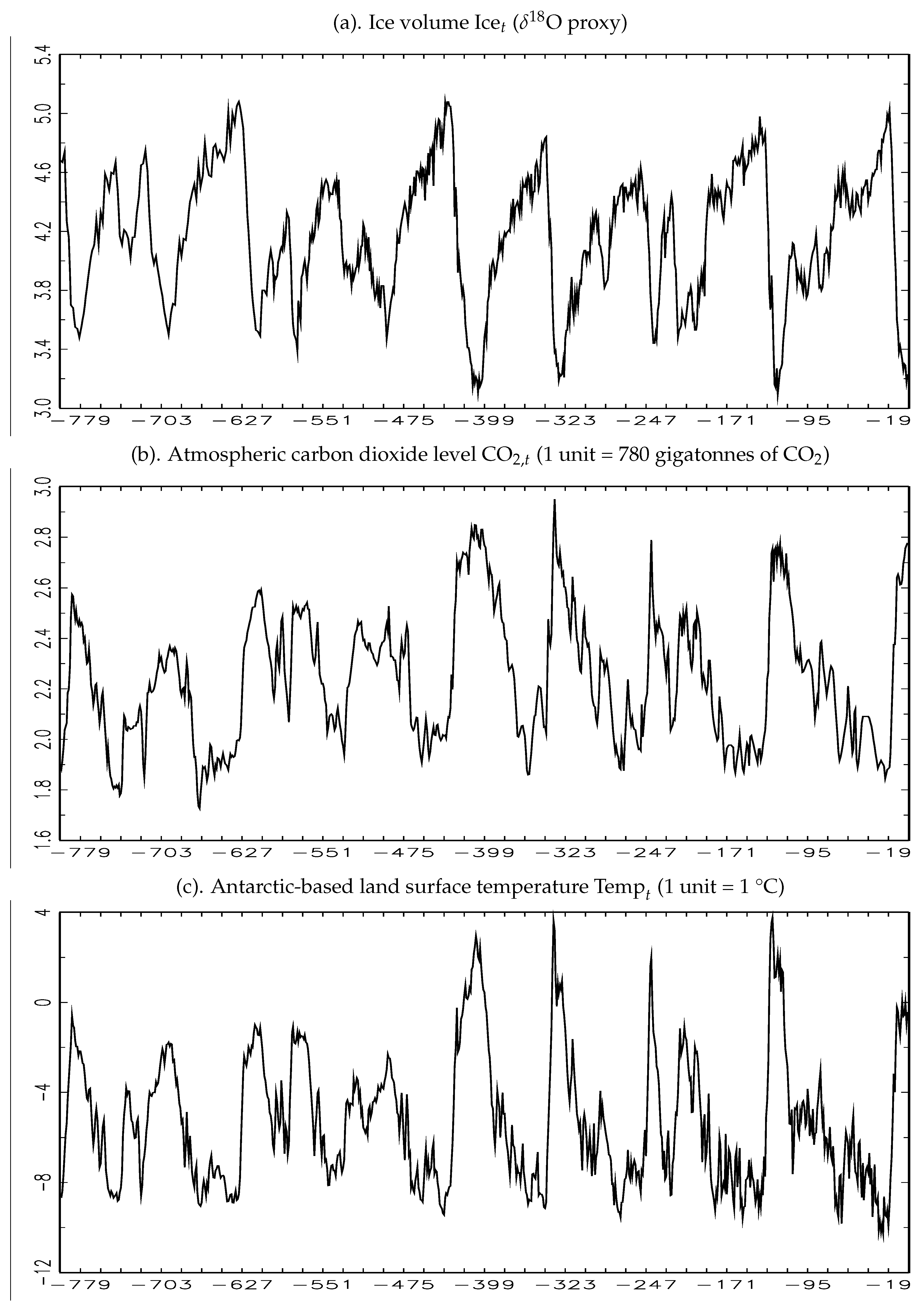
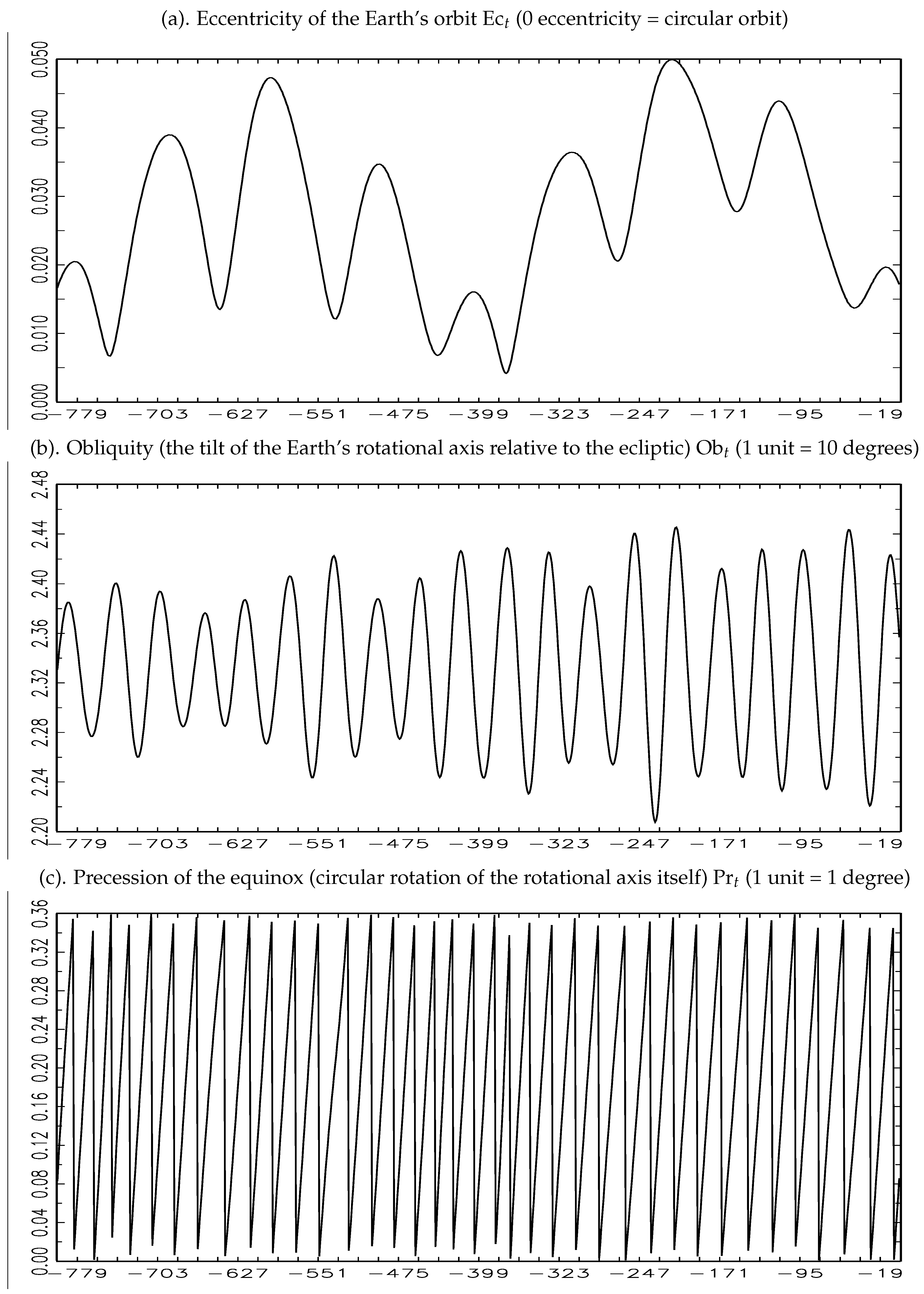
In Table 2, the descriptive statistics of the dependent and the explanatory variables are presented. The table shows the definition of each variable, observation period, units of measurement, data sources, and some additional descriptive statistics. In Figure 1 and Figure 2, the evolution of the dependent and explanatory variables, respectively, are presented. According to Figure 1b,c, atmospheric and Antarctic land surface temperature , respectively, remarkably are in unison. In Figure 1, it can also be noticed that global ice volume moves in the opposite direction from and , creating the ice-age and inter-glacial periods periodically. The seasonality of the dependent variables (Figure 1), which is due to the three main interacting orbital changes over time affecting solar radiation (Figure 2), is clearly observed in these figures.
Additional explanatory variables, which are exogenous to humanity are omitted from the econometric models of this paper. For example, the following variables are omitted: (i) the variations in the Sun’s radiation output, (ii) volcanic eruption particles in the atmosphere and ice cover, and (iii) changes in the magnetic poles. In Appendix A, we present details of those exogenous variables, and we also present why those variables are not included in the climate–econometric models.
3.2. Estimation Results
In Table 3, the ML parameter estimates for the (i) benchmark ice-age model, (ii) score-driven homoskedastic ice-age model for the normal distribution, (iii) score-driven homoskedastic ice-age model for the t-distribution, and (iv) score-driven heteroskedastic ice-age model for the t-distribution are reported. According to the table, the parameters for , , , and for all models are significantly different from zero. For model (iv), significant and asymmetric volatility dynamics are estimated, as and for , and for , are significantly different from zero.
In Table 4, the statistical performance metrics and some diagnostic test results for the models of Table 3 are reported. The statistical performances are compared using the LL, Akaike information criterion (AIC), Bayesian information criterion (BIC), and Hannan–Quinn criterion (HQC) metrics (Harvey 2013, p. 56). The statistical performance of the score-driven heteroskedastic ice-age model for the t-distribution is superior to the statistical performances of other specifications of Table 3 and Table 4. For all models, the and for statistics support the covariance stationarity of and , respectively. As a diagnostic test of the residuals, we use the Ljung–Box test (Ljung and Box 1978) for all elements of , , , and . The diagnostic tests for the score functions , and are motivated by the work of Harvey (2013, p. 55), due to the robustness to extreme observations of the score-function-based Ljung–Box test. The Ljung–Box test results indicate that the ice-age model of Castle and Hendry (2020) is not fully supported, which is noted in the same work (p. 102, footnote 4). From the score-driven ice-age specifications, full support is provided for the most general score-driven heteroskedastic ice-age model for the t-distribution.
In the following, we present the parameter estimates for the benchmark ice-age model (Equation (1)) and the score-driven heteroskedastic ice-age model for the t-distribution (Equation (20)). First, the estimates of Equation (1) are given by (Table 3):
The estimates correspond to the estimates of Castle and Hendry (2020, p. 104). Second, the estimates of Equation (20) are given by (Table 3):
To compare the parameter estimates of Equations (34)–(36) with those of Equations (37)–(39), the dynamic interaction effects for global ice volume, atmospheric , and Antarctic land surface temperature are studied using the IRFs.
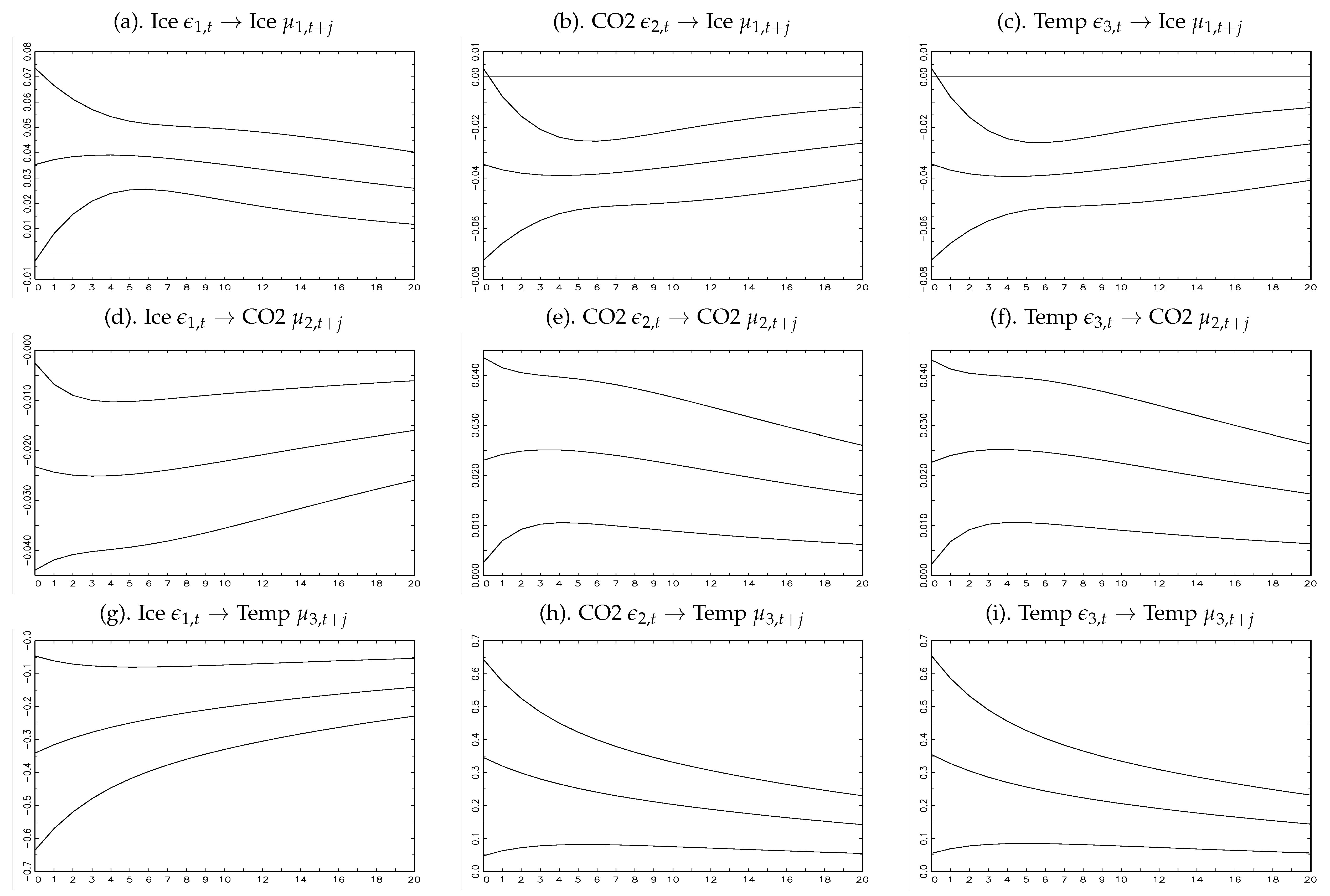
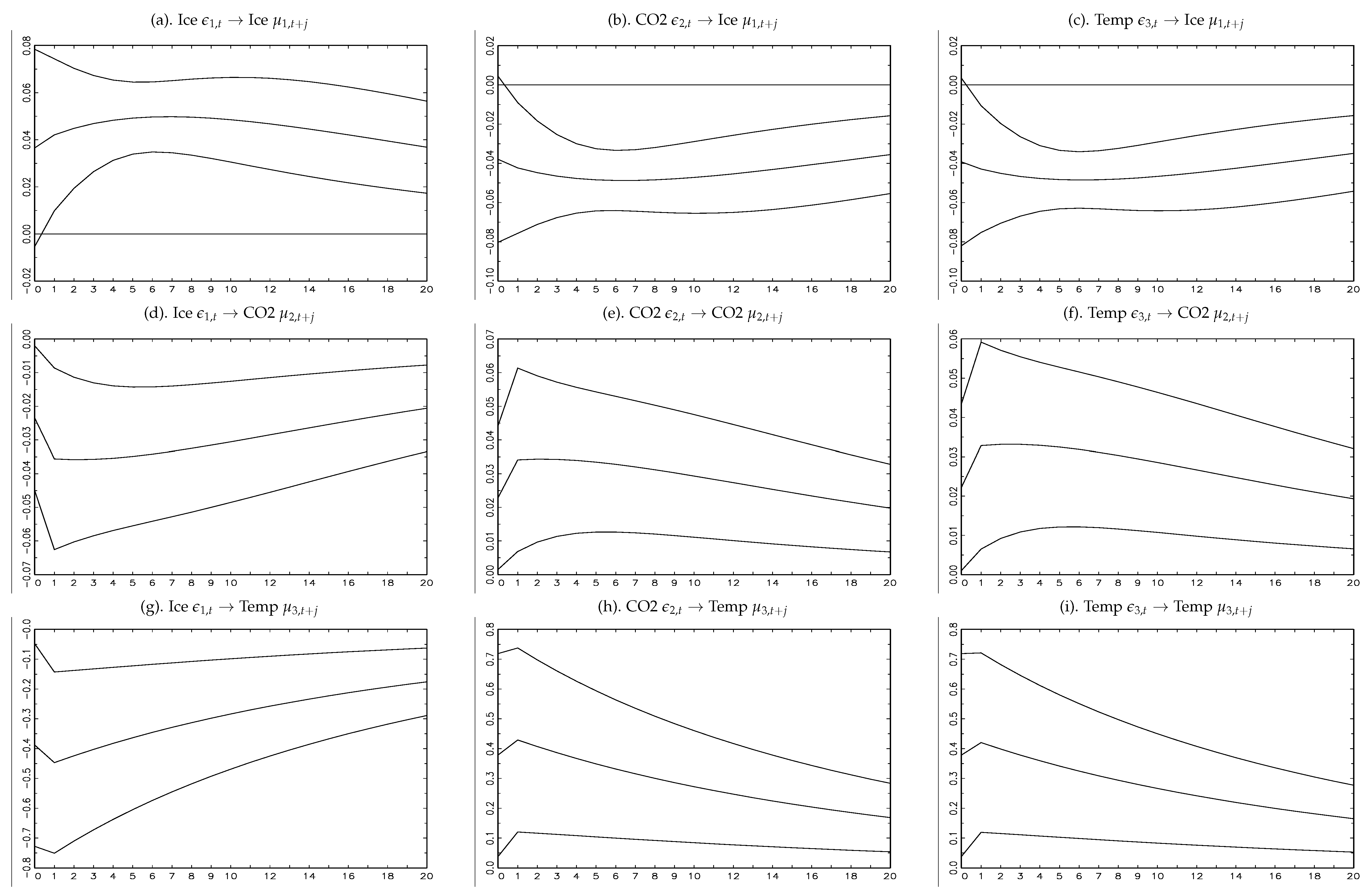
In Figure 3, Figure 4, Figure 5 and Figure 6, the IRFs for the (i) benchmark ice-age model, (ii) score-driven homoskedastic ice-age model for the normal distribution, (iii) score-driven homoskedastic ice-age model for the t-distribution, and (iv) score-driven heteroskedastic ice-age model for the t-distribution, respectively, are reported. The IRF figures indicate that the signs of the dynamic interaction effects are coherent with the signs of the same effects of the aforementioned works of Archer et al. (2004), Jouzel et al. (2007), Lüthi et al. (2008), Qin and Buehler (2012), Bronselaer et al. (2018), Wadham et al. (2019), and Castle and Hendry (2020). The IRF estimates are persistent and are consistent with the estimates of the long-run solutions of Equation (1) reported in the work of Castle and Hendry (2020).
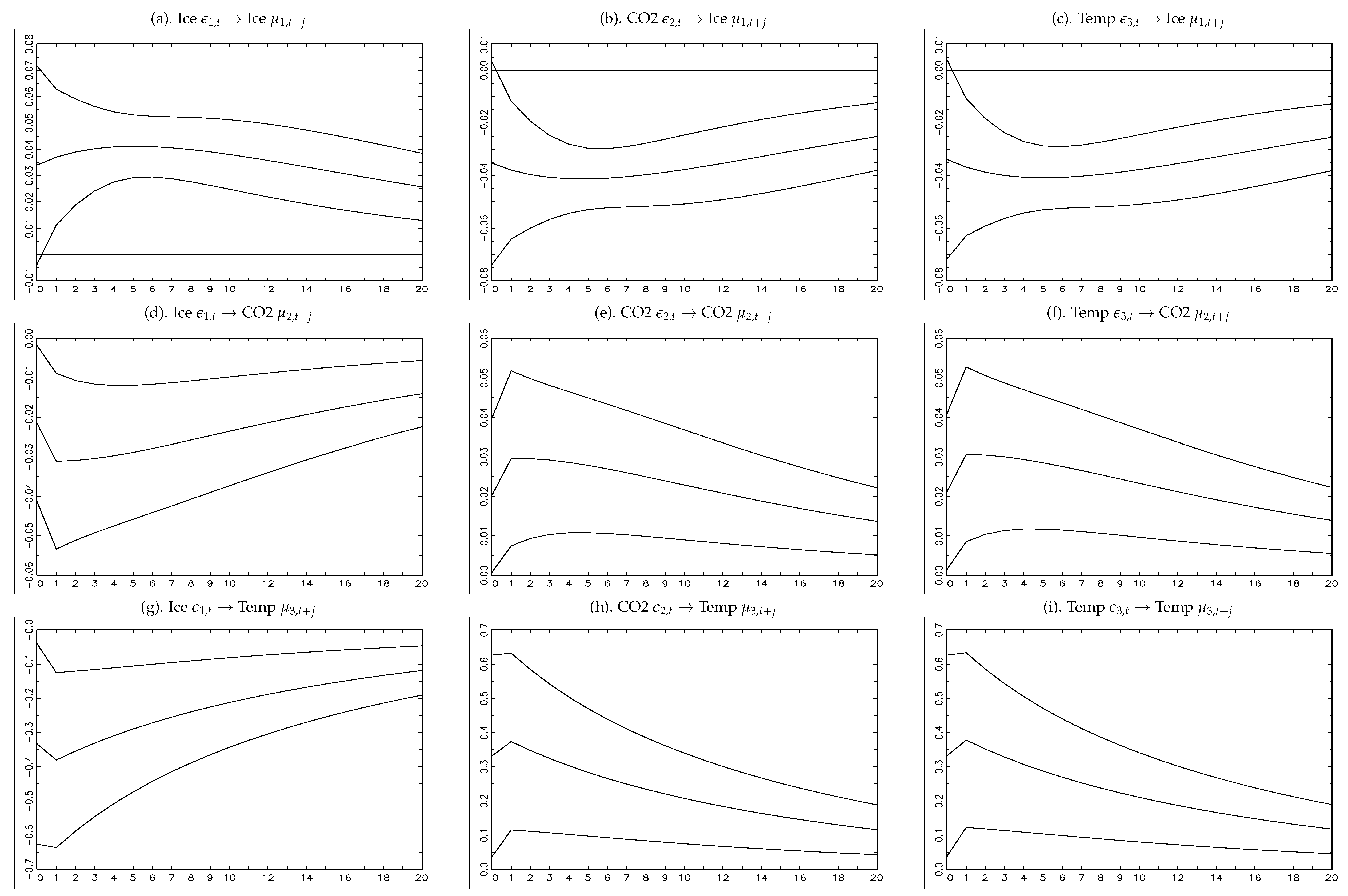
By comparing the IRF estimates of the benchmark ice-age model with those of the score-driven ice-age models, for several panels of Figure 3, Figure 4, Figure 5 and Figure 6, stronger effects are measured for the score-driven ice-age models than for the benchmark ice-age model. The strongest effects are measured for the score-driven heteroskedastic ice-age model for the t-distribution (Figure 6). We find the following differences: (i) For the benchmark ice-age model, the dynamic effects of a unit shock (i.e., measured based on the proxy) on are less than (i.e., gigatonnes of ), while for the score-driven models the same effect is stronger and it is approximately (i.e., gigatonnes of ) (Figure 3, Figure 4, Figure 5 and Figure 6, Panel (d)). (ii) For the benchmark ice-age model, the dynamic effects of a unit shock on are less than (i.e., 195 gigatonnes of ), while for the score-driven models the same effect is stronger, and it is between and (i.e., 234 and 273 gigatonnes of , respectively) (Figure 3, Figure 4, Figure 5 and Figure 6, Panel (f)). (iii) For the benchmark ice-age model, the dynamic effects of a unit shock (i.e., measured based on the proxy) on are less than °C, while for the score-driven models the same effect is stronger, reaching an estimate between and °C, respectively (Figure 3, Figure 4, Figure 5 and Figure 6, Panel (g)). (iv) For the benchmark ice-age model, the dynamic effects of a unit shock (i.e., an increase of 780 gigatonnes of in the atmosphere) on is approximately 0.35 °C, while it is above 0.40 °C for the score-driven ice-age models (Figure 3, Figure 4, Figure 5 and Figure 6, Panel (h)).
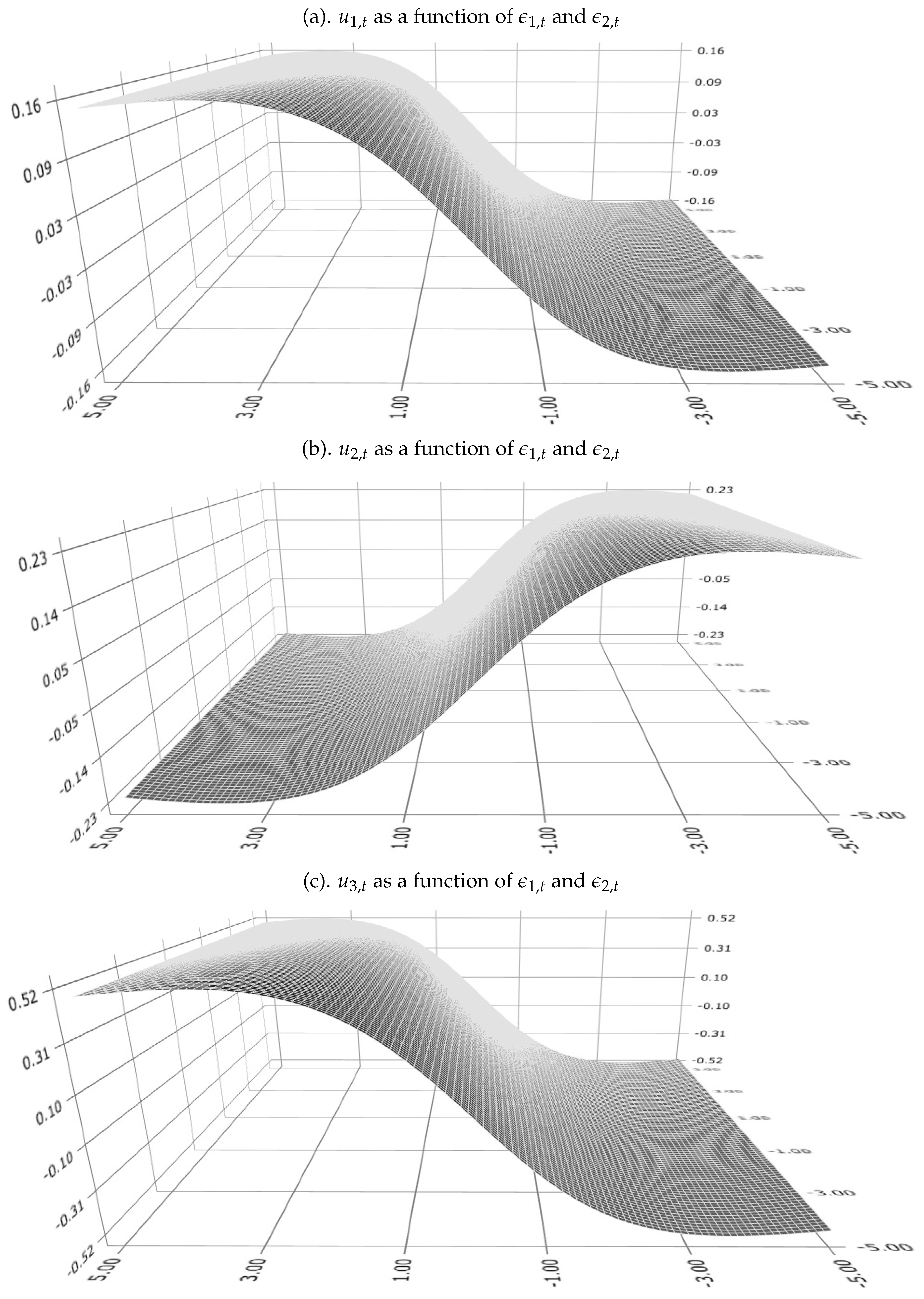
In Figure 7, we present the scaled score function as a function of the structural-form error term . The figure presents the estimates for the score-driven heteroskedastic ice-age model for the t-distribution. In the three-dimensional graphs of Figure 7, we present the elements of from Equation (30) as functions of and , where for the purpose of illustration. For the term of Equation (30), we use the unconditional mean estimate of for , which is for , respectively. The figure indicates that extreme values of are discounted by . This supports the outlier-robustness of the score-driven ice-age models of our paper.
3.3. Forecasting Results
In Table 5, the multi-step-ahead out-of-sample forecasting performances of the benchmark ice-age model and all score-driven ice-age models of the present paper are compared. The following climate variables are predicted: , , and . The estimation window is for the period of 798 thousand years ago to 101 thousand years ago (), for which humanity did not influence the Earth’s climate. The multi-step ahead forecasting window is for the last 100 thousand years (). We use two loss functions for forecasting performance evaluation: (i) mean square error (MSE), and (ii) mean absolute error (MAE). These loss functions are averaged for different periods of the last 100 thousand years (Table 5). For most of the cases, the MSE and MAE results indicate that for the periods of the last 100 thousand years to the last 30–40 thousand years, the benchmark ice-age model provides the most precise forecasts (Table 5). The results indicate for all variables that for the most recent period of the last 20–30 thousand years the score-driven homoskedastic ice-age model for the t-distribution provides the most precise forecasts (Table 5).
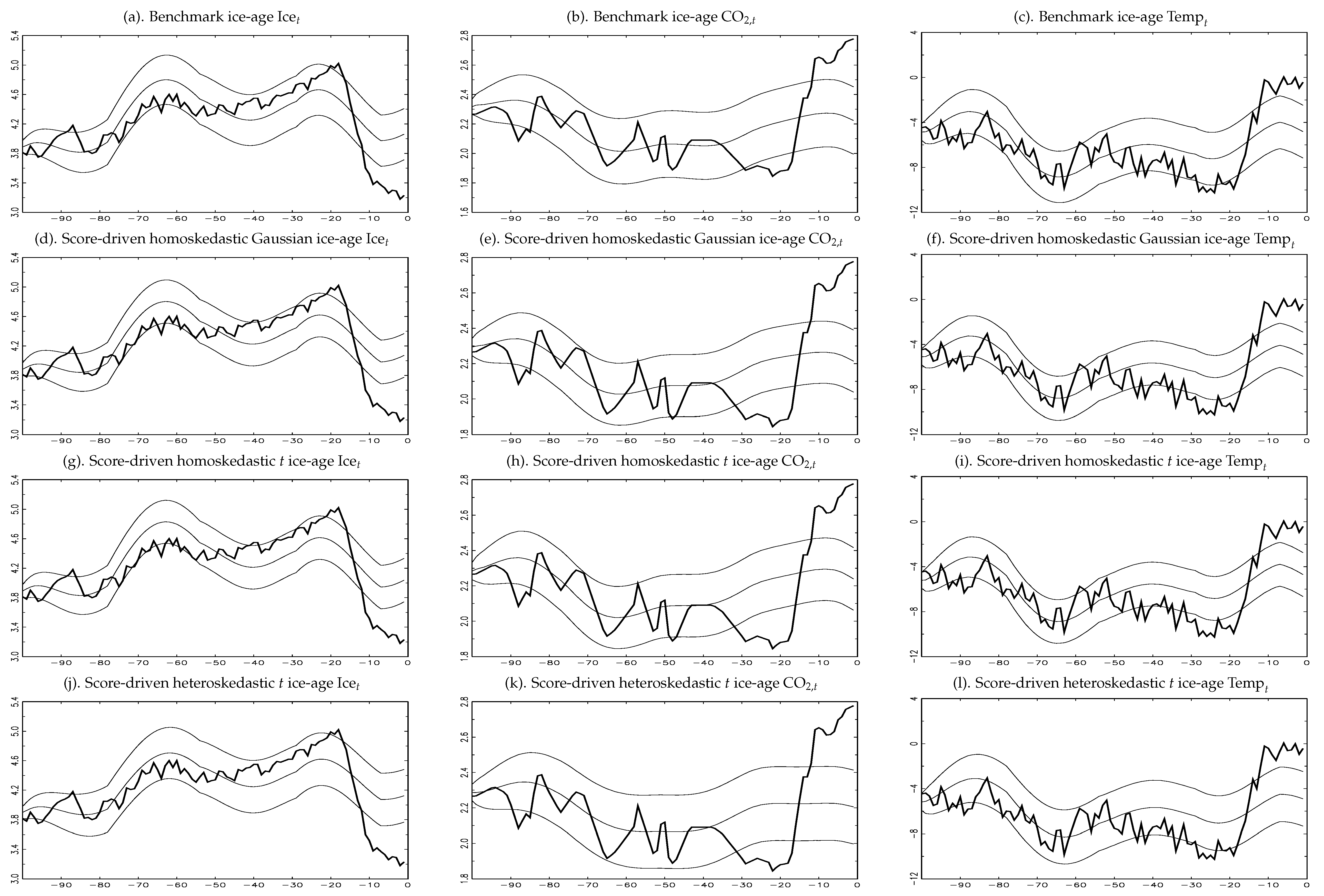
In Figure 8, the multi-step ahead out-of-sample forecasts of , , and for all ice-age models of this paper are presented. The figure includes the observed values of , , and , the forecasts of these variables, and the forecasts ± one standard deviation estimates of the forecasts. The figure shows the following results for the most recent period of the sample, when humanity impacted the Earth’s climate. For the last 10-15 thousand years of the forecasting window, the observed values of global ice volume are below the forecast interval, indicating unexpectedly low levels of global ice volume. For the same period, the observed levels of and Antarctic land surface temperature are above the forecast interval, indicating unexpectedly high levels of and Antarctic land surface temperature. These multi-step-ahead forecasting results are robust for the different econometric models (Figure 8), and are consistent with the results in the work of Castle and Hendry (2020).
The reason the observed values of the three climate variables leave the forecasting interval in Figure 8 may be due to model misspecification or the growing influence of humanity on the Earth’s climate. To study this, we repeat the multi-step ahead out-of-sample forecasting exercise for the forecasting period of 223 to 124 thousand years ago (i.e., a 100-thousand-year period), using the estimation window of the period of 798 to 224 years ago (Figure 9). For these estimation and forecasting periods, humanity did not influence the Earth’s climate. The last part of the forecasting window matches the local maximum and minimum points of the climate variables in the present time (Figure 1). We find that the observed values of the climate variables leave the forecasting interval much less in Figure 9 than in Figure 8. This result is the clearest for the most general score-driven heteroskedastic ice-age model for the t-distribution (i.e., Panels (j), (k), and (l) of Figure 8 and Figure 9).
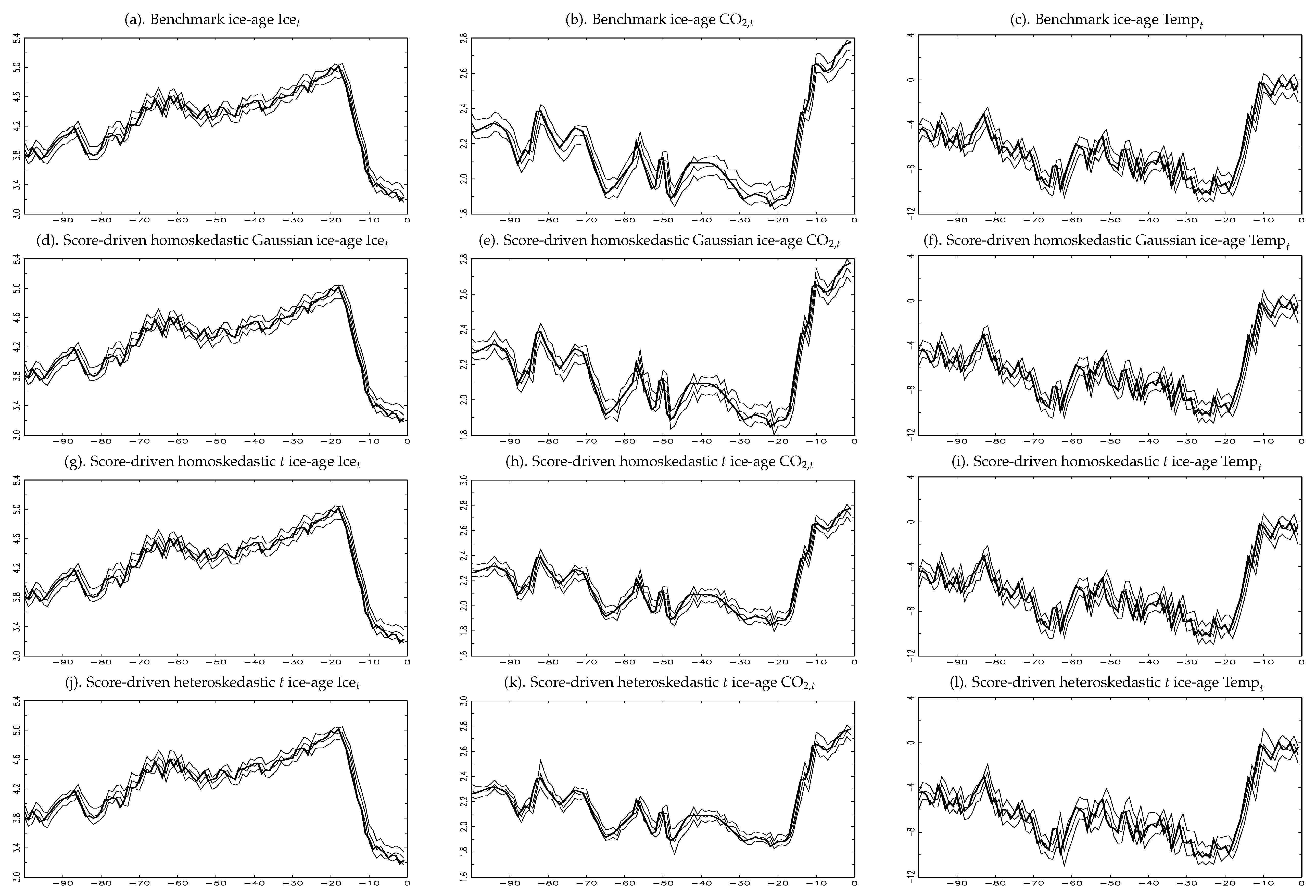
In Figure 10, the one-step ahead out-of-sample forecasts of , , and for all ice-age models of this paper are presented. We use a rolling-window approach for estimation and forecasting. The figure includes the observed values of , , and , the forecasts of these variables, and the forecasts ± one standard deviation estimates of the forecasts. For the last 10–15 thousand years, the figure shows a significant decrease in the level of global ice volume and significant increases in and Antarctic land surface temperature. For the same period, the observed values of global ice volume are unexpectedly located below the mean forecasts, and the observed values of and Antarctic land surface temperature are unexpectedly located above the mean forecasts. These forecasting results are robust for the different models.
4. Conclusions
We have used data for climate and orbital variables for the period of the last 798 thousand years, to solve the dynamic misspecification of the benchmark ice-age model. We have improved the model specification using robust score-driven models with heteroskedastic errors from the Student’s t-distribution. We have compared the statistical and forecasting performance of the benchmark ice-age model and those of our score-driven ice-age models. The statistical performance metrics and diagnostic tests have indicated that the dynamic specification of the benchmark ice-age model is improved and that the evidence of dynamic misspecification is no longer there. We have reported impulse responses for global ice volume, atmospheric , and Antarctic land surface temperature.
The forecasting results of the benchmark ice-age model are robust to the dynamic model misspecification, using data for the first 698 thousand years of the sample to forecast global ice volume, atmospheric , and Antarctic land surface temperature for the last 100 thousand years of the sample. For the last 10 to 15 thousand years when humanity influenced the Earth’s climate, we have found the following results: (i) the forecasts of global ice volume are above the observed global ice volume, (ii) the forecasts of the atmospheric level are below the observed level, and (iii) the forecasts of Antarctic land surface temperature are below the observed Antarctic land surface temperature. These results may indicate the increasing influence of humanity on the Earth’s climate, and provide a motivation to take further proactive actions to significantly reduce the greenhouse gas emissions, while respond to the most important challenge of the 21st century: global warming.
Author Contributions
Conceptualization, S.B. and A.E.; formal analysis, S.B. and A.E.; writing—original draft preparation, S.B. and A.E.; writing—review and editing, S.B. and A.E. All authors have read and agreed to the published version of the manuscript.
Funding
Blazsek acknowledges funding from Universidad Francisco Marroquín. Escribano acknowledges funding from Ministerio de Economía, Industria y Competitividad (ECO2016-00105-001 and MDM 2014-0431), Comunidad de Madrid (MadEco-CM S2015/HUM-3444), and Agencia Estatal de Investigación (2019/00419/001).
Institutional Review Board Statement
Not applicable.
Informed Consent Statement
Not applicable.
Data Availability Statement
We greatly appreciate that Jennifer L. Castle and David F. Hendry provided us with the dataset of their work (i.e., Castle and Hendry 2020, chp. 6). Data and computer codes are available from the authors of the present paper upon request.
Acknowledgments
All views expressed in this paper are strictly those of the authors and do not reflect the official views or position of any institution with which they may be affiliated or of anyone at those institutions. This paper was presented at the Annual Conference of the Hungarian Economic Society, 21–22 December 2021, Budapest. The authors are thankful for the comments and suggestions of Matthew Copley, Zsolt Darvas, David F. Hendry, and Miklós Vörös. All remaining errors are our own.
Conflicts of Interest
The authors declare no conflict of interest.
Appendix A
In all ice-age models we include exogenous orbital variables which influence the Earth’s climate in the long run, but we omit further exogenous variables that may also influence the climate. The omitted variables are: (i) the variations in the Sun’s radiation output, (ii) volcanic eruption particles in the atmosphere and ice cover, and (iii) changes in the magnetic poles. In this Appendix, we present why those variables are not included in the climate–econometric models of the present work:
(i) For the variable variations in the Sun’s radiation output, according to the literature (e.g., Feulner and Rahmstorf 2010; Jones et al. 2012; Anet et al. 2013; Meehl et al. 2013; Ineson et al. 2015; Maycock et al. 2015), the global warming of the last few decades is too large to be caused by solar activity. There are short- and long-term variations in the Sun’s radiation output. The short-term variations are the 11-year cycles (i.e., Schwabe cycles), which are part of the 22-year magnetic cycles (i.e., Hale cycles). For this paper, the long-term variations in the Sun’s radiation output, e.g., grand maximums and grand minimums which may last several centuries, and their effects on the Earth’s climate are more interesting. An example of the long-term variations is the grand minimum for the period of 1645 to 1715 approximately (i.e., the Maunder minimum), during which the solar magnetism diminished, sunspots were less frequent, and ultraviolet radiation was reduced.
The currently low level of solar activity motivated several works in the literature, to study the effects of a possible grand minimum on global surface temperatures. Feulner and Rahmstorf (2010) find that the temperature offset due to the lower level of solar activity is no more than °C for the 21st century. The same authors note that the effects of the 11-year solar cycles and the grand minimum are negligible regarding the global warming. Similar results are reported in the work of Anet et al. (2013), indicating to °C offsetting effects for the period of 2081–2100. The work of Jones et al. (2012) uses 9000-year data on the Sun’s radiation output and those authors find that the temperature offset due to the lower level of solar activity is no more than to °C for the 21st century. In the work of Meehl et al. (2013), solar irradiance is reduced by 0.25% for the period of 2020 to 2070. The results indicate that after the initial reduction of solar radiation in 2020, global surface air temperature cools by up to several tenths of a degree Centigrade compared to the reference simulation (i.e., it is not significant), and by the end of the grand solar minimum in 2070, the warming nearly catches up to the reference simulation. Meehl et al. (2013) conclude that a future grand solar minimum may slow down but not stop global warming. In the work of Ineson et al. (2015), the effects of a future scenario are investigated, for which the solar activity decreases to Maunder minimum-like conditions by 2050. The results show that the impact of that scenario on winter northern European surface temperatures over the late 21st century would not be significant. Similarly, in the work of Maycock et al. (2015), Maunder minimum-like conditions are considered for the 21st century, and the results show that the impact of such reduced solar activity is a 1.2 °C cooling at the stratopause, which is more significant than the results of other works in the literature, but it is much lower than projected temperature increases due to global warming.
With respect to the observation period of solar activity, the short-term solar cycles have been observed since 1610 (i.e., the first telescopic observations). Moreover, we also refer to the proxy records of solar activity in the work of Steinhilber et al. (2008), which creates a time series of solar modulation potential for the last 9300 years, that, to the best of our knowledge, is the longest available observation period of solar activity in the literature.
We omit the variable on solar activity from the econometric models of this paper, because the global warming of the last few decades is too large to be caused by solar activity, and we do not have data on solar activity for the full sample period of the last 798 thousand years.
(ii) The impact of volcanic eruptions on the climate depends on the location of the volcano. Eruptions in the tropics influence the climate more than eruptions at mid or high latitudes which only influence the hemisphere they are within. The gases and dust particles entering the Earth’s atmosphere from volcanic eruptions influence the climate. The dust particles cool the planet by shading incoming solar radiation, which can last from months to years. Particularly effective cooling particles emitted during volcanic eruptions are the sulfuric gases, which move into the stratosphere and combining with water form sulfate aerosols that reflect the incoming solar radiation. The sulfate aerosols may stay in the stratosphere for 3–4 years. The sulfate aerosol absorption heats the stratosphere, but a reduction of downward radiation at the tropopause cools the troposphere and the underlying surface (Stenchikov et al. 1998; Kirchner et al. 1999). Volcanic eruptions also influence global warming when greenhouse gases, such as water vapor and are released into the atmosphere. The cooling effects of dust and sulfate aerosol particles, and the relatively small volume of heating greenhouse gases emitted by volcanic eruptions (compared to the volume of greenhouse gases in the Earth’s atmosphere) do not significantly influence the Earth’s climate in the long term. Moreover, data on volcanic eruptions for the period of the last 798 thousand years of this paper are not available. Hence, the omission of the variable volcanic eruption particles in the atmosphere and ice cover in the econometric models.
(iii) According to NASA (2021), changes in the magnetic poles do not influence the Earth’s climate, because there is little scientific evidence of any significant links between Earth’s drifting magnetic poles and climate. The changes in the magnetic poles can be classified into three categories: First, shifts in magnetic pole locations (with a speed of approximately 16 to 55 kilometers per year). Second, Earth’s magnetic north and south poles swap locations (the frequency is variable, but on average it takes place in every 300 thousand years, with the last one taking place about 780 thousand years ago). Third, geomagnetic excursions which are shorter-lived but significant changes in the magnetic field’s intensity with duration of a few centuries to a few tens of thousands of years (the last major excursion, named the Laschamps event, took place about 41,500 years ago, when the magnetic field weakened significantly, the poles reversed, and flipped back about 500 years later). The changes in the magnetic poles does not influence the Earth’s climate, at least because of two reasons NASA (2021): First, there is insufficient energy in the Earth’s upper atmosphere (where electromagnetic currents exist), to influence the Earth’s climate. Second, there is no known physical mechanism capable of connecting weather conditions at the Earth’s surface with electromagnetic currents in space. Hence, the omission of changes in the magnetic poles.
References
- Anet, Julien G., E. V. Rozanov, Stefan Muthers, T. Peter, Stefan Brönnimann, F. Arfeuille, J. Beer, A. I. Shapiro, C. C. Raible, F. Steinhilber, and et al. 2013. Impact of a potential 21st century “grand solar minimum” on surface temperatures and stratospheric ozone. Geophysical Research Letters 40: 4420–25. [Google Scholar] [CrossRef] [Green Version]
- Archer, David, Pamela Martin, Bruce Buffett, Victor Brovkin, Stefan Rahmstorf, and Andrey Ganopolski. 2004. The importance of ocean temperature to global biogeochemistry. Earth and Planetary Science Letters 222: 333–48. [Google Scholar] [CrossRef]
- Blasques, Francisco, Janneke van Brummelen, Siem Jan Koopman, and Andre Lucas. 2021. Maximum likelihood estimation for score-driven models. Journal of Econometrics. [Google Scholar] [CrossRef]
- Blasques, Francisco, Siem Jan Koopman, and Andre Lucas. 2015. Information-theoretic optimality of observation-driven time series models for continuous responses. Biometrika 102: 325–43. [Google Scholar] [CrossRef]
- Blazsek, Szabolcs, Alvaro Escribano, and Adrian Licht. 2020. Identification of seasonal effects in impulse responses using score-driven multivariate location models. Journal of Econometric Methods 10: 53–66. [Google Scholar] [CrossRef]
- Blazsek, Szabolcs, Alvaro Escribano, and Adrian Licht. 2021a. Co-integration with score-driven models: An application to US real GDP growth, US inflation rate, and effective federal funds rate. Macroeconomic Dynamics, 1–21. [Google Scholar] [CrossRef]
- Blazsek, Szabolcs, Alvaro Escribano, and Adrian Licht. 2021b. Multivariate Markov-switching score-driven models: An application to the global crude oil market. Studies in Nonlinear Dynamics & Econometrics. [Google Scholar] [CrossRef]
- Bollerslev, Tim. 1986. Generalized autoregressive conditional heteroskedasticity. Journal of Econometrics 31: 307–27. [Google Scholar] [CrossRef] [Green Version]
- Box, George E. P., and Gwilym M. Jenkins. 1970. Time Series Analysis, Forecasting and Control. San Francisco: Holden-Day. [Google Scholar]
- Bronselaer, Ben, Michael Winton, Stephen M. Griffies, William J. Hurlin, Keith B. Rodgers, Olga V. Sergienko, Roland J. Stouffer, and Joellen L. Russell. 2018. Change in future climate due to Antarctic meltwater. Nature 564: 53–58. [Google Scholar] [CrossRef]
- Castle, Jennifer, and David F. Hendry. 2020. Climate econometrics: An overview. Foundations and Trends in Econometrics 10: 145–322. [Google Scholar] [CrossRef]
- Cox, David R. 1981. Statistical analysis of time series: Some recent developments. Scandinavian Journal of Statistics 8: 93–115. [Google Scholar]
- Creal, Drew, Siem Jan Koopman, and Andre Lucas. 2008. A General Framework for Observation Driven Time-Varying Parameter Models. Tinbergen Institute Discussion Paper 08-108/4. Available online: https://www.tinbergen.nl/discussion-paper/2649/08-108-4-a-general-framework-for-observation-driven-timevarying-parameter-models (accessed on 25 December 2021).
- Creal, Drew, Siem Jan Koopman, and Andre Lucas. 2011. A dynamic multivariate heavy-tailed model for time-varying volatilities and correlations. Journal of Business & Economic Statistics 29: 552–63. [Google Scholar] [CrossRef] [Green Version]
- Creal, Drew, Siem Jan Koopman, and Andre Lucas. 2013. Generalized autoregressive score models with applications. Journal of Applied Econometrics 28: 777–95. [Google Scholar] [CrossRef] [Green Version]
- Engle, Robert. 2002. Dynamic conditional correlation: A simple class of multivariate generalized autoregressive conditional heteroskedasticity models. Journal of Business & Economic Statistics 20: 339–51. [Google Scholar] [CrossRef]
- Feulner, Georg, and Stefan Rahmstorf. 2010. On the effect of a new grand minimum of solar activity on the future climate on Earth. Geophysical Research Letters 37. [Google Scholar] [CrossRef] [Green Version]
- Harvey, Andrew C. 2013. Dynamic Models for Volatility and Heavy Tails: With Applications to Financial and Economic Time Series. Econometric Society Monographs. Cambridge: Cambridge University Press. [Google Scholar]
- Harvey, Andrew C., and Tirthankar Chakravarty. 2008. Beta-t-(E)GARCH. Cambridge Working Papers in Economics 0840. Cambridge: Faculty of Economics, University of Cambridge, Available online: http://www.econ.cam.ac.uk/research/repec/cam/pdf/cwpe0840.pdf (accessed on 25 December 2021).
- Ineson, Sarah, Amanda C. Maycock, Lesley J. Gray, Adam A. Scaife, Nick J. Dunstone, Jerald W. Harder, Jeff R. Knight, Mike Lockwood, James C. Manners, and Richard A. Wood. 2015. Regional climate impacts of a possible future grand solar minimum. Nature Communications 6: 443. [Google Scholar] [CrossRef]
- Intergovernmental Panel on Climate Change. 2021. Sixth Assessment Report. Available online: https://www.ipcc.ch/report/ar6/wg1/#SPM (accessed on 25 December 2021).
- Jones, Gareth S., Mike Lockwood, and Peter A. Stott. 2012. What influence will future solar activity changes over the 21st century have on projected global near-surface temperature changes? Journal of Geographical Research 117. [Google Scholar] [CrossRef]
- Jouzel, J., V. Masson-Delmotte, O. Cattani, G. Dreyfus, S. Falourd, and G. E. Hoffmann. 2007. Orbital and millennial Antarctic climate variability over the past 800,000 years. Science 317: 793–97. [Google Scholar] [CrossRef] [Green Version]
- Kibria, B. M. Golam, and Anwar H. Joarder. 2006. A short review of multivariate t-distribution. Journal of Statistical Research 40: 59–72. [Google Scholar]
- Kirchner, Ingo, Georgiy L. Stenchikov, Hans-F. Graf, Alan Robock, and Juan Carlos Antuna. 1999. Climate model simulation of winter warming and summer cooling following the 1991 Mount Pinatubo volcanic eruption. Journal of Geophysical Research 104: 19039–55. [Google Scholar] [CrossRef]
- Lisiecki, Lorraine E., and Maureen E. Raymo. 2005. A pliocene-pleistocene stack of 57 globally distributed Benthic δ18O records. Paleoceanography 20. [Google Scholar] [CrossRef] [Green Version]
- Ljung, Greta M., and George E. P. Box. 1978. On a measure of lack of fit in time-series models. Biometrika 65: 297–303. [Google Scholar] [CrossRef]
- Lüthi, Dieter, Marthine Le Floch, Bernhard Bereiter, Thomas Blunier, Jean-Marc Barnola, Urs Steigenhaler, Dominique Raynaud, Jean Jouzel, Hubertus Fischer, Kenji Kawamura, and et al. 2008. High-resolution carbon dioxide concentration record 650,000–800,000 years before present. Nature 453. [Google Scholar] [CrossRef]
- Lütkepohl, Helmut. 2005. New Introduction to Multivariate Time Series Analysis. Berlin and Heidelberg: Springer. [Google Scholar]
- Maycock, A. C., S. Ineson, L. J. Gray, A. A. Scaife, J. A. Anstey, M. Lockwood, N. Butchart, S. C. Hardiman, D. M. Mitchell, and S. M. Osprey. 2015. Possible impacts of a future grand solar minimum on climate: Stratospheric and global circulation changes. JGR Atmospheres 120: 9043–58. [Google Scholar] [CrossRef] [Green Version]
- Meehl, Gerald A., Julie M. Arblaster, and Daniel R. Marsh. 2013. Could a future “Grand Solar Minimum” like the Maunder Minimum stop global warming? Geographical Research Letters 40: 1789–93. [Google Scholar] [CrossRef]
- NASA. 2021. Flip flop: Why Variations in Earth’s Magnetic Field Aren’t Causing Today’S Climate Change. Available online: https://climate.nasa.gov/ask-nasa-climate/3104/flip-flop-why-variations-in-earths-magnetic-field-arent-causing-todays-climate-change/ (accessed on 25 December 2021).
- Paillard, Didier, Laurent D. Labeyrie, and Pascal Yiou. 1996. Macintosh program performs time-series analysis. Eos Transactions AGU 77: 379–79. [Google Scholar] [CrossRef]
- Qin, Zhao, and Markus J. Buehler. 2012. Carbon dioxide enhances fragility of ice crystals. Journal of Physics D: Applied Physics 45. [Google Scholar] [CrossRef]
- Rubio-Ramirez, Juan F., Daniel Waggoner, and Tao Zha. 2010. Structural vector autoregressions: Theory for identification and algorithms for inference. Review of Economic Studies 77: 665–96. [Google Scholar] [CrossRef] [Green Version]
- Ruddiman, William. 2005. Plows, Plagues and Petroleum: How Humans Took Control of the Climate. Princeton: Princeton University Press. [Google Scholar]
- Steinhilber, F., J. A. Abreu, and J. Beer. 2008. Solar modulation during the Holocene. Astrophysics and Space Sciences Transactions 4: 1–6. [Google Scholar] [CrossRef] [Green Version]
- Stenchikov, Georgiy L., Ingo Kirchner, Alan Robock, Hans-F. Graf, Juan Carlos Antuna, R. G. Grainger, Alyn Lambert, and Larry Thomason. 1998. Radiative Forcing from the 1991 Mount Pinatubo volcanic eruption. Journal of Geophysical Research 103: 13837–57. [Google Scholar] [CrossRef] [Green Version]
- Tiao, George C., and Ruey S. Tsay. 1989. Model specification in multivariate time series. Journal of the Royal Statistical Society 51: 157–213. [Google Scholar] [CrossRef]
- Wadham, J. L., J. R. Hawkings, L. Tarasov, L. J. Gregoire, R. G. M. Spencer, M. Gutjahr, A. Ridgwell, and K. E. Kohfeld. 2019. Ice sheets matter for the global carbon cycle. Nature Communications 10: 3567. [Google Scholar] [CrossRef] [PubMed] [Green Version]
- White, Halbert. 2001. Asymptotic Theory for Econometricians. revised edition. San Diego: Academic Press. [Google Scholar]
Figure 1.
Evolution of , , and from 798 thousand years ago to 1 thousand years ago.

Figure 2.
Evolution of , , and from 798 thousand years ago to 1 thousand years ago.

Figure 3.
IRFs up to 20 lags for the benchmark ice-age model. Notes: The confidence interval is mean ± one standard deviation that is estimated for 2302 out of the 3 million simulations under the restrictions of Table 1. Ice uses the proxy; 1 is 780 gigatonnes; 1 Temp is 1 °C.
Figure 3.
IRFs up to 20 lags for the benchmark ice-age model. Notes: The confidence interval is mean ± one standard deviation that is estimated for 2302 out of the 3 million simulations under the restrictions of Table 1. Ice uses the proxy; 1 is 780 gigatonnes; 1 Temp is 1 °C.

Figure 4.
IRFs up to 20 lags for the score-driven ice-age model for the normal distribution. Notes: The confidence interval is mean ± one standard deviation that is estimated for 1771 out of the 3 million simulations under the restrictions of Table 1. Ice uses the proxy; 1 is 780 gigatonnes; 1 Temp is 1 °C.

Figure 5.
IRFs up to 20 lags for the score-driven homoskedastic ice-age model for the t-distribution. Notes: The confidence interval is mean ± one standard deviation that is estimated for 2289 out of the 3 million simulations under the restrictions of Table 1. Ice uses the proxy; 1 is 780 gigatonnes; 1 Temp is 1 °C.

Figure 6.
IRFs up to 20 lags for the score-driven heteroskedastic ice-age model for the t-distribution. Notes: The confidence interval is mean ± one standard deviation that is estimated for 1698 out of the 3 million simulations under the restrictions of Table 1. Ice uses the proxy; 1 is 780 gigatonnes; 1 Temp is 1 °C.

Figure 7.
Robustness of the scaled score function to extreme values. Note: is assumed for this figure.
Figure 7.
Robustness of the scaled score function to extreme values. Note: is assumed for this figure.

Figure 8.
Multi-step ahead out-of-sample forecasts for the period of the last 100 thousand years. Notes: The confidence interval is mean ± one standard deviation. The true values are indicated by thick lines.
Figure 8.
Multi-step ahead out-of-sample forecasts for the period of the last 100 thousand years. Notes: The confidence interval is mean ± one standard deviation. The true values are indicated by thick lines.

Figure 9.
Multi-step ahead out-of-sample forecasts for the period of 223 to 124 thousand years ago. Notes: The confidence interval is mean ± one standard deviation. The true values are indicated by thick lines.
Figure 9.
Multi-step ahead out-of-sample forecasts for the period of 223 to 124 thousand years ago. Notes: The confidence interval is mean ± one standard deviation. The true values are indicated by thick lines.

Figure 10.
One-step ahead out-of-sample forecasts for the last 100 thousand years. Notes: The confidence interval is mean ± one standard deviation. The true values are indicated by thick lines.
Figure 10.
One-step ahead out-of-sample forecasts for the last 100 thousand years. Notes: The confidence interval is mean ± one standard deviation. The true values are indicated by thick lines.


Table 1.
Sign restrictions on contemporaneous impact responses.
| Shock | Shock | Shock | |
|---|---|---|---|
| + | − | − | |
| − | + | + | |
| − | + | + |
Table 2.
Descriptive statistics.
| (a) Dependent Variables | |||
|---|---|---|---|
| Variable | Ice volume | Atmospheric | Antarctic-based land surface temperature |
| Start date | 798 thousand years ago | 798 thousand years ago | 798 thousand years ago |
| End date | 1 thousand years ago | 1 thousand years ago | 1 thousand years ago |
| Data frequency | 1 thousand years | 1 thousand years | 1 thousand years |
| Measurement | Based on the proxy | 1 unit = 780 gigatonnes of | 1 unit = 1 Celsius degree |
| Data source | Lisiecki and Raymo (2005) | Lüthi et al. (2008) | Jouzel et al. (2007) |
| Sample size | 798 | 798 | 798 |
| Minimum | |||
| Maximum | |||
| Mean | |||
| Standard deviation | |||
| (b) Explanatory Variables | |||
| Variable | Eccentricity of the Earth’s orbit | Obliquity | Precession of the equinox |
| Start date | 798 thousand years ago | 798 thousand years ago | 798 thousand years ago |
| End date | 1 thousand years ago | 1 thousand years ago | 1 thousand years ago |
| Data frequency | 1 thousand years | 1 thousand years | 1 thousand years |
| Measurement | Periodicity deriving from the | Periodicity deriving from the | Periodicity deriving from the |
| changing non-circularity of the Earth’s orbit | changes in the tilt of the Earth’s rotational axis | precession of the equinox | |
| (zero denotes circularity). | relative to the ecliptic (1 unit = 10 degrees). | (1 unit = 1 degree). | |
| Data source | Paillard et al. (1996) | Paillard et al. (1996) | Paillard et al. (1996) |
| Sample size | 798 | 798 | 798 |
| Minimum | |||
| Maximum | |||
| Mean | |||
| Standard deviation |
Table 3.
In-sample ML parameter estimates.
| Benchmark | Score-Driven Homoskedastic | Score-Driven Homoskedastic | Score-Driven Heteroskedastic | ||||||
|---|---|---|---|---|---|---|---|---|---|
| Ice-Age Model | Gaussian Ice-Age Model | t Ice-Age Model | t Ice-Age Model | ||||||
| *** | *** | *** | *** | *** | |||||
| *** | *** | *** | *** | *** | |||||
| *** | *** | ||||||||
| *** | *** | *** | *** | *** | |||||
| *** | *** | *** | *** | *** | |||||
| *** | *** | *** | *** | *** | |||||
| *** | *** | *** | *** | *** | |||||
| *** | *** | ||||||||
| *** | *** | *** | *** | *** | |||||
| *** | *** | *** | *** | *** | |||||
| *** | *** | *** | *** | ||||||
| *** | *** | *** | *** | ||||||
| *** | *** | *** | *** | ||||||
| *** | *** | *** | *** | ||||||
| *** | *** | *** | *** | ||||||
| *** | *** | *** | *** | ||||||
| *** | *** | *** | *** | ||||||
| *** | *** | *** | *** | ||||||
| *** | *** | *** | *** | ||||||
| *** | *** | *** | *** | ||||||
| *** | *** | *** | *** | ||||||
| *** | *** | *** | *** | ||||||
| ** | ** | *** | *** | ||||||
| *** | *** | *** | *** | ||||||
| NA | *** | *** | *** | ||||||
| NA | *** | *** | *** | ||||||
| NA | *** | *** | *** | ||||||
| NA | *** | *** | *** | ||||||
| NA | *** | *** | *** | ||||||
| NA | *** | *** | *** | ||||||
| *** | *** | *** | NA | ||||||
| *** | *** | *** | *** | ||||||
| *** | *** | *** | NA | ||||||
| *** | *** | *** | *** | ||||||
| *** | *** | *** | *** | ||||||
| *** | *** | *** | NA | ||||||
| NA | NA | *** | *** | ||||||
Notes: Not available (NA). Standard errors are reported in parentheses. ***, **, *, and + indicate significance at the 1%, 5%, 10%, and 15% levels, respectively.
Table 4.
Model performance and diagnostics for in-sample estimates.
| Benchmark | Score-Driven Homoskedastic | Score-Driven Homoskedastic | Score-Driven Heteroskedastic | |
|---|---|---|---|---|
| Ice-Age Model | Gaussian Ice-Age Model | t Ice-Age Model | t Ice-Age Model | |
| LL | ||||
| AIC | ||||
| BIC | ||||
| HQC | ||||
| NA | NA | NA | ||
| NA | NA | NA | ||
| NA | NA | NA | ||
| LB (p-value) | ||||
| LB (p-value) | *** | |||
| LB (p-value) | ** | |||
| LB (p-value) | ||||
| LB (p-value) | *** | |||
| LB (p-value) | ** | ** | ** | |
| LB (p-value) | NA | NA | ||
| LB (p-value) | NA | NA | ||
| LB (p-value) | NA | NA | ||
| LB (p-value) | NA | NA | NA | |
| LB (p-value) | NA | NA | NA | |
| LB (p-value) | NA | NA | NA |
Notes: Not available (NA); log-likelihood (LL); Akaike information criterion (AIC); Bayesian information criterion (BIC); Hannan–Quinn criterion (HQC); Ljung–Box (LB). is the maximum modulus of eigenvalues of the matrix , for which indicates covariance stationarity of the location filter. for , for which for indicates covariance stationarity of the scale filter. The lag-order for the LB test is . *** and ** indicate significance at the 1% and 5% levels, respectively.
Table 5.
Multi-step ahead forecasts for the last 100 thousand years.
| Score-Driven | Score-Driven | |||||||
|---|---|---|---|---|---|---|---|---|
| Homoskedastic | Score-Driven | Score-Driven | Homoskedastic | Score-Driven | Score-Driven | |||
| Benchmark | Gaussian | Homoskedastic | Heteroskedastic | Benchmark | Gaussian | Homoskedastic | Heteroskedastic | |
| Ice-Age Model | Ice-Age Model | t Ice-Age Model | t Ice-Age Model | Ice-Age Model | Ice-Age Model | t Ice-Age Model | t Ice-Age Model | |
| MSE | MSE | MSE | MSE | MAE | MAE | MAE | MAE | |
| last 100,000 years | ||||||||
| last 90,000 years | ||||||||
| last 80,000 years | ||||||||
| last 70,000 years | ||||||||
| last 60,000 years | ||||||||
| last 50,000 years | ||||||||
| last 40,000 years | ||||||||
| last 30,000 years | ||||||||
| last 20,000 years | ||||||||
| last 10,000 years | ||||||||
| MSE | MSE | MSE | MSE | MAE | MAE | MAE | MAE | |
| last 100,000 years | ||||||||
| last 90,000 years | ||||||||
| last 80,000 years | ||||||||
| last 70,000 years | ||||||||
| last 60,000 years | ||||||||
| last 50,000 years | ||||||||
| last 40,000 years | ||||||||
| last 30,000 years | ||||||||
| last 20,000 years | ||||||||
| last 10,000 years |
Notes: Mean square error (MSE); mean absolute error (MAE). The lowest loss function values are indicated by bold numbers.
Publisher’s Note: MDPI stays neutral with regard to jurisdictional claims in published maps and institutional affiliations. |
© 2022 by the authors. Licensee MDPI, Basel, Switzerland. This article is an open access article distributed under the terms and conditions of the Creative Commons Attribution (CC BY) license (https://creativecommons.org/licenses/by/4.0/).
Share and Cite
MDPI and ACS Style
Blazsek, S.; Escribano, A. Robust Estimation and Forecasting of Climate Change Using Score-Driven Ice-Age Models. Econometrics 2022, 10, 9. https://0-doi-org.brum.beds.ac.uk/10.3390/econometrics10010009
AMA Style
Blazsek S, Escribano A. Robust Estimation and Forecasting of Climate Change Using Score-Driven Ice-Age Models. Econometrics. 2022; 10(1):9. https://0-doi-org.brum.beds.ac.uk/10.3390/econometrics10010009
Chicago/Turabian StyleBlazsek, Szabolcs, and Alvaro Escribano. 2022. "Robust Estimation and Forecasting of Climate Change Using Score-Driven Ice-Age Models" Econometrics 10, no. 1: 9. https://0-doi-org.brum.beds.ac.uk/10.3390/econometrics10010009
Note that from the first issue of 2016, this journal uses article numbers instead of page numbers. See further details here.