Article

Spatiotemporal Analysis of Urban Heat Islands in Relation to Urban Development, in the Vicinity of the Atacama Desert

1
Department of Architecture, Jorge Basadre Grohmann National University, Tacna 23000, Peru
2
Department of Civil Engineering, Jorge Basadre Grohmann National University, Tacna 23000, Peru
3
RED YAKU E.I.R.L., Lima 15012, Peru
*
Author to whom correspondence should be addressed.
Submission received: 10 May 2022 / Revised: 13 June 2022 / Accepted: 15 June 2022 / Published: 16 June 2022

Abstract

:
Near the Atacama Desert, Tacna city in Peru is among the largest arid cities with constant urban development, thus understanding of the urban surface thermal pattern is needed. We propose a comprehensive study of the urban heat island phenomenon, with the objective of (1) determining the spatial and temporal variations of the urban heat islands (UHIs), in the period 1985 to 2020; (2) analyzing the relationship between the UHI and influencing factors such as vegetation, urban area, and population, using indices calculated with satellite images. The Google Earth Engine repository was used to evaluate the corrected images from the years 1985 to 2020. The coincidence between the normalized difference vegetation index (NDVI) and normalized difference built-up index (NDBI) was good, negative between NDVI and the land surface temperature (LST), attributable to dense vegetation, and negative and very high (−0.81) between NDBI and NDVI, as massive urbanization leads to the reduction in the vegetal surface. The NDBI has a high impact on the LST; a coefficient of connections is recorded as 0.46. Tacna is a very arid region, and an increase in the time of the LST occurred with the increase in industrialization and urbanization. The land use/cover change (LUCC) evidences change in the climate in the city of Tacna; temperatures of 24.2 °C to 44.2 °C are observed in the built-up areas. In vegetated areas, the temperature remains below 24 °C, which is associated with a high rate of potential evapotranspiration. Thus, this study shows that variations in urban form and growth have produced the development of intraurban surface thermal patterns.

1. Introduction

With rapid urbanization, population growth, and anthropogenic activities, an increasing number of major cities around the world are facing severe urban heat islands (UHIs) [1]. Urban heat island (UHI) is one of the clearest examples of inadvertent climate modification due to humans [2]. Changes in the urban landscape resulting from rapid urbanization and climate change have the potential to increase the land surface temperature (LST) and the incidence of UHIs [3,4]. In recent decades, climate change has gained relevance and is becoming crucial to assess the performance of buildings [5]. Political and technological responses to rising UHI temperatures are discussed in several studies [6]; however, little is known about their interaction [7].
Extreme heat events in urban centers in combination with air pollution pose a serious risk to human health [8]. Cities around the world are facing various challenges related to urbanization and climate change [9]. In this sense, cities are increasingly adopting potentially sustainable climate plans [10]. The conditioning factors of the context and typology of trees and their characteristics directly influence the effects of cooling in the city [11].
The UHI effect is a phenomenon of heat accumulation in the urban area due to buildings and human activities [12]. It is recognized as the most evident characteristic of the urban climate. The LST is one of the crucial parameters in the physical processes of the Earth [13], but the acquisition of LST images with high spatial and temporal resolution is currently difficult due to the technical restriction of thermal infrared sensors of satellites [14]. It is possible to estimate the LST from Landsat 5, 7, and 8 thermal infrared sensors, using different sources of surface emissivity [15,16].
UHIs have been investigated in many regions of the world, but little attention has been paid in South America [17]. In South America (Brazil), it was determined that morphology directly interferes with the local microclimate; in the case of tropical cities, the increase in temperature and the change in the dynamics of the winds can cause heat islands [18]. Vertical growth should eventually be used, combined with passive strategies to cool the city, implementing the use of natural ventilation when available on the South American coast [19]. Use of private vehicles should be reduced by planning a better public transport system and a different distribution of land use patterns, seeking mixed land use, in order to reduce the distances between homes, commercial premises, and others [17,18].
Urban growth is related to the change in land use, as a response to migratory issues, but mainly to the increase in population [20] and other factors such as seismogenic characteristics [21]; the relationship between change in use, land cover, and population growth will allow us to understand various urban environmental problems [4,22].
There is a positive correlation between LST and the normalized difference built-up index (NDBI), while the normal difference vegetation index (NDVI) indicates a negative correlation with LST [23,24].
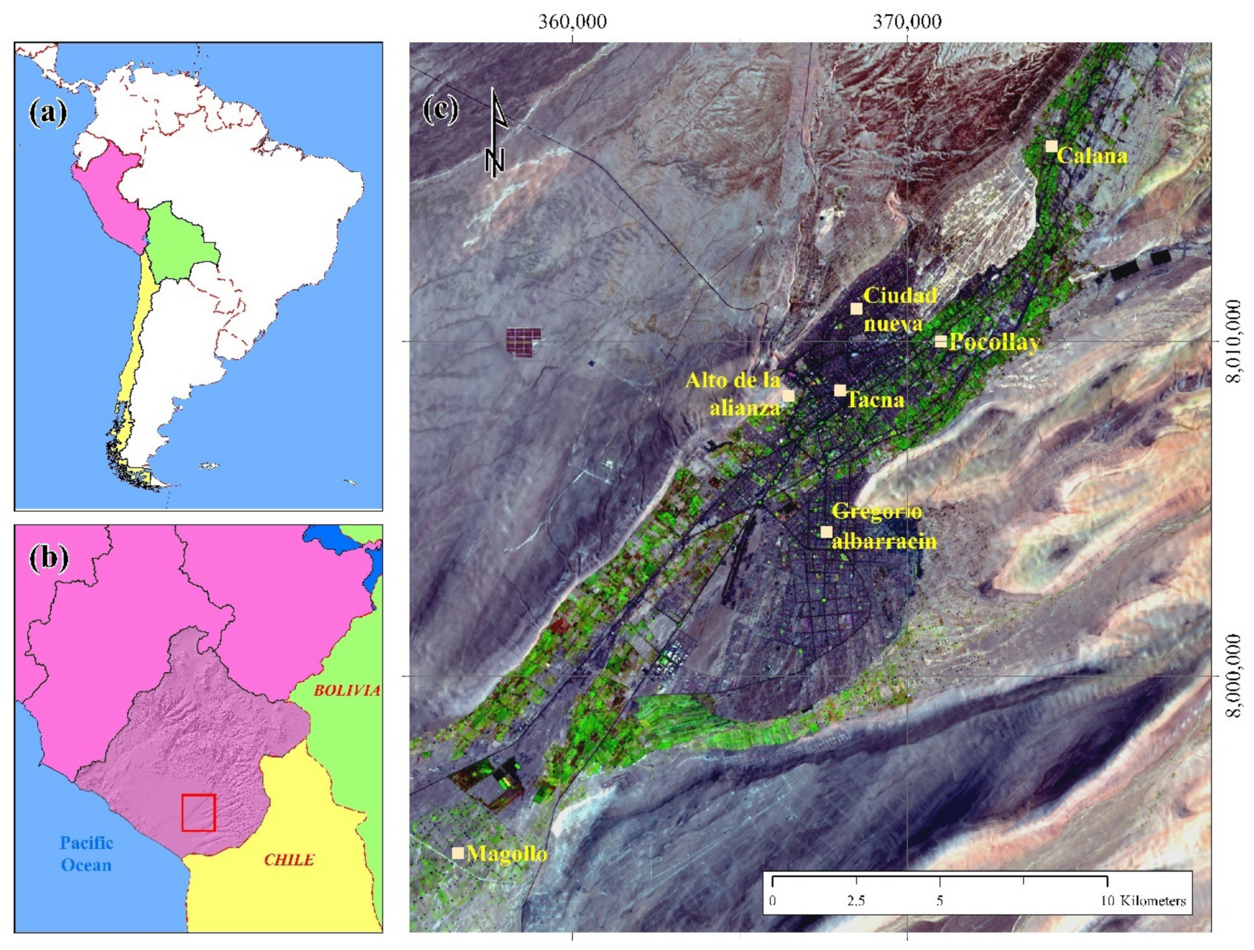
This work proposes a comprehensive study of the urban heat island phenomenon in the city of Tacna, Peru, located at the head of the Atacama Desert, with the objective of determining the spatial and temporal variations of the UHI, in the period 1985 to 2020; and analyzing the relationship between the UHI and influencing factors such as vegetation, urban area, and population, using indexes calculated from satellite images.
The study of UHIs and their spatiotemporal variability, in correlation with vegetation indexes, is a useful urban planning tool for policy makers, planners, and urban investors, mitigating the accelerated degradation of the environment and improving the quality of life of its inhabitants.

2. Materials and Methods

2.1. Study Area

The study area is located in the Tacna region (Figure 1), located at the head of the Atacama Desert, in the extreme south of Peru and north of Chile (17°55.90′–18°8.60′ South Latitude, 70°12.86′–70°19.56′ West Longitude of Greenwich). The city, according to the 2017 Population and Housing Census, has 329,332 inhabitants that constitute 1.1% of the Peruvian population and an annual average growth rate of 1.3% (calculated from 2007 to 2017). The regional economy grows at an average of 4.8% per year compared to the national growth of 2.4%, highlighting mining as the main economic activity with a 50.9% share. In this region, the availability of water to meet the demands of the population and for agricultural use is increasingly scarce [24,25,26,27,28,29,30]. This region is located in one of the main deserts in the world [30]; it has a hyperarid climate and is attributed to its subtropical location [31,32]. The climate is also defined by its geographical location, where two thirds of its territory is in the coastal region, which is characterized by a dry climate with temperature variations between 12 °C and 30 °C and with occasional and scarce rains [33,34]. The demographic growth has modified land use and surface coverage; within this context, a polygon has been determined, currently made up of the districts of Tacna, Alto de la Alianza, Calana, Ciudad Nueva, Pocollay, Gregorio Albarracín, and La Yarada (see Figure 1).

2.2. Obtaining and Processing Satellite Images

It is possible to use multispectral images from Enhanced Thematic Mapper Plus (ETM) and Operational Land Imager (OLI) sensors. They have a spatial resolution of 30 m for visible and infrared shortwave spectra, and a temporal resolution of 16 days [35,36]. This work begins with the acquisition of data from the Google Earth Engine repository, LANDSAT/LT05/C01/T1_SR and LANDSAT/LC08/C01/T1_SR, to continue with the average annual evaluation of images obtained from the years 1985 to 2020, and they are radiometrically, atmospherically, and geometrically corrected at the level of reflectance on the Earth’s surface (Figure 2).

2.3. Estimation of LST

To estimate the LST, we rely on Landsat thermal infrared observations [37,38,39,40], of which only Landsat 8 carries two thermal bands [14]. Table 1 presents the wavelength range and spatial resolution of each Landsat thermal band, along with the time period of operation. LST estimation requires surface emissivity information from external sources. Table 2 shows the LST scenes downloaded from Landsat, using the Remote Sensing Lab [14].

2.4. Data for LST Estimation

The data source of this work refers to the acquisitions of Landsat 5 and 8, provided by the USGS and included in the Google Earth Engine (GEE) data catalog. GEE provides easy access to satellite products and their processing is directly on the platform, without the need to download them, making simultaneous image combination and processing feasible. Herein, Ermida et al.’s script was used, which is available for Landsat 4, 5, 7, and 8 [41].

2.5. Estimation of UHI

The UHI index was estimated as [42]:
UHI = Ts TMean SD
where Ts is the LST of a certain point in °C and TMean is the mean LST of the entire study area in °C. SD is the standard deviation.

2.6. The Ecological Valuation of Tacna Urban Heat Island

The rate of variation of the urban thermal field (UTFVI) was used to quantitatively describe the urban heat island effect [43]. UTFVI can be calculated using the equation below:
UTFVI = Ts Ts TMean
where UTFVI is the variance index of the urban thermal field.
To reflect the changes in the urban thermal field, UTFVI can be divided into six levels according to six different ecological evaluation indices [43]. Table 3 shows the specific thresholds in the six levels of UTFVI.

2.7. Determination of Indices

The normalized difference vegetation index (NDVI) is obtained using the reflectance of the near infrared (NIR) and the reflectance of the visible red part (RED) [39]. It is an index used to estimate the quantity, quality, and development of vegetation, by means of remote sensors commonly installed on a space platform. Its values fluctuate between −1 and 1, values above 0.1 indicate the presence of vegetation, and the higher the value of this index, the better the vigor conditions [40].
NDWI is an index that is used to demarcate bodies of water and improve their existence through remote sensing data based on visible and near-infrared radiation; there are lots of indexes for the analysis of built-up areas. The normalized difference built-up index (NDBI) remote sensing data help us calculate the accumulation index, using the mid-infrared band (MIR) and the near-infrared band (NIR) [11]; also, the NDBI value lies between −1 and +1, negative values represent water bodies whereas a higher value represents built-up areas. The NDBI value for vegetation is low. Table 4 shows the formulas to calculate these indices and their respective references.

2.8. Population Growth

Population growth in the period 1981 to 2021 shows a gradual growth and a growing trend, starting in 2007, as a result of the earthquake that occurred in the Tacna region in 2001 [18]. The northern area of the city has the most vulnerable soils, where the greatest damage occurred, which caused the migration of the population from the districts of the north to the south of the city, which translates into an increase in the building floor area. A change in use from bare land to an urban area in these expansion areas is decisive for the UHI effect. The rapid and disproportionate growth in the southern part of the city caused the search for structures that favor urban development, which is becoming a great challenge.

2.9. Extraction of Predictor Variables for Classification

Land use/cover change (LUCC) is an important indicator of the impact of climate change and human activity. Table 5 shows the temporal evolution of the water surface, urban areas, agricultural area, and bare soil surface in the study area.
Supervised classification requires predictor variables as input data. We use the spectral bands Landsat 5, Landsat 8, NDVI, NDBI, and NDWI from satellite images to improve the predictive capacity of the model.
The RF algorithm was carried out on the Google Earth Engine platform, and was implemented with the smileRandomForest package [40]. The package was chosen for its usefulness in comparing models using a common syntax.
RF is an ensemble classifier consisting of decision trees; it classifies by bootstrap aggregation, which results in the production of different training subsets and a variety of trees where each tree provides a classification result for the unchosen samples. Hyperparameter optimization for RF using the smileRandomForest [44] package and the caret package syntax is relatively simple since there are only two hyperparameters: (1) the number of decision trees and (2) the number of random variables available in each node (mtry). Accuracy tends to increase with additional decision trees, but plateaus after a point. In general, a value of 500 is considered to be more than sufficient to reach this plateau when using few reference data with few classes (<10) and small sample sizes (<200) [44,45]. Optimizing the number of random variables is also relatively simple, with values ranging from 1 to the number of predictor variables (which in this case is the number of bands multiplied by the number of images used in the data set) [45].
Models with optimized hyperparameters were replicated 50 times to obtain mean and standard deviation values for model accuracy statistics. Models were trained using 70% of the samples from each class, samples were randomly selected each time the model was run, and predictors were scaled and centered before classification. Confusion matrices were produced for each of the replicates using the remaining 30% of the samples from each class. Classification maps were produced by taking the most frequent value in any pixel of the 40 predictions of the classification model.

2.10. Accuracy Evaluation

Land use maps derived from image classification often contain some errors. Therefore, it is very important to evaluate the accuracy of the obtained classification results [46]. The error/confusion matrix is a common method used to measure the accuracy of classified images. This matrix compares the information obtained by reference points with that provided by the classified image in certain sample areas. The reference points of 1993, 2007, 2017, and 2020 were obtained from high-resolution images on the Google Earth Engine platform, and indices such as NDVI, NDBI, and NDWI, coupled to the expert judgments and interpretations from our team. For the 2020 image, random landmarks in different types of cover and land use were recorded from the Global Positioning System (GPS) field survey. In total, 30% of the reference points were used to generate a reference error/confusion matrix for land use and cover types that have large area coverage, while land use and cover types with a small area coverage included water areas. User precision, producer precision, overall precision, and Cohen’s kappa coefficient were then calculated from the produced confusion matrix. This study adopted next equation from previous studies [45,46] for the calculation of the kappa coefficient.
K = N i = 1 r X ij i = 1 r X i + X + i N 2 i = 1 r X i + X + i
where K is the kappa coefficient (Table 6), r is the number of rows and columns in the error matrix, N is the total number of observations (pixels), Xij is the observation in row i and column j, Xi+ is the marginal total of row i, and X+i is the marginal total of column j.
The kappa statistic is considered the most suitable measure of accuracy of LUCC maps, as it provides much better discrimination between classes than overall accuracy [46]. In this study, to run the kappa statistic, 376 sample sites were selected from the entire map for the year 1993, 444 for the year 2007, 435 for the year 2017, and 322 for the year 2020 [46,47].

3. Results and Discussion

3.1. Demographic Data Analysis Results

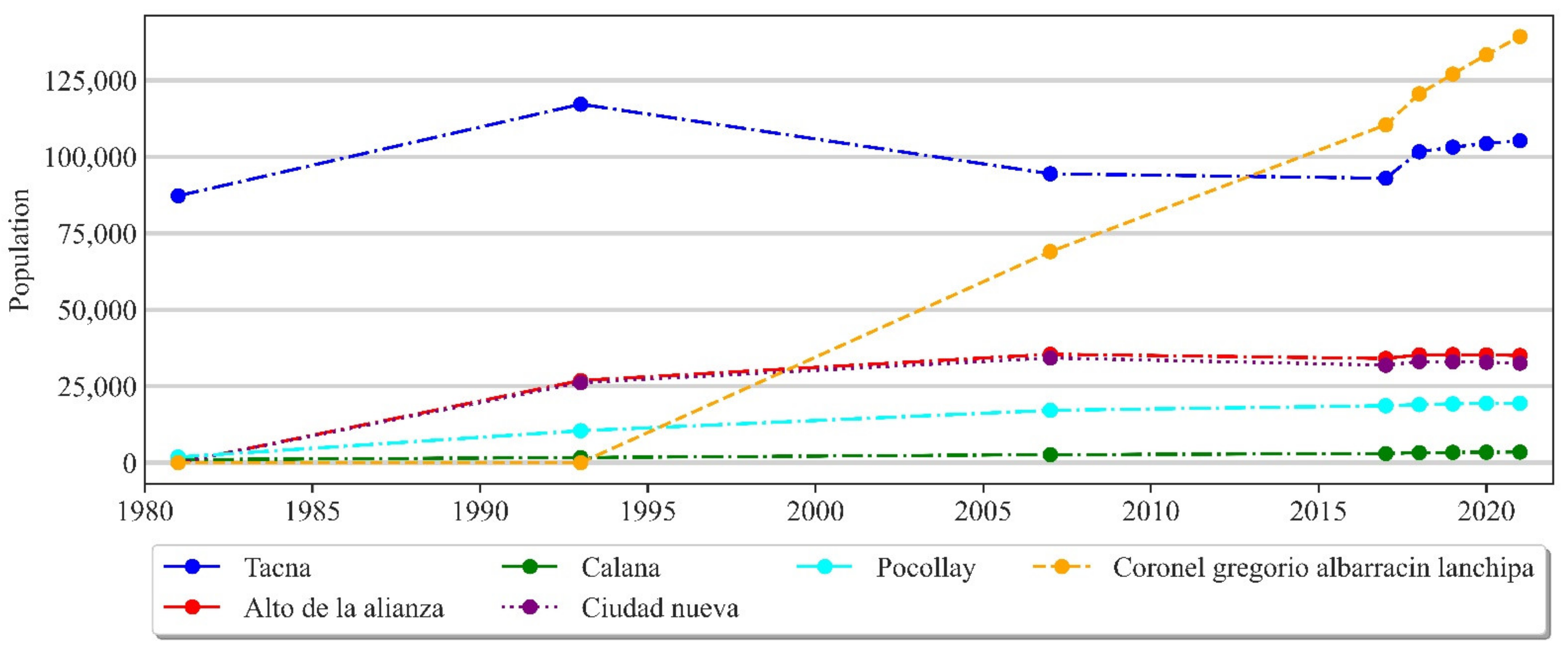
In the city of Tacna, the demographic and concentrated growth of around 91% of the department has generated the accelerated disorderly urban growth and occupation of areas susceptible to natural phenomena. The situation has become a problem for physical security of the inhabitants due to the location of the city, and it is observed that the district of Gregorio Albarracin from 1993 to 2020 had a significant growth (Figure 3 and Figure 4).

3.2. LUCC Analysis Results

The evaluation of the accuracy of LUCC has also been analyzed with the help of the kappa coefficient. For the 1993 LUCC, the kappa value was 0.92, for 2007 the kappa value is 0.89, for 2017 it is 0.96, and for the year 2020 the kappa value is 0.94 (Table 7), which means that both the land use and land cover classification can be interpreted as in almost perfect agreement.
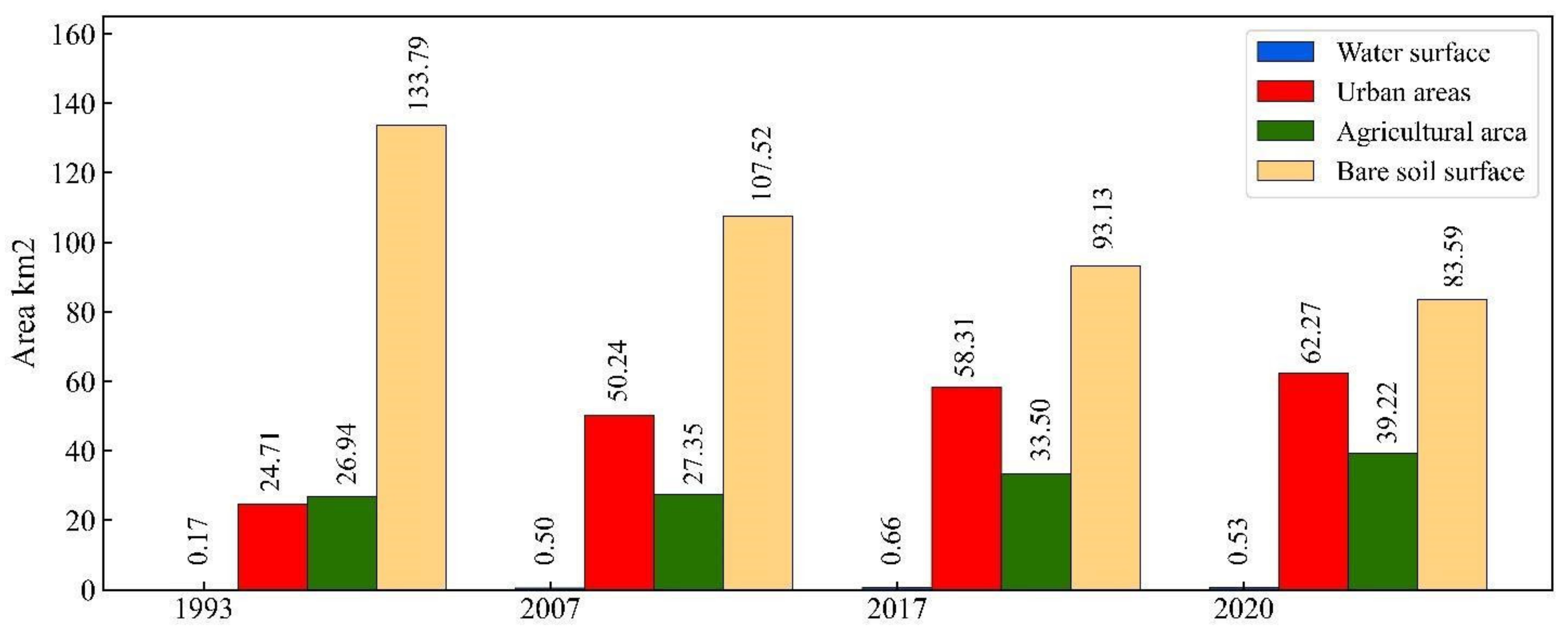
LUCC maps have been classified into four classes, viz., bodies of water, urban area, vegetation, and vacant land and/or bare soil. In 1993, the urban area was observed to be 24.71 km2 (Figure 5), for the year 2020 there was a gain in urban occupation reaching an area of 62.27 km2, and, in parallel, vacant land or bare land was reduced from 133.79 km2 to 83.59 km2. The percentage of area under each LUCC category is represented in Table 8. There was a gain in cultivation area until 2020, growing by 6.6%, and the bodies of water are assumed to be negligible and without impact because Tacna is a city with a high water deficit.

3.3. Verification of Spatial Feature Data

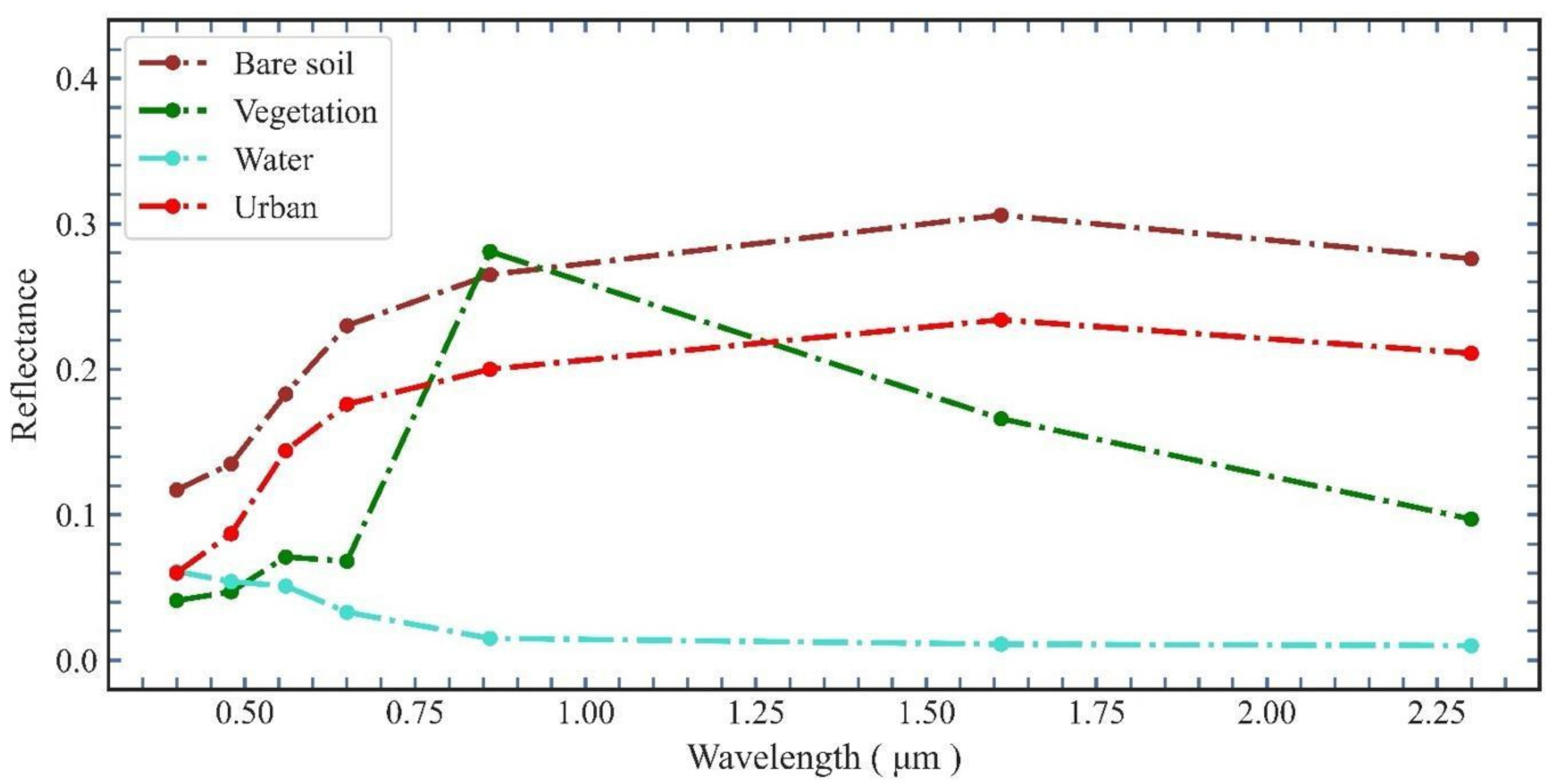
Spectral signature analysis of the urban and other control classes and the spectral profiles for the various classes are presented in Figure 6. Water, bare soil, vegetation, and the urban area show potentially different spectral characteristics along the spectral wavelength. However, the bare ground and urban classes are visually similar by having common shapes along the spectral wavelength, however, there is a slight difference in reflectance values.
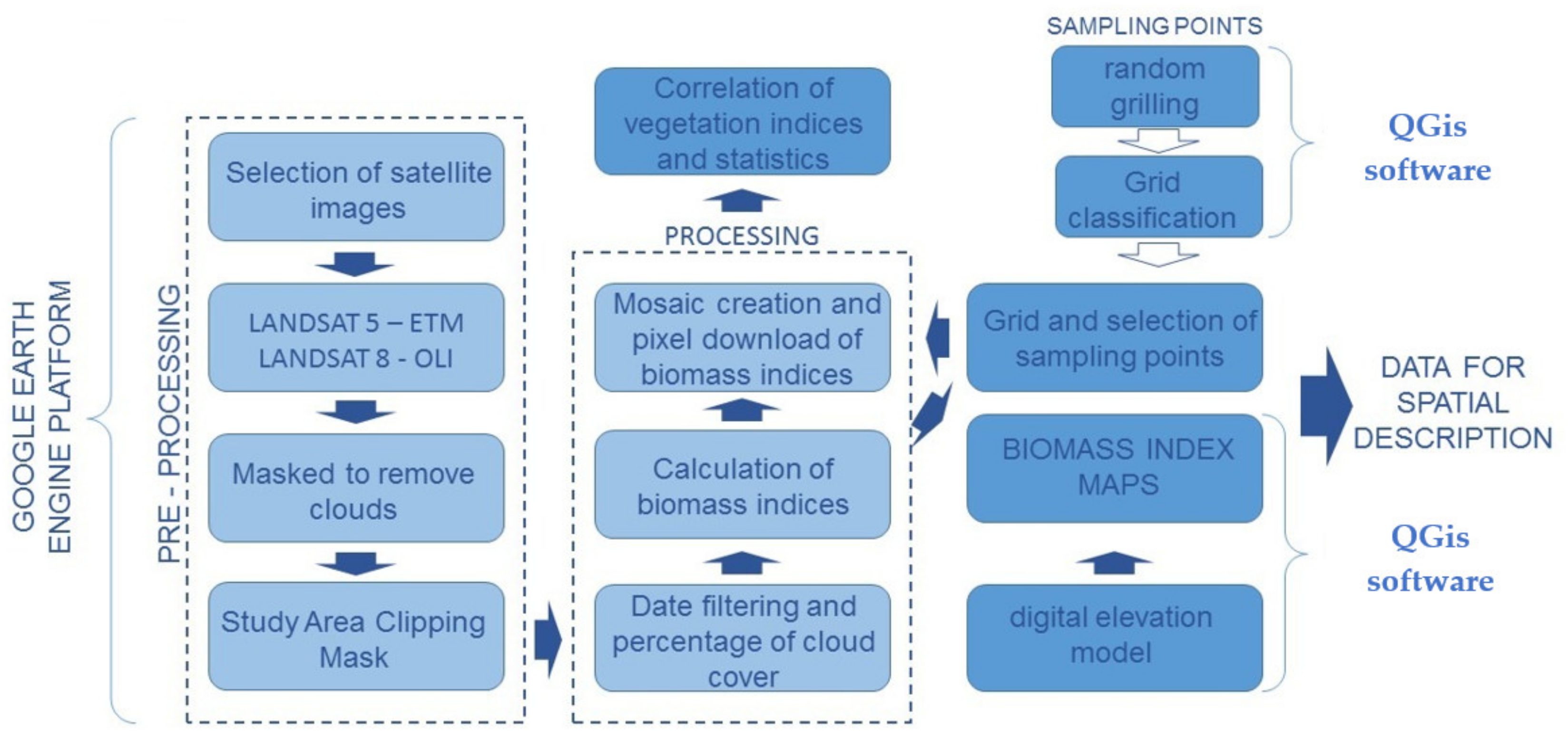
The spectral profile in each pixel represents the unique components of reflectance as a function of the wavelength of the objects (μm). Thus, this allows us to distinguish different objects with similar appearances but different spectral features. Pixel reflectance values in four types were downloaded (urban coverage, bare soil, water, and vegetation) with wavelength values from 0.43 μm to 2.29 μm. This was done using the ID for the Landsat 8 satellite image corrected for surface reflectance (using ID LANDSAT/LC08/C01/T1_SR/LC08_002073_20200312, 12 March 2020: 14 h 41 m 55.51 s) which was available in the Google Earth Engine repository.
For the water profile, the highest reflectance is observed in the visible spectrum (blue band 2) of wavelength equal to 0.45 μm, while decreasing towards the near-infrared region with wavelengths equal to 0.76 μm. The vegetation profile depends on several characteristics (type of species, environmental changes to vegetation cover) and it is interpreted as low in the visible spectrum, even with an increase in green color due to the chlorophyll of the leaves with a value of 0.59 μm, and the reflectance increases in the near infrared due to low energy absorption by plants 0.76 μm. In the mid-infrared region, there is a significant decrease across wavelengths as the plant water absorbs the energy. The urban profile depends on the characteristics of air, water content, granulometric structure, and texture, as buildings are smooth structures, implying that the reflectance increases along the wavelength. In the bare soil, we observe that these non-cultivated soils present a different signature to cultivated soils, and there is an increase along the wavelength since there are no plants that can absorb water.

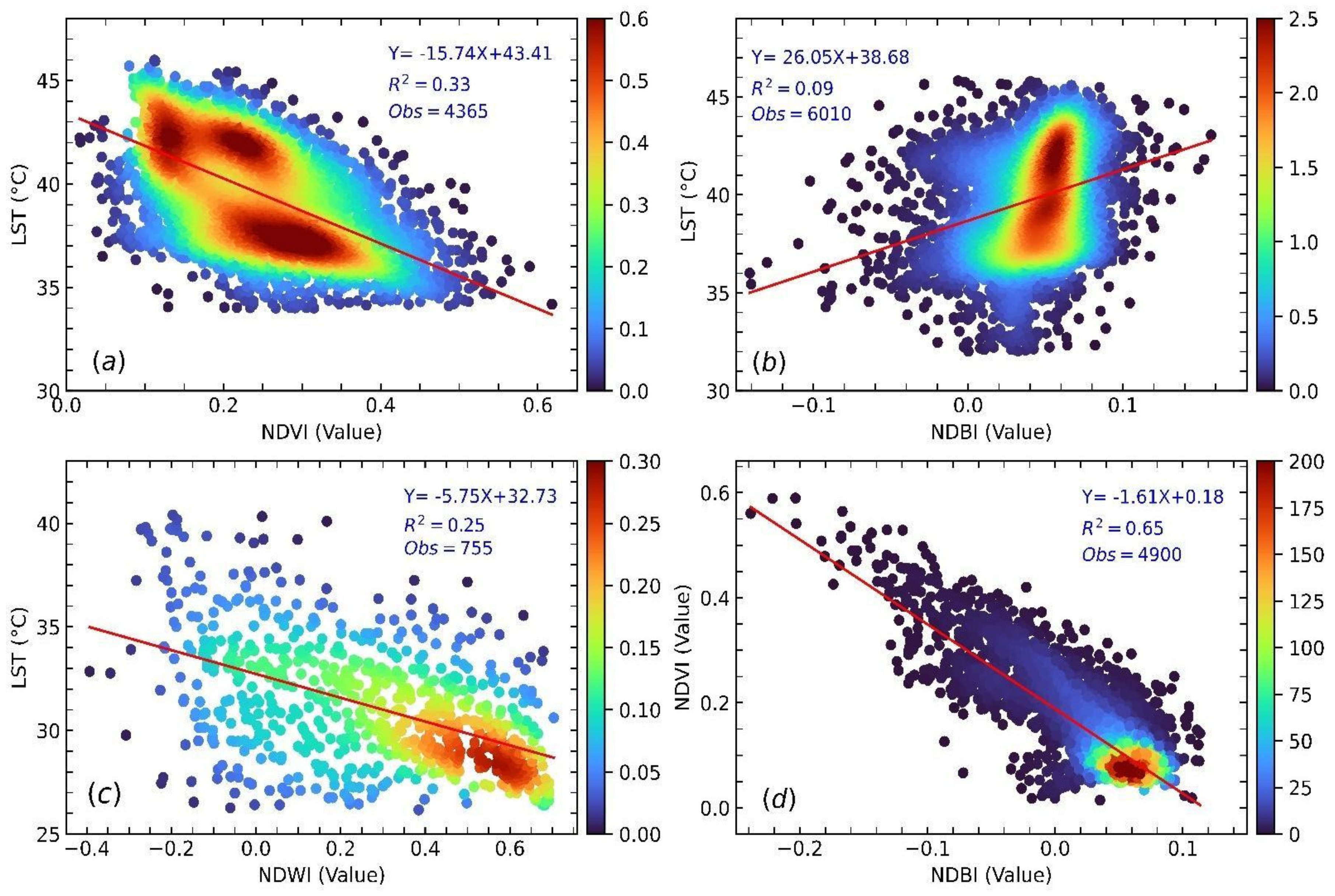
3.4. Correlation Analysis between LST and Spatial Features (NDVI, NDWI, NDBI)

Correlations are established between LST, built-up areas, bodies of water, and vegetation. The maps were obtained for the late summer season in March, due to cloud-free conditions and little atmospheric haze. In this sense, we established a relationship between NDVI and NDBI. Figure 7a shows a negative correlation (coefficient of −0.57) between NDVI and LST for the year 2020, this is attributed to dense vegetation that does not allow the Earth’s surface to receive more radiation. Figure 7b shows a positive correlation between LST and NDBI (coefficient of 0.29), which indicates that there is an increase in surface temperature due to an increase in urbanization and in general infrastructure, and this is a surrogate correlation for population. Figure 7c shows a negative correlation (coefficient of −0.50) between LST and NDWI, mainly due to high values of specific water heat. Figure 7d shows a negative correlation (coefficient of −0.81) between NDVI and NDBI, which means that massive urbanization development brings reduction in vegetation.

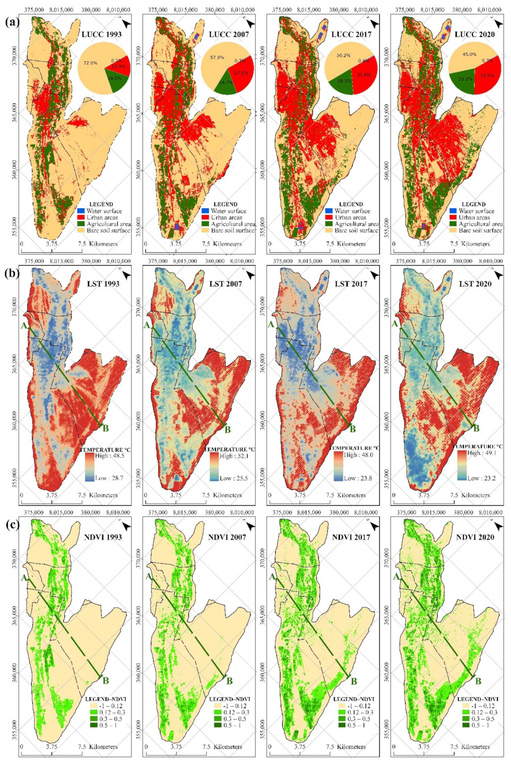
3.5. Correlation Analysis between LST and Population Data

Figure 8 shows the spatial and temporal changes for LUCC (a), LST (b), and NDVI (c). It is clear that urban areas have increased during recent years (from 13.3% in 1993 to 33.5% in 2020). Agricultural areas have increased slightly, and bare soil surface is located along the borders of the domain. More details are presented using the cross section A–B.

3.6. Discussion on the Causes of LST Changes

On a local scale, the climate has changed which is evidenced by the change in the LUCC [25,48,49]. The rate of change in temperature is prominent in the impermeable soil surface [4,50]. To obtain the correlation between LST and LUCC, a cross section (A–B) was generated for each land surface temperature map (1993, 2007, 2017, and 2020) of the late summer season in each year evaluated (Table 9, Figure 8a and 
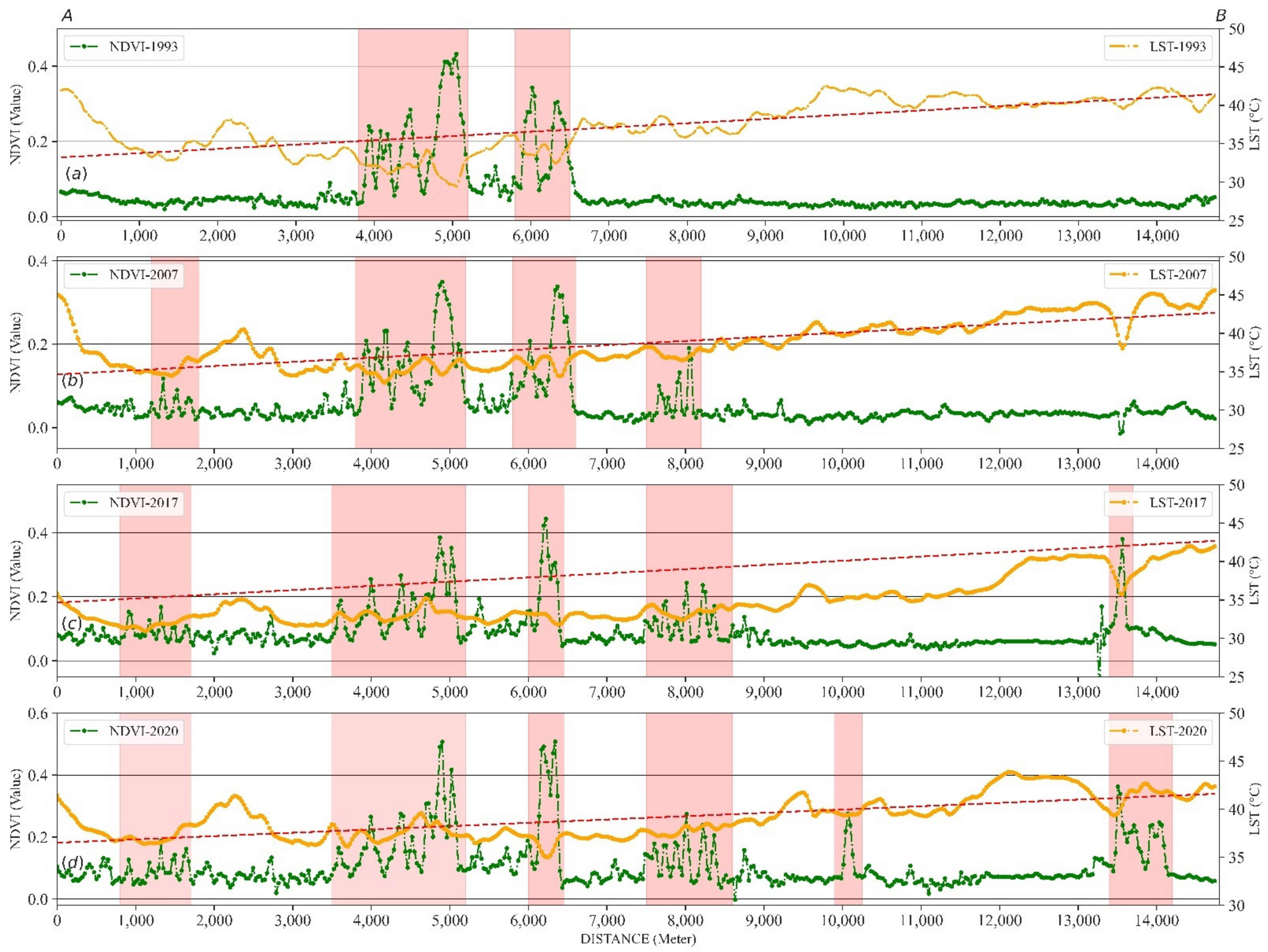
Figure 9). It is observed that on the impermeable surface, mainly in the built area, the temperature varies from 24.2 °C to 44.2 °C, with high temperatures prevailing. Likewise, in areas of vegetation the temperature remains below 24 °C, which is associated with a high rate of potential evapotranspiration.
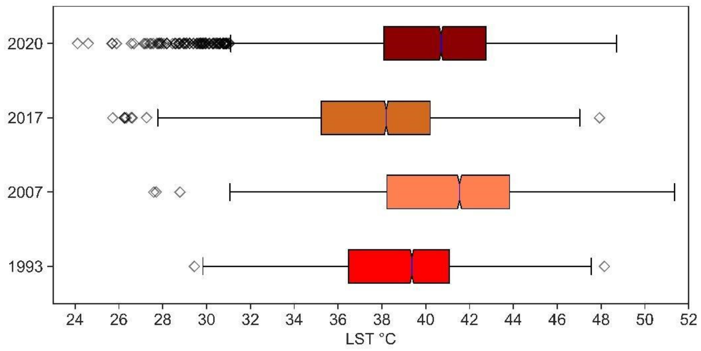
The analysis of the change in temperature of the land surface in time series in relation to land use and land cover units has extracted the change in temperature of the land surface for the years 1993, 2007, 2017, and 2020 for the summer seasons (Figure 8b and Figure 10). For the summer season of 1993, the maximum temperature was 48.1 °C and the minimum was 29.4 °C. However, in 2007 the surface temperature increased in summer, reaching a maximum of 51.3 °C and a minimum of 27.1 °C. Thus, for 2020 there was an increase in its average to 40.3 °C, and it is clear that the maximum temperature during the summer increased up to 0.8 °C, compared to the temperature of the year 2017 (Table 9).
On a micro level, the climate has changed with the change in LUCC units. The rate of temperature change is very prominent on the impermeable surface [4,48]. For correlation between LST and NDVI units, a cross section (A–B) was drawn for each map of Earth’s surface temperature (1993, 2007, 2017, and 2020) of the summer season (Figure 8c and Figure 10). Both figures show that on the impermeable surface, mainly in the vegetation area, the NDVI peaks change inversely proportional to the LST, and the temperature is low due to the high transpiration rate. It varies from 30 °C to 35 °C and high temperatures also prevail in bare soils, where the temperature ranges from 48 °C to 51 °C. High temperatures are consistent with desertic places because it is located at the head of the Atacama Desert, and the urban area is another unit of land cover responsible for the increase in temperature.

3.7. UTFVI Review Results

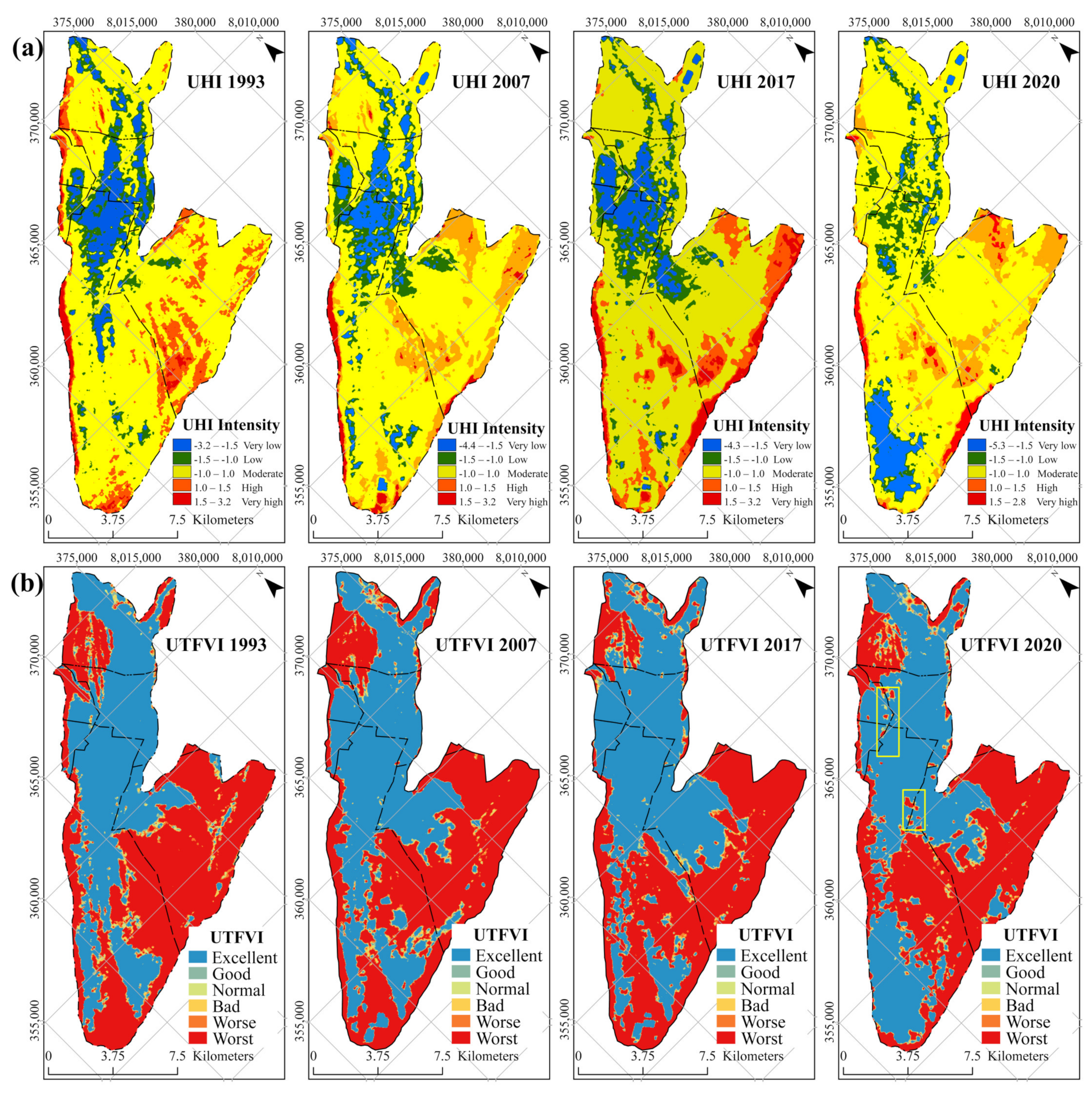
Given that a large part of the analysis area is settled in the morphological units of coastal plains and part of the dissected flank that goes from rugged to hills with steep slopes, for the LUCC temporal analysis of 2020 more than 55% of the land mass of the territory of analysis is developed. Most of the remaining undeveloped land is hills and plains. All of these undeveloped areas have low or no green vegetation cover and excellent ecological assessment index. Due to Tacna’s limited land development, most of the urban development exists in the districts of Gregorio Albarracin, along Tacna’s far northwest, and in scattered settlements in the new territories. Concentrated urban development leads to a degraded eco-environment in these built-up areas with the worst ecological assessment index.
From Figure 11, 2020, it is clear that extreme levels have appeared in the ecological evaluation within the urban area of Tacna: the excellent (<0) and the worst (>0.02) categories. The UTFVI ecological assessment classification map of Tacna can also provide useful information for urban environmental managers to assess eco-environmental quality. The serious phenomenon of urban heat island calls for more reasonable city design and urban development to protect the ecological environment in the future urban plan of Tacna, as is achieved in other similar cities. Based on Figure 11, the middle area of the southwest was bad in 2017, but good in 2020, and this is due to the shrinkage of urban areas.
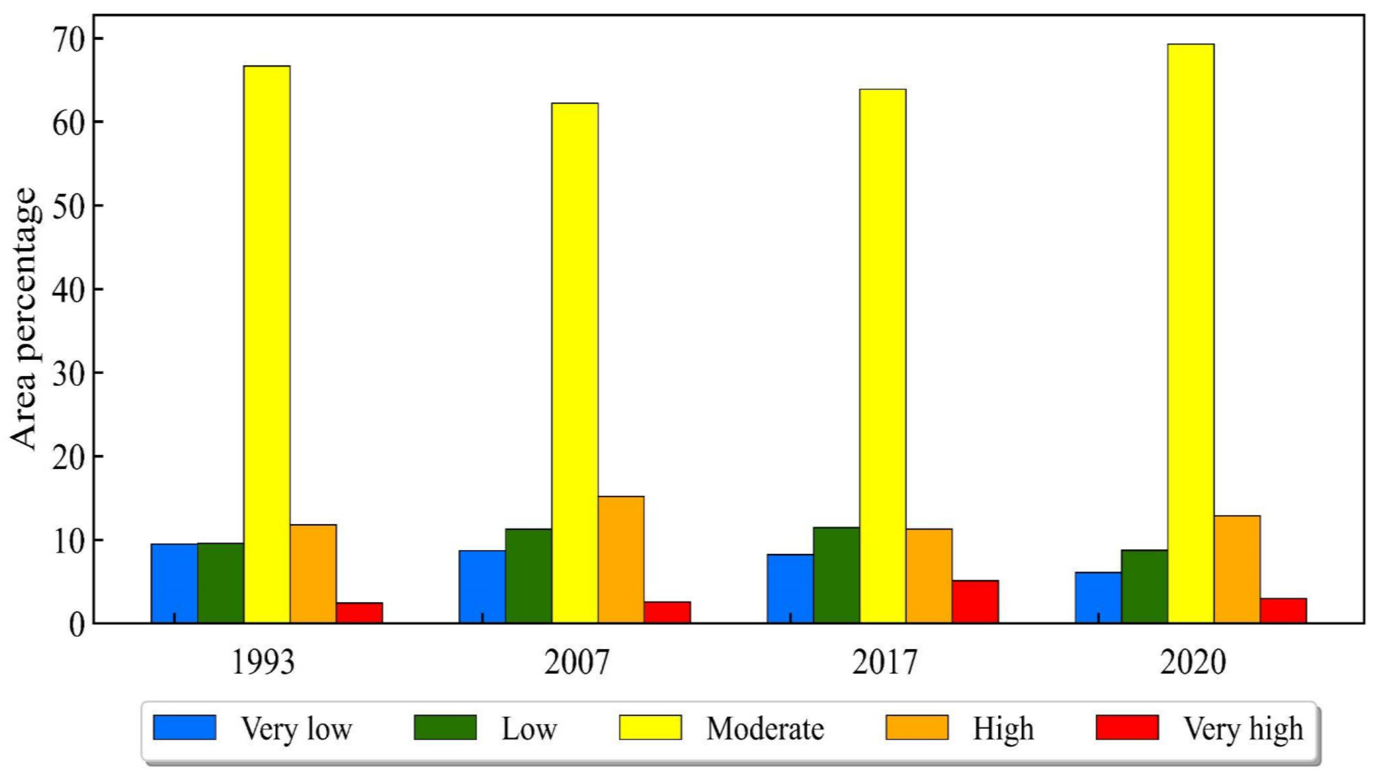
Figure 12 shows temporal changes (from 1993 to 2020) of the UHI intensity in relation to the area (%). The UHI intensity was classified in five different levels: very low, low, moderate, high, and very high. Results show that moderate level UHIs have slightly increased for the last three decades (1993: 66.6%, 2020: 69.3%), very low level UHIs have decreased in area (1993: 9.50%, 2020: 6.09%), high level UHIs have slightly increased (1993: 11.81%, 2020: 12.88%), and very high level UHIs have slightly decreased (1993: 2.44%, 2020: 5.11%).

4. Conclusions

For the conditions free of clouds and atmospheric haze, in the study period, correlations were established between LST, built-up areas, bodies of water, and vegetation, giving good connections between NDVI and NDBI. Likewise, a negative relationship between NDVI and LST is presented for the year 2020, attributable to dense vegetation that does not allow the Earth’s surface to receive radiation.
There is a very high negative correlation (−0.81) between NDBI and NDVI, which means that massive urbanization leads to the reduction in vegetated area. NDBI has a high impact on the LST; a coefficient of connections is recorded as 0.46, as the city of Tacna is one of the most arid regions of Peru, and an increase in the LST is expected with the increase in industrialization and urbanization in the coming years.
The change in the LUCC evidences change in the climate in the city of Tacna since it is observed that in the built areas the temperature varies from 24.2 °C to 44.2 °C, with high temperatures prevailing. In the vegetation areas, the temperature remains below 24 °C, which is associated with a high rate of evapotranspiration.
From the correlation analysis of the recovered LST with NDVI and NDBI, it was found that green land can weaken the urban heat island effect, but built-up land can accelerate the effect. Therefore, we have learned that more attention should be paid to urban greening in future city planning and development.
From the calculation of the ecological evaluation index using the UTFVI classification, it is seen that Tacna has the strongest urban heat island phenomenon and the worst ecological environment, strongly calling for more reasonable urban design and urban development in the future.
This study was performed using freely available remote sensing data for estimating the UHI in the Tacna area. In the present study, the UHI estimation does not consider additional climatic and landscape parameters and it was focused mostly on the summer period, thus a deeper study (including monitoring efforts) should be developed, especially for arid cities.

Author Contributions

Conceptualization, E.P.-V., J.E.-M. and J.A.; methodology, E.P.-V., K.A.-C. and G.H.; software, G.H. and E.C.-V.; validation, J.E.-M., E.P.-V., K.A.-C., G.H., J.A. and E.C.-V.; formal analysis, J.E.-M., G.H. and J.A.; investigation, G.H. and E.C.-V.; writing—original draft preparation, J.E.-M. and E.P.-V.; writing—review and editing, J.E.-M., E.P.-V., K.A.-C., G.H., J.A. and E.C.-V.; supervision, E.P.-V.; project administration, E.P.-V. All authors have read and agreed to the published version of the manuscript.

Funding

This research and the APC was funded by Jorge Basadre Grohmann National University, proyect approved R.C.U. No. 16775-2020-UN/JBG.

Institutional Review Board Statement

Not applicable.

Informed Consent Statement

Not applicable.

Data Availability Statement

Not applicable.

Acknowledgments

Research project financed with canon, surcharge, and mining royalty funds Study of risk and alternatives of protection of the population in the area of influence of the creek of the Devil, Tacna, Peru. Jorge Basadre Grohmann National University.

Conflicts of Interest

The authors declare no conflict of interest.

References

  1. Kong, J.; Zhao, Y.; Carmeliet, J.; Lei, C. Urban Heat Island and Its Interaction with Heatwaves: A Review of Studies on Mesoscale. Sustainability 2021, 13, 10923. [Google Scholar] [CrossRef]
  2. Oke, T.R.; Mills, G.; Christen, A.; Voogt, J.A. Urban Climates; Cambridge University Press: Cambridge, UK, 2017. [Google Scholar]
  3. Dilawar, A.; Chen, B.; Trisurat, Y.; Tuankrua, V.; Arshad, A.; Hussain, Y.; Measho, S.; Guo, L.; Kayiranga, A.; Zhang, H.; et al. Spatiotemporal Shifts in Thermal Climate in Responses to Urban Cover Changes: A-Case Analysis of Major Cities in Punjab, Pakistan. Geomat. Nat. Hazards Risk 2021, 12, 763–793. [Google Scholar] [CrossRef]
  4. Ranagalage, M.; Ratnayake, S.S.; Dissanayake, D.; Kumar, L.; Wickremasinghe, H.; Vidanagama, J.; Cho, H.; Udagedara, S.; Jha, K.K.; Simwanda, M.; et al. Spatiotemporal Variation of Urban Heat Islands for Implementing Nature-Based Solutions: A Case Study of Kurunegala, Sri Lanka. ISPRS Int. J. Geo-Inf. 2020, 9, 461. [Google Scholar] [CrossRef]
  5. Huerto-Cardenas, H.E.; Aste, N.; Del Pero, C.; Della Torre, S.; Leonforte, F. Effects of Climate Change on the Future of Heritage Buildings: Case Study and Applied Methodology. Climate 2021, 9, 132. [Google Scholar] [CrossRef]
  6. Tian, Y.; Wang, R.; Liu, L.; Ren, Y. A Spatial Effect Study on Financial Agglomeration Promoting the Green Development of Urban Agglomerations. Sustain. Cities Soc. 2021, 70, 102900. [Google Scholar] [CrossRef]
  7. Sabrin, S.; Karimi, M.; Nazari, R. Developing Vulnerability Index to Quantify Urban Heat Islands Effects Coupled with Air Pollution: A Case Study of Camden, NJ. ISPRS Int. J. Geo-Inf. 2020, 9, 349. [Google Scholar] [CrossRef]
  8. Simperler, L.; Ertl, T.; Matzinger, A. Spatial Compatibility of Implementing Nature-Based Solutions for Reducing Urban Heat Islands and Stormwater Pollution. Sustainability 2020, 12, 5967. [Google Scholar] [CrossRef]
  9. Ozawa-Meida, L.; Ortiz-Moya, F.; Painter, B.; Hengesbaugh, M.; Nakano, R.; Yoshida, T.; Zusman, E.; Bhattacharyya, S. Integrating the Sustainable Development Goals (SDGs) into Urban Climate Plans in the UK and Japan: A Text Analysis. Climate 2021, 9, 100. [Google Scholar] [CrossRef]
  10. Helletsgruber, C.; Gillner, S.; Gulyás, Á.; Junker, R.R.; Tanács, E.; Hof, A. Identifying Tree Traits for Cooling Urban Heat Islands—A Cross-City Empirical Analysis. Forests 2020, 11, 1064. [Google Scholar] [CrossRef]
  11. Das, N.; Mondal, P.; Sutradhar, S.; Ghosh, R. Assessment of Variation of Land Use/Land Cover and Its Impact on Land Surface Temperature of Asansol Subdivision. Egypt. J. Remote Sens. Space Sci. 2021, 24, 131–149. [Google Scholar] [CrossRef]
  12. Gao, Z.; Hou, Y.; Zaitchik, B.F.; Chen, Y.; Chen, W. A Two-Step Integrated MLP-GTWR Method to Estimate 1 Km Land Surface Temperature with Complete Spatial Coverage in Humid, Cloudy Regions. Remote Sens. 2021, 13, 971. [Google Scholar] [CrossRef]
  13. Tang, K.; Zhu, H.; Ni, P. Spatial Downscaling of Land Surface Temperature over Heterogeneous Regions Using Random Forest Regression Considering Spatial Features. Remote Sens. 2021, 13, 3645. [Google Scholar] [CrossRef]
  14. Parastatidis, D.; Mitraka, Z.; Chrysoulakis, N.; Abrams, M. Online Global Land Surface Temperature Estimation from Landsat. Remote Sens. 2017, 9, 1208. [Google Scholar] [CrossRef] [Green Version]
  15. Quattrochi, D.A.; Luvall, J.C. Thermal Infrared Remote Sensing for Analysis of Landscape Ecological Processes: Methods and Applications. Landsc. Ecol. 1999, 14, 577–598. [Google Scholar] [CrossRef]
  16. Wu, X.; Wang, G.; Yao, R.; Wang, L.; Yu, D.; Gui, X. Investigating Surface Urban Heat Islands in South America Based on MODIS Data from 2003–2016. Remote Sens. 2019, 11, 1212. [Google Scholar] [CrossRef] [Green Version]
  17. Barbosa, G.S.; Drach, P.R.C.; Corbella, O.D. Intraurban Temperature Variations: Urban Morphologies of the Densification Process of Copacabana Neighborhood, Brazil. Climate 2019, 7, 65. [Google Scholar] [CrossRef] [Green Version]
  18. Palme, M.; Lobato, A.; Carrasco, C. Quantitative Analysis of Factors Contributing to Urban Heat Island Effect in Cities of Latin-American Pacific Coast. Procedia Eng. 2016, 169, 199–206. [Google Scholar] [CrossRef]
  19. Villegas-Lanza, J.C.; Chlieh, M.; Cavalié, O.; Tavera, H.; Baby, P.; Chire-Chira, J.; Nocquet, J.-M. Active Tectonics of Peru: Heterogeneous Interseismic Coupling along the Nazca Megathrust, Rigid Motion of the Peruvian Sliver, and Subandean Shortening Accommodation. J. Geophys. Res. Solid Earth 2016, 121, 7371–7394. [Google Scholar] [CrossRef]
  20. Preston, S.H. Urban Growth in Developing Countries: A Demographic Reappraisal. Popul. Dev. Rev. 1979, 5, 195. [Google Scholar] [CrossRef]
  21. Hegazy, I.R.; Kaloop, M.R. Monitoring Urban Growth and Land Use Change Detection with GIS and Remote Sensing Techniques in Daqahlia Governorate Egypt. Int. J. Sustain. Built Environ. 2015, 4, 117–124. [Google Scholar] [CrossRef] [Green Version]
  22. Green, A.A.; Berman, M.; Switzer, P.; Craig, M.D. A Transformation for Ordering Multispectral Data in Terms of Image Quality with Implications for Noise Removal. IEEE Trans. Geosci. Remote Sens. 1988, 26, 65–74. [Google Scholar] [CrossRef] [Green Version]
  23. Weng, Q.; Lu, D.; Schubring, J. Estimation of Land Surface Temperature–Vegetation Abundance Relationship for Urban Heat Island Studies. Remote Sens. Environ. 2004, 89, 467–483. [Google Scholar] [CrossRef]
  24. Voogt, J.; Oke, T. Thermal Remote Sensing of Urban Climates. Remote Sens. Environ. 2003, 86, 370–384. [Google Scholar] [CrossRef]
  25. Pino-Vargas, E.; Chávarri-Velarde, E.; Ingol-Blanco, E.; Mejía, F.; Cruz, A.; Vera, A. Impacts of Climate Change and Variability on Precipitation and Maximum Flows in Devil’s Creek, Tacna, Peru. Hydrology 2022, 9, 10. [Google Scholar] [CrossRef]
  26. Pino, E.; Ramos, L.; Avalos, O.; Tacora, P.; Chávarri, E.; Angulo, O.; Ascensios, D.; Mejía, J. Factores Que Inciden En El Agotamiento y La Contaminación Por Intrusión Marina En El Acuífero Costero de La Yarada, Tacna, Perú. Tecnol. Cienc. Agua 2019, 10, 177–213. [Google Scholar] [CrossRef]
  27. Pino, E.; Chávarri, E.; Ramos, L. Governability and Governance Crisis Its Implications in the Inadequate Use of Groundwater, Case Coastal Aquifer of La Yarada, Tacna, Perú. Idesia 2018, 36, 77–85. [Google Scholar]
  28. Pino, E. El Acuífero Costero La Yarada, Después de 100 Años de Explotación Como Sustento de Una Agricultura En Zonas Áridas: Una Revisión Histórica. Idesia 2019, 37, 39–45. [Google Scholar] [CrossRef] [Green Version]
  29. Pino, E. Conflicts over the Use of Water in an Arid Region: Case of Tacna, Peru. Diálogo Andino 2021, 65, 406–415. [Google Scholar]
  30. Pino, E.; Chávarri, E. Evidencias de Cambio Climático En La Región Hiperárida de La Costa Sur de Perú, Cabecera Del Desierto de Atacama. Tecnol. Cienc. Agua 2022, 13, 333–376. [Google Scholar] [CrossRef]
  31. Narvaez-Montoya, C.; Torres-Martínez, J.A.; Pino-Vargas, E.; Cabrera-Olivera, F.; Loge, F.J.; Mahlknecht, J. Predicting Adverse Scenarios for a Transboundary Coastal Aquifer System in the Atacama Desert (Peru/Chile). Sci. Total Environ. 2022, 806, 150386. [Google Scholar] [CrossRef]
  32. Pino, E.; Montalván, I.; Vera, A.; Ramos, L. La Conductancia Estomática y Su Relación Con La Temperatura Foliar y Humedad Del Suelo En El Cultivo Del Olivo (Olea europaea, L.), En Periodo de Maduración de Frutos, En Zonas Áridas.La Yarada, Tacna, Perú. Idesia 2019, 37, 55–64. [Google Scholar] [CrossRef]
  33. Stein, B.A.; Staudt, A.; Cross, M.S.; Dubois, N.S.; Enquist, C.; Griffis, R.; Hansen, L.J.; Hellmann, J.J.; Lawler, J.J.; Nelson, E.J.; et al. Preparing for and Managing Change: Climate Adaptation for Biodiversity and Ecosystems. Front. Ecol. Environ. 2013, 11, 502–510. [Google Scholar] [CrossRef]
  34. Abrook, A.M.; Matthews, I.P.; Milner, A.M.; Candy, I.; Palmer, A.P.; Timms, R.G.O. Environmental Variability in Response to Abrupt Climatic Change during the Last Glacial–Interglacial Transition (16–8 Cal Ka BP): Evidence from Mainland, Orkney. Scott. J. Geol. 2020, 56, 30–46. [Google Scholar] [CrossRef]
  35. Alvino, F.C.G.; Aleman, C.C.; Filgueiras, R.; Althoff, D.; da Cunha, F.F. Vegetation Indices for Irrigated Corn Monitoring. Eng. Agrícola 2020, 40, 322–333. [Google Scholar] [CrossRef]
  36. Jimenez-Munoz, J.C.; Sobrino, J.A.; Skokovic, D.; Mattar, C.; Cristobal, J. Land Surface Temperature Retrieval Methods From Landsat-8 Thermal Infrared Sensor Data. IEEE Geosci. Remote Sens. Lett. 2014, 11, 1840–1843. [Google Scholar] [CrossRef]
  37. Jimenez-Munoz, J.C.; Cristobal, J.; Sobrino, J.A.; Soria, G.; Ninyerola, M.; Pons, X.; Pons, X. Revision of the Single-Channel Algorithm for Land Surface Temperature Retrieval From Landsat Thermal-Infrared Data. IEEE Trans. Geosci. Remote Sens. 2009, 47, 339–349. [Google Scholar] [CrossRef]
  38. Sobrino, J.A.; Jiménez-Muñoz, J.C.; Paolini, L. Land Surface Temperature Retrieval from LANDSAT TM 5. Remote Sens. Environ. 2004, 90, 434–440. [Google Scholar] [CrossRef]
  39. Alatorre, L.C.; Díaz, R.E.; Miramontes, S.; Bravo, L.C.; Sánchez, E. Spatial and Temporal Evolution of the Static Water Level of the Cuauhtemoc Aquifer during the Years 1973, 1991 and 2000: A Geographical Approach. J. Geogr. Inf. Syst. 2014, 06, 572–584. [Google Scholar] [CrossRef] [Green Version]
  40. Aboutalebi, M.; Torres-Rua, A.F.; McKee, M.; Kustas, W.; Nieto, H.; Coopmans, C. Behavior of Vegetation/Soil Indices in Shaded and Sunlit Pixels and Evaluation of Different Shadow Compensation Methods Using UAV High-Resolution Imagery over Vineyards. In Proceedings of the SPIE 10664, Autonomous Air and Ground Sensing Systems for Agricultural Optimization and Phenotyping III, Orlando, FL, USA, 15–19 April 2018; p. 6. [Google Scholar]
  41. Ermida, S.L.; Soares, P.; Mantas, V.; Göttsche, F.-M.; Trigo, I.F. Google Earth Engine Open-Source Code for Land Surface Temperature Estimation from the Landsat Series. Remote Sens. 2020, 12, 1471. [Google Scholar] [CrossRef]
  42. Ahmed, S. Assessment of Urban Heat Islands and Impact of Climate Change on Socioeconomic over Suez Governorate Using Remote Sensing and GIS Techniques. Egypt. J. Remote Sens. Space Sci. 2018, 21, 15–25. [Google Scholar] [CrossRef]
  43. Liu, L.; Zhang, Y. Urban Heat Island Analysis Using the Landsat TM Data and ASTER Data: A Case Study in Hong Kong. Remote Sens. 2011, 3, 1535–1552. [Google Scholar] [CrossRef] [Green Version]
  44. Svoboda, J.; Štych, P.; Laštovička, J.; Paluba, D.; Kobliuk, N. Random Forest Classification of Land Use, Land-Use Change and Forestry (LULUCF) Using Sentinel-2 Data—A Case Study of Czechia. Remote Sens. 2022, 14, 1189. [Google Scholar] [CrossRef]
  45. Jiao, W.; Hao, X.; Qin, C. The Image Classification Method with CNN-XGBoost Model Based on Adaptive Particle Swarm Optimization. Information 2021, 12, 156. [Google Scholar] [CrossRef]
  46. Li, C.; Ma, Z.; Wang, L.; Yu, W.; Tan, D.; Gao, B.; Feng, Q.; Guo, H.; Zhao, Y. Improving the Accuracy of Land Cover Mapping by Distributing Training Samples. Remote Sens. 2021, 13, 4594. [Google Scholar] [CrossRef]
  47. Roldán-Nofuentes, J.A.; Regad, S.B. Estimation of the Average Kappa Coefficient of a Binary Diagnostic Test in the Presence of Partial Verification. Mathematics 2021, 9, 1694. [Google Scholar] [CrossRef]
  48. Vera, A.; Pino-Vargas, E.; Verma, M.P.; Chucuya, S.; Chávarri, E.; Canales, M.; Torres-Martínez, J.A.; Mora, A.; Mahlknecht, J. Hydrodynamics, Hydrochemistry, and Stable Isotope Geochemistry to Assess Temporal Behavior of Seawater Intrusion in the La Yarada Aquifer in the Vicinity of Atacama Desert, Tacna, Peru. Water 2021, 13, 3161. [Google Scholar] [CrossRef]
  49. Pino, E.; Ramos, L.; Mejía, J.; Chávarri, E.; Ascensios, D. Medidas de Mitigación Para El Acuífero Costero La Yarada, Un Sistema Sobreexplotado En Zonas Áridas. Idesia 2020, 38, 21–31. [Google Scholar] [CrossRef]
  50. Ranagalage, M.; Wang, R.; Gunarathna, M.H.J.P.; Dissanayake, D.M.S.L.B.; Murayama, Y.; Simwanda, M. Spatial Forecasting of the Landscape in Rapidly Urbanizing Hill Stations of South Asia: A Case Study of Nuwara Eliya, Sri Lanka (1996–2037). Remote Sens. 2019, 11, 1743. [Google Scholar] [CrossRef] [Green Version]
Figure 1. Location map of the study area, Tacna city, Peru. (a) Location of Peru in South America, (b) location of Tacna in Peru, and (c) urbanized area in Tacna.
Climate 10 00087 g001
Figure 2. Work diagram with the Landsat 5 and 8 satellite images on the Google Earth Engine platform, to obtain the temporal maps (1993–2020), and the characterization of the spatial variability of the heat indices.
Climate 10 00087 g002
Figure 3. Population growth by district, according to the study area (1981–2021).
Climate 10 00087 g003
Figure 4. Multitemporal growth by districts from 1981 to 2020.
Climate 10 00087 g004
Figure 5. Temporal variation (from 1993 to 2020) of the water surface, urban areas, agricultural area, and bare soil surface.
Climate 10 00087 g005
Figure 6. Spectral profile of urban area and control classes.
Climate 10 00087 g006
Figure 7. (a) Relationship between LST and NDVI, (b) LST and NDBI, (c) LST and NDWI (2020), (d) NDVI and NDBI.
Climate 10 00087 g007
Figure 8. Temporal variation period 1993 to 2020 for maximum summer values. (a) LUCC, (b) LST, and (c) NDVI.
Climate 10 00087 g008
Figure 9. Representation of the dispersion and symmetry of LST, for the years 1993, 2007, 2017, and 2020.
Climate 10 00087 g009
Figure 10. Cross section temporal profiles A–B of LST and NDVI for the years (a) 1993, (b) 2007, (c) 2017, and (d) 2020, between 1993 and 2020, we observed a sustained increase in NDVI and, in turn, a growth in LST.
Climate 10 00087 g010
Figure 11. Representation for 1993–2020 of (a) UHI, (b) UTFVI classification map of ecological evaluation in Tacna.
Climate 10 00087 g011
Figure 12. Temporal changes of UHI intensity in relation to area.
Climate 10 00087 g012
Table 1. Landsat 5 and 8 thermal bands: wavelengths, spatial resolution, and time period.
Thermal Band(s)Wavelength (μm)Spatial Resolution (m)Time Period
Landsat 5Band 610.40–12.50120 (30) 1February 1993–February 2007
Landsat 8Band 1010.60–11.19100 (30) 1March 2015–March 2020
Banda 1111.50–12.51
1 Thermal band data are acquired at a lower resolution and resampled with cubic convolution at a higher spatial resolution before distribution as products by USGS.
Table 2. Downloaded LST scenes, Landsat, Remote Sensing Lab (http://rslab.gr/downloadsLandsatLST.html) (accessed on 14 February 1993).
DataYearProduct IdentifierSensing Time
(hh:mm:ss)
PatchRow
Landsat 51993LT05_002072_1993021414:03:36.0400272
1993LT05_002073_1993021414:03:59.8330273
Landsat 52007LT05_002072_2007020514:36:37.0540272
2007LT05_002073_2007020514:37:00.8840273
Landsat 82017LC08_002072_2017040514:41:11.3270272
2017LC08_002073_2017040514:41:35.2570273
Landsat 82020LC08_002072_2020031214:41:31.5820272
2020LC08_002073_2020031214:41:55.5110273
Table 3. The threshold of ecological evaluation index.
Urban Thermal Field Variance IndexUrban Heat Island PhenomenonEcological Evaluation Index
<0NoneExcellent
0.000–0.005WeakGood
0.005–0.010MiddleNormal
0.015–0.015StrongBad
0.015–0.020StrongerWorse
>0.020StrongestWorst
Table 4. Vegetation index equations.
IndexDescriptionEquationReference
NDVINormalized Difference Vegetation Index NDVI = NIR RED NIR + RED [39,40]
NDWINormalized Difference Water Index NDWI = NIR SWIR NIR + SWIR [11]
NDBINormalized Difference Built-up Index NDBI = MIR NIR MIR + NIR [11]
Table 5. Land use and land cover types in the study area.
LUCC ClassesDescription
Water surfaceTank, pond, river, etc.
Urban areasUrban and rural built-up, roads, buildings, and concrete structures
Agricultural areaUrban plantation, agricultural plantation, bushes, etc.
Bare soil surfaceExposed rock, waste lands, bare soil, impervious surface, etc.
Table 6. Observations of the agreement for the kappa coefficient.
Kappa-Hat ValueNature of the Agreement
0.8 ≤ k ≥ 1Almost perfect agreement
0.61 ≤ k ≥ 0.8Substantial agreement
0.41 ≤ k ≥ 0.6Moderate agreement
0.21 ≤ k ≥ 0.4Fair deal
0.0 ≤ k ≥ 0.2Slight agreement
k < 0.0Bad deal
Table 7. 1993–2020 land use and land cover accuracy assessment.
YearLand Cover GroundWater SurfaceUrban AreasAgricultural AreaBare SoilTotalUser AccuracyKappa Coefficient (k)
1993Water surface500051000.92
Urban areas012031580
Agricultural area0038038100
Bare soil020384095
Total514384198
Producer accuracy10085.710092.6378.3
Overall accuracy0.95
2007Water surface26000261000.89
Urban areas035023795
Agricultural area0050050100
Bare soil090263574
Total26445028148
Producer accuracy1008010093372.4
Overall accuracy0.92
2017Water surface23000231000.96
Urban areas025032889
Agricultural area0041041100
Bare soil0002323100
Total23254126115
Producer accuracy10010010088388.5
Overall accuracy0.97
2020Water surface31000311000.94
Urban areas023022592
Agricultural area0028028100
Bare soil011151788
Total31242917101
Producer accuracy100969788380.6
Overall accuracy0.96
Table 8. LUCC area percentage for each category.
LUCC CategoryPercentage (%)
1993200720172020
Water surface0.10.30.40.3
Urban areas13.327.031.333.4
Agricultural area14.514.718.021.1
Bare soil surface71.957.750.044.9
Table 9. LST statistics for the study period.
Statistical
LST °C
1993200720172020
Count8603860386038603
Mean38.741.037.840.3
Std3.033.43.13.1
Minimum29.427.525.724.1
25%36.438.235.238.0
50%39.341.538.240.7
75%41.043.840.242.7
Maximum48.151.347.948.7
Publisher’s Note: MDPI stays neutral with regard to jurisdictional claims in published maps and institutional affiliations.

